classification - linear svmsvm { discussions nonlinear separable cs479/579: data mining slide-13...
TRANSCRIPT

Linear Support Vector Machine
ClassificationLinear SVM
Huiping Cao
Huiping Cao, Slide 1/26

Linear Support Vector Machine
Support Vector Machines
Find a linear hyperplane (decision boundary) that will separate thedata.
CS479/579: Data Mining Slide-2
Support Vector Machines
Find a linear hyperplane (decision boundary) that will separate the data Huiping Cao, Slide 2/26

Linear Support Vector Machine
Support Vector Machines
One possible solution.
CS479/579: Data Mining Slide-3
Support Vector Machines
One Possible Solution
B1
Huiping Cao, Slide 3/26

Linear Support Vector Machine
Support Vector Machines
Another possible solution.
CS479/579: Data Mining Slide-4
Support Vector Machines
Another possible solution
B2
Huiping Cao, Slide 4/26

Linear Support Vector Machine
Support Vector Machines
Other possible solutions.
CS479/579: Data Mining Slide-5
Support Vector Machines
Other possible solutions
B2
Huiping Cao, Slide 5/26

Linear Support Vector Machine
Support Vector Machines
Which one is better? B1 or B2?How do you define better? The bigger the margin, the better.
CS479/579: Data Mining Slide-6
Support Vector Machines
Which one is better? B1 or B2? How do you define better?
B1
B2
Huiping Cao, Slide 6/26

Linear Support Vector Machine
Support Vector Machines
Find hyperplane that maximizes the margin; so B1 is better thanB2
CS479/579: Data Mining Slide-7
Support Vector Machines
Find hyperplane maximizes the margin => B1 is better than B2
B1
B2
b11
b12
b21b22
margin
Huiping Cao, Slide 7/26

Linear Support Vector Machine
Support Vector Machines
CS479/579: Data Mining Slide-8
Support Vector Machines
0=+• bxw
B1
b11
b12
1−=+• bxw
1+=+• bxw
⎩⎨⎧
−≤+•−
≥+•=
1bxw if11bxw if1
)(
xf Margin = 2|| !w ||
B1 : wᵀx + b = 0
b11 : wᵀx + b = 1
b12 : wᵀx + b = −1
Huiping Cao, Slide 8/26

Linear Support Vector Machine
Support Vector Machines
0=+• bxw B1
b11
b12
!w• !x + b = +1
!w• !x + b = !1!w
X2 X1
d
The margin of the decision boundaries:
wᵀ(x1 − x2) = 2wᵀ(x1 − x2) = ‖w‖ × ‖(x1 − x2)‖ × cos(θ) , where ‖ · ‖ is thenorm of a vector.‖w‖ × ‖(x1 − x2)‖ × cos(θ) = ‖w‖ × d , where d is the lengthof vector (x1 − x2) in the direction of vector wThus, ‖w‖ × d = 2Margin: d = 2
‖w‖
Huiping Cao, Slide 9/26

Linear Support Vector Machine
Learn a linear SVM Model
The training phase of SVM is to estimate the parameters wand b.
The parameters must follow two conditions:
yi =
{1, if wᵀxi + b ≥ 1
−1, if wᵀxi + b ≤ −1
Huiping Cao, Slide 10/26
Linear Support Vector Machine
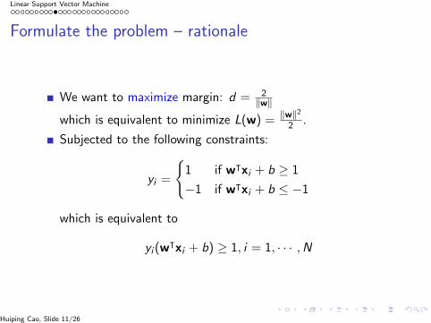
Formulate the problem – rationale
We want to maximize margin: d = 2‖w‖
which is equivalent to minimize L(w) = ‖w‖2
2 .
Subjected to the following constraints:
yi =
{1 if wᵀxi + b ≥ 1
−1 if wᵀxi + b ≤ −1
which is equivalent to
yi (wᵀxi + b) ≥ 1, i = 1, · · · ,N
Huiping Cao, Slide 11/26

Linear Support Vector Machine
Formulate the problem
Formalized to the following constrained optimization problem.Objective function:
Minimize‖w‖2
2
subject toyi (w
ᵀxi + b) ≥ 1, i = 1, · · · ,NConvex optimization problem:
Objective function is quadraticConstraints are linearCan be solved using the standard Lagrange multipliermethod.
Huiping Cao, Slide 12/26

Linear Support Vector Machine
Lagrange formulation
Lagrangian for the optimization problem (take into accountthe constraints by rewriting the objective function).
LP(w, b, λ) =‖w‖2
2−
N∑i=1
λi (yi (wᵀxi + b)− 1)
minimize w.r.t. w and b and maximize w.r.t. each λi ≥ 0where λi : Lagrange multiplierTo minimize the Lagrangian, take the derivative ofLP(w, b, λ) w.r.t. w and b and set them to 0:
∂LP∂w
= 0 =⇒ w =N∑i=1
λiyixi
∂LP∂b
= 0 =⇒N∑i=1
λiyi = 0
Huiping Cao, Slide 13/26

Linear Support Vector Machine
Substituting, LP(w, b, λ) to LD(λ)
Solving LP(w, b, λ) is still difficult because it solves a largenumber of parameters w, b, and λi .
Idea: Transform Lagrangian into a function of the Lagrangemultipliers only by substituting w and b in LP(w, b, λ), weget (the dual problem)
LD(λ) =N∑i=1
λi −1
2
N∑i=1
N∑j=1
λiλjyiyjxᵀi xj
Details: see the next slide.
It is very nice to have LD(λ) because it is a simple quadraticform in the vector λ.
Huiping Cao, Slide 14/26

Linear Support Vector Machine
Substituting details, get the dual problem LD(λ)
‖w‖2
2=
1
2wᵀw =
1
2(
N∑i=1
λiyixᵀi ) · (
N∑j=1
λjyjxj ) =1
2
N∑i=1
N∑j=1
λiλjyiyjxᵀi xj (1)
−N∑i
λi (yi (wᵀxi + b)− 1) =−
N∑i=1
λiyiwᵀxi −
N∑i=1
λiyib +N∑i=1
λi (2)
=−N∑i=1
λiyi(N∑j=1
λjyjxᵀj )xi +
N∑i=1
λi (3)
=N∑i=1
λi −N∑i=1
N∑j=1
λiλjyiyjxᵀi xj (4)
Add both sides, get
LD(λ) =N∑i=1
λi −1
2
N∑i=1
N∑j=1
λiλjyiyjxᵀi xj
Huiping Cao, Slide 15/26

Linear Support Vector Machine
Finalized LD(λ)
LD(λ) =N∑i=1
λi −1
2
N∑i=1
N∑j=1
λiλjyiyjxᵀi xj
Maximize w.r.t. each λsubject to
λi ≥ 0 for i = 1, 2, · · · ,Nand
∑Ni=1 λiyi = 0
Solve LD(λ) using quadratic programming (QP). We get all the λi(Out of the scope).
Huiping Cao, Slide 16/26

Linear Support Vector Machine
Solve LD(λ) – QP
We are maximizing LD(λ)
maxλ(N∑i=1
λi −1
2
N∑i=1
N∑j=1
λiλjyiyjxᵀi xj)
subject to constraints
(1) λi ≥ 0 for i = 1, 2, · · · ,N and
(2)∑N
i=1 λiyi = 0.
Translate the objective to minimization because QP packagesgenerally come with minimization.
minλ(1
2
N∑i=1
N∑j=1
λiλjyiyjxᵀi xj −
N∑i=1
λi )
Huiping Cao, Slide 17/26

Linear Support Vector Machine
Solve LD(λ) – QP
minλ(1
2λᵀ
y1y1x
ᵀ1x1 y1y2x
ᵀ1x2 · · · y1yNx
ᵀ1xN
y2y1xᵀ2x1 y2y2x
ᵀ2x2 · · · y2yNx
ᵀ2xN
· · · · · · · · · · · ·yNy1x
ᵀNx1 yNy2x
ᵀNx2 · · · yNyNx
ᵀNxN
︸ ︷︷ ︸
quadratic coefficients
λ+ (−1)ᵀ︸ ︷︷ ︸linear
λ
subject to
yᵀλ = 0︸ ︷︷ ︸linear constraint
0︸︷︷︸lower bounds
≤ λ ≤ ∞︸︷︷︸upper bounds
Let Q represent the matrix with the quadratic coefficients
minλ( 12λ
ᵀQλ+ (−1)ᵀλ) subject to yᵀλ = 0; λ ≥ 0
Huiping Cao, Slide 18/26

Linear Support Vector Machine
Lagrange multiplier
QP solves λ = λ1, λ2, · · · , λN , where most of them are zeros.
Karush-Kuhn-Tucker (KKT) conditions
λi ≥ 0
The constraint (zero form with extreme value)
λi (yi (wᵀxi + b)− 1) = 0
Either λi is zeroOr yi (wᵀxi + b)− 1) = 0
Support vector xi : yi (wᵀxi + b − 1) = 0 and λi > 0
Training instances that do not reside along these hyperplaneshave λi = 0
Huiping Cao, Slide 19/26

Linear Support Vector Machine
Get w and b
w and b depend on support vectors xi and its class label yi .
w value
w =N∑i=1
λiyixi
b valueb = yi −wᵀxi
Idea:
Given a support vector (xi , yi ), we have yi (wᵀxi + b)− 1 = 0.Multiply yi on both sides, → y2
i (wᵀxi + b)− yi = 0.y2i = 1 because yi = 1 or yi = −1.
Then, (wᵀxi + b)− yi = 0.
Huiping Cao, Slide 20/26

Linear Support Vector Machine
Get w and b – Example
xi1 xi2 yi λi0.4 0.5 1 1000.5 0.6 -1 1000.9 0.4 -1 00.7 0.9 -1 00.17 0.05 1 00.4 0.35 1 00.9 0.8 -1 00.2 0 1 0
Solve λ using quadratic programming packages
wᵀ = (w1,w2)
w1 =∑2
i=1 λiyixi1 = 100 ∗ 1 ∗ 0.4 + 100 ∗ (−1) ∗ 0.5 = −10
w2 =∑2
i=1 λiyixi2 = 100 ∗ 1 ∗ 0.5 + 100 ∗ (−1) ∗ 0.6 = −10
b = 1−wᵀx1 = 1− ((−10) ∗ 0.4 + (−10) ∗ (0.5)) = 10
Huiping Cao, Slide 21/26

Linear Support Vector Machine
SVM: given a test data point z
yz = sign(wᵀz + b) = sign((∑N
i=1 λiyixᵀi )z + b)
if yz = 1, the test instance is classified as positive class
if yz = −1, the test instance is classified as negative class
Huiping Cao, Slide 22/26

Linear Support Vector Machine
SVM – discussions
What is the problem if not linearly separable?
CS479/579: Data Mining Slide-11
Support Vector Machines
What if the problem is not linearly separable?
Huiping Cao, Slide 23/26

Linear Support Vector Machine
SVM – discussions
Nonlinear separable
CS479/579: Data Mining Slide-13
Nonlinear Support Vector Machines
What if decision boundary is not linear?
Do not work in X space. Transform the data into higher dimensional Z spacesuch that the data are linearly separable.
LD(λ) =N∑i=1
λi −1
2
N∑i=1
N∑j=1
λiλjyiyjxᵀi xj
→LD(λ) =
N∑i=1
λi −1
2
N∑i=1
N∑j=1
λiλjyiyjzᵀi zj
Apply linear SVM, support vectors live in Z space
Huiping Cao, Slide 24/26

Linear Support Vector Machine
Quadratic programming packages – Octave
https://www.gnu.org/software/octave/doc/interpreter/Quadratic-Programming.htmlSolve the quadratic program
minx(0.5xᵀ ∗ H ∗ x + xᵀ ∗ q)
subject to A ∗ x = blb <= x <= ubAlb <= Ain ∗ x <= Aub
Huiping Cao, Slide 25/26

Linear Support Vector Machine
Quadratic programming packages (MATLAB)
Optimization toolbox in MATLAB:
minx(1
2xᵀHx + fᵀx)
such that A · x ≤ b,
Aeq · x = beq,lb ≤ x ≤ ub.
Huiping Cao, Slide 26/26