Module:3 Data Classification and Tabulation

Paper:15 , Quantitative Techniques for Management Decisions

Module: 20, Hypothesis Testing: Developing null and alternative hypotheses

Principal Investigator

Prof. S P Bansal Vice Chancellor

Maharaja Agrasen University, Baddi

Co-Principal Investigator Prof YoginderVerma

Pro–Vice Chancellor

Central University of Himachal Pradesh. Kangra. H.P.

Paper Coordinator

Content Writer

Prof Pankaj Madan Dean-Management

Gurukul Kangri University,Haridwar

Dr Deependra Sharma

Associate-Professor Amity University Gurgaon.Haryana

Paper:15 , Quantitative Techniques for Management Decisions

Dr. Atul Dhyani Associate Professor, School of Commerce, HNB Garhwal University, Srinagar.

Prof. Pankaj Madan Dean- FMS

Gurukul Kangri Vishwavidyalaya , Haridwar

Prof. YoginderVerma

Pro–Vice Chancellor

Central University of Himachal Pradesh. Kangra. H.P.

Content Writer

Paper Coordinator

Co-Principal Investigator

Prof. S P Bansal Vice Chancellor

Maharaja Agrasen University, Baddi

Principal Investigator

QUADRANT- I

MODULE-3

DATA CLASSIFICATION AND TABULATION

Items Description of Module

Subject Name Management

Paper Name Quantitative Techniques for Management Decision Module Title Data Classification and Tabulation Module Id Module No.-03 Pre- Requisites Basic knowledge of Data Classification and Tabulation. Objectives To study the statistical data classification and tabulation with suitable examples. Keywords Statistic, Data Classification, Tabulation

Module-03 Data Classification and Tabulation

1. Learning Outcome

2. Introduction

3. Concept of Classification

4. Types of Classification

5. Primary Rules of Classification

6. Formation of Frequency Distribution

7. Class Intervals

8. Tabulation

9. Objective of Tabulation

10. Types of Table

11. Contents of a Table

12. Basic Principles of Tabulation

13. Sorting of Data

14. Summary

1. LEARNING OUTCOME:

After completing this module the students will be able to:

Understand the Concept of classification and tabulation

Describe the rules and types of classification

Understand the frequency distribution

Understand the class interval & its types

Understand the basic principles of tabulation

Describe the sorting of data

2. INTRODUCTION

After collecting and coding the desired data by the researchers the first step is to be taken is to

classify and tabulate the data. The classification and tabulation provide a clear picture of the

collected data and on that basis the further processing is decided. It is kind of sorting operation

and can be repeated as many times as there are possible bases of classification. In another words

we can say that it is a process of separating likes from the unlike with a view to present a

condensed and homogeneous picture. Technically classification is a method of arranging data in

groups or classes according to their similar attributes.

According to Connor (1997) defined classification as: “the process of arranging things in groups

or classes according to their resemblances and affinities and gives expression to the unity of

attributes that may subsist amongst a diversity of individuals”. Usually the Data can be collected

through questionnaire, schedules or response sheets which need to be consolidated further for the

purpose of analysis and interpretation. This process is known as Classification and Tabulation.

We can include a huge volume of data in a simple statistical table and one can easily get an

overview about the sample by observing the statistical table rather than the raw data. It is

essential to tabulate the data to construct diagrams and graphs.

3. CONCEPT OF CLASSIFICATION

Classification means to divide the data into a homogenous group. The collected data can be

classified according to their characteristics. With the help of the following example it can be

understand clearly:

i. In a Department of Commerce boys and girls are studying in B.Com first year, second

year and final year. So this data can be classified and tabulated according to their gender

and class.

ii. In a company men and women are working in different categories of job. The seniority of

the employees varies from 1 year to 30 years. So as the classification and tabulation can

be made according to their seniority.

4. TYPES OF CLASSIFICATION

Classification is very important to concise the data without which data can not be further

processed. Data can be classified according to the nature of the data and prevailed situations.

Generally, in classification of data units having a common characteristics are placed in one class

and, similarly the whole data are divided into a number of classes and thereafter it is tabulated

further for statistical analysis and interpretation are possible. However, there is no hard and fast

rule to make the classification of data but to understand if clearly it can be broadly classified in

to six types as follows:

i. Qualitative classification

ii. Quantitative classification

iii. Chronological classification

iv. Geographical classification

4.1 QUALITATIVE CLASSIFICATION

As it is clear by its name that qualitative data are classified according to the characteristics or

attributes such as gender, education, religion etc. which we cannot measure and only find out the

presence or absence of a particular attribute in an individual. This kind of classification can be

understood by this example in which the number of schools has been shown according to the

management of schools. So the schools have been classified into 4 categories, namely,

Government Schools, Local Body Schools, Private Aided Schools and Private Unaided Schools.

A given school belongs to any one of the four categories. Such data is shown as Categorical or

Qualitative Data. Thus categorical or qualitative data result from information which has been

classified into categories. Such categories are listed alphabetically or in order of decreasing

frequencies or in some other conventional way. Each piece of data clearly belongs to one

classification or category.

Management-wise number of school

S.No. Management Number of school

1 Government 4

2 Local Body 8

3 Private Aided 10

4 Private Unaided 2

Total 24

4.2 QUANTITATIVE CLASSIFICATION

This kind of classification refers to classification that is based on figures or in other words,

which is based on such characteristics which are capable of quantitative measurement like

height, weight, income, marks obtained etc. To understand this classification clearly here is an

example in which the number of schools has been shown according to the enrolment of students

in the school. Schools with enrolment varying in a specified range are grouped together, e.g.

there are 15 schools where the students enrolled are any number between 51 and 100. As the

grouping is based on numbers, such data are called Numerical or Quantitative Data. Thus,

numerical or quantitative data result from counting or measuring. We frequently come across

numerical data in newspapers, advertisements etc. related to the temperature of the cities, cricket

averages, incomes, expenditures and so on.

Numbers of Schools according to Enrolment

S.No. Enrolment Number of School

1 Up to 50 6

2 51-100 15

3 101-200 12

4 201-300 8

5 Above 300 4

Total 45

4.3 CHRONOLOGICAL CLASSIFICATION

In the chronological classification data are observed over a period of time. Such series are also

known as time series because one of the variables in them is time. If the population of India

during the last eight census is classified it will result in a time series or chronological

classification. Time series are usually listed in chronological order, normally starting with the

earliest period. The following table would give an idea of chronological classification.

Year Birth Rate

2005 36.8

2006 36.9

2007 36.6

2008 34.6

2009 34.5

2010 35.2

2011 34.2

4.4 GEOGRAPHICAL CLASSIFICATION

This kind of classification is based on geographical or location difference bases between the

various items like states, cities, regions, zones, areas etc. Geographical classifications are

generally listed in alphabetical order or listed by the frequency size to emphasis the importance

of various geographical regions. The following table shows the geographical distribution.

States Yield of Food-grains in (kg/acre)

Uttarakhand 36.8

Uttar Pradesh 36.9

Punjab 36.6

Haryana 34.6

Bihar 34.5

Jharkhand 35.2

Maharashtra 34.2

5. PRIMARY RULES OF CLASSIFICATION

The process of arranging data in groups and classes according to their similar attributes is an

important task for which many important considerations have to be taken into account. However,

an ideal classification should posses the following considerations:

i. The number of classes should not be excessive.

ii. There should not be any ambiguity in the definition of classes.

iii. All the classes should preferably have equal width or length.

iv. Magnitude of the class intervals should be as far as possible in multiples of 5 like 10,

15, 20, 25 etc.

v. The class intervals should as far as possible is of equal size.

vi. The classification must be suitable for the object of inquiry.

vii. The classification should be flexible and items included in each class must be

homogeneous.

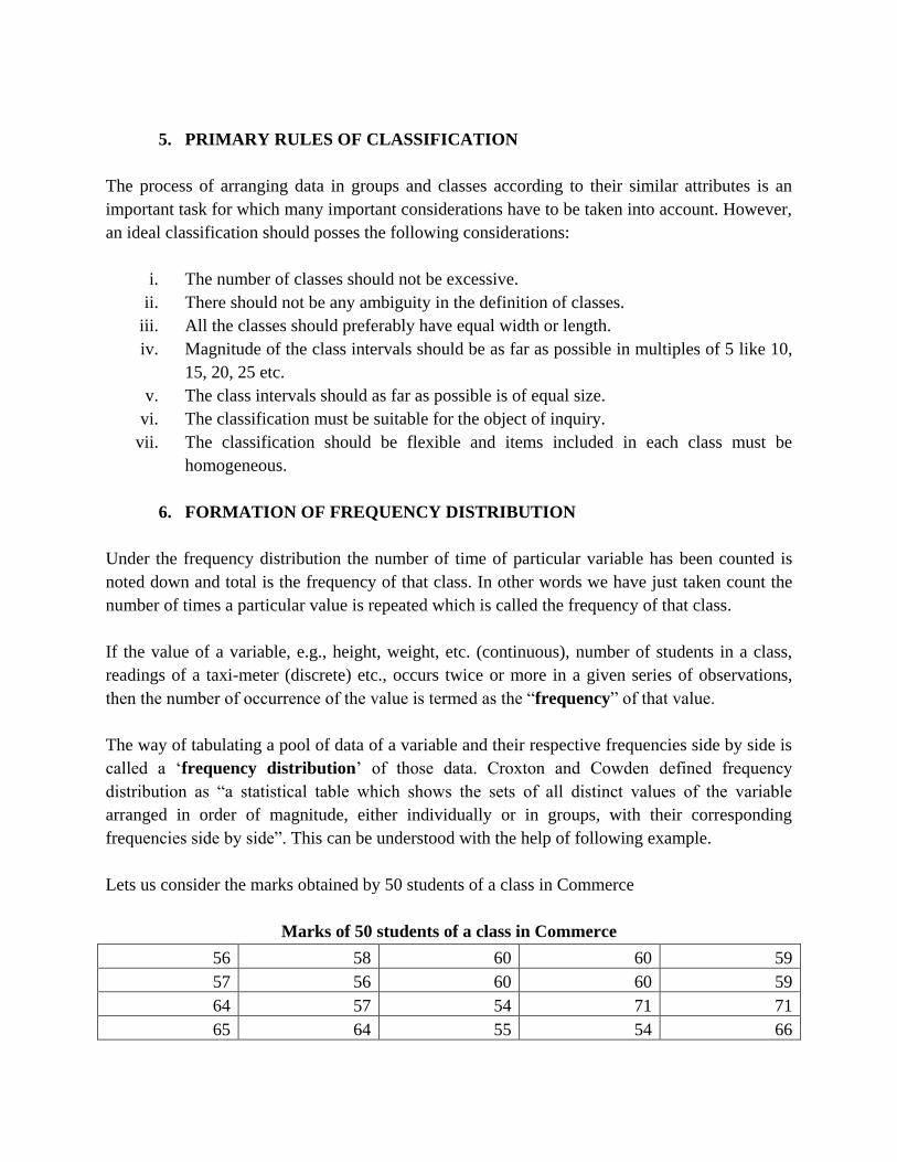
6. FORMATION OF FREQUENCY DISTRIBUTION

Under the frequency distribution the number of time of particular variable has been counted is

noted down and total is the frequency of that class. In other words we have just taken count the

number of times a particular value is repeated which is called the frequency of that class.

If the value of a variable, e.g., height, weight, etc. (continuous), number of students in a class,

readings of a taxi-meter (discrete) etc., occurs twice or more in a given series of observations,

then the number of occurrence of the value is termed as the “frequency” of that value.

The way of tabulating a pool of data of a variable and their respective frequencies side by side is

called a ‘frequency distribution’ of those data. Croxton and Cowden defined frequency

distribution as “a statistical table which shows the sets of all distinct values of the variable

arranged in order of magnitude, either individually or in groups, with their corresponding

frequencies side by side”. This can be understood with the help of following example.

Lets us consider the marks obtained by 50 students of a class in Commerce

Marks of 50 students of a class in Commerce

56 58 60 60 59

57 56 60 60 59

64 57 54 71 71

65 64 55 54 66

68 65 63 55 54

67 68 65 64 55

62 67 68 66 64

62 62 67 72 65

58 58 62 69 68

58 59 61 61 72

If the raw-data are arranged in either ascending, or, descending order of magnitude, we get a better way of

presentation, usually called an “array”.

Array of Marks shown in table

54 58 60 64 67

54 58 61 64 68

54 58 61 65 68

55 58 62 65 68

55 59 62 65 68

55 59 62 65 69

56 59 62 66 71

56 60 63 66 71

57 60 64 67 72

57 60 64 67 72

Now let us present the above data in the form of a simple (or, ungrouped) frequency distribution

using the tally marks. A tally mark is an upward slanted stroke (/) which is put against a value

each time it occurs in the raw data. The fifth occurrence of the value is represented by a cross

tally mark (\) as shown across the first four tally marks. Finally, the tally marks are counted and

the total of the tally marks against each value is its frequency.

Frequency Distribution

Marks Tally Marks Frequency

54 III 3

56 II 2

55 III 3

57 II 2

58 IIII 4

59 III 3

60 IIII 4

61 II 2

62 IIII 4

63 I 1

64 IIII 4

Total frequency - 50

6.1 FORMATION OF DISCRETE FREQUENCY DISTRIBUTION

The statistical series define as the two variable quantities can be arranged side by side so that

measurable difference in the one corresponds with measurable difference in the other, the result

is said to form a statistical series”. Statistical series may be either discrete or continuous. A

discrete series may be formed from items which are exactly measurable. For example, the

number of students getting exactly 40, 50, 60, 70 marks can be easily counted. But height or

weight cannot be measured with absolute accuracy.

Discrete Series

Marks Number of Series

40 12

50 15

60 16

70 7

6.2 FORMATION OF A CONTINUOUS FREQUENCY DISTRIBUTION

Although the continuous series shows with the number of students with height exactly 5′–6″

cannot be counted. Exact height will be either (5′–6″+0.01″), or, (5′–6″– 0.01″). Here, we are to

count the number of students whose heights fall between 5′–0″ to 5′–6″. Such series are known

as ‘continuous’ series. The following technical terms are important when a continuous frequency

distribution is formed or data classified according to class intervals.

Continuous Series

Height ( Inch) Number of Series

54-60 15

60-66 14

66-72 9

72-78 12

65 IIII 4

66 II 2

67 III 3

68 IIII 4

69 I 1

71 II 2

72 II 2

7. CLASS INTERVALS

The difference between upper and lower limit of a class is known as class interval. For example

in the class 100-200 the class interval is 100 (200 minus 100 = 100).

7.1 TYPES OF CLASS INTERVALS

There are different types of class intervals are given below:

i. Inclusive Type

ii. Exclusive Type

iii. Open End Type

iv. Unequal Class Interval

Class Intervals

Exclusive Type Inclusive Type Open-end Type Unequal Class Interval

10-15 60-69 0-50 0-20

15-20 70-79 50-100 20-50

20-25 80-89 100-150 50-100

25-30 90-99 150-200 100-200

30-35 100-109 200-250 200-450

35-40 110-119 250-over 450-650

The different type of Class-intervals shows in the above table by different series of intervals, first

the exclusive type like 10–15, 15–20. Similarly, 15 is included and 10 excluded (lower limit) in

“above 10 but not more than 15” class-interval. In the exclusive type the class-limits are

continuous, i.e., the upper-limit of one class-interval is the lower limit of the next class-interval

and class limits of a class interval coincide with the class boundaries of that class-interval. It is

suitable for continuous variable data and facilitates mathematical computations.

Similarly class-intervals inclusive types are like 60–69, 70–79, 80–89, etc. Here both the upper

and lower class-limits are included in the class-intervals, e.g., 60 and 69 both are included in the

class-interval 60–69. This is suitable for discrete variable data. There is no ambiguity to which

an item belongs but the idea of continuity is lost. To make it continuous, it can be written as

59.5–69.5, 69.5–79.5, 79.5–89.5, etc.

In ‘open-end’ class-interval either the lower limit of the first class interval or, upper limit of the

last class-interval, or, both are missing. It is difficult to determine the mid-values of the first and

last class intervals without an assumption. If the other closed class-intervals have equal width,

then we can assume that the open-end class-intervals also have the same common width of the

closed class-intervals. Grouped frequency distributions are kept open ended when there is limited

number of items scattered over a long interval. Unequal class-intervals are preferred only when

there is a great fluctuation in the data.

8. TABULATION

Tabulation may be defined as the systematic presentation of numerical data in rows or/and

columns according to certain characteristics. It is designed to simplify presentation of data for

purpose of analysis and statistical inferences. The purpose of a table is to simplify the

presentation and to facilitate comparisons. A statistical table may be a simple one or it may be a

complex one, depending upon number of variable incorporated into it. This table may be one

way or two ways or manifold. Following illustration is simple example of tabulation.

For example, during 2014-15, there were three faculties with 840 students in commerce, 660 in

science and only 50 students in management. The percentage of males is 40%, 25% and 20%

respectively in each subject stream. This data can be tabulated as follows

Faculty Number of students Total

Male Female

Commerce 336 504 840

Science 165 495 660

Management 100 400 500

Total 601 1399 2000

9. OBJECTIVE OF TABULATION

The main objectives of tabulation are stated below:

i. It simplifies complex data

ii. It carry out investigation

iii. It do comparison

iv. It locate omissions and errors in the data

v. It use space economically

vi. It helps in reference

10. TYPES OF TABLE

In a broad way tabulation of data can be either simple or complex. In a simple tabulation

information are related about one or groups or independent questions whereas in complex

tabulation the data or the information are in two or more categories and as such is meant to give

information about one or more sets of inter related questions. Tables may broadly classify into

three categories as follows:

i. Simple Table or One Way Table: In this type of table only one characteristic are

shown. One way table supplies answers to questions about one characteristic of data only.

Gender No. of respondents % percent age total

Male 110 55

Female 90 45

TOTAL 200 100

ii. Two Way Table or Double Table: Such tables give information about two interrelated

characteristics of a particular phenomenon.

Category Less no. of

students

% percentage

High no. of

students

% percentage

Commerce 130 65 400 76.92

Management 70 35 120 23.08

Total 200 100 520 100

iii. Three Way Table: If three interrelated phenomena are to be studied there would be

three way tables. A three way table can answer questions relating to three interrelated

problems.

It should be remembered that as the number of characteristics represented increases the

table becomes more and more confusing and as such normally not more than four

characteristics should be represented in the same table.

Category of Classes

B.Com M.Com

Low Middle High Low Middle High

Gender

Male 30 70 80 10 15 35

Female 40 50 110 20 25 20

TOTAL 70 120 190 30 40 55

11. CONTENTS OF A TABLE

i. Table number: Each table should be numbered should be easy identification and

future reference.

ii. Title: Every table should have a title which is generally given at the top of the table

in the center.

iii. Captions: A caption generally has a main heading and a number of small

subheadings.

iv. Stubs: It refers to the headings of the horizontal rows and return on the left hand side

of the row.

v. Body: It contains the statistical data which have to be presented.

vi. Headnote: It refers to the data contained in the major part of the table and it is placed

below the title of the table.

vii. Footnote: Footnotes are given below the table and are meant to clarify anything

which is not clear from the heading, title, stubs and caption.

12. BASIC PRINCIPLES OF TABULATION

i. Tables should be clear, concise & adequately titled.

ii. Every table should be distinctly numbered for easy reference.

iii. Column headings & row headings of the table should be clear & brief.

iv. Units of measurement should be specified at appropriate places.

v. Explanatory footnotes concerning the table should be placed at appropriate places.

vi. Source of information of data should be clearly indicated.

vii. The columns & rows should be clearly separated with dark lines.

viii. Demarcation should also be made between data of one class and that of another.

ix. Comparable data should be put side by side.

x. The figures in percentage should be approximated before tabulation.

xi. The alignment of the figures, symbols etc. should be properly aligned and

adequately spaced to enhance the readability of the same.

xii. Abbreviations should be avoided.

13. SORTING OF DATA

Sorting of data is the last process of tabulation. It is a time-consuming process when the data is

too large. After classification the data may be sorted using either of the following methods:

i. Manual method: It is done by hand with the help of giving tally marks for the

number of times each event has occurred. Next the total tally marks are counted. The

method is simple and suitable for limited data.

ii. Mechanical and electrical method: To reduce the sorting time mechanical devices

may be used. This is described as mechanical tabulation. For electrical tabulation data

should be codified first and then punched on card. For each data a separate card is

used. The punched cards are checked by a machine called ‘verifier’. Next the cards

are sorted out into different groups as desired by a machine called ‘sorter’. Finally,

the tabulation is done by using a tabulator. The same card may be sorted out more

than once for completing tables under different titles.

iii. Tabulation using electronic computer: It is convenient to use electronic computer

for sorting when (a) data are very large; (b) data have to be sorted for future use and

(c) the requirements of the table are changing. Such tabulation is less time-consuming

and more accurate than the manual method.

14. SUMMARY

Statistic is the branch of mathematics concerned with collection, classification, analysis, and

interpretation of numerical facts, for drawing inferences on the basis of their quantifiable

probability. It can be interpreting aggregates of data too large to be intelligible by ordinary

observation because such data tend to behave in the regular, predictable manner. However, the

numerical figures called ‘data’ obtained by counting, or, measurement. It means collection,

classification, presentation, analysis, comparison and meaningful interpretation of ‘raw data’.

Whereas, in advanced phenomena numbers of researcher were used advanced tools of statistics

with systematic manner. In addition, the efficient functioning of various classification and

tabulation tactics is shown in this module. In this module various methods of classification and

tabulation has been discussed in detail. The major prominence in this module is on discussing

statistical data classification and tabulation with suitable examples.