classification accuracy and consistency in uk high stakes
TRANSCRIPT

CLASSIFICATION ACCURACY AND CONSISTENCY IN GCSE AND A LEVEL EXAMINATIONS OFFERED BY THE ASSESSMENT AND
QUALIFICATIONS ALLIANCE (AQA) NOVEMBER 2008 TO JUNE 2009
Chris Wheadon & Ian Stockford April 2010
Ofqual/11/4823
This report has been commissioned by the Office of Qualifications and Examinations Regulation.

Classification accuracy and consistency in GCSE and A level examinations
Contents Page Summary 3 1. Overview 4 2. Background 4 2.1 The move from paper based whole script marking to electronic item
based marking 4 2.2 Accurate to within a grade? 5 2.3 Modern approaches to estimating classification consistency and accuracy 5 2.4 Measuring dimensionality 7 3. Method 8 3.1 Procedure 8 3.1.1 Models 8 3.1.2 IRT Classification 8 3.1.2.1 Conditional category probabilities 8 3.1.2.2 Estimation 8 3.1.3 Non-IRT Classification 9 3.1.4 Classification consistency 9 3.1.5 Classification accuracy 10 3.2 Units 10 3.2.1 Reasons for inclusion of units 10 3.2.2 A level units 10 3.2.3 GCSE units 11 4. Results 11 4.1 AS level units 11 4.1.1 Descriptive statistics 11 4.1.2 Dimensionality and model fit 13 4.1.3 Classification accuracy and consistency 13 4.1.4 PSYB1 and CHEM2 16 4.1.5 How far wrong could we be? 17 4.1.6 Classification to within a grade 18 4.1.7 Improving classification accuracy 20 4.2 GCSEs 23 4.2.1 Descriptive statistics 23 4.2.2 Dimensionality and model fit 26 4.2.3 Classification accuracy 26 4.2.4 Linear GCSEs with lower or higher than expected accuracy indices 28 4.2.5 Classification to within a grade 30 4.2.6 How important is it to classify candidates correctly on every unit or component of a composite qualification? 30 5. Discussion and Recommendations 31 5.1 Caveats 31 5.2 Summary of results 31 5.3 Assumptions and violations 32 5.4 Which index/model? 32 5.5 Qualification design 32 5.6 How can classification indices be used? 33 5.7 Are there any dangers with pursuing high classification indices? 34 5.8 Further research 34 5.9 Recommendations 34 References 36 Appendix A 38 Appendix B 42
2

Classification accuracy and consistency in GCSE and A level examinations
CLASSIFICATION ACCURACY AND CONSISTENCY IN GCSE AND A LEVEL EXAMINATIONS OFFERED BY THE ASSESSMENT AND
QUALIFICATIONS ALLIANCE (AQA) NOVEMBER 2008 TO JUNE 2009
SUMMARY The aim of this study was to investigate the classification accuracy and consistency in individual units of GCSE and A level examinations offered by the Assessment and Qualifications Alliance (AQA) from November 2008 to June 2009. As marking reliability has been considered extensively elsewhere the scope was limited to those units composed of objective, short answer or structured response test items which were considered to allow the assumption of reliable marking. Two models were used to derive the estimates: an IRT model; and the Livingston and Lewis procedure (1995). The assumptions of the IRT model are more stringent as they assume that parallel tests are equivalent in difficulty. As expected from this difference in assumptions and from the wider literature the indices were lower for the Livingston and Lewis procedure than for the IRT model. The results showed that, for the GCE and GCSE units analysed, at least 89 per cent of all candidates with a particular grade (other than the highest or lowest grade) have true scores either in that grade or immediately adjacent. For some units the figure is much higher than this, up to 100 per cent. There was more variation at GCSE than there was at GCE. The main reason for this was that the qualification criteria that governed the GCSEs modelled here were less restrictive than they were for GCE; as a result a GCSE could be comprised of anything from two to seven units. The length of the test was in proportion to the percentage of marks the unit accounted for in the total qualification. As a result there were GCSE units where the lowest maximum mark was lower than A level units and others where the highest maximum mark was higher. The mean grade boundary width, which is directly related to classification consistency and accuracy, accordingly shows greater variation for GCSE than for A levels. The GCSE qualification criteria have now been tightened, but still allow some variation in the number of units. The main issue found with classification and accuracy statistics is that they are population dependent; they reveal as much about the test-takers as they do about the tests themselves. Candidates whose true scores lie far to one side of the highest and lowest grade boundaries will always be correctly classified. As some A levels always attract a high-performing cohort they will also always be likely to achieve high classification indices. Classification indices on certain units may also need to be sacrificed in order to maintain standards in a qualification. As coursework outcomes rise, written outcomes may be reduced so that the overall qualification level outcomes are comparable over time. This may result in narrow grade boundaries in the tail of mark distributions with resulting low classification indices. This is inevitable, but undesirable, and has no bearing on the quality of the unit itself. There are instances, however, where classification indices serve a useful diagnostic purpose. They can reveal tests that are failing to discriminate as well as they should be, and tests that are mistargeted - either too easy or too hard. They can therefore, when used in conjunction with other indicators, form a useful part of the quality control and assurance procedures used in the development and delivery of qualifications.
3
Classification accuracy and consistency in GCSE and A level examinations
As the indices reveal little in themselves it is suggested that case studies of certain units could be shared between those with the expertise to interpret them so that a shared understanding may develop. These groups may include Ofqual, other awarding bodies or a group of assessment experts. This process would promote understanding of how indices are likely to vary between awarding bodies, between specification designs and subjects, and over time.
1. OVERVIEW National high-stakes examinations in England classify candidates into grades based on their marks. It is not unreasonable, therefore that users of those qualifications have an interest in statistics that directly address the issue of the accuracy and consistency of those classification decisions (Wiliam, 2009). These statistics, however, are not without issues and assumptions, which need to be explored before they are routinely reported. This research uses recent examination data to explore two approaches to measuring classification consistency and accuracy within single units of examinations. The classification accuracy and consistency at the qualification level, which may consist of multiple units, is beyond the scope of this project. As methods to estimate classification accuracy and consistency techniques are complex, the report assumes a basic knowledge of psychometric concepts.
2. BACKGROUND 2.1 The move from paper based whole script marking to electronic item based marking Awarding bodies have moved, to a greater or lesser extent, away from paper based marking of whole scripts to electronic item based marking. This development has two main benefits. The first is that, as items are randomly allocated to markers, the marking error has little effect at script level where there are a reasonable number of items. Markers could be considered to be interchangeable, and do not need to be explicitly modelled (Maris & Bechger, 2006). Secondly, a large amount of item level data is available, which increases the range of models that can be applied to enhance understanding of accuracy and consistency of grading.
4

Classification accuracy and consistency in GCSE and A level examinations
2.2 Accurate to within a grade? The last comprehensive study of classification consistency and accuracy (the terms were used interchangeably) of UK high-stakes examinations1 was undertaken over thirty years ago (Wilmott & Nuttall, 1975). This study suffered the disadvantage of small sample sizes, as the data were not readily available, along with the prevalence of optional questions in the design of the papers, which violated some key statistical assumptions. Nevertheless the authors estimated Cronbach’s alpha, and, using the look-up tables of grading reliability provided by Ebel (1965), concluded that the examinations (CSEs and O levels) were accurate to within plus or minus one grade at qualification level. The use of Cronbach’s coefficient alpha as the basis of the analysis meant that, where results differed between qualifications, they were unable to deduce the cause - the degree to which the tests were measuring more or less of a single underlying trait and the degree to which candidates were responding to tests in a reproducible manner. This uncertainty inevitably led them to the conclusion that the pursuit of reliability targets would lead to examinations focussed on measuring a single trait - the result would be that candidates would learn more about less and less,
It is crucial for those concerned with constructing examinations and tests to realize that reliability is a necessary, but not sufficient, condition for validity; striving to achieve reliability as an independent goal is simply a misdirection of effort. (Wilmott & Nuttall, 1975, p. 55)
Following this study the only brief flurry of interest in classification consistency and accuracy came with the discussion on the number of grades required for A levels (Cresswell, 1984). Cresswell cites the work of Pilliner (1969) who formulated the aspiration that 95 per cent of all candidates with a particular grade (other than the highest or lowest grade) should have true scores either in that grade, the one above, or the one below. He, along with Please (1971), Mitchelmore (1981) and Ward (1972), had come to this conclusion through the reasoning that unless an examination is perfectly reliable, some of those who lie to just one side of a grade will have true scores that fall the other side of it. As a consequence, no examination system can have an accuracy of better than plus or minus one grade - at the individual test level or the qualification level. The focus on the middle grades excludes those candidates who are at the extremes of the distribution and are likely to be correctly classified by any test with a reliability of greater than zero. While essentially arbitrary, as all targets are, the classification of 95 per cent of candidates to an accuracy of plus or minus one grade seems a useful point of reference.
2.3 Modern approaches to estimating classification consistency and accuracy Since 1975 the definitions of classification consistency and accuracy have been clarified. Classification consistency refers to the level of agreement between classifications based on two randomly parallel forms of a test (Livingston & Lewis, 1995). Classification accuracy refers to the degree to which observed classifications agree with those based on examinees’ true scores (Lee, Hanson, & Brennan, 2002; Livingston & Lewis, 1995). In general, the method for computing classification consistency indices depends on:
1 National curriculum assessment is not considered high-stakes here as the stakes are low for the candidates.
5

Classification accuracy and consistency in GCSE and A level examinations
Item types (dichotomous, polytomous, or complex - a combination of the two)
Types of scores (raw scores, scale scores, or composite scores over a set of multiple content categories)
Types of indices (overall or conditional classification consistency and accuracy indices)
Estimation of the true score distribution (distributional approach versus individual approach)
Different weights for items
Software available Key references to the available methods are detailed in Figure 1. The vast majority of item response theory (IRT) methods assume a single latent trait is being measured by any test. The IRT-based mixed format approach suggested by Lee, for example, assumes that parallel tests are equivalent in item difficulty. The non-IRT based approaches do not explicitly make this assumption, and therefore produce lower indices than the IRT-based approach (Lee, 2008; Lee et al., 2002). The different assumptions may suit some situations better than others. Integral to both techniques is fitting the observations to a model and unsurprisingly the fit of models may also differ. When fitting to the observed test scores in a non-IRT approach the four-parameter beta binomial model, for example, is known to outperform the two-parameter beta binomial model. However a three-parameter IRT-based approach has been found to provide the best fit of all (Lee et al., 2002). The best fit, however, does not necessarily translate into the best predictions (Hitchcock & Sober, 2004). The basic role of the models in estimating the classification indices is to estimate the latent score distribution and predict the observed score distribution (Lee et al., 2002). The three components of the models are: the estimated true score distributions, fitted observed score distributions and estimated conditional error variances, and these will exert considerable influence on the estimates of the classification indices (Lee et al., 2002).
6

Classification accuracy and consistency in GCSE and A level examinations
Model Test Type Procedure/Reference IRT Dichotomous Items Huynh (1990)
Schulz, Kolen, and Nicewander (1999) Lee, Hanson, and Brennan (2002)
Polytomous Items Wang, Kolen, and Harris (2000)
Mixed Format Lee (2008) Composite Score Knupp, Lee, and Ansley (2009)
Non-IRT Dichotomous Items Huynh (1976) Subkoviak (1976) Peng and Subkoviak (1980) Woodruff and Sawyer (1989) Hanson and Brennan (1990)
Polytomous Items Lee, Wang, Kim, and Brennan (2006)
Polytomous Items Peng and Subkoviak (1980) or Breyer and Lewis (1994)
Mixed Format Livingston and Lewis (1995) Lee, Brennan, Wan (2009) Composite Score Livingston and Lewis (1995)
Lee, Brennan, Wan (2009) Figure 1: Single-Administration Procedures for Estimating Classification Consistency and Accuracy (reproduced from Lee, 2009)
2.4 Measuring dimensionality There are two properties which describe the internal structure of any scale that is assumed to be unidimensional. The first property is the extent to which a single latent variable accounts for the variance observed in the data. This is equivalent to the variance explained by the first factor of a principal components analysis. The second property pertains to the proportion of variance in the secondary factors that are accounted for by the latent variable common to all factors (Cronbach, 1951; McDonald, 1999; Revelle, 1979). The higher the proportion of variance in the secondary factors explained by the dominant latent variable the more accurately an individual’s relative standing on that latent variable can be predicted. A coeffiecient omega has been suggested (Revelle, 2009a; Revelle, 2009b; Zinbarg, Revelle, Yovel, & Li, 2005), which can be interpreted as the square of the correlation between each factor score and the latent variable common to all factors in the infinite universe of factors of which the factor scores are a subset.
7

Classification accuracy and consistency in GCSE and A level examinations
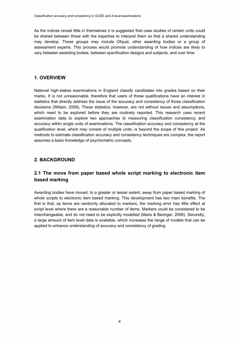
3. METHOD 3.1 Procedure 3.1.1 Models As the different models produce different estimates it was decided that two models would initially be applied for comparison purposes. The models applied are the IRT procedure outlined by Lee (2008) and the Livingston and Lewis procedure (1995). Both are suitable for mixed-format assessments. While software is available to calculate the outcomes (http://www.education.uiowa.edu/casma/) the authors developed their own routines for the estimation in R (R Development Core Team, 2009) with a view ultimately of integrating them into their data processing systems. It is hoped that these libraries will be released for general use in R. 3.1.2 IRT Classification 3.1.2.1 Conditional category probabilities IRT classification uses the probability that candidates of a given ability, theta, will answer correctly questions of a specified difficulty to calculate the probability of their achieving every possible score in a test. Due to the IRT assumption of conditional independence (that is every answer given is assumed to depend only on the latent trait being measured) the probability of candidates achieving these potential scores can be expressed by multiplication of probabilities for item responses for a given ability, theta. As there are many ways to achieve any score in a test the calculation is not straightforward (the interested reader can consult Lee (2008) and Kolen and Brennan (2004, p. 219) for details of the calculation). The true score of the candidate under IRT is equivalent to his/her expected score – the score candidates of a given theta are most likely to achieve. Once the true score and the probabilities of achieving all other scores have been determined for a candidate the probability of their score lying in the same category as that of their true score (classification accuracy), or the probability of consistent classification in a category over administrations (classification consistency), can be calculated. An example of these conditional category probabilities for a fictional assessment is given in Figure 2. 3.1.2.2 Estimation For pragmatic reasons the Rasch model was used to estimate theta and beta parameters; 2- and 3- parameter IRT models can fail to converge for the structured response assessments typical in the UK. The R package eRm: Extended Rasch Modelling (Mair & Hatzinger, 2009) was used to estimate item parameters with CML estimation and ability parameters with MML estimation.
8
Classification accuracy and consistency in GCSE and A level examinations
9
true score
pro
bab
ility
0.0
0.2
0.4
0.6
0.8
1.0
0 20 40 60 80 100
grade
Fail
E
D
C
B
A
Figure 2: Conditional category probabilities for an A level unit for different true scores 3.1.3 Non-IRT Classification The non-IRT approach selected for investigation is the procedure proposed by Livingston and Lewis (Livingston & Lewis, 1995). This technique is dependent on knowledge of the observed score distribution and the reliability of the test. To allow the examination of complex assessments (containing both dichotomous and polytomous items) an equivalent dichotomous test length is determined based upon the reliability of the actual administered test (as reported in Appendix B). The length of this dichotomous test is then used to determine a probability distribution of possible scores for each proportional true score level. These probability distributions of possible scores (defined by binomial distributions) can be used to assess the probability of classification into each category for each true score. The estimation of the observed scores with a four parameter beta binomial distribution provides a representation of the proportional true scores. This information, when combined with the probability distributions dependent on true score, allows determination of the classification accuracy and consistency. 3.1.4 Classification consistency The conditional classification consistency index is typically defined as the probability that examinees of a given ability are classified into the same category on independent administrations of two parallel forms of test. The summary statistic, the marginal classification index for all ability levels, can then be calculated by obtaining classification indices for every examinee and averaging them over all examinees.

Classification accuracy and consistency in GCSE and A level examinations
Another estimate of classification consistency is the k coefficient (Cohen, 1960). It is possible that, even with random scores, candidates will achieve the same grade. The k coefficient adjusts for the proportion of random consistency that can be expected. 3.1.5 Classification accuracy Classification accuracy is often evaluated by false positive and false negative error rates (Hanson & Brennan, 1990; Lee et al., 2002). The conditional false positive error rate is defined as the probability that an examinee is classified into a category that is higher than the examinee’s true category. The conditional false negative error rate is the probability that an examinee is classified into a category that is lower than an examinee’s true category. The true category can be determined by comparing the expected summed score of a candidate with the actual boundaries applied to the overall test. The probability that a candidate of given ability will then be classified into another category allows the false positive and false negative rates to be assessed. The accuracy is then determined by subtracting the incidence of false positives and false negatives from 1. Once again a summary statistic can be calculated by obtaining classification indices for every examinee and averaging them over all examinees.
3.2 Units 3.2.1 Reasons for inclusion of units Units for analysis were chosen on the basis of:
the availability of item-level data
relatively low item tariffs (to allow for the assumption of high marking reliability)
number of candidates
level of study (A level and GCSE) 3.2.2 A level units The structure of A levels has recently been changed so that an A level, with some exceptions, consists of four separate units. Two of these are AS units, which together form the AS qualification, and two are A2 units. A2 is not a qualification in its own right, but all four units form the A level qualification. After each unit has been graded the raw marks from that unit are translated onto a Uniform Mark Scale (UMS). A UMS scale is required as papers for a particular unit may vary slightly in levels of difficulty between examination series. This would lead to problems when aggregating scores for candidates sitting the same unit at different times. A mark of 45 in January 2009, for example, may represent the same level of achievement as a mark of 48 in summer 2009. The UMS is a common, or uniform, scale so that both 45 (from January) and 48 (from the summer) are translated to the same uniform mark and therefore have the same value when contributing to an overall grade (http://store.aqa.org.uk/over/stat_pdf/UNIFORMMARKS-LEAFLET.PDF). Given this new structure in A levels it is appropriate to analyse units from the new specifications which were first examined in June 2009. These are AS units. No A2 units have yet been examined from the new specifications and are therefore not included in the analysis.
10

Classification accuracy and consistency in GCSE and A level examinations
11
3.2.3 GCSE units From September 2009 most GCSE specifications became modular like A level rather than linear (but without the division into two levels). Therefore, assessments may be entered at different points during a candidate’s course of study. For example, a candidate following a two-year course leading to a GCSE qualification may enter one unit in June of Year 1, another in January of Year 2 and another in June of Year 2 (subject to the availability of the units at these times). Modular schemes normally allow candidates to re-take units if they wish. Under the old linear scheme all assessments had to be entered in the same examination series, e.g. June of Year 2. As in the case of A level, candidates’ results on individual modules (tests) in modular GCSE specifications will be translated onto a UMS scale. For this reason it was decided to consider results from a recent series for two GCSE specifications, Mathematics and Science, which were already modular before September 2009, and to draw comparisons with their linear counterparts. Unlike A levels, GCSEs have no standard design and can vary in features such as the number of units and the maximum uniform mark. Like A levels, the modes of assessment included in the qualification can vary. A selection of other linear assessments was also included in the analysis as they displayed interesting features.
4. RESULTS 4.1 AS level units 4.1.1 Descriptive statistics Most of the units analysed are comprised of a large number of low tariff questions (Table 1). Both Accounting units and the three Psychology units use some extended response questions and therefore the marking reliability of these units will influence the precision of the results that follow. The highest mark obtained varies from 52 (on a unit with a maximum of 60) to 98 (on a unit with a maximum of 100). If the rule of thumb that the standard deviation should be about 1/6 of the available marks is used then it would seem that the marks of candidates are reasonably well spread. The relatively low values for kurtosis would seem to accord with this impression. The skew reveals that the marks are more likely to be negatively skewed, implying that the units tend to be too easy for the candidature. It could be argued that it is more important to discriminate at the lower end of the scale with AS units as the more able candidates will probably progress to A2, at which point further discrimination can be achieved.

Classification accuracy and consistency in GCSE and A level examinations
Table 1: Descriptive statistics for AS level units
Specification Unit n items
highest item
score
highest test
score
maximum available
score mean mean (%) sd
sd (%) skew kurtosis
mean width of grade
boundary
mean width of grade boundary
(%)
ACCOUNTING ACCN1 4362 9 21 80 80 44.68 55.9 13.71 17.1 -0.34 0.10 5.50 6.9
ACCOUNTING ACCN2 6573 14 20 76 80 41.64 52.0 14.92 18.7 -0.40 -0.22 6.00 7.5
BIOLOGY BIOL1 23100 32 5 57 60 28.75 47.9 10.11 16.9 0.04 -0.61 4.50 7.5
BIOLOGY BIOL2 36608 46 6 78 85 43.04 50.6 13.35 15.7 -0.31 -0.45 5.75 6.8
CHEMISTRY CHEM1 12933 33 6 69 70 39.73 56.8 14.51 20.7 -0.32 -0.62 6.75 9.6
CHEMISTRY CHEM2 21747 54 6 98 100 48.47 47.5 21.27 21.3 -0.06 -0.91 9.00 9.0
COMPUTING COMP2 4070 31 6 56 60 24.86 41.4 9.95 16.6 0.40 -0.23 5.50 9.2
ELECTRONICS ELEC1 917 31 7 67 67 38.40 57.3 14.91 22.3 -0.20 -0.84 5.75 8.6
ELECTRONICS ELEC2 907 27 5 66 67 32.17 48.0 15.60 23.3 -0.01 -0.91 5.50 8.2
ENVS1 1754 22 8 52 60 25.92 43.2 8.01 13.4 0.12 -0.10 4.00 6.7 ENVIRONMENTAL STUDIES
ENVS2 2891 31 10 86 90 43.93 48.8 15.53 17.3 -0.08 -0.51 7.75 8.6 ENVIRONMENTAL STUDIES
HBIO1 1110 34 6 70 80 27.42 34.3 12.14 15.2 0.63 0.02 5.50 6.9 HUMAN BIOLOGY
HBIO2 1799 31 6 73 80 39.98 50.0 10.99 13.7 -0.08 -0.10 4.75 5.9 HUMAN BIOLOGY
PHYA1 14324 30 6 69 70 39.93 57.0 14.35 20.5 -0.29 -0.70 5.75 8.2 PHYSICS A
PHYA2 17220 28 6 70 70 42.92 61.3 15.61 22.3 -0.58 -0.61 6.75 9.6 PHYSICS A
PHYB2 1015 32 6 65 70 28.18 40.3 13.15 18.8 0.28 -0.54 5.00 7.1 PHYSICS B
PSYA1 35258 22 12 72 72 39.86 55.4 12.52 17.4 -0.23 -0.52 6.00 8.3 PSYCHOLOGY A
PSYA2 49286 19 12 72 72 34.41 47.8 13.64 18.9 0.00 -0.77 6.50 9.0 PSYCHOLOGY A
PSYB1 5892 21 10 57 70 33.62 48.0 9.24 13.2 -0.39 -0.18 4.25 6.1 PSYCHOLOGY B
SCIENCE IN SOCIETY SCIS1 1697 47 6 77 90 43.38 48.2 11.54 12.8 -0.16 0.07 4.75 5.2
12

Classification accuracy and consistency in GCSE and A level examinations
4.1.2 Dimensionality and model fit The average correlation between items varies between 0.1 for SCIS1 to 0.34 for ELEC2 while the general factor saturation (omega) varies from 0.64 for PSYB1 and ENVS1 to 0.88 for CHEM1 (Table 2). Generally the average inter-item correlation seems low, but the values of omega suggest that there are enough items for a general factor to emerge in each unit. This satisfies the assumption of unidimensionality required for the IRT approach. More precision, however, can be attributed to the results that follow for those units with a higher value of omega. It is interesting to note that SCIS1, with the second highest number of items, delivered the lowest inter-item correlations, while CHEM2, which contained far more items than CHEM1, also delivered lower inter-item correlations. For reference, reliability coefficients for these units can be found in appendix B. For the IRT model, the fit of the model was checked at the item level. Items were flagged as misfitting where the Outfit Mean Square value was greater than 1.2. These are detailed in Table 3. Table 2: Inter-item correlations and general factor saturation
Specification Unit average
r omega
ACCOUNTING ACCN1 0.29 0.68
ACCOUNTING ACCN2 0.27 0.70
BIOLOGY BIOL1 0.14 0.79
BIOLOGY BIOL2 0.15 0.75
CHEMISTRY CHEM1 0.24 0.88
CHEMISTRY CHEM2 0.23 0.74
COMPUTING COMP2 0.16 0.70
ELECTRONICS ELEC1 0.28 0.73
ELECTRONICS ELEC2 0.34 0.80
ENVIRONMENTAL STUDIES ENVS1 0.13 0.64
ENVIRONMENTAL STUDIES ENVS2 0.20 0.86
HUMAN BIOLOGY HBIO1 0.17 0.67
HUMAN BIOLOGY HBIO2 0.16 0.74
PHYSICS A PHYA1 0.26 0.80
PHYSICS A PHYA2 0.30 0.81
PHYSICS B PHYB2 0.22 0.73
PSYCHOLOGY A PSYA1 0.20 0.73
PSYCHOLOGY A PSYA2 0.24 0.83
PSYCHOLOGY B PSYB1 0.16 0.64
SCIENCE IN SOCIETY SCIS1 0.10 0.66
4.1.3 Classification accuracy and consistency As expected there is a close relationship between the results from the two models, but those from the Livingston-Lewis approach, are consistently lower. The Livingston-Lewis approach has less restrictive assumptions, and allows the difficulty of the hypothetically parallel tests to differ. Under the IRT-model the classification accuracy varies from 0.55 for PSYB1 to 0.73 for CHEM2 (Table 3). Under the Livingston-Lewis approach they range from 0.53 to 0.69. The
13

Classification accuracy and consistency in GCSE and A level examinations
14
consistency indices for both models are lower as they represent the sums of the squares of the probability of classification into each grade. As expected, the classification indices are closely related to grade boundary width. Figure 3 shows the relationship between classification accuracy and grade boundary width in these units. CHEM2 has the widest grade boundaries, the highest standard deviation and the highest classification accuracy. PSYB1 has amongst the lowest standard deviation and narrowest grade boundaries. Further exploration of these two units sheds more light on why classification indices differ and is performed in the following sections.
average grade boundary width
cla
ssifi
catio
n a
ccu
racy
0.55
0.60
0.65
0.70
4 5 6 7 8 9
specification
ACCOUNTING
BIOLOGY
CHEMISTRY
COMPUTING
ELECTRONICS
ENVIRONMENTAL STUDIES
HUMAN BIOLOGY
PHYSICS A
PHYSICS B
PSYCHOLOGY A
PSYCHOLOGY B
SCIENCE IN SOCIETY
Figure 3: The relationship between classification accuracy and grade boundary width for new AS units under the IRT model

Classification accuracy and consistency in GCSE and A level examinations
Table 3: Classification accuracy and consistency
IRT Livingston and Lewis
Unit AccuracyFalse
PositiveFalse
Negative Consistency Kappa ChanceMisfitting
items AccuracyFalse
PositiveFalse
Negative Consistency Specification
ACCOUNTING ACCN1 0.61 0.17 0.22 0.53 0.37 0.28 1 0.53 0.22 0.25 0.36
ACCOUNTING ACCN2 0.62 0.17 0.21 0.54 0.39 0.26 3 0.56 0.22 0.22 0.40
BIOLOGY BIOL1 0.60 0.20 0.20 0.51 0.41 0.19 1 0.58 0.21 0.21 0.40
BIOLOGY BIOL2 0.63 0.19 0.18 0.54 0.44 0.18 3 0.61 0.18 0.21 0.42
CHEMISTRY CHEM1 0.67 0.16 0.17 0.57 0.49 0.17 3 0.64 0.19 0.17 0.45
CHEMISTRY CHEM2 0.73 0.14 0.14 0.64 0.56 0.18 7 0.69 0.16 0.15 0.52
COMPUTING COMP2 0.60 0.20 0.20 0.49 0.40 0.18 2 0.54 0.23 0.22 0.32
ELECTRONICS ELEC1 0.67 0.17 0.16 0.60 0.50 0.20 5 0.62 0.21 0.17 0.44
ELECTRONICS ELEC2 0.70 0.15 0.15 0.63 0.54 0.20 4 0.65 0.19 0.16 0.49
ENVIRONMENTAL STUDIES ENVS1 0.57 0.20 0.23 0.48 0.34 0.24 1 0.54 0.22 0.25 0.34
ENVIRONMENTAL STUDIES ENVS2 0.64 0.17 0.19 0.54 0.44 0.19 1 0.61 0.20 0.19 0.42
HUMAN BIOLOGY HBIO1 0.67 0.16 0.18 0.60 0.45 0.30 3 0.65 0.16 0.19 0.50
HUMAN BIOLOGY HBIO2 0.59 0.19 0.22 0.51 0.39 0.23 3 0.58 0.19 0.23 0.40
PHYSICS PHYA1 0.67 0.17 0.16 0.59 0.49 0.19 2 0.64 0.19 0.17 0.47
PHYSICS A PHYA2 0.68 0.16 0.16 0.60 0.50 0.19 6 0.66 0.18 0.16 0.47
PHYSICS B PHYB2 0.64 0.18 0.18 0.56 0.46 0.19 2 0.62 0.20 0.17 0.45
PSYCHOLOGY A PSYA1 0.60 0.19 0.21 0.51 0.40 0.19 0 0.56 0.23 0.21 0.36
PSYCHOLOGY A PSYA2 0.60 0.19 0.20 0.52 0.41 0.19 2 0.57 0.23 0.20 0.38
PSYCHOLOGY B PSYB1 0.55 0.22 0.23 0.47 0.35 0.19 1 0.54 0.23 0.23 0.35
SCIENCE IN SOCIETY SCIS1 0.58 0.21 0.22 0.49 0.39 0.18 1 0.56 0.22 0.22 0.37
15

Classification accuracy and consistency in GCSE and A level examinations
16
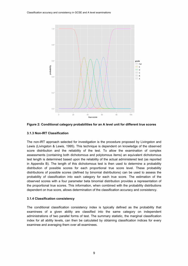
4.1.4 PSYB1 and CHEM2 The descriptive statistics show that the CHEM2 marks have a much flatter distribution than the PSYB1 marks (the %sd for CHEM 2 is 21.3 compared to 13.2 for PSYB1). This is shown visually in Figure 4, which also superimposes the grade boundaries onto the mark distributions. While PSYB1 peaks around the central grade, CHEM2, for some unexplained reason, has two peaks. This reduces the density of candidates in CHEM2 around the central grades. Figure 5 shows the impact these distributions have on classification accuracy. The thickness and colour of the lines is proportional to the number of candidates on each mark. The accuracy for CHEM2 shows the characteristic U shapes around the boundaries. Candidates on the cut-scores have a 50-50 chance of being classified accurately; in other words when a true score lies just to one side of the boundary there is a high likelihood of achieving a score just the other side of that boundary, but only that boundary. For PSYB1, however, the chances are closer to 1 in 3. Not only are candidates likely to be classified into the adjacent category, but also into other grade categories for the unit. The width between most of the PSYB1 boundaries is 4 marks; between the grade A and B boundaries it is 5 marks. This allows grade A candidates to be clearly separated from the grade C boundary and the accuracy to rise to 0.45 near the grade A boundary. Unfortunately for PSYB1 the peak of the distribution is centred around the grade B and C boundaries where the marginal accuracy is at its lowest. This results in low values for the summary classification indices.
observed score
dens
ity
0.00
0.01
0.02
0.03
0.04
10 20 30 40 50
observed score
dens
ity
0.000
0.005
0.010
0.015
20 40 60 80
Figure 4: The mark distributions with grade boundaries superimposed for PSYB1 (left) and CHEM2 (right)
Classification accuracy and consistency in GCSE and A level examinations
17
true score
accu
racy
0.4
0.5
0.6
0.7
0.8
0.9
1.0
0 10 20 30 40 50
frequency
0
10
20
30
40
true score
accu
racy
0.5
0.6
0.7
0.8
0.9
1.0
0 20 40 60 80
frequency
0
5
10
15
20
25
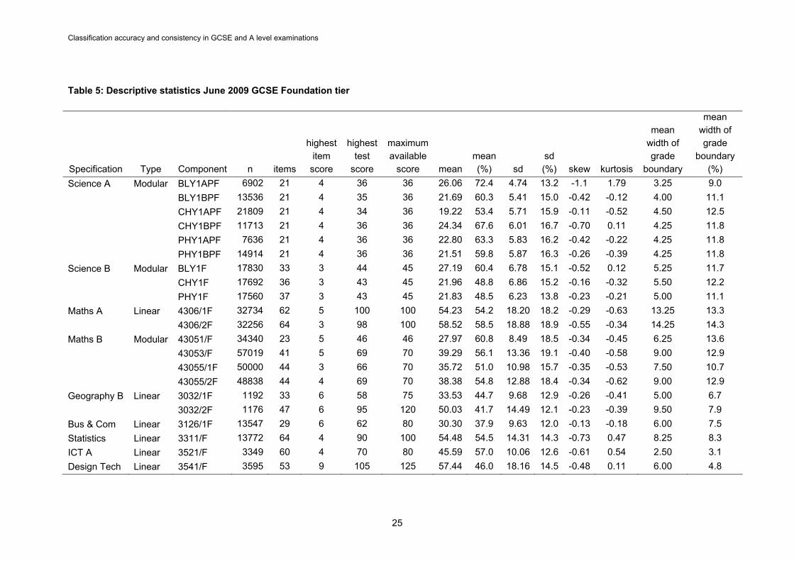
Figure 5: Classification accuracy for PSYB1 (left) and CHEM2 (right) under the IRT model 4.1.5 How far wrong could we be? While the classification accuracy index indicates the rate of correct classifications, and therefore the rate of misclassifications, it does not clearly reveal the severity of any misclassification. Figure 6 provides a visualisation of the IRT-based statistics which form the basis of the classification consistency indices. Each cell shows the probability of achieving that combination of grades on two hypothetical parallel forms (therefore representing consistency rather than accuracy). The diagonal represents the probability of consistent classification. For CHEM2 the probability of being classified more than one grade distant on two occasions is zero. For PSYB1 there is a chance (albeit extremely small) of being classified with a B on one administration and an E on another.

Classification accuracy and consistency in GCSE and A level examinations
18
U
E
D
C
B
A
00000.030.21
0000.030.060.03
000.030.060.030
00.030.060.0300
0.030.070.03000
0.180.030000
U E D C B A
U
E
D
C
B
A
000.010.020.040.21
00.010.020.030.030.04
00.020.040.040.030.02
0.010.040.050.040.020.01
0.040.060.040.020.010
0.070.040.01000
U E D C B A
Figure 6: Classification consistency on two separate administrations for PSYB1 (left) and CHEM2 (right) under the IRT model. Each cell shows the probability of achieving that combination of grades on two hypothetical parallel forms. 4.1.6 Classification to within a grade In order to create a summary statistic for the severity of misclassification it is useful to return to Pillner’s aspiration. This aspiration was that 95 per cent of all candidates with a particular grade (other than the highest or lowest grade) should have true scores either in that grade or the grades immediately adjacent. Pillner’s statistic can be easily calculated from the IRT-based marginal classification accuracy figures as presented in Table 4. This table shows that the lowest percentage accuracy to within a grade is 89 per cent for ACCN1, closely followed by PSYB1. For CHEM2, as expected from the preceding analysis, the figure is close to 100 per cent (the very small chance of being classified further than one grade from the true grade is obscured in Figure 6 by the rounding to 2 decimal places). The classification to within a grade appears relatively less successful for ACCN1 than would be expected from the preceding classification indices and from consideration of Figure 3. Figure 7 reveals that the peak of the distribution for this unit is centred around the grade E boundary. The large proportion of candidates who fall some distance to the left of this boundary have little chance of achieving a grade E, so they are classified accurately. The accuracy to within a grade summary statistic, however, only considers those candidates in the central grades neglecting this large number of correctly classified but low scoring candidates. As these correctly classified candidates are ignored using this analysis the measure of accuracy to within a grade is artificially low.

Classification accuracy and consistency in GCSE and A level examinations
Table 4: IRT estimation of the proportion of candidates with a particular grade (other than the highest or lowest grade) with true scores either in that grade, or the one adjacent
observed score
..de
nsi
ty..
0.000
0.005
0.010
0.015
0.020
0.025
0.030
10 20 30 40 50 60 70
true score
accu
racy
0.4
0.5
0.6
0.7
0.8
0.9
1.0
0 20 40 60
frequency
0
10
20
30
40
Specification Unit
Accuracy plus /
minus one grade
ACCOUNTING ACCN1 0.89
ACCOUNTING ACCN2 0.92
BIOLOGY BIOL1 0.92
BIOLOGY BIOL2 0.95
CHEMISTRY CHEM1 0.98
CHEMISTRY CHEM2 0.99
COMPUTING COMP2 0.96
ELECTRONICS ELEC1 0.95
ELECTRONICS ELEC2 0.95
ENVIRONMENTAL STUDIES ENVS1 0.90
ENVIRONMENTAL STUDIES ENVS2 0.97
HUMAN BIOLOGY HBIO1 0.93
HUMAN BIOLOGY HBIO2 0.91
PHYSICS PHYA1 0.96
PHYSICS A PHYA2 0.97
PHYSICS B PHYB2 0.93
PSYCHOLOGY A PSYA1 0.94
PSYCHOLOGY A PSYA2 0.94
PSYCHOLOGY B PSYB1 0.90
SCIENCE IN SOCIETY SCIS1 0.91
Figure 7: ACCN1 grade boundaries and classification accuracy
19

Classification accuracy and consistency in GCSE and A level examinations
20
Whether candidates in the extreme categories should be considered in a summary statistic is an interesting question; not including them should make the indices less responsive to changes in the ability of different cohorts of candidates. The question is perhaps subsumed by a bigger issue, however. Why are nearly half of the candidates for ACCN1 failing it? This is an extremely unusual situation; most AS units have failure rates closer to 20 per cent. The qualitative judgements of the awarding committee suggest that the boundaries are appropriate but what if they were not? If these grade boundaries are not in the right place then what meaning does an index of classification accuracy have? This example highlights a key assumption of these analyses; that the grade boundaries are appropriate to start with. 4.1.7 Improving classification accuracy To investigate methods of improving classification accuracy, units CHEM2 and PSYB1 are considered again. One way of improving the accuracy is to provide more information on candidates’ ability. The difference between the information available for CHEM2 and PSYB1 is shown by Rasch person-item maps (Figures 8 and 9). A person item map shows the ability of the candidates on the same scale as the difficulty of the items. Ideally the distribution of item difficulty should match the distribution of person ability. The person-item map for PSYB1 (figure 8) shows that the low-tariff items in particular are relatively easy for this population. This reduces the information that each produces. Items with longer tariffs (B2a and B2d) display disordered thresholds at their extremes. This implies that markers are reluctant to award the highest marks, again restricting discrimination. The CHEM2 person-item map, however, shows a high density of items with a range of tariffs located at all levels of ability. This increases the information available on every candidate and maximises the discrimination and grade boundary width. Harder questions, a more clearly specified mark scheme and better use of the range of marks within questions may be the solution for PSYB1. For PSYB1 it would seem that the negative skew of the mark distribution and the low classification indices are related. Negative skew does not always lead to high levels of misclassification, however. The Physics A papers (PHYA1, PHYA2) are negatively skewed; but a high proportion of candidates lie far to the right of the grade A boundary where they have little chance of failing to be classified as grade A candidates.

Classification accuracy and consistency in GCSE and A level examinations
C.3.d
C.3.c
B.2.b.ii
C.3.g
B.2.d
B.2.a
A.1.d
A.1.a
B.2.b.i
C.3.i.ii
C.3.e
C.3.h
A.1.c
C.3.f.ii
A.1.b.i
C.3.f.i
A.1.b.ii
B.2.c
C.3.b
C.3.i.i
C.3.a
-2 -1 0 1 2
Latent Dimension
2 1
1 2
1 2
2 1
1 3 25 4 6 7 8 10 9
1 2
1 2 3 4 5 6 7 1098
2 1 3
1 2 3
2 1
1 2
1 2 3
1 2 3 4
1
1
1
2 1
1 3 2
1 2
1
1 2
*
*
*
**
*
**
Person-Item Map
PersonParameter
Distribution
Figure 8: Rasch Person-Item map for PSYB1
21

Classification accuracy and consistency in GCSE and A level examinations
A.9.cA.4.d.iiA.1.d.iA.8.c
A.1.d.iiA.6.a
B.11.bA.5.c.iv
A.8.aA.6.b
A.5.c.iiA.7.c.iA.3.b
A.2.c.iA.3.a.ivB.10.bB.10.aA.2.b.iiA.2.c.iiB.11.aA.4.a
A.5.a.iiiA.5.c.iiiA.5.b.iA.5.c.iA.5.a.iiA.4.c.iA.8.dA.1.cA.6.c
A.2.b.iA.8.b
A.2.a.iA.2.c.iii
A.7.bA.2.a.iiiA.5.b.iiA.5.b.iiiB.10.cA.4.b
B.11.cA.4.d.iA.9.bA.1.a
A.7.c.iiA.3.a.iiA.3.a.iii
A.9.aA.5.a.iA.7.a
A.2.a.iiA.4.c.ii
A.1.bA.3.a.i
-5 -4 -3 -2 -1 0 1 2 3 4 5
Person-Item Map
PersonParameter
Distribution
Latent Dimension
11
111
11 4 2 3 5 6
11
1 21
2 11
11 2
1 2 3 5 41 2 3
11 2
42 31 51 2
1 21
2 111
11 4 23
1 21 2
11 2
1 2 31 2
23 4 513 1 2
2 11
2 1 4 31 2
211
3 2 11
11
111
11
11 2
1
**
22

Classification accuracy and consistency in GCSE and A level examinations
23
Figure 9: Rasch person-item map for CHEM2

Classification accuracy and consistency in GCSE and A level examinations
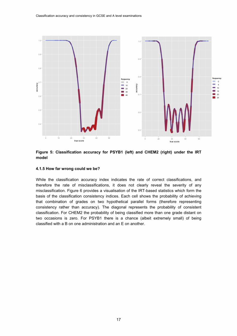
4.2 GCSEs To allow investigation of a more diverse range of qualification formats the analysis was extended to examine a selection of GCSE qualifications as outlined in section 3.2.3. In the interest of conciseness, this analysis is presented solely for the IRT based approach. 4.2.1 Descriptive statistics The descriptive statistics for GCSEs (tables 5 and 6) show more variation than those for A levels. The lowest maximum mark is lower (36 compared to 60) while the highest maximum mark is higher (125 compared to 100). The mean grade boundary width accordingly shows greater variation than for A levels with a low of 2.5 (compared to 4) and a high of 14.25 (compared to 9). Although the higher tier has to classify candidates into one more category than the foundation tier (A*,A,B,C,D,E for higher tier and C,D,E,F,G for foundation tier), the maximum marks available are often the same. As a result the mean width of the higher tier boundaries is narrower than that of the foundation tier boundaries. In Science A, for example, the mean width of the foundation tier boundaries across all units is more than one mark wider than that of the higher tier units (4.08 compared to 2.83). This could be the result of a historic anomaly as the grade E boundary at higher tier was introduced at a late stage in the development of GCSEs to reduce the incidence of candidates failing the higher tier completely. As such it is still considered to be an ‘allowed’ boundary with somewhat less currency than the others. The Higher tier is targeted only at A*-D. The reason for the greater variation in the design of GCSE units than for A level units is that the qualification criteria specified by the Qualifications and Curriculum Development Agency and regulated by Ofqual are less restrictive. A qualification can be made up of different numbers of units and/or components with different weightings. Unlike A levels the number of units is not specified. Across all the specifications investigated, the Science A units have the lowest maximum marks but each one only comprises 12.5 per cent of the marks of the total qualification. In contrast the Statistics component 3311/F comprises 75 per cent of the marks of the total qualification.
24
Classification accuracy and consistency in GCSE and A level examinations
Table 5: Descriptive statistics June 2009 GCSE Foundation tier
Specification Type Component n items
highest item
score
highest test
score
maximum available
score mean mean (%) sd
sd (%) skew kurtosis
mean width of grade
boundary
mean width of grade
boundary (%)
Modular BLY1APF 6902 21 4 36 36 26.06 72.4 4.74 13.2 -1.1 1.79 3.25 9.0 Science A
BLY1BPF 13536 21 4 35 36 21.69 60.3 5.41 15.0 -0.42 -0.12 4.00 11.1
CHY1APF 21809 21 4 34 36 19.22 53.4 5.71 15.9 -0.11 -0.52 4.50 12.5
CHY1BPF 11713 21 4 36 36 24.34 67.6 6.01 16.7 -0.70 0.11 4.25 11.8
PHY1APF 7636 21 4 36 36 22.80 63.3 5.83 16.2 -0.42 -0.22 4.25 11.8
PHY1BPF 14914 21 4 36 36 21.51 59.8 5.87 16.3 -0.26 -0.39 4.25 11.8
Modular BLY1F 17830 33 3 44 45 27.19 60.4 6.78 15.1 -0.52 0.12 5.25 11.7 Science B
CHY1F 17692 36 3 43 45 21.96 48.8 6.86 15.2 -0.16 -0.32 5.50 12.2
PHY1F 17560 37 3 43 45 21.83 48.5 6.23 13.8 -0.23 -0.21 5.00 11.1
Linear 4306/1F 32734 62 5 100 100 54.23 54.2 18.20 18.2 -0.29 -0.63 13.25 13.3 Maths A
4306/2F 32256 64 3 98 100 58.52 58.5 18.88 18.9 -0.55 -0.34 14.25 14.3
Modular 43051/F 34340 23 5 46 46 27.97 60.8 8.49 18.5 -0.34 -0.45 6.25 13.6 Maths B
43053/F 57019 41 5 69 70 39.29 56.1 13.36 19.1 -0.40 -0.58 9.00 12.9
43055/1F 50000 44 3 66 70 35.72 51.0 10.98 15.7 -0.35 -0.53 7.50 10.7
43055/2F 48838 44 4 69 70 38.38 54.8 12.88 18.4 -0.34 -0.62 9.00 12.9
Linear 3032/1F 1192 33 6 58 75 33.53 44.7 9.68 12.9 -0.26 -0.41 5.00 6.7 Geography B
3032/2F 1176 47 6 95 120 50.03 41.7 14.49 12.1 -0.23 -0.39 9.50 7.9
Linear 3126/1F 13547 29 6 62 80 30.30 37.9 9.63 12.0 -0.13 -0.18 6.00 7.5 Bus & Com
Statistics Linear 3311/F 13772 64 4 90 100 54.48 54.5 14.31 14.3 -0.73 0.47 8.25 8.3
Linear 3521/F 3349 60 4 70 80 45.59 57.0 10.06 12.6 -0.61 0.54 2.50 3.1 ICT A
Design Tech Linear 3541/F 3595 53 9 105 125 57.44 46.0 18.16 14.5 -0.48 0.11 6.00 4.8
25

Classification accuracy and consistency in GCSE and A level examinations
26
Table 6: Descriptive statistics June 2009 GCSE Higher tier
Specification Type Component n items
highest item
score
highest test
score
maximum available
score mean mean (%) sd
sd (%) skew kurtosis
mean width of grade
boundary
mean width of grade
boundary (%)
Science A Modular BLY1APH 11282 30 4 36 36 24.76 68.8 5.95 16.5 -0.49 -0.12 2.80 7.8
BLY1BPH 20692 30 4 36 36 26.02 72.3 5.06 14.1 -0.61 0.30 2.60 7.2
CHY1APH 37100 30 4 36 36 23.41 65.0 6.07 16.9 -0.25 -0.52 3.00 8.3
CHY1BPH 18635 30 4 36 36 21.52 59.8 5.14 14.3 -0.07 -0.36 3.00 8.3
PHY1APH 10412 30 4 36 36 23.05 64.0 4.97 13.8 -0.18 -0.05 2.80 7.8
PHY1BPH 22609 30 4 36 36 23.09 64.1 5.75 16.0 -0.13 -0.44 2.80 7.8
Science B Modular BLY1H 45942 22 4 44 45 28.37 63.0 6.67 14.8 -0.25 -0.41 4.20 9.3
CHY1H 45740 25 4 44 45 25.27 56.2 8.12 18.0 -0.22 -0.63 4.80 10.7
PHY1H 44233 34 2 44 45 25.58 56.8 7.57 16.8 -0.30 -0.54 4.80 10.7
Maths A Linear 4306/1H 23321 44 6 100 100 59.62 59.6 18.68 18.7 -0.11 -0.55 13.20 13.2
4306/2H 23273 42 6 100 100 56.83 58.6 19.02 19.0 0.04 -0.60 13.60 13.6
Maths B Modular 43051/H 37580 22 5 46 46 25.50 55.4 8.80 19.1 0.14 -0.66 6.60 14.3
43053/H 54730 30 5 70 70 33.80 48.3 14.51 20.7 0.33 -0.59 9.20 13.1
43055/1H 65113 39 3 70 70 37.55 53.6 12.30 17.6 0.36 -0.36 8.40 12.0
43055/2H 64984 26 6 70 70 36.91 52.7 13.32 19.0 0.26 -0.49 8.80 12.6
Geography B Linear 3032/1H 2042 28 6 72 75 45.37 60.5 10.49 14.0 -0.23 -0.25 5.80 7.7
3032/2H 2044 31 9 104 120 59.80 49.8 17.32 14.4 -0.10 -0.39 9.20 7.7
Bus & Com Linear 3126/1H 13114 20 7 74 80 45.90 57.4 8.75 10.9 -0.22 0.15 9.40 11.8
Statistics Linear 3311/H 20591 57 6 114 100 63.83 63.8 17.31 17.3 0.04 -0.39 11.80 11.8
ICT A Linear 3521/H 9447 55 5 77 80 56.09 70.1 8.08 10.1 -0.50 0.38 4.40 5.5
Design Tech Linear 3541/H 5176 32 23 123 125 73.75 59.0 18.62 14.9 -0.16 -0.44 9.60 7.7

Classification accuracy and consistency in GCSE and A level examinations
4.2.2 Dimensionality and model fit Of particular interest in the dimensionality analyses was the particularly low general factor saturation for the Science A units (Table 7). The average correlations between items were similar to those in the longer Science B units, but the general factor saturation was lower. While these two specifications are designed to measure the same assessment objectives and skills the Science B tests are longer and comprise greater proportions of the total qualification. It would seem that the Science A tests are too short for a general factor to clearly emerge. The results that follow for these tests should therefore be interpreted with caution. Other GCSE units and components showed similar levels of general factor saturation to the A level units. Table 7: General factor saturation for Science A and Science B
Specification Unit average
r omega
Science A BLY1APF 0.11 0.55
BLY1APH 0.12 0.70
BLY1BPF 0.09 0.53
BLY1BPH 0.09 0.60
CHY1APF 0.08 0.52
CHY1APH 0.12 0.59
CHY1BPF 0.12 0.66
CHY1BPH 0.08 0.57
PHY1APF 0.12 0.60
PHY1APH 0.08 0.62
PHY1BPF 0.10 0.62
PHY1BPH 0.11 0.76
Science B BLY1F 0.12 0.71
BLY1H 0.11 0.62
CHY1F 0.12 0.74
CHY1H 0.18 0.70
PHY1F 0.09 0.62
PHY1H 0.13 0.81
The number of misfitting questions was occasionally high, with 14 noted for Mathematics A 4306/1F. 4.2.3 Classification accuracy As expected, the greater variation in design of GCSEs means there is a greater variation in the classification indices (Figures 10 and 11). At one extreme the short Science A units have a classification accuracy of between 0.51 and 0.68 on the foundation tier and of between 0.46 and 0.55 on the higher tier. At the other extreme, the Maths A components with 100 raw marks available have a classification accuracy of between 0.74 and 0.78 on the foundation tier and between 0.73 and 0.77 on the higher tier. Once again the relationship between grade boundary width and accuracy is strong; but Figures 10 and 11 show that the linear GCSE units (from Maths A, Geog B, Design Tech, ICT A, Stats and Bus & Com specifications) with
27

Classification accuracy and consistency in GCSE and A level examinations
the exception of Maths A, are more variable in their accuracy. More detailed tables are presented in Appendix A.
average grade boundary width
cla
ssifi
catio
n a
ccu
racy
0.55
0.60
0.65
0.70
0.75
4 6 8 10 12 14
specification
BusCom
Design Tech
Geog B
ICT A
Maths A
Maths B
Science A
Science B
Stats
Figure 10: Classification accuracy for GCSE foundation tier November 2008 to June 2009
28

Classification accuracy and consistency in GCSE and A level examinations
average grade boundary width
cla
ssifi
catio
n a
ccu
racy
0.50
0.55
0.60
0.65
0.70
0.75
4 6 8 10 12
specification
BusCom
Design Tech
Geog B
ICT A
Maths A
Maths B
Science A
Science B
Stats
Figure 11: Classification accuracy for GCSE higher tier November 2008 to June 2009 4.2.4 Linear GCSEs with lower or higher than expected accuracy indices Figure 12 shows the raw mark distribution of four of the outlying foundation tier GCSE components from Figure 10. The ICT component 3521/F has a higher than expected accuracy index as it has large proportions of candidates in the extreme categories who are therefore easily classified. The Statistics component 3311/F has a higher than expected accuracy index as it has a large proportion of candidates whose performance greatly exceeds that required for a grade A. The Design and Technology component 3541/F has a higher than expected accuracy index as it has a large proportion of candidates who performance is far worse than required for a grade G. The Geography component 3032/2F has wide grade boundaries, but fewer candidates at the extremes. Despite having a relatively healthy spread of marks and reasonably placed and relatively wide grade boundaries it fails to achieve the accuracy indices of other units with similar characteristics. This is not due to an inherent flaw in the quality of the unit; rather it is due to the interaction between grade boundary placement and the accuracy and consistency indices. This interaction should be taken into account when accuracy and consistency indices are examined.
29

Classification accuracy and consistency in GCSE and A level examinations
30
All of these components could achieve higher classification and accuracy indices if the grade boundaries were drawn in different locations. There is a tension, however, between the need to maintain standards over time and the desire to achieve high classification and accuracy indices on every component. The Design and Technology component, for example, represents only 40 per cent of the total marks of the qualification; the other 60 per cent is composed of coursework. Coursework grade boundaries are fixed for the life of a qualification; outcomes therefore tend to increase over the life of a specification. The only way to keep qualification outcomes in line with previous outcomes is to grade the written papers severely. This has led to narrow grade boundaries located in the tail of the mark distribution. ICT A also has 60 per cent coursework; other factors may have caused the compression of the grade boundaries which in this case leads to higher than expected accuracy due to the high proportions of candidates achieving the extreme grades. The impact of coursework on the other two specifications should be less pronounced as it comprises only 25 per cent of the total marks in each case.
observed score
de
nsi
ty
0.0
observed score
de
nsi
ty
0.000
0.005
0.010
0.015
0.020
0.025
0.030
0 20 40 60 80
ICT A, 3521/F Statistics, 3311/F
0
0.0
0.0
0.0
0.0 4
3 2
1
10 20 30 40 50 60 70
observed score
de
nsi
ty
0.0
observed score
de
nsi
ty
0.000
0.005
0.010
0.015
0.020
0.025
20 40 60 80
Design and Technology (Electronics), 3541/F Geography B, 3032/2F
00
0.0 5
0.0 0
0.0 5
0.0 0 2
1 1 0
0 20 40 60 80 100 Figure 12: Linear GCSEs with lower or higher than expected accuracy indices

Classification accuracy and consistency in GCSE and A level examinations
4.2.5 Classification to within a grade All the Mathematics A tests of both tiers classify 100 per cent of candidates to within a grade. At the other extreme the Science A tests perform surprisingly well at foundation tier, but less well at higher tier (Table 8). It would seem that the higher tier tests are simply too short to support six grade boundaries. It should also be remembered that the Science A tests had the lowest saturation of a general factor; if they are multi-dimensional then the classification accuracy could be worse than these figures suggest. Table 8: Proportion of candidates with a particular grade (other than the highest or lowest grade) with true scores either in that grade, the one above, or the one below for Science A June 2009.
Unit
Accuracy plus /
minus one grade Tier
Foundation BLY1APF 0.94
BLY1BPF 0.95
CHY1APF 0.96
CHY1BPF 0.96
PHY1APF 0.96
PHY1BPF 0.95
Higher BLY1APH 0.90
BLY1BPH 0.89
CHY1APH 0.91
CHY1BPH 0.91
PHY1APH 0.90
PHY1BPH 0.89
4.2.6 How important is it to classify candidates correctly on every unit or component of a composite qualification? The Science A units have the lowest classification accuracy indices, but they also represent the smallest proportion of a GCSE. As six of these units are added together and also added to a coursework unit it could be argued that the accuracy of the grading of each unit is unimportant as long as the accuracy of the overall grading can be defended. There are both educational and technical reasons why this is not the case. Technically there is a danger that the transfer of raw marks to the UMS scale could be distorted by inaccurate grading at the unit level. Figure 13 illustrates what happens when the grade boundary widens on successive administrations of the same unit. In the first series the grade boundaries are two raw marks apart. A raw score of 23 earns 30 UMS while a raw score of 24 earns 33 UMS: between 23 and 24, 1 raw mark is worth 3 UMS marks. In the second series the grade boundaries are 3 marks apart. In this session a raw score of 20 raw marks is worth 30 UMS while a raw score of 21 marks is worth 32 UMS. 1 raw mark is therefore worth only 2 UMS between 20 and 21. While raw marks are translated onto the UMS scale using grade boundaries it is therefore important to ensure that the grading of each unit is accurate. It is worth noting that the situation for Science A is exacerbated by the short mark scale.
31

Classification accuracy and consistency in GCSE and A level examinations
Biology 1A Nov 08
Biology 1A Mar 09
Raw UMS Raw UMS
Grade B 23 30 Grade B 20 30
31 31 32 21 32 24 33 22 33 34 34
Grade A 25 35 Grade A 23 35
Figure 13: Raw to UMS conversion for a Science A unit Educationally it is important to classify candidates accurately into grades on every unit if grades are reported to candidates. Even if the grades have no currency, and this may change, they will have an impact on the progress of candidates. In a modular specification where candidates are likely to take units over the course of two years, candidates will inevitably judge their own performance on units against their grade; this judgement will then affect their motivation and preparation for the remainder of the course.
5. DISCUSSION AND RECOMMENDATIONS 5.1 Caveats The preceding analyses relate to examinations sat with one awarding body, the Assessment and Qualifications Alliance. While there is no reason to believe that results from other awarding bodies would differ, it would improve the generalisation of this research if they were available. As only units with relatively small item tariffs were analysed, with the consequence that the marking reliability of these units should be relatively high, the findings do not generalise to units that are comprised of extended response questions.
5.2 Summary of results It is inevitable that some candidates with true scores in one grade will, on some occasions, achieve a score just outside that grade. This is an unavoidable reality of testing as an assessment will never be perfectly reliable. It would be reassuring to know, however, that candidates are unlikely to be classified by more than a grade outside their true grade. In the main these results suggest this is the case. For the GCE and GCSE units analysed, at least 89 per cent of all candidates with a particular grade (other than the highest or lowest grade) have true scores either in that grade or immediately adjacent. For some units the figure is much higher than this, up to 100 per cent. Classification indices are not an absolute guide to qualification quality, however. Quite apart from considerations of validity, candidates whose true scores lie far to one side of the highest and lowest grade boundaries will always be correctly classified. Physics A level will therefore always be likely to achieve high classification indices. Classification indices on certain units
32

Classification accuracy and consistency in GCSE and A level examinations
may also need to be sacrificed in order to maintain standards in a qualification. For the GCSE, as coursework outcomes rise, written outcomes are squeezed. This may result in narrow grade boundaries in the tail of mark distributions with resulting low classification indices. This is inevitable, but undesirable, and has no bearing on the quality of the component itself.
5.3 Assumptions and violations The classification indices presented here depend on the assumption that the models measure a single latent trait. For the majority of the qualifications this would seem reasonable; but all of them are multi-dimensional to a degree. The more dimensions a test supports the longer that test needs to be; for this reason the results reported here represent an upper limit of the estimations.
5.4 Which index / model? Two models were compared in the preparation of this report. The IRT model delivers higher indices than the Livingston-Lewis model, but this is to be expected according to their assumptions. The Livingston-Lewis model assumes that the tests administered to candidates hypothetically over an infinite number of replications are randomly parallel. The IRT model assumes that these parallel tests have identical item parameters and are therefore strictly parallel. It is certainly true that the item parameters of tests will vary over sessions; so the Livingston-Lewis model would seem more suited to classification consistency. For classification accuracy, however, the IRT definition of strictly parallel is of more use. This is because for accuracy we are interested in how likely it is that candidates of a similar ability will achieve the same grade on the particular test with the particular item parameters we have presented them with. The Livingston-Lewis model has the advantage that it can model test-scores derived from papers with optional questions.
5.5 Qualification design Qualification design has both a direct and an indirect impact on classification indices. The most direct impact is through the specification of how long a test is going to be. This affects the width of the grade boundaries. The classification indices of the higher tier modular GCSE Science A tests fall short of what would seem the reasonable aspiration of Pillner (1969), that at least 95 per cent of all candidates with a particular grade (other than the highest or lowest grade) have true scores either in that grade, or immediately adjacent. There is little doubt that these tests are too short, even though they comprise only 12.5 per cent of the total marks of the qualification. According to the new criteria for GCSEs, however, most units must comprise at least 20 per cent of the marks. Despite this tightening of the criteria, there are still at least two distinct structures that can be followed. A GCSE could be split into two or three units to be taken throughout the course (usually two years) of study; with a final two units taken in June of the final year. This structure would emphasise a formative approach where the units are stepping stones in development. An alternative approach would be to offer a two unit structure in which the two units are designed to be taken at the end of the GCSE course. Should the units under the formative structure be shorter?
33
Classification accuracy and consistency in GCSE and A level examinations
Ignoring the validity perspective, and just focusing on classification accuracy then the answer is that, even though the percentage of marks accounted for by each of the units may be fewer in a formative structure, it is especially important in this context to issue accurate grades. The grade a candidate receives may have a substantial impact on whether they continue their course. When a linear specification is split into a modular specification with more units than the original it should be expected, and indeed advocated, that the total testing time for that qualification will increase. As A level units are generally already two hours long and often re-sat in June if not taken for the first time in June, it would seem wrong to suggest longer tests where there are narrow grade boundaries. Instead the focus should be on achieving better discrimination in those units. It will be interesting to study the impact of the introduction of an extra grade on the A2 units in June 2010 on the classification indices. Apart from the length of a test, the mode of assessment and the question types can impact on the classification indices. The example was given here of a Design and Technology component that accounts for only 40 per cent of the total marks of the qualification; the other 60 per cent is composed of coursework. As coursework outcomes have inevitably increased, the outcomes on the written test have been reduced to keep the qualification outcomes stable. As a result the grade boundaries of the written component are located in the tail of the distribution. The modes used in the qualification have had an indirect impact on the classification accuracy of the written component. Further, it can be supposed that the types of question used may impact on the classification accuracy. The AS-level unit with the highest accuracy indices has a great number of items with relatively short tariffs. The AS-level with the lowest accuracy indices has fewer items, and higher item tariffs. In the latter case improvements can be made to the discrimination achieved - better use of the range of marks, carefully specified mark schemes, better targeting - but there will be limits imposed by the qualification structure. Qualification design presents two challenges. The first is that it cannot be easily altered during the life of a qualification (usually five years). There are no quick-fixes, and the speed of new specification design does not allow careful consideration of these matters (Baird & Lee-Kelley, 2009). The second challenge is that qualification design it is largely determined by the Qualifications and Curriculum Development Agency (QCDA). Reliability considerations, and evidence, need to be become part of the dialogue between awarding bodies and the QCDA if reliability concerns are to be addressed. If validity is not to be compromised, then that dialogue will also need to address validity evidence. To have evidence on reliability and only opinion on validity may lead to an unbalanced dialogue.
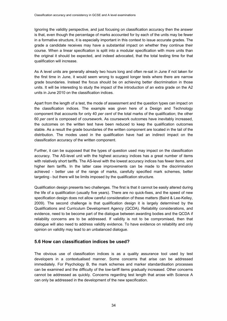
5.6 How can classification indices be used? The obvious use of classification indices is as a quality assurance tool used by test developers in a contextualised manner. Some concerns that arise can be addressed immediately. For Psychology B, the mark schemes and marker standardisation processes can be examined and the difficulty of the low-tariff items gradually increased. Other concerns cannot be addressed as quickly. Concerns regarding test length that arose with Science A can only be addressed in the development of the new specification.
34

Classification accuracy and consistency in GCSE and A level examinations
The monitoring and publishing of the values may be problematic on a routine basis as a high value of classification accuracy does not necessarily mean a high quality test. One of the Science A units suddenly increased in accuracy in June 2009. The test quality had not miraculously improved; a much more able cohort was taking it. The indices in themselves therefore may say more about the candidates than about the quality of the test. If classification indices are to be published then there is a choice to be made regarding which index. The Livingston and Lewis indices are lower than the IRT indices – and there are other procedures. Classification consistency is lower than classification accuracy. The focus on the middle grades is less population dependent, but a more conservative figure. The choice of index to publish could have important ramifications.
5.7 Are there any dangers with pursuing high classification indices? As long as the classification indices are not used in isolation there is little danger in trying to improve them as long as it is done within the constraints of validity. Unlike approaches built on Cronbach’s alpha the IRT approach assumes and imposes a single latent trait so there is no danger that the focus of the examinations will be narrowed to meet targets. It may be considered, however, that replacing longer items with poor discrimination with shorter items with better discrimination may improve the classification accuracy. In this case the construct under examination may change and the validity of the test would be under threat. It is worth re-emphasising the words of the 1975 report, therefore, that ‘striving to achieve reliability as an independent goal is simply a misdirection of effort.’ (Wilmott & Nuttall, 1975, p. 55)
5.8 Further research The key issue which undermines the currency of classification accuracy and consistency statistics is the dimensionality of the tests. For this reason it may be worth investigating multi-dimensional IRT models. The overall accuracy and consistency of grading once units have been aggregated would also be of interest. For completeness, once the first new A2 units have been sat in June 2010 it would be worth calculating classification indices for them.
5.9 Recommendations Interpretation of classification indices requires an understanding of the context of each assessment. The figures alone are not meaningful in themselves. For this reason it is suggested that case studies of certain units could be shared between those with the expertise to interpret them so that a shared understanding may develop. These groups may include Ofqual, other awarding bodies or a group of assessment experts. This process would promote understanding of how indices are likely to vary between awarding bodies, between specification designs and subjects, and over time. Until those directly involved in the qualifications have gained experience and understanding in the relevant indices it makes little sense to publish them. Until we fully understand them ourselves it would seem dangerous to release them to an unprepared public.
35

Classification accuracy and consistency in GCSE and A level examinations
If meaningful comparisons are to be made then consistency of choice of model and index matters. Using the same measures over time and between awarding bodies is essential if useful comparisons are to be made. First published by The Office of the Qualifications and Examinations Regulator in (2010). © Qualifications and Curriculum Authority (2010) Ofqual is part of the Qualifications and Curriculum Authority (QCA). QCA is an exempt charity under Schedule 2 of the Charities Act 1993.
36

Classification accuracy and consistency in GCSE and A level examinations
References
Baird, J., & Lee-Kelley, L. (2009). The dearth of managerialism in implementation of national examinations policy. Journal of Education Policy, 24(1), 55.
Breyer, F., & Lewis, C. (1994). Pass-fail reliability for tests with cut scores: A simplified method (ETS Research Report No. 94-39). Princeton, NJ: Educational Testing Service.
Cohen, J. (1960). A coefficient of agreement for nominal scales. Educational and Psychological Measurement, 20, 37-46.
Cresswell, M. (1984). A-Level Grades - How Many Should There Be? Guildford: Assessment and Qualifications Alliance.
Ebel, R. (1965). Measuring Educational Achievement. Englewood Cliffs, N.J.: Prentice-Hall. Green, S. B., (2009) Commentary on coefficient alpha: a cautionary tale. Psychometrika, 74,
121-135. Hanson, B. A., & Brennan, R. L. (1990). An investigation of classification consistency indexes
estimated under alternative strong true score models. Journal of Educational Measurement, 27, 345-359.
Hitchcock, C., & Sober, E. (2004). Prediction vs accommodation and the risk of overfitting. The British Journal for the Philosophy of Science, 55(1), 1-34.
Huynh, H. (1990). Computation and statistical inference for decision consistency indexes based on the Rasch model. Journal of Educational Statistics, 15, 353-368.
Huynh, H. (1976). On the reliability of decisions in domain-referenced testing. Journal of Educational Measurement, 13, 253-264.
Knupp, T., Lee, W., & Ansley, T. (2009). A method for estimating decision consistency using composite scores in an IRT framework. Presented at the Annual Meeting of the National Council on Measurement in Education, San Diego.
Kolen, M. J., & Brennan, R. L. (2004). Test Equating, Scaling, and Linking. Statistics in social science and public policy. New York: Springer.
Lee, W. (2008). Classification consistency and accuracy for complex assessments using item response theory (No. 27). CASMA Research Report. Iowa City, IA: Center for Advanced Studies in Measurement and Assessment, University of Iowa.
Lee, W. (2009). Current development and issues in estimating classification consistency and accuracy. Presented at the the Annual Meeting of the National Council on Measurement in Education, San Diego, CA.
Lee, W., Brennan, R. L., & Wan, L. (2009). Classification consistency and accuracy for complex assessments under the compound multinomial model. Applied Psychological Measurement, 33, 374-390.
Lee, W., Hanson, B. A., & Brennan, R. L. (2002). Estimating Consistency and Accuracy Indices for Multiple Classifications. Applied Psychological Measurement, 26(4), 412-432. doi: 10.1177/014662102237797
Lee, W., Wang, T., Kim, S., & Brennan, R. L. (2006). A strong true-score model for polytomous items (No. 16). CASMA Research Report. Iowa City, IA: Center for Advanced Studies in Measurement and Assessment, University of Iowa.
Livingston, S. A., & Lewis, C. (1995). Estimating the Consistency and Accuracy of Classifications Based on Test Scores. Journal of Educational Measurement, 32(2), 179-197.
Mair, P., & Hatzinger, R. (n.d.). eRm. Retrieved from http://cran.r-project.org/web/packages/eRm/eRm.pdf
Maris, G., & Bechger, T. (2006). Scoring open ended questions. In Handbook of Statistics, 26. Amsterdam, Netherlands: North-Holland.
37

Classification accuracy and consistency in GCSE and A level examinations
38
Mitchelmore, M. (1981). Reporting Student Achievement: How many Grades? British Journal of Educational Psychology, 51(2), 218-227.
Peng, C., & Subkoviak, M. J. (1980). A note on Huynh’s normal approximation procedure for estimating criterion-referenced reliability. Journal of Educational Measurement, 17, 359-368.
Pilliner, A. (1969). Estimation of number of grades to be awarded in an examination by consideration of its reliability coefficient. Edinburgh: The Godfrey Thomson Unit for Educational Research.
Please, N. (1971). Estimation of the proportion of candidates who are wrongly graded. British Journal of Mathematical and Statistical Psychology, 4(4), 447-467.
R Development Core Team. (n.d.). R: A Language and Environment for Statistical Computing. Vienna, Austria: R Foundation for Statistical Computing. Retrieved from http://www.R-project.org
Revelle, W. (2009a). psych: Procedures for Psychological, Psychometric, and Personality Research. Retrieved from http://CRAN.R-project.org/package=psych
Revelle, W. (2009b). Coefficients alpha, beta, omega, and the glb: comments on Sijtsma. Psychometrika, 74, 145-154.
Revelle, W. (1979). Hierarchical Cluster Analysis and the Internal Structure of Tests. Multivariate Behavioral Research, 14, 57-74.
Schulz, E., Kolen, M. J., & Nicewander, W. (1999). A rationale for defining achievement levels using IRT-estimated domain scores. Applied Psychological Measurement, 23, 347-362.
Sijtsma, K. (2009). On the use, the misuse, and the very limited usefulness of Cronbach's alpha. Psychometrika, 74, 107-120.
Subkoviak, M. J. (1976). Estimating reliability from a single administration of a criterion referenced test. Journal of Educational Measurement, 13, 265-276.
Wang, T., Kolen, M. J., & Harris, D. (2000). Psychometric properties of scale scores and performance levels for performance assessments using polytomous IRT. Journal of Educational Measurement, 37, 141-162.
Ward, J. (1972). The measuremeter: a useful psychometric concept. Associationof Educational Pyschologists' Journal and Newsletter, 3(2), 52-53.
Wiliam, D. (2009). The reliability of educational assessments. Annual Ofqual Lecture. Retrieved from http://www.dylanwiliam.net/
Wilmott, A., & Nuttall, D. (1975). Reliability of examinations at 16+. Schools Council Research Studies. London: Macmillan Education.
Woodruff, D. J., & Sawyer, R. L. (1989). Estimating measures of pass-fail reliability from parallel half-tests. Applied Psychological Measurement, 13, 33-43.
Zinbarg, R. E., Revelle, W., Yovel, I., & Li, W. (2005). Cronbach’s α, Revelle's β, and McDonald’S ωH : their relations with each other and two alternative conceptualizations of reliability. Psychometrika, 7(1), 123-133.
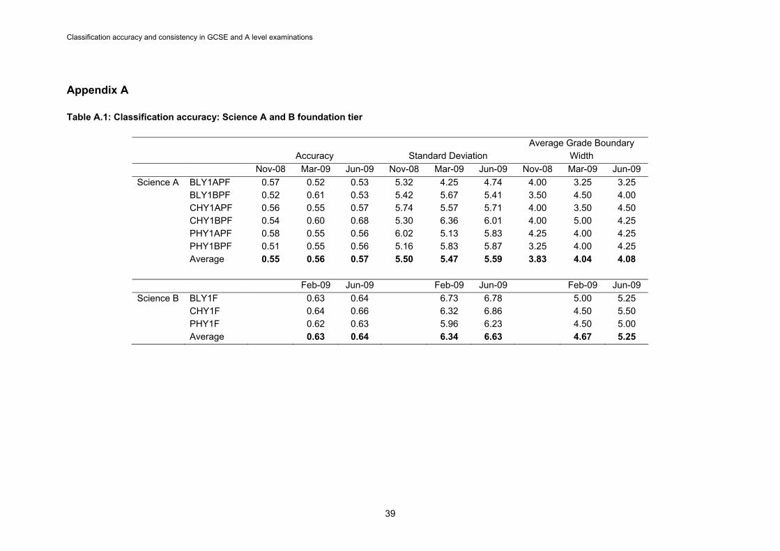
Classification accuracy and consistency in GCSE and A level examinations
Appendix A Table A.1: Classification accuracy: Science A and B foundation tier
Accuracy Standard Deviation Average Grade Boundary
Width
Nov-08 Mar-09 Jun-09 Nov-08 Mar-09 Jun-09 Nov-08 Mar-09 Jun-09
Science A BLY1APF 0.57 0.52 0.53 5.32 4.25 4.74 4.00 3.25 3.25 BLY1BPF 0.52 0.61 0.53 5.42 5.67 5.41 3.50 4.50 4.00 CHY1APF 0.56 0.55 0.57 5.74 5.57 5.71 4.00 3.50 4.50 CHY1BPF 0.54 0.60 0.68 5.30 6.36 6.01 4.00 5.00 4.25 PHY1APF 0.58 0.55 0.56 6.02 5.13 5.83 4.25 4.00 4.25 PHY1BPF 0.51 0.55 0.56 5.16 5.83 5.87 3.25 4.00 4.25
Average 0.55 0.56 0.57 5.50 5.47 5.59 3.83 4.04 4.08
Feb-09 Jun-09 Feb-09 Jun-09 Feb-09 Jun-09
Science B BLY1F 0.63 0.64 6.73 6.78 5.00 5.25 CHY1F 0.64 0.66 6.32 6.86 4.50 5.50 PHY1F 0.62 0.63 5.96 6.23 4.50 5.00 Average 0.63 0.64 6.34 6.63 4.67 5.25
39
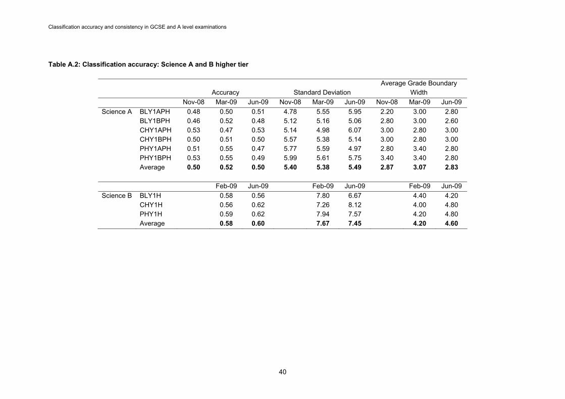
Classification accuracy and consistency in GCSE and A level examinations
Table A.2: Classification accuracy: Science A and B higher tier
Accuracy Standard Deviation Average Grade Boundary
Width
Nov-08 Mar-09 Jun-09 Nov-08 Mar-09 Jun-09 Nov-08 Mar-09 Jun-09
Science A BLY1APH 0.48 0.50 0.51 4.78 5.55 5.95 2.20 3.00 2.80 BLY1BPH 0.46 0.52 0.48 5.12 5.16 5.06 2.80 3.00 2.60 CHY1APH 0.53 0.47 0.53 5.14 4.98 6.07 3.00 2.80 3.00 CHY1BPH 0.50 0.51 0.50 5.57 5.38 5.14 3.00 2.80 3.00 PHY1APH 0.51 0.55 0.47 5.77 5.59 4.97 2.80 3.40 2.80 PHY1BPH 0.53 0.55 0.49 5.99 5.61 5.75 3.40 3.40 2.80
Average 0.50 0.52 0.50 5.40 5.38 5.49 2.87 3.07 2.83
Feb-09 Jun-09 Feb-09 Jun-09 Feb-09 Jun-09
Science B BLY1H 0.58 0.56 7.80 6.67 4.40 4.20 CHY1H 0.56 0.62 7.26 8.12 4.00 4.80 PHY1H 0.59 0.62 7.94 7.57 4.20 4.80
Average 0.58 0.60 7.67 7.45 4.20 4.60
40

Classification accuracy and consistency in GCSE and A level examinations
Table A.3 Classification accuracy: GCSE Maths foundation tier
Accuracy Standard DeviationAverage Grade Boundary Width
Nov-08 Jun-09 Nov-08 Jun-09 Nov-08 Jun-09
Maths A 4301/1F 0.75 0.77 16.88 18.20 12.00 13.25 4301/2F 0.74 0.78 16.47 18.88 11.50 14.25 Maths B 43051/F 0.63 0.68 7.37 8.49 4.50 6.25 43053/F 0.72 0.72 13.08 13.36 8.25 9.00 43055/1F 0.63 0.68 9.34 10.98 6.00 7.50 43055/2F 0.67 0.71 8.92 12.88 5.50 9.00
Table A.4 Classification accuracy: GCSE Maths higher tier
Accuracy Standard DeviationAverage Grade Boundary Width
Nov-08 Jun-09 Nov-08 Jun-09 Nov-08 Jun-09
Maths A 4301/1H 0.74 0.77 19.37 18.68 12.20 13.20 4301/2H 0.73 0.76 20.43 19.02 12.20 13.60 Maths B 43051/H 0.62 0.65 8.21 8.80 6.40 6.60 43053/H 0.64 0.67 13.71 14.51 7.60 9.20 43055/1H 0.59 0.68 11.54 12.30 5.40 8.40 43055/2H 0.64 0.67 15.82 13.32 8.00 8.80
41

Classification accuracy and consistency in GCSE and A level examinations
42
Table A.5 Classification accuracy: Miscellaneous linear foundation tier GCSE June 2009
Specification Component AccuracyStandard Deviation
Average Grade
Boundary Width
Geography B 3032/1F 0.58 9.68 5.00
Geography B 3032/2F 0.64 14.49 9.50
Business and Communication Systems 3126/1F 0.62 9.63 6.00
Statistics 3311/F 0.78 14.31 8.25
ICT A 3521/F 0.63 10.06 2.50
Design & Technology (Electronic Products) 3541/F 0.73 18.16 6.00
Table A.6 Classification accuracy: Miscellaneous linear higher tier GCSE June 2009
Specification Component AccuracyStandard Deviation
Average Grade
Boundary Width
Geography B 3032/1H 0.60 10.49 5.80
Geography B 3032/2H 0.61 17.32 9.20
Business and Communication Systems 3126/1H 0.69 8.75 9.40
Statistics 3311/H 0.71 17.31 11.80
ICT A 3521/H 0.51 8.08 4.40
Design & Technology (Electronic Products) 3541/H 0.62 18.62 9.60

Classification accuracy and consistency in GCSE and A level examinations
Appendix B A number of different coefficients are available to estimate the reliability of assessments and much recent discussion has surrounded their appropriateness (Sijtsma, 2009; Revelle, 2009b; Green, 2009; Zinbarg, Revelle, Yovel, & Li, 2005). Due to clear practical issues with multiple administrations of assessments, these discussions are largely concerned with estimation of reliability based on a single administration. The most widely reported reliability coefficient, Cronbach’s alpha, has been subject to examination regarding its accuracy in estimating the reliability under the practical conditions associated with the single administration approach where it can be shown to underestimate the reliability (Revelle, 2009b; Sijtsma, 2009). The shortcomings of such a measure are conceded in this study however the values of alpha are reported below for comparison with other work. As alpha can provide values lower than common alternatives, the consequence of its use as a measure of reliability for incorporation into the Livingston-Lewis procedure is to reduce the equivalent dichotomous test length. Therefore, for the non-IRT approach implemented here, the use of alternative reliability coefficients would raise the measures of classification consistency and accuracy from the lower limits reported. Table B.1: Alpha coefficients for the considered AS level units
Specification Unit Alpha
ACCOUNTING ACCN1 0.76
ACCOUNTING ACCN2 0.78
BIOLOGY BIOL1 0.85
BIOLOGY BIOL2 0.89
CHEMISTRY CHEM1 0.91
CHEMISTRY CHEM2 0.94
COMPUTING COMP2 0.84
ELECTRONICS ELEC1 0.90
ELECTRONICS ELEC2 0.93
ENVIRONMENTAL STUDIES ENVS1 0.77
ENVIRONMENTAL STUDIES ENVS2 0.88
HUMAN BIOLOGY HBIO1 0.87
HUMAN BIOLOGY HBIO2 0.84
PHYSICS PHYA1 0.91
PHYSICS A PHYA2 0.92
PHYSICS B PHYB2 0.90
PSYCHOLOGY A PSYA1 0.83
PSYCHOLOGY A PSYA2 0.84
PSYCHOLOGY B PSYB1 0.77
SCIENCE IN SOCIETY SCIS1 0.85
43

We wish to make our publications widely accessible. Please contact us if you have any specific accessibility requirements.
First published by the Office of Qualifications and Examinations Regulation in 2011
© Crown copyright 2011
Office of Qualifications and Examinations Regulation Spring Place 2nd Floor Coventry Business Park Glendinning House Herald Avenue 6 Murray Street Coventry CV5 6UB Belfast BT1 6DN
Telephone 0300 303 3344 Textphone 0300 303 3345 Helpline 0300 303 3346
www.ofqual.gov.uk