Classical Prandtl-Ishlinskii modeling and inverse multiplicativestructure to compensate hysteresis in piezoactuators

Micky Rakotondrabe, Member, IEEE

Abstract— This paper presents a new approach tocompensate the static hysteresis in smart materialbased actuators that is modeled by the Prandtl-Ishlinskii approach. The proposed approach allows asimplicity and ease of implementation. Furthermore,as soon as the direct model is identified and obtained,the compensator is directly derived. The experimentalresults on piezoactuators show its efficiency and proveits interest for the precise control of microactuatorswithout the use of sensors. In particular, we exper-imentally show that the hysteresis of the studiedactuator which was initially 23% was reduced to lessthan 2.5% for the considered working frequency.

I. Introduction

Piezoelectric ceramics (piezoceramics) are very prizedin the design of microrobots, micro/nanopositioning de-vices and systems at the micro/nano scale in general.They have been successfully used to develop steppermicrorobots [1][2], Atomic Force Microscopes (AFM) [3]and continuous microactuators such as piezocantileversand microgrippers [4][5]. This recognition is mainlythanks to the high resolution (at the nanometre level),the high bandwidth (more than 1kHz) and the relativelyhigh force density that they offer. However, when theapplied electrical field is large, piezoceramics exhibit animportant hysteresis nonlinearity which strongly limitsthe accuracy of the developed actuators.

Three approaches exist to control the hysteresis and toimprove the general performance of piezoelectric actua-tors (piezoactuators): feedback control, charge control,and feedforward voltage control. In feedback control,both classical (PID, ...) and advanced control laws (H∞,passivity,...) have been successfully used [6][7]. Its mainadvantages are the possibility to reject external distur-bance effects and to account for the model uncertainties.However, the use of closed loop control techniques atthe micro/nano scale is strongly limited by the difficultyto integrate sensors. Sensors which are precise and fastenough are bulky (interferometers, triangulation opticalsensors, camera-microscopes measurement systems, etc.)or difficult to fabricate. In charge control, an adaptedelectrical circuit is used to provide the input chargeapplied to the piezoactuators [8][9][10]. Finally, in feed-forward voltage control, the hysteresis is precisely mod-

FEMTO-st Institute,UMR CNRS-6174 / UFC / ENSMM / UTBMAutomatic Control and Micro-Mechatronic Systems department

(AS2M department)25000 Besancon - Francemrakoton@femto-st.fr

eled and a kind of inverse model is put in cascade withthe process resulting in an overall linearized system.The main advantage of the two latter approaches isthe shunning of external sensors making the controlledsystem packageable and fabricated with low cost. In anautomatic point of view, feedforward voltage control isparticularly appreciated because this approach allowsstability, performance analysis and controllers synthesis.

For piezoactuators, there exist several approaches ofhysteresis compensation based on voltage control: theBouc-Wen [11], the polynomial [12], the lookup tables[13], the Preisach [14][15] and the classical Prandtl-Ishlinskii approaches [16][17][18]. The Prandtl-Ishlinskiiapproach is particularly appreciated for its simplicity,ease of implementation and accuracy. It is based on thesum of many elementary hysteresis backlash operators.The accuracy of the model increases with the number ofthese operators. To compute the corresponding hysteresiscompensator, the least-squared error optimization hasbeen used [17]. However the computation time greatlyincreases according to the number of operators whichmakes this method only practical for low number ofbacklash operators. In this paper, we propose anothercompensation approach for hysteresis modelled by thePrandtl-Ishlinskii. Based on the inverse multiplicativestructure, the proposed approach does not need anycomputation of the compensator. Indeed, as soon as themodel is identified, the compensator is derived withoutextra-calculation. Therefore, independant from the num-ber of the backlashes (and whatever the required accu-racy), there is no cost for the compensator computation.

II. The classical Prandtl-Ishlinskii modelingand identification

The classical Prandtl-Ishlinskii (PI) model is based onthe backlash operator.

A. The backlash operator

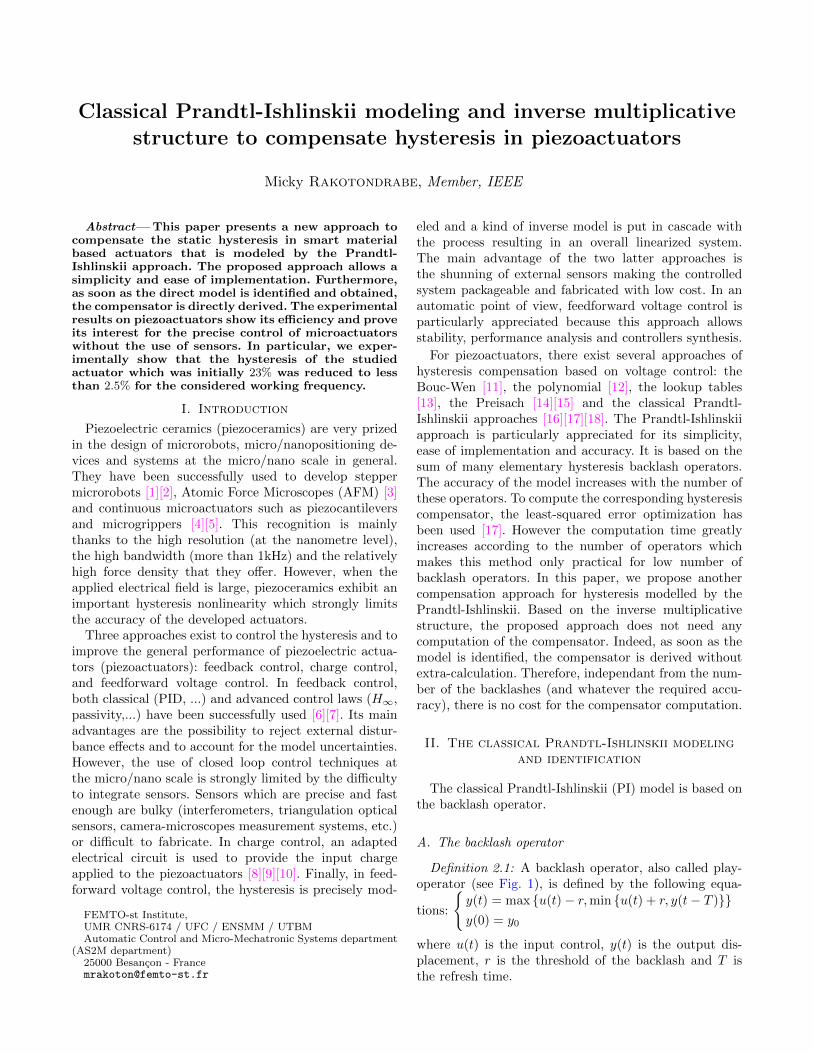
Definition 2.1: A backlash operator, also called play-operator (see Fig. 1), is defined by the following equa-

tions:

{y(t) = max {u(t)− r,min {u(t) + r, y(t− T )}}y(0) = y0

where u(t) is the input control, y(t) is the output dis-placement, r is the threshold of the backlash and T isthe refresh time.

( )u t

( )y t

r-r

Fig. 1. A backlash operator with a slope unity.

B. The classical PI model

Definition 2.2: A classical PI hysteresis model isdefined as the sum of several backlashes each one havinga threshold ri and a slope (weighting) wi [19]: y(t) =

n∑i=1

wi ·max {u(t)− ri,min {u(t) + ri, yei(t− T )}}

y(0) = y0

where n is the number of operators and yei the ith

elementary output (output of the ith backlash). Fig. 2gives the block diagram showing the principle of theclassical PI hysteresis modeling.

1w

2w

nw

∑

backlash

weighting

( )y t( )u t

. . .

Fig. 2. Diagram showing the principle of the classical PI modeling.

C. Parameters identification

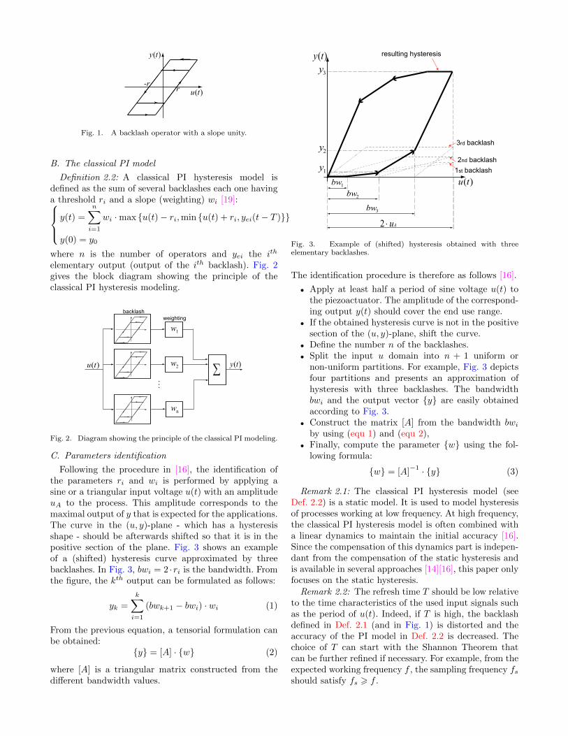
Following the procedure in [16], the identification ofthe parameters ri and wi is performed by applying asine or a triangular input voltage u(t) with an amplitudeuA to the process. This amplitude corresponds to themaximal output of y that is expected for the applications.The curve in the (u, y)-plane - which has a hysteresisshape - should be afterwards shifted so that it is in thepositive section of the plane. Fig. 3 shows an exampleof a (shifted) hysteresis curve approximated by threebacklashes. In Fig. 3, bwi = 2 ·ri is the bandwidth. Fromthe figure, the kth output can be formulated as follows:

yk =

k∑i=1

(bwk+1 − bwi) · wi (1)

From the previous equation, a tensorial formulation canbe obtained:

{y} = [A] · {w} (2)

where [A] is a triangular matrix constructed from thedifferent bandwidth values.

1bw

2bw

3bw

2 uA⋅

( )y t

( )u t

1y

2y

3y

1st backlash

2nd backlash

3rd backlash

resulting hysteresis

Fig. 3. Example of (shifted) hysteresis obtained with threeelementary backlashes.

The identification procedure is therefore as follows [16].

• Apply at least half a period of sine voltage u(t) tothe piezoactuator. The amplitude of the correspond-ing output y(t) should cover the end use range.

• If the obtained hysteresis curve is not in the positivesection of the (u, y)-plane, shift the curve.

• Define the number n of the backlashes.• Split the input u domain into n + 1 uniform or

non-uniform partitions. For example, Fig. 3 depictsfour partitions and presents an approximation ofhysteresis with three backlashes. The bandwidthbwi and the output vector {y} are easily obtainedaccording to Fig. 3.

• Construct the matrix [A] from the bandwidth bwiby using (equ 1) and (equ 2),

• Finally, compute the parameter {w} using the fol-lowing formula:

{w} = [A]−1 · {y} (3)

Remark 2.1: The classical PI hysteresis model (seeDef. 2.2) is a static model. It is used to model hysteresisof processes working at low frequency. At high frequency,the classical PI hysteresis model is often combined witha linear dynamics to maintain the initial accuracy [16].Since the compensation of this dynamics part is indepen-dant from the compensation of the static hysteresis andis available in several approaches [14][16], this paper onlyfocuses on the static hysteresis.

Remark 2.2: The refresh time T should be low relativeto the time characteristics of the used input signals suchas the period of u(t). Indeed, if T is high, the backlashdefined in Def. 2.1 (and in Fig. 1) is distorted and theaccuracy of the PI model in Def. 2.2 is decreased. Thechoice of T can start with the Shannon Theorem thatcan be further refined if necessary. For example, from theexpected working frequency f , the sampling frequency fsshould satisfy fs > f .

III. A new compensation approach for the PIhysteresis modeling

In this section, we propose a new compensationmethod for the classical PI hysteresis model previouslypresented. The advantage of the proposed method is thatas soon as the model is identified, the compensator isdirectly derived without additional calculation. For that,we need to rewrite the PI model.

A. General principle

Definition 3.1: The (feedforward) compensation ofpiezoelectric materials hysteresis consists in putting incascade with the hysteretic system a compensator (seeFig. 4) such that one obtains a linear input-ouptut(yr, y) with a unity gain between the reference input yrand the output y [20]: ∂y

∂yr= 1

Remark 3.1: expression ∂y∂yr

= 1 in Def. 3.1 is similarto y = yr.

( )y t( )u t( )ry t

process

(modelled with a PI model)

compensator

(another PI model)

Fig. 4. Compensation of a hysteresis.

B. Rewriting the model

First we shall rewrite the hysteresis model alreadydefined in Def. 2.2. For that, we need to give a propertyof the backlash operator.

Property 3.1: Reconsider the backlash operator inDef. 2.1. We have: r = 0 ⇔ y(t) = u(t)So we have the following consequence which is an alter-native expression of Def. 2.2.

Consequence 3.1: A classical PI hystere-sis model can be expressed as follows:

y(t) = −u(t)

+

n∑i=0

wi ·max {u(t)− ri,min {u(t) + ri, yei(t− T )}}

y(0) = y0where ri and wi (for i = 1 · · ·n) are known according tothe above identification procedure. For i = 0, we have:r0 = 0 and w0 = 1.Proof: We rewrite the first equation in Def. 2.2 as follows:y(t) = u(t)− u(t)

+

n∑i=1

wi ·max {u(t)− ri,min {u(t) + ri, yei(t− T )}}

According to Property 3.1, u(t) can be expressed usingthe backlash operator by using a threshold r0 = 0.Multiplying the result by a weighting w0 = 1, we obtain:u(t) = w0 · max {u(t)− r0,min {u(t) + r0, ye0(t− T )}}Using the two previous equations, we deriveConsequence. 3.1.

C. A new compensator for the hysteresis

First, we give a consequence of Remark 2.1 and Re-mark 2.2 that will be used further.

Consequence 3.2: Define a compensator with inputyr(t) and output u(t). From Remark 2.1 (du(t)dt islow) and Remark 2.2 (T is very low), we have:∣∣∣ ∂u(t)∂yr(t)

− ∂u(t−T )∂yr(t)

∣∣∣ → 0 where ∂u(t)∂yr(t)

is the slope of the

compensator map (yr(t), u(t)).

Proof: Since du(t)dt and T are both low, we have

du(t−T )dt also low. Thus, we derive

∣∣∣du(t)dt −du(t−T )

dt

∣∣∣ →0 The latter expression can be rewritten as fol-

lows:∣∣∣ ∂u(t)∂yr(t)

.dyr(t)dt −∂u(t−T )∂yr

.dyr(t)dt

∣∣∣ → 0 which yields:∣∣∣ ∂u(t)∂yr(t)− ∂u(t−T )

∂yr

∣∣∣ . ∣∣∣dyr(t)dt

∣∣∣ → 0 For any continuous

and differentiable yr(t) and for any∣∣∣dyr(t)dt

∣∣∣, the pre-

vious expression is obtained iif:∣∣∣ ∂u(t)∂yr(t)

− ∂u(t−T )∂yr

∣∣∣ →0 To sum up, if du(t)

dt and T are both low, we have∣∣∣ ∂u(t)∂yr(t)− ∂u(t−T )

∂yr

∣∣∣→ 0.

Let us now give the new compensator.

Theorem 3.1: Reconsider the PI hysteresismodel in Def. 2.2 which is rewritable as inCons. 3.1. If the compensator is defined by:

u(t) =n∑i=0

wi ·max

{u(t− T )− ri,min {u(t− T ) + ri, yei(t− 2T )}

}−yr(t)

then ∂y∂yr

' 1 and therefore, the hysteresis iscompensated.

Proof: Replacing u(t) of the model inConsequence. 3.1 by the proposed compensatorin Theo. 3.1, we obtain: y(t) = yr(t) + O whereO = u(t)− u(t− T )

+

n∑i=1

wi ·max {u(t)− ri,min {u(t) + ri, yei(t− T )}}

−n∑i=1

wi ·max

{u(t− T )− ri,min

{u(t− T ) + ri,

yei(t− 2T )

}}Knowing that the model is independant from the

reference, i.e.:∂

n∑i=1

wi·max{u(t)−ri,min{u(t)+ri,yei(t−T )}}

∂yr=

0 we derive: ∂O∂yr

= ∂u(t)∂yr(t)

− ∂u(t−T )∂yr(t)

which - according to

Consequence. 3.2 - means ∂O∂yr→ 0 Finally, we deduce

that: ∂y(t)∂yr

= ∂yr∂yr

+ ∂O∂yr' 1

We have demonstrated that using the compensator givenin Theo. 3.1, the hysteresis modelled by a classical PItechnique was compensated. It is reminded that theproposed compensator contains the initial model itself(up to a signal −u(t) and up to period T ) according toCons. 3.1. This means that there is no extra-calculationof the compensator since it uses the same parameters andstructures than the initial model.

D. Parameters and implementation of the proposed com-pensator

The proposed compensator is identified and imple-mented as follows.

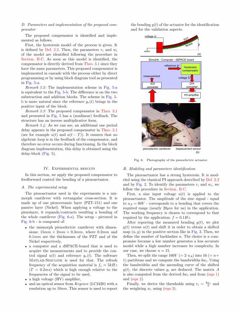
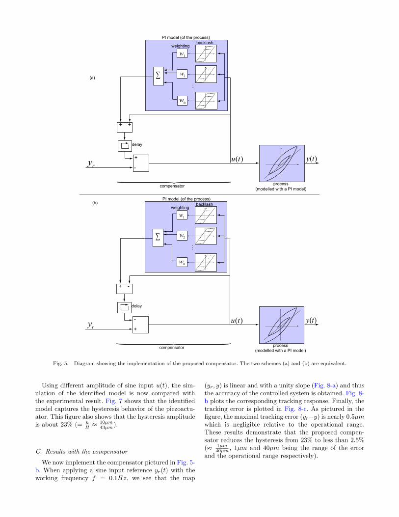
First, the hysteresis model of the process is given. Itis defined by Def. 2.2. Then, the parameters ri and wiof the model are identified following the procedure inSection. II-C. As soon as this model is identified, thecompensator is directly derived from Theo. 3.1 since theyhave the same parameters. This proposed compensator isimplemented in cascade with the process either by directprogramming or by using block diagram tool as presentedin Fig. 5-a.

Remark 3.2: The implementation scheme in Fig. 5-ais equivalent to the Fig. 5-b. The difference is on the twosubstraction and addition blocks. The scheme in Fig. 5-b is more natural since the reference yr(t) brings in thepositive input of the block.

Remark 3.3: The proposed compensator in Theo. 3.1and presented in Fig. 5 has a (nonlinear) feedback. Thestructure has an inverse multiplicative form.

Remark 3.4: As we can see, an additional one perioddelay appears in the proposed compensator in Theo. 3.1(see for example u(t) and u(t − T )). It ensures that noalgebraic loop is in the feedback of the compensator, andtherefore no error occurs during functioning. In the blockdiagram implementation, this delay is obtained using thedelay-block (Fig. 5).

IV. Experimental results

In this section, we apply the proposed compensator tofeedforward control the bending of a piezoactuator.

A. The experimental setup

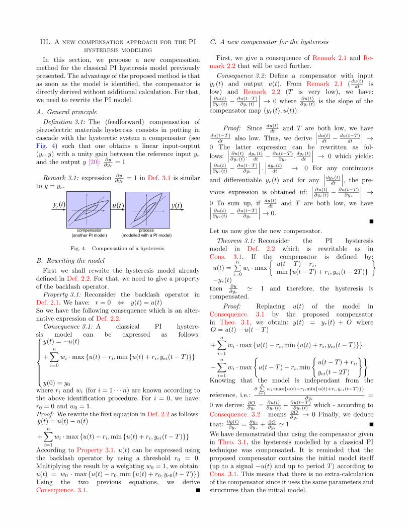
The piezoactuator used in the experiments is a uni-morph cantilever with rectangular cross-section. It ismade up of one piezoceramic layer (PZT-151) and onepassive layer (Nickel). When applying a voltage to thepiezolayer, it expands/contracts resulting a bending ofthe whole cantilever (Fig. 6-a). The setup - pictured inFig. 6-b - is composed of:

• the unimorph piezoelectric cantilever with dimen-sions: 15mm × 2mm × 0.3mm, where 0.2mm and0.1mm are the thicknesses of the PZT and of theNickel respectively,

• a computer and a dSPACE-board that is used toacquire the measurements and to provide the con-trol signal u(t) and reference yr(t). The softwareMatlab-Simulink is used for that. The refreshfrequency of the acquisition material is fs = 5kHz(T = 0.2ms) which is high enough relative to thefrequencies of the signal to be used,

• a high voltage (HV) amplifier,• and an optical sensor from Keyence (LC2420) with a

resolution up to 10nm. This sensor is used to report

the bending y(t) of the actuator for the identificationand for the validation aspects.

piezoelectric cantilever

Simulink - Computer - dSPACE board

(a)

(b)

PZT

Nickel

measurement

displacement sensor

10mm

HV-amplifier

D/A

converterA/D

converter

Hysteresis

compensator

reference yr

y

voltage U

voltage u

Fig. 6. Photography of the piezoelectric actuator.

B. Modeling and parameters identification

The piezoactuator has a strong hysteresis. It is mod-eled using the classical PI approach described by Def. 2.2and by Fig. 2. To identify the parameters ri and wi, wefollow the procedure in Section. II-C.

First, a sine input voltage u(t) is applied to thepiezoactuator. The amplitude of the sine signal - equalto uA = 80V - corresponds to a bending that covers therequired range (nearly 20µm for us) in the application.The working frequency is chosen to correspond to thatrequired by the application: f = 0.1Hz.

After reporting the measured bending y(t), we ploty(t) versus u(t) and shift it in order to obtain a shiftedmap (u, y) in the positive section like in Fig. 3. Then, wedefine the number of backlashes n. The choice is a com-promise because a low number generates a less accuratemodel while a high number increases its complexity. Inour case, we choose n = 15.

Then, we split the range 160V (= 2·uA) into 16 (= n+1) partitions and we compute the bandwidths bwi. Usingthe bandwidths and the ascending curve of the shiftedy(t), the discrete values yi are deduced. The matrix Ais also computed from the derived bwi and from (equ 1)and (equ 2).

Finally, we derive the thresholds using ri = bwi

2 andthe weighting wi using (equ 3).

( )y t( )u t

process

(modelled with a PI model)compensator

delay

PI model (of the process)

PI model (of the process)

1w

2w

nw

∑

backlashweighting

. . .

-

+ +

+

ry

( )y t( )u t

process

(modelled with a PI model)compensator

delay

1w

2w

nw

∑

backlashweighting

. . .

+

+ -

-

ry

(a)

(b)

Fig. 5. Diagram showing the implementation of the proposed compensator. The two schemes (a) and (b) are equivalent.

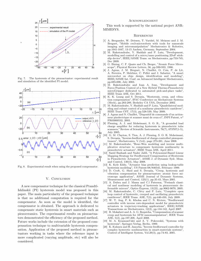
Using different amplitude of sine input u(t), the sim-ulation of the identified model is now compared withthe experimental result. Fig. 7 shows that the identifiedmodel captures the hysteresis behavior of the piezoactu-ator. This figure also shows that the hysteresis amplitudeis about 23% (= h

H ≈10µm43µm ).

C. Results with the compensator

We now implement the compensator pictured in Fig. 5-b. When applying a sine input reference yr(t) with theworking frequency f = 0.1Hz, we see that the map

(yr, y) is linear and with a unity slope (Fig. 8-a) and thusthe accuracy of the controlled system is obtained. Fig. 8-b plots the corresponding tracking response. Finally, thetracking error is plotted in Fig. 8-c. As pictured in thefigure, the maximal tracking error (yr−y) is nearly 0.5µmwhich is negligible relative to the operational range.These results demonstrate that the proposed compen-sator reduces the hysteresis from 23% to less than 2.5%(≈ 1µm

40µm , 1µm and 40µm being the range of the errorand the operational range respectively).

−80 −60 −40 −20 0 20 40 60 80−25

−20

−15

−10

−5

0

5

10

15

20

25

: experimental result

: simulation of the PI model

[ ]y µm

[ ]u V

h

h

H

Fig. 7. The hysteresis of the piezoactuator: experimental resultand simulation of the identified PI model.

[ ]ry µm

[ ]t s

[ ]t s

−20 −15 −10 −5 0 5 10 15 20

−20

0

20

40

0 10 20 30 40 50 60

−20

0

20

0 10 20 30 40 50 60−1

−0.5

0

0.5

: output

: reference

( )y t( )ry t

(a)

(b)

(c)

[ ]y µm

( ) - y(t) [µm]ry terror

Fig. 8. Experimental result when using the proposed compensator.

V. Conclusion

A new compensator technique for the classical Prandtl-Ishlinskii (PI) hysteresis model was proposed in thispaper. The main particularity of the proposed techniqueis that no additional computation is required for thecompensator. As soon as the model is identified, thecompensator is obtained. The approach is dedicated tocompensate static hysteresis in smart materials such aspiezoceramics. The experimantal results on piezoactua-tors demonstrated the efficiency of the proposed method.Future works include the extension of the proposed com-pensation technique to multivariable hysteresis compen-sation. Application of the proposed method in piezoac-tuators working in tasks where the reference input ismore complicated (varying amplitude, etc) will also beconsidered.

Acknowledgment

This work is supported by the national project ANR-MIMESYS.

References

[1] A. Bergander, W. Driesen, T. Varidel, M. Meizoso and J. M.Breguet, ”Mobile cm3-microrobots with tools for nanoscaleimaging and micromanipulation” Mechatronics & Robotics,pp.1041-1047, 13-15 Aachen, Germany, September 2004.

[2] M. Rakotondrabe, Y. Haddab and P. Lutz, ”Development,modelling and control of a micro/nano positioning 2DoF stick-slip device”, IEEE/ASME Trans. on Mechatronics, pp:733-745,Dec 2009.

[3] G. Bining, C. F. Quate and Ch. Berger, ”Atomic Force Micro-scope”, Physical Review Letters, 56, pp.930-933, 1986.

[4] J. Agnus, J. M. Breguet, N. Chaillet, O. Cois, P. de Lit,A. Ferreira, P. Melchior, C. Pellet and J. Sabatier, ”A smartmicrorobot on chip: design, identification and modeling”,IEEE/ASME Int. Conf. on Advanced Intelligent Mechatronics,pp.685-690, July 2003.

[5] M. Rakotondrabe and Ioan A. Ivan, ”Development andForce/Position Control of a New Hybrid Thermo-PiezoelectricmicroGripper dedicated to automated pick-and-place tasks”,IEEE Trans ASE, Oct 2011.

[6] K. K. Leang and S. Devasia, ”Hysteresis, creep, and vibra-tion compensation”, IFAC Conference on Mechatronic Systems(Mech), pp.283-289, Berkeley CA USA, December 2002.

[7] M. Rakotondrabe, Y. Haddab and P. Lutz, ”Quadrilateral mod-eling and robust control of a nonlinear piezoelectric cantilever”,IEEE Trans CST, 17(3), pp.528-539, May 2009.

[8] J. Agnus and N. Chaillet, ”Dispositif de commande d’un action-neur pizolectrique et scanner muni de ceux-ci”, INPI Patent, no

FR03000532, 2003.[9] Fleming, A. J. and Moheimani, S. O. R., ”A grounded load

charge amplifier for reducing hysteresis in piezoelectric tubescanners,” Review of Scientific Instruments, 76(7), 073707(1-5),July 2005.

[10] G. M. Clayton, S. Tien, A. J. Fleming, S. O. R. Moheimani,S. Devasia, ”Inverse-feedforward of charge-controlled piezoposi-tioners”, Mechatronics, V.(5-6), page 273-281, June 2008.

[11] M. Rakotondrabe, ”Bouc-Wen modeling and inverse multi-plicative structure to compensate hysteresis nonlinearity inpiezoelectric actuators”, IEEE Trans ASE, April 2011.

[12] Saeid Bashash and Nader Jalili, ”A Polynomial-Based LinearMapping Strategy for Feedforward Compensation of Hysteresisin Piezoelectric Actuators”, ASME J. of Dynamic Syst. Meas.and Control, 130(3), May 2008.

[13] K. Kyle Eddy, ”Actuator bias prediction using lookup-tablehysteresis modeling”, US Patent-08/846545, February 1999.

[14] D. Croft, G. Shed and S. Devasia, ”Creep, hysteresis andvibration compensation for piezoactuators: atomic force mi-croscopy application”, ASME Journal of Dynamic Systems,Measurement and Control, 123(1), pp.35-43, Mars 2001.

[15] A. Dubra and J. Massa and C.l Paterson, ”Preisach classi-cal and nonlinear modeling of hysteresis in piezoceramic de-formable mirrors”, Optics Express, 13(22), pp.9062-9070, 2005.

[16] M. Rakotondrabe, C. Clevy and P. Lutz, ”Complete openloop control of hysteretic, creeped and oscillating piezoelectriccantilevers”, IEEE Trans. ASE, 7(3), pp:440-450, July 2009.

[17] W. T. Ang, P. K. Kholsa and C. N. Riviere, ”Feedforwardcontroller with inverse rate-dependent model for piezoelectricactuators in trajectory-tracking applications”, IEEE/ASMETransactions on Mechatronics, 12(2), pp.134-142, April 2007.

[18] B. Mokaberi and A. A. G. Requicha, ”Compensation of scannercreep and hysteresis for AFM nanomanipulation”, IEEE TransASE, 5(2), pp.197-208, April 2008.

[19] M. A. Krasnosel’skii and A. V. Pokrovskii, ”Systems withhysteresis”, Springer-Verlag, Berlin, 1989.

[20] K. Kuhnen and H. Janocha, ”Inverse feedforward controller forcomplex hysteretic nonlinearities in smart-materials systems”,Control of Intelligent System, Vol.29(3), pp.74-83, 2001.