Classical Optimization Theory:

Constrained Optimization

(Equality Constraints)

1

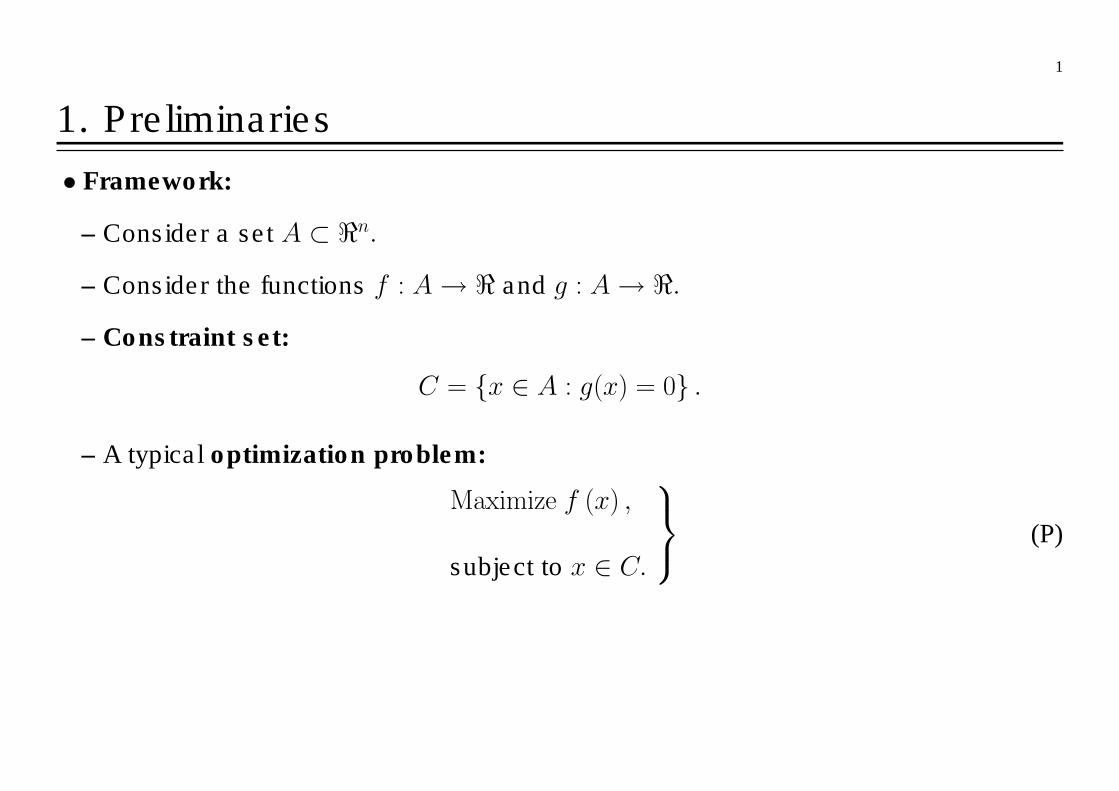
1. Preliminaries

• Framework:

– Consider a set A ⊂ <n.

– Consider the functions f : A→ < and g : A→ <.

– Constraint set:

C = {x ∈ A : g(x) = 0} .

– A typical optimization problem:

Maximize f (x) ,

subject to x ∈ C.

(P)

2

• Local Maximum:

A point x∗ ∈ C is said to be a point of local maximum of f subject to the constraints

g(x) = 0, if there exists an open ball around x∗, Bε (x∗) , such that f (x∗) ≥ f (x) for

all x ∈ Bε (x∗) ∩ C.

• Global Maximum:

A point x∗ ∈ C is a point of global maximum of f subject to the constraint g(x) = 0,if x∗ solves the problem (P).

• Local minimum and global minimum can be defined similarly by just reverting the

inequalities.

3

2. Necessary Conditions for Constrained Local Maximumand Minimum

• The basic necessary condition for a constrained local maximum is provided by La-

grange’s theorem.

• Theorem 1(a) (Lagrange Theorem: Single Equality Constraint):

Let A ⊂ <n be open, and f : A → <, g : A → < be continuously differentiable

functions on A. Suppose x∗ is a point of local maximum or minimum of f subject to

the constraint g(x) = 0. Suppose further that Og(x∗) 6= 0. Then there is λ∗ ∈ < such

that

Of (x∗) = λ∗ · Og(x∗). (1)

– The (n + 1) equations given by (1) and the constraint g(x) = 0 are called the first-

order conditions for a constrained local maximum or minimum.

4

• There is an easy way to remember the conclusion of Lagrange Theorem.

– Consider the function L : A×< → < defined by

L (x, λ) = f (x)− λg (x) .

– L is known as the Lagrangian, and λ as the Lagrange multiplier.

– Consider now the problem of finding the local maximum (or minimum) in an uncon-

strained maximization (or minimization) problem in which L is the function to be

maximized (or minimized).

– The first-order conditions are:

DiL (x, λ) = 0, for i = 1, ..., n + 1,

which yields

Dif (x) = λDig (x) , for i = 1, ..., n; and g(x) = 0.

– The first n equations can be written as Of (x) = λ · Og(x) as in the conclusion of

Lagrange Theorem.

– The method described above is known as the “Lagrange multiplier method”.

5

• The Constraint Qualification:

The condition, Og(x∗) 6= 0, is known as the constraint qualification.

– It is particularly important to check the constraint qualification before applying the

conclusion of Lagrange’s Theorem.

- Without this condition, the conclusion of Lagrange’s Theorem would not be valid,

as the following example shows.

#1. Let f : <2 → < be given by f (x1, x2) = 2x1 + 3x2 for all (x1, x2) ∈ <2, and

g : <2 → < be given by g (x1, x2) = x21 + x22 for all (x1, x2) ∈ <2.

– Consider the constraint set

C ={(x1, x2) ∈ <2 : g (x1, x2) = 0

}.

– Now consider the maximization problem: Maximize(x1,x2)∈C

f (x1, x2) .

(a) Demonstrate that the conclusion of Lagrange’s Theorem does not hold here.

(b) What is the solution to the maximization problem?

(c) What goes wrong? Explain clearly.

6

• Several Equality Constraints:

In Problem (P) we have considered only one equality constraint, g(x) = 0. Now we

consider more than one, saym, equality constraints: gj : A→ <, such that gj(x) = 0,j = 1, 2, ...,m.

– Constraint set:

C ={x ∈ A : gj(x) = 0, j = 1, 2, ...,m

}.

– Constraint Qualification:

The natural generalization of the constraint qualification with single constraint,

Og(x∗) 6= 0, involves the Jacobian derivative of the constraint functions:

Dg (x∗) =

∂g1

∂x1(x∗)

∂g1

∂x2(x∗) · · · ∂g1

∂xn(x∗)

∂g2

∂x1(x∗)

∂g2

∂x2(x∗) · · · ∂g2

∂xn(x∗)

... ... . . . ...∂gm

∂x1(x∗)

∂gm

∂x2(x∗) · · · ∂g

m

∂xn(x∗)

.

7

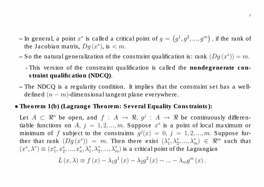
– In general, a point x∗ is called a critical point of g =(g1, g2, ..., gm

), if the rank of

the Jacobian matrix, Dg (x∗), is < m.

– So the natural generalization of the constraint qualification is: rank (Dg (x∗)) = m.

- This version of the constraint qualification is called the nondegenerate con-

straint qualification (NDCQ).

– The NDCQ is a regularity condition. It implies that the constraint set has a well-

defined (n−m)-dimensional tangent plane everywhere.

• Theorem 1(b) (Lagrange Theorem: Several Equality Constraints):

Let A ⊂ <n be open, and f : A → <, gj : A → < be continuously differen-

tiable functions on A, j = 1, 2, ...,m. Suppose x∗ is a point of local maximum or

minimum of f subject to the constraints gj(x) = 0, j = 1, 2, ...,m. Suppose fur-

ther that rank (Dg (x∗)) = m. Then there exist (λ∗1, λ∗2, ..., λ

∗m) ∈ <m such that

(x∗, λ∗) ≡ (x∗1, x∗2, ..., x∗n, λ∗1, λ∗2, ..., λ∗m) is a critical point of the Lagrangian

L (x, λ) ≡ f (x)− λ1g1 (x)− λ2g2 (x)− ...− λmgm (x) .

8

In other words,

∂L

∂xi(x∗, λ∗) = 0, i = 1, 2, ..., n,

and (2)∂L

∂λj(x∗, λ∗) = 0, j = 1, 2, ...,m.

– Proof: To be discussed in class (Section 19.6 of textbook).

– The (n + 1) equations given by (2) are called the first-order conditions for a con-

strained local maximum or minimum.

• The following theorem provides a necessary condition involving the second-order

partial derivatives of the relevant functions (called “second-order necessary condi-

tions”).

9

• Theorem 2:

Let A ⊂ <n be open, and f : A→ <, g : A→ < be twice continuously differentiable

functions on A. Suppose x∗ is a point of local maximum of f subject to the constraint

g(x) = 0. Suppose further that Og(x∗) 6= 0. Then there is λ∗ ∈ < such that

(i) First-Order Condition: Of (x∗) = λ∗ · Og(x∗),(ii) Second-Order Necessary Condition: yT · HL (x

∗, λ∗) · y ≤ 0, for all y satisfying

y · Og(x∗) = 0[where L (x, λ∗) = f (x)− λ∗g (x) for all x ∈ A, and HL (x

∗, λ∗) is the n× n Hessian

matrix of L (x, λ∗) with respect to x evaluated at (x∗, λ∗)].

– The second-order necessary condition for maximization requires that the Hessian

is negative semi-definite on the linear constraint set {y : y · Og(x∗) = 0} .

• Second-Order Necessary Condition for Minimization: yT ·HL (x∗, λ∗) · y ≥ 0 (that

is, the Hessian is positive semi-definite), for all y satisfying y · Og(x∗) = 0.

• For m constraints, gj(x) = 0, j = 1, 2, ...,m, Og(x∗) 6= 0 is replaced by the NDCQ:

rank (Dg (x∗)) = m.

10

3. Sufficient Conditions for Constrained Local Maximumand Minimum

• Theorem 3(a) [Single Equality Constraint]:

Let A ⊂ <n be open, and f : A→ <, g : A→ < be twice continuously differentiable

functions on A. Suppose (x∗, λ∗) ∈ C ×< and

(i) First-Order Condition: Of (x∗) = λ∗ · Og(x∗),(ii) Second-Order Sufficient Condition: yT ·HL (x

∗, λ∗) · y < 0, for all y 6= 0 satisfying

y · Og(x∗) = 0[where L (x, λ∗) = f (x)− λ∗g (x) for all x ∈ A, and HL (x

∗, λ∗) is the n× n Hessian

matrix of L (x, λ∗) with respect to x evaluated at (x∗, λ∗)]. Then x∗ is a point of local

maximum of f subject to the constraint g(x) = 0.

– The second-order sufficient condition for maximization requires that the Hessian is

negative definite on the linear constraint set {y : y · Og(x∗) = 0} .• Second-Order Sufficient Condition for Minimization: yT ·HL (x

∗, λ∗) · y > 0 (that

is, the Hessian is positive definite), for all y 6= 0 satisfying y · Og(x∗) = 0.

11

• There is a convenient method of checking the second-order sufficient condition stated

in Theorem 3(a), by checking the signs of the leading principal minors of the relevant

“bordered” matrix. This method is stated in the following Proposition.

• Proposition 1(a):

Let A be an n × n symmetric matrix and b be an n-vector with b1 6= 0. Define the

(n + 1)× (n + 1) matrix S by

S =

(0 bb A

).

(a) If |S| has the same sign as (−1)n and if the last (n− 1) leading principal minors of

S alternate in sign, then yTAy < 0 for all y 6= 0 such that yb = 0;

(b) If |S| and the last (n− 1) leading principal minors all have the same negative sign,

then yTAy > 0 for all y 6= 0 such that yb = 0.

12

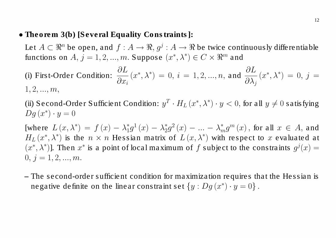
• Theorem 3(b) [Several Equality Constraints]:

Let A ⊂ <n be open, and f : A→ <, gj : A→ < be twice continuously differentiable

functions on A, j = 1, 2, ...,m. Suppose (x∗, λ∗) ∈ C ×<m and

(i) First-Order Condition:∂L

∂xi(x∗, λ∗) = 0, i = 1, 2, ..., n, and

∂L

∂λj(x∗, λ∗) = 0, j =

1, 2, ...,m,

(ii) Second-Order Sufficient Condition: yT ·HL (x∗, λ∗) · y < 0, for all y 6= 0 satisfying

Dg (x∗) · y = 0[where L (x, λ∗) = f (x) − λ∗1g

1 (x) − λ∗2g2 (x) − ... − λ∗mg

m (x) , for all x ∈ A, and

HL (x∗, λ∗) is the n × n Hessian matrix of L (x, λ∗) with respect to x evaluated at

(x∗, λ∗)]. Then x∗ is a point of local maximum of f subject to the constraints gj(x) =0, j = 1, 2, ...,m.

– The second-order sufficient condition for maximization requires that the Hessian is

negative definite on the linear constraint set {y : Dg (x∗) · y = 0} .

13

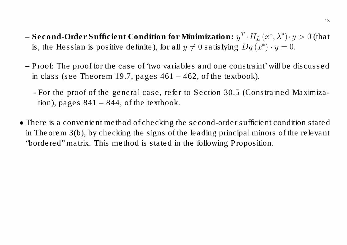
– Second-Order Sufficient Condition for Minimization: yT ·HL (x∗, λ∗) ·y > 0 (that

is, the Hessian is positive definite), for all y 6= 0 satisfying Dg (x∗) · y = 0.

– Proof: The proof for the case of ‘two variables and one constraint’ will be discussed

in class (see Theorem 19.7, pages 461 – 462, of the textbook).

- For the proof of the general case, refer to Section 30.5 (Constrained Maximiza-

tion), pages 841 – 844, of the textbook.

• There is a convenient method of checking the second-order sufficient condition stated

in Theorem 3(b), by checking the signs of the leading principal minors of the relevant

“bordered” matrix. This method is stated in the following Proposition.

14

• Proposition 1(b):

To determine the definiteness of a quadratic form of n variables, Q (x) = xTAx,when restricted to a constraint set given by m linear equations Bx = 0, construct the

(n +m) × (n +m) matrix S by bordering the matrix A above and to the left by the

coefficients B of the linear constraints:

S =

(0 BBT A

).

Check the signs of the last (n−m) leading principal minors of S, starting with the

determinant of S itself.

(a) If |S| has the same sign as (−1)n and if these last (n−m) leading principal minors

alternate in sign, then Q is negative definite on the constraint set Bx = 0.

(b) If |S| and these last (n−m) leading principal minors all have the same sign as

(−1)m, then Q is positive definite on the constraint set Bx = 0.

• For discussions on Propositions 1(a) and 1(b) refer to Section 16.3 (Linear Con-

straints and Bordered Matrices) (pages 386-393) of the textbook.

15

4. Sufficient Conditions for Constrained Global Maximumand Minimum

• Theorem 4:

Let A ⊂ <n be an open convex set, and f : A → <, gj : A → < be continuously

differentiable functions on A, j = 1, 2, ...,m. Suppose (x∗, λ∗) ∈ C×<m and Of (x∗) =λ∗1Og1(x∗) + λ∗2Og2(x∗) + ... + λ∗mOgm(x∗). If L (x, λ∗) = f (x)− λ∗1g1 (x)− λ∗2g2 (x)−... − λ∗mg

m (x) is concave (respectively, convex) in x on A, then x∗ is a point of

global maximum (respectively, minimum) of f subject to the constraints gj(x) = 0,j = 1, 2, ...,m.

– Proof: To be discussed in class.

16

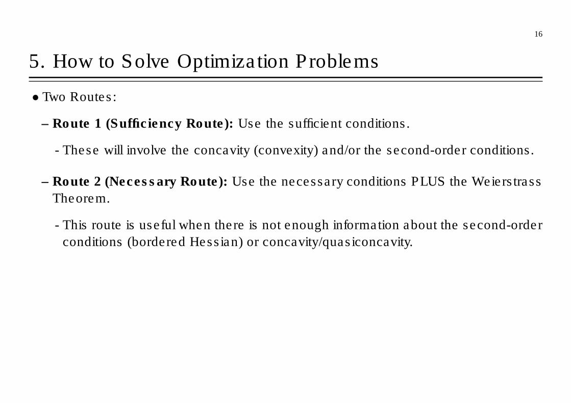
5. How to Solve Optimization Problems

• Two Routes:

– Route 1 (Sufficiency Route): Use the sufficient conditions.

- These will involve the concavity (convexity) and/or the second-order conditions.

– Route 2 (Necessary Route): Use the necessary conditions PLUS the Weierstrass

Theorem.

- This route is useful when there is not enough information about the second-order

conditions (bordered Hessian) or concavity/quasiconcavity.

17

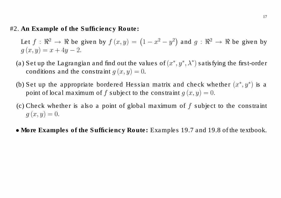
#2. An Example of the Sufficiency Route:

Let f : <2 → < be given by f (x, y) =(1− x2 − y2

)and g : <2 → < be given by

g (x, y) = x + 4y − 2.

(a) Set up the Lagrangian and find out the values of (x∗, y∗, λ∗) satisfying the first-order

conditions and the constraint g (x, y) = 0.

(b) Set up the appropriate bordered Hessian matrix and check whether (x∗, y∗) is a

point of local maximum of f subject to the constraint g (x, y) = 0.

(c) Check whether is also a point of global maximum of f subject to the constraint

g (x, y) = 0.

• More Examples of the Sufficiency Route: Examples 19.7 and 19.8 of the textbook.

18

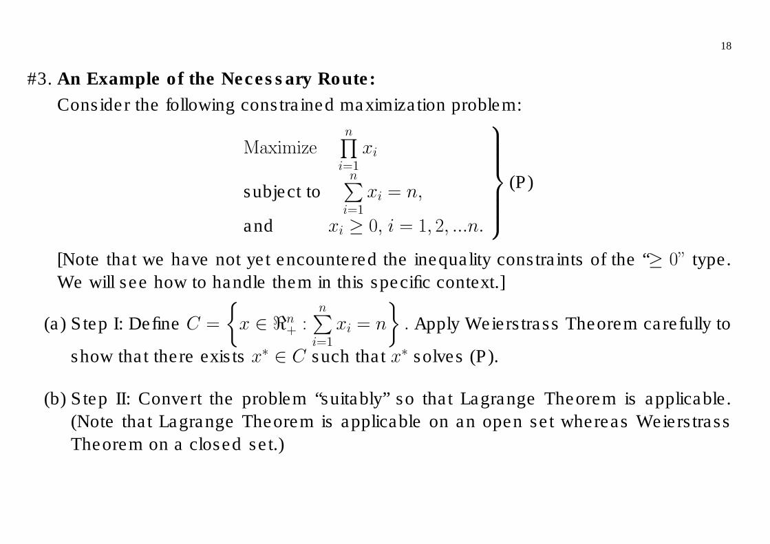
#3. An Example of the Necessary Route:

Consider the following constrained maximization problem:

Maximizen∏i=1

xi

subject ton∑i=1

xi = n,

and xi ≥ 0, i = 1, 2, ...n.

(P)

[Note that we have not yet encountered the inequality constraints of the “≥ 0” type.

We will see how to handle them in this specific context.]

(a) Step I: Define C =

{x ∈ <n+ :

n∑i=1

xi = n

}. Apply Weierstrass Theorem carefully to

show that there exists x∗ ∈ C such that x∗ solves (P).

(b) Step II: Convert the problem “suitably” so that Lagrange Theorem is applicable.

(Note that Lagrange Theorem is applicable on an open set whereas Weierstrass

Theorem on a closed set.)

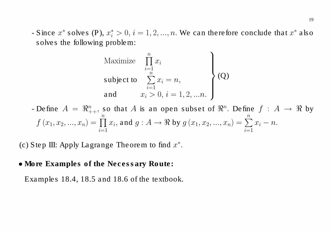
19

- Since x∗ solves (P), x∗i > 0, i = 1, 2, ..., n. We can therefore conclude that x∗ also

solves the following problem:

Maximizen∏i=1

xi

subject ton∑i=1

xi = n,

and xi > 0, i = 1, 2, ...n.

(Q)

- Define A = <n++, so that A is an open subset of <n. Define f : A → < by

f (x1, x2, ..., xn) =n∏i=1

xi, and g : A→ < by g (x1, x2, ..., xn) =n∑i=1

xi − n.

(c) Step III: Apply Lagrange Theorem to find x∗.

• More Examples of the Necessary Route:

Examples 18.4, 18.5 and 18.6 of the textbook.

20

References

• Must read the following sections from the textbook:

– Section 16.3 (pages 386 – 393): Linear Constraints and Bordered Matrices,

– Section 18.1 and 18.2 (pages 411 – 424): Equality Constraints,

– Section 19.3 (pages 457 – 469): Second-Order Conditions (skip the subsection on

Inequality Constraints for the time-being),

– Section 30.5 (pages 841 – 844): Constrained Maximization.

• This material is based on

1. Bartle, R., The Elements of Real Analysis, (chapter 7),

2. Apostol, T., Mathematical Analysis: A Modern Approach to Advanced Calculus,

(chapter 6).

3. Takayama, A., Mathematical Economics, (chapter 1).

21

• A proof of the important Proposition 1 can be found in

4. Mann, H.B., “Quadratic Forms with Linear Constraints”, American Mathematical

Monthly (1943), pages 430 – 433, and also in

5. Debreu, G., “Definite and Semidefinite Quadratic Forms”, Econometrica (1952),

pages 295 – 300.