classical mechanics - squarespace · pdf file1.1 kinematics and kinetics ... the law of action...
TRANSCRIPT
Classical Mechanics
Hyoungsoon Choi
Spring, 2014
Contents
1 Introduction 41.1 Kinematics and Kinetics . . . . . . . . . . . . . . . . . . . . . . . 51.2 Kinematics: Watching Wallace and Gromit . . . . . . . . . . . . 61.3 Inertia and Inertial Frame . . . . . . . . . . . . . . . . . . . . . . 8
2 Newton’s Laws of Motion 102.1 The First Law: The Law of Inertia . . . . . . . . . . . . . . . . . 102.2 The Second Law: The Equation of Motion . . . . . . . . . . . . . 112.3 The Third Law: The Law of Action and Reaction . . . . . . . . . 12
3 Laws of Conservation 143.1 Conservation of Momentum . . . . . . . . . . . . . . . . . . . . . 143.2 Conservation of Angular Momentum . . . . . . . . . . . . . . . . 153.3 Conservation of Energy . . . . . . . . . . . . . . . . . . . . . . . 17
3.3.1 Kinetic energy . . . . . . . . . . . . . . . . . . . . . . . . 173.3.2 Potential energy . . . . . . . . . . . . . . . . . . . . . . . 183.3.3 Mechanical energy conservation . . . . . . . . . . . . . . . 19
4 Solving Equation of Motions 204.1 Force-Free Motion . . . . . . . . . . . . . . . . . . . . . . . . . . 214.2 Constant Force Motion . . . . . . . . . . . . . . . . . . . . . . . . 22
4.2.1 Constant force motion in one dimension . . . . . . . . . . 224.2.2 Constant force motion in two dimensions . . . . . . . . . 23
4.3 Varying Force Motion . . . . . . . . . . . . . . . . . . . . . . . . 254.3.1 Drag force . . . . . . . . . . . . . . . . . . . . . . . . . . . 254.3.2 Harmonic oscillator . . . . . . . . . . . . . . . . . . . . . . 29
5 Lagrangian Mechanics 305.1 Configuration Space . . . . . . . . . . . . . . . . . . . . . . . . . 305.2 Lagrangian Equations of Motion . . . . . . . . . . . . . . . . . . 325.3 Generalized Coordinates . . . . . . . . . . . . . . . . . . . . . . . 345.4 Lagrangian Mechanics . . . . . . . . . . . . . . . . . . . . . . . . 365.5 D’Alembert’s Principle . . . . . . . . . . . . . . . . . . . . . . . . 375.6 Conjugate Variables . . . . . . . . . . . . . . . . . . . . . . . . . 39
1
CONTENTS 2
6 Hamiltonian Mechanics 406.1 Legendre Transformation: From Lagrangian to Hamiltonian . . . 406.2 Hamilton’s Equations . . . . . . . . . . . . . . . . . . . . . . . . 416.3 Configuration Space and Phase Space . . . . . . . . . . . . . . . 436.4 Hamiltonian and Energy . . . . . . . . . . . . . . . . . . . . . . . 45
7 Central Force Motion 477.1 Conservation Laws in Central Force Field . . . . . . . . . . . . . 477.2 The Path Equation . . . . . . . . . . . . . . . . . . . . . . . . . . 49
8 System of Multiparticles 518.1 Weighted Average . . . . . . . . . . . . . . . . . . . . . . . . . . 518.2 Center of Mass . . . . . . . . . . . . . . . . . . . . . . . . . . . . 528.3 Linear Momentum . . . . . . . . . . . . . . . . . . . . . . . . . . 538.4 Elastic Collisions of Two Particles . . . . . . . . . . . . . . . . . 548.5 Kinematics of Elastic Collisions . . . . . . . . . . . . . . . . . . . 568.6 Inelastic Collisions . . . . . . . . . . . . . . . . . . . . . . . . . . 578.7 Reduced Mass . . . . . . . . . . . . . . . . . . . . . . . . . . . . . 578.8 Scattering Cross Section . . . . . . . . . . . . . . . . . . . . . . . 598.9 Rutherford Scattering Formula . . . . . . . . . . . . . . . . . . . 638.10 Angular Momentum . . . . . . . . . . . . . . . . . . . . . . . . . 638.11 Energy of the System . . . . . . . . . . . . . . . . . . . . . . . . 64
9 Rigid Body Kinematics 679.1 Rotation and Linear Velocity . . . . . . . . . . . . . . . . . . . . 679.2 Moment of Inertia Tensor . . . . . . . . . . . . . . . . . . . . . . 689.3 Kinetic Energy . . . . . . . . . . . . . . . . . . . . . . . . . . . . 709.4 Rigid Body Kinematics . . . . . . . . . . . . . . . . . . . . . . . 709.5 Principal Axes of Inertia . . . . . . . . . . . . . . . . . . . . . . . 719.6 Moments of Inertia for Different Body Coordinate Systems . . . 739.7 Euler’s Equations . . . . . . . . . . . . . . . . . . . . . . . . . . . 749.8 Free Body Rotation of a Rigid Body with Axial Symmetry . . . 759.9 Precession of a Symmetric Top due to a Weak Torque . . . . . . 769.10 Steady Precession of a Symmetric Top under a Uniform Torque . 779.11 Eulerian Angles . . . . . . . . . . . . . . . . . . . . . . . . . . . . 789.12 Motion of a Symmetric Top with One Point Fixed . . . . . . . . 80
CONTENTS 3
Disclaimer: The world view represented in this section only holdsfor Newtonian physics and Galileian relativity. However, it is stillvery useful in developing physical intuitions relevant to classical me-chanics. Basically, I will be treating you like a person born pre 1900,before quantum mechanics and special relativity.

Chapter 1
Introduction
Unlike quantum mechanics, in which our intuitive world view breaks down com-pletely from the get go, there is no big secret in classical mechanics. The objectsyou are interested in are mostly visible and they respond to a push or pull, tech-nically known as the force. The question here is ”how do the objects moveunder given set of forces?” At the end of the day, your answer will be given asthe position of an object as a function of time.
To achieve this goal, everything you learn in classical mechanics boils downto understanding the consequences of a single equation, F = ma. We will notpretend that this is a completely new concept you are yet to learn. Instead,we will deal with it exactly as what it is, something you have learned already,of which you do not understand the full consequences yet. In other words,throughout this course, we will learn how to interpret the equation and itsconsequences more carefully through various examples.
But before we seriously delve into mechanics, let’s take a brief trip to France.In Sevres, France, there is an underground vault that holds big chunks of metalthat are made out of 90% platinum and10% iridium. There are three keys tothis vault and you need all three to get in. Each year three people holdingthe keys to this vault gather together, go down to the vault open it up andmake sure these metal chunks are still there unaltered. This seemingly bizarrebehavior that can be mistaken as a ritual by platinum-iridium worshipping cultis actually of utmost importance to us that study science, especially physics.
The vault actually belongs to the International Bureau for Weights andMeasures (Bureau International des Poids et Mesures, BIPM), and those metalpieces are the international prototype kilogram (IPK) and the internationalprototype meter (IPM). The sole purpose of BIPM’s existence is to define akilometer, a meter (and a second) and IPK and IPM are exactly that. Thereisn’t any international prototype second (IPS) in that vault only because thereis simply no physical object that can represent time. Now, what does this haveanything to do with what we are about to study? As we will soon see, morethan what you can imagine.
4
CHAPTER 1. INTRODUCTION 5
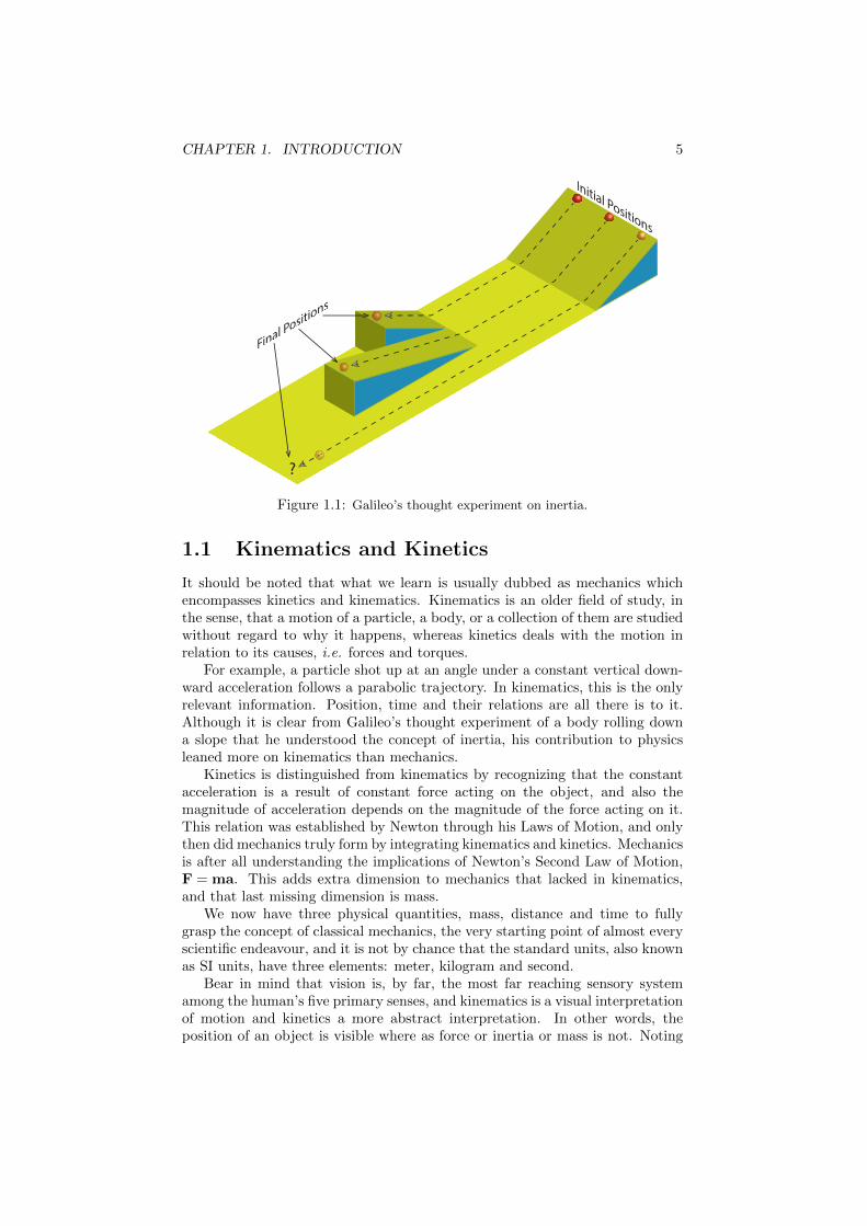
?
Figure 1.1: Galileo’s thought experiment on inertia.
1.1 Kinematics and Kinetics
It should be noted that what we learn is usually dubbed as mechanics whichencompasses kinetics and kinematics. Kinematics is an older field of study, inthe sense, that a motion of a particle, a body, or a collection of them are studiedwithout regard to why it happens, whereas kinetics deals with the motion inrelation to its causes, i.e. forces and torques.
For example, a particle shot up at an angle under a constant vertical down-ward acceleration follows a parabolic trajectory. In kinematics, this is the onlyrelevant information. Position, time and their relations are all there is to it.Although it is clear from Galileo’s thought experiment of a body rolling downa slope that he understood the concept of inertia, his contribution to physicsleaned more on kinematics than mechanics.
Kinetics is distinguished from kinematics by recognizing that the constantacceleration is a result of constant force acting on the object, and also themagnitude of acceleration depends on the magnitude of the force acting on it.This relation was established by Newton through his Laws of Motion, and onlythen did mechanics truly form by integrating kinematics and kinetics. Mechanicsis after all understanding the implications of Newton’s Second Law of Motion,F = ma. This adds extra dimension to mechanics that lacked in kinematics,and that last missing dimension is mass.
We now have three physical quantities, mass, distance and time to fullygrasp the concept of classical mechanics, the very starting point of almost everyscientific endeavour, and it is not by chance that the standard units, also knownas SI units, have three elements: meter, kilogram and second.
Bear in mind that vision is, by far, the most far reaching sensory systemamong the human’s five primary senses, and kinematics is a visual interpretationof motion and kinetics a more abstract interpretation. In other words, theposition of an object is visible where as force or inertia or mass is not. Noting
CHAPTER 1. INTRODUCTION 6
where the Sun, the Moon and stars each day was a relatively simple task. Sincetime is, as we shall soon see, a measure of change, any change in position thatwe observe already includes the notion of time. In other words, observation ofpositional change is the kinematics itself. When we are observing objects, saystars in the sky, move, we are probing into its kinematics already. Why theywere there when they were there was a lot more tricky business. And exactlyfor this reason, we start with kinematics.
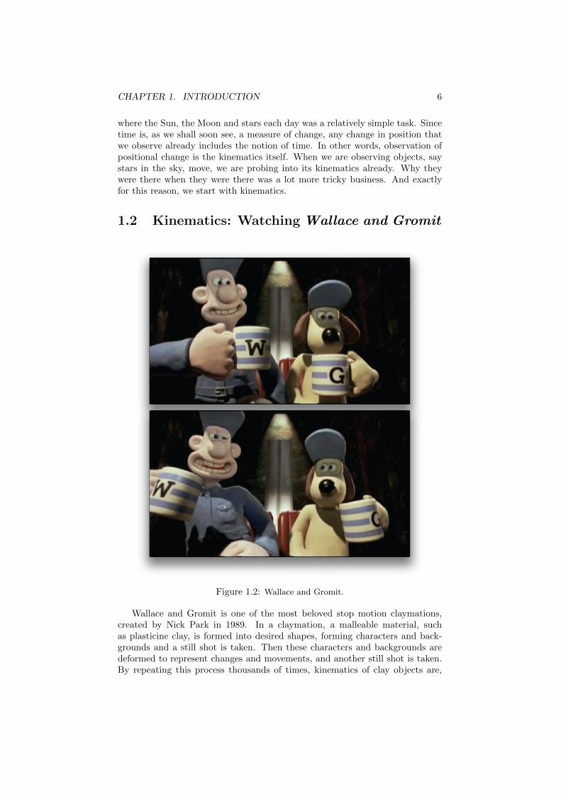
1.2 Kinematics: Watching Wallace and Gromit
Figure 1.2: Wallace and Gromit.
Wallace and Gromit is one of the most beloved stop motion claymations,created by Nick Park in 1989. In a claymation, a malleable material, suchas plasticine clay, is formed into desired shapes, forming characters and back-grounds and a still shot is taken. Then these characters and backgrounds aredeformed to represent changes and movements, and another still shot is taken.By repeating this process thousands of times, kinematics of clay objects are,

CHAPTER 1. INTRODUCTION 7
well, fabricated. Nonetheless, it does allow us to peek into the key concepts inkinematics.
Suppose, the plasticine clay is formed into shapes and you take a still shot.After a few hours, you take another still shot, another after a few hours, andanother and another and so on. The clay won’t move itself and when you playa movie out of these still shots, you will end up with a very boring movie. Noone would notice, if you pause the video during the showing of that movie, thatis of course, if there is anyone coming to see this. Just by staring at this, noone would be able to tell what happens before what. In that little claymationuniverse, the time doesn’t exist.
Time takes any meaning only if there are changes; something has to move.Let’s take a look at two images in Fig. 1.2. We can tell by looking at them thatthey are not the same. Then how far did Wallace’s cup move? By about thewidth of the cup. But how far is it? Is it big or small? If you try to answer thisquestion, what you learn is that there is no absolute scale of length in physics.When you say the cup moved by the width of the cup, you are setting the sizeof the cup as the reference scale. Once you decide to use the size of the cup asyour unit of length measurements, you can now say something has moved bythree cups or eleven cups, etc.
However, spatial change alone is not sufficient to describe motion. The factthat the position of some objects changed self-creates this other dimension,time. Unless you are willing to accept the notion that an object can be attwo different places at the same time, which you can’t in classical physics, thefact that there is a change in position allows you to conclude only that thesetwo images represent two different points in time. But, because you can neverfigure out how far apart in time these images are by simply looking at them,the concept of time exists, but not in truly meaningful way. Just like length,there is no absolute measure of time. To quantify, how much time has elapsed,you need to be able to compare changes.
Imagine an independently moving object, say a red ball moving from pointA to point B. Even if we cannot tell in any absolute sense how long it took forthe cup to move, we can say whether it took longer than the red ball to movefrom point A to point B. However, the point of reference vanishes as soon as thered ball stops moving. For this reason, it is better to pick a repetitive motionas a reference of time, such as the Earth’s rotation or orbital motion around theSun. We can then use one cycle of this motion as a unit of time and describeother objects’ motion based on it. For example, we can say that Wallace’s cuphas moved by one and a half cup in 1/864000 of the Earth’s rotation whereasGromit’s cup has moved by 0.8 cup in the same period of time, thereby Wallace’scup moved at a higher velocity.
This is precisely why we need IPK and IPS. Only after having a referencepoint for distance and time, such as the width of the cup and the duration ofthe Earth’s one full rotation, can we define what motions are quantitativelyand kinematics starts to make sense. IPM and IPS (if there was one) arethe internationally agreed upon basis for this relativeness, and that is why itis so important to have a precise, easily reproducible definition of them andkeep them unaltered. Currently, one meter is defined as the length of the pathtravelled by light in vacuum during a time interval of 1/299,792,458 of a second.One second is defined as the duration of 9,192,631,770 periods of the radiationcorresponding to the transition between the two hyperfine levels of the ground

CHAPTER 1. INTRODUCTION 8
state of the caesium 133 atom. We will learn how IPK is related to mechanics,shortly, but at this point, it is not too big a stretch to say that our understandingof mechanics is kept in that vault in France.
Now that we have established the concept of time and space, motion hasa meaning. We can define velocity and acceleration, as the amount change inposition in a given time and the amount of change of that change in a given time.The agreement on that time frame is what allows you to create claymations.In real life, it can take a really long time to create two successive shots. Butbecause you set the time difference between any two successive shots equal whenyou are playing it in video, you can create a controlled motion, and suddenlythe movie gets a life and becomes a form of entertainment, and also a subjectof kinematics.
1.3 Inertia and Inertial Frame
Unlike length and time, mass is not a visually identifiable quantity. So thequestion follows: how do we identify mass? But this question is in fact, missinga more important point entirely: why do we even care about mass? Kinemat-ics, such as the famous Kepler’s Laws of planetary motion, can be sufficientlydescribed by space and time. Mass and motion at first glance are unrelated.However, if we want to describe the origin or root cause of such a motion, thatis when we get into trouble. To answer this question adequately, we have tofirst understand what inertia is.
The concept of force goes back to ancient Greece, when Archemedes al-ready seemed to grasp the vector nature of force with Eucledian geometry andtrigonometry. Such methods were very effective at describing statics. The prob-lem was that their understanding of kinetics was deeply flawed. Aristotle arguedthat for something to move, force has to be applied and the speed of an object’smotion is proportional to the applied force and inversely proportional to theviscosity of the surrounding medium. It is obvious that they knew motion andforce were related, but they simply had no clue what that somehow was.
The problem with this reasoning is that, well there are just so many thatI don’t even know where to start. It is Galileo’s brilliant insight on inertia(Fig. 1.1) that allowed us to view the relationship between motion and force ona completely different light. He argued that every object has a natural tendencyto maintain its motion, and a motion of the object will be unaltered unless thereis net force acting on it. This tendency to maintain its motion is called inertia,and this is why we care about mass. But we will get to this point in the nextchapter.
Another important contribution of Galileo is that he singled out constantvelocity motion from all other motions, yet recognized that all constant velocitymotion can be grouped as one indistinguishable set regardless of what thatvelocity is. From this, the concept of inertial frame was born.
Imagine a reference frame S that we can declare as absolutely not moving.Within this frame, an object, say a hockey puck, is moving at a constant velocityvp. An observer within the reference frame would see the motion of the hockeypuck as free of any outside influence. Now imagine a moving frame S′ at avelocity vS′ relative to the fixed frame S. Then to an observer within the S′
frame, the hockey puck slides at a velocity vp − vS′ , which is also a constant
CHAPTER 1. INTRODUCTION 9
velocity. Thus the observer in the S′ frame would see the motion of the puckalso free of outside influence. Despite the difference in velocity, both observerswould see the effect of inertia, that is the hockey puck continues its originalmotion. For this reason, frames moving with a constant velocity is referred toas inertial frame. We will discuss the importance of this in more detail in thenext chapter.
Chapter 2
Newton’s Laws of Motion
With his concept of inertia, Galileo emphasized the importance of constant ve-locity motion. What Newton, in turn, did was to build upon that and emphasizethe role of force, the physical quantity that is required to resist inertia. He thencame up with three Laws of Motion. In its original form, they read:
Lex I: Corpus omne perseverare in statu suo quiescendi vel movendi unifor-miter in directum, nisi quatenus a viribus impressis cogitur statum illummutare.
Lex II: Mutationem motus proportionalem esse vi motrici impressae, et fierisecundum lineam rectam qua vis illa imprimitur.
Lex III: Actioni contrariam semper et qualem esse reactionem: sive corporumduorum actiones in se mutuo semper esse quales et in partes contrariasdirigi.
Now, in a language that we can understand, what they are saying are these:
Law I: Every body persists in its state of being at rest or of moving uniformlystraight forward, except insofar as it is compelled to change its state byforce impressed.
Law II: The change of momentum of a body is proportional to the impulseimpressed on the body, and happens along the straight line on which thatimpulse is impressed.
Law III: To every action there is always an equal and opposite reaction: orthe forces of two bodies on each other are always equal and are directed inopposite directions.
OK, this may not be so understandable either. So, we will delve into them oneby one more carefully.
2.1 The First Law: The Law of Inertia
Law I: Every body persists in its state of being at rest or of moving uniformlystraight forward, except insofar as it is compelled to change its state byforce impressed.
10

CHAPTER 2. NEWTON’S LAWS OF MOTION 11
All three laws that are seemingly stating different facts can be compressedinto a single equation:
F =dp
dt= ma (2.1)
This equation is called the equation of motion and it is, without a doubt, thesingle most important equation in classical mechanics. In fact, it can be saidthat this equation alone is all of classical mechanics. Throughout the year, wewill learn a number of different applications of this single equation.
Then the question arises: why did of all the people, Newton, who probablyknew better than anyone else that the laws can be compressed as a single equa-tion, bothered to elaborate in such detail? For example, the first law seems tobe, at first glance, a reiteration of the second law: from F = ma, it is quiteobvious that when no force is applied (F = 0), the object cannot accelerate nordecelerate.
However, it deserves to stand on its own for one very important reason wehave already discussed in Chapter 1. It allows us to identify inertia and, equallyimportantly, set up a useful reference frame, the inertial frame. We can defineinertial frame as
Definition: Inertial Frame is a reference frame in which the First Law holds.
As we shall soon see, only within the inertial frame, is the equation of motionmeaningful.
Also, even though the first law seems to be a subset of more general secondlaw, it is a very distinct subset in the sense that at zero acceleration, the conceptof mass is completely meaningless. Because force-free motion is by definition,well, force-free, the object has no net-interaction with anything. Because theobject is interactionless, you cannot distinguish a more massive object from aless massive object in this force free environment.
When you are staring at two different objects moving at two different veloc-ities, it maybe tempting to conclude that one is lighter than the other becausethis is moving slower than that. However tempting it may be, you simply can-not.
Imagine you, your friend and two balls constitute the entire universe. Youare sitting still (or so you think) and your friend is moving at a velocity of 5m/s away from you to your right. Two balls are moving in opposite directions,a red one to your left at 1 m/s, a blue one to your right at 4 m/s. To you, ablue ball moves faster than the red. But for your friend, the red ball moves at 6m/s and the blue one at 1 m/s, both to his left. For him, the red ball is movingfaster.
Unless you are willing to accept the notion that two balls can have differentmass for two different people, we now have a problem when you try to interpretphysical world based on velocity. Velocity just allows you to establish relativereference frame against one another but the role of velocity stops right there(until you learn Einstein’s relativity, but that is a whole new story).
2.2 The Second Law: The Equation of Motion
Law II: The change of momentum of a body is proportional to the impulseimpressed on the body, and happens along the straight line on which that

CHAPTER 2. NEWTON’S LAWS OF MOTION 12
impulse is impressed.
The first law hints at the concept of force, but the second law is the onethat explicitly defines force. Mathematically expressing the original statementof the above Law II, we get
P = ∆p (2.2)
Newton appropriately defined momentum p of an object to be a quantity pro-portional to its velocity, i.e. p = mv and an impulse P occurs when a force Facts over an interval of time ∆t, i.e. P =
∫∆t
Fdt. Then the Eq. (2.2) can berewritten as ∫
∆t
Fdt = ∆(mv)
F =d(mv)
dt= m
dv
dt= ma (2.3)
Eq. (3.12) is where the equation of motion, Eq. (2.1) directly comes out of,and we can see that the net force applied to a body produces a proportionalacceleration.
Also, the proportionality constant, m, between the velocity and momentumis of great significance here. From Eq. (2.1), we can see that for a given amountof force, acceleration is inversely proportional to m. In other words, the largerm is, the greater the tendency to stay its course of motion. To put it anotherway, m is the physical quantity that represents inertia i.e. mass.
From this definition of mass, we can see that measurement of force can beused to measure mass. A balance is an excellent example. Any balance usesbalancing between the known amount of force and a force acting on an objectof unknown mass, . e.g. gravitational force.
For what we will learn throughout this course, however, there is a morecomplicated use for the Newton’s Second Law. If we assume that the mass mdoes not vary with time, Newton’s equation of motion, F = ma = mr, is simplya second-order differential equation that may be integrated to find r = r(t) ifthe function F is known. Specifying the initial values of r and r = v then allowsus to evaluate the two arbitrary constants of integration. We then determinethe motion of a particle by the force function F and the initial values of positionr and velocity v.
2.3 The Third Law: The Law of Action and Re-action
Law III: To every action there is always an equal and opposite reaction: orthe forces of two bodies on each other are always equal and are directed inopposite directions.
The third and final of Newton’s laws is also known as the action-reactionlaw. In some sense, the first two laws were discovered already by Galileo andin fact none other than Newton himself gave credit to Galileo for the first law.However, the third law is the product of Newton’s great insight that all forcesare interactions between different bodies, and thus that there is no such thing

CHAPTER 2. NEWTON’S LAWS OF MOTION 13
F1
F2
F1
F2
(a) (b)
Figure 2.1: The Third Law of Motion in its (a) weak form and (b) strongform. In (a), there is no net force, but net torque is present.
as a unidirectional force or a force that acts on only one body. Whenever afirst body exerts a force F1 on a second body, the second body exerts a forceF2 = −F1 on the first body.
We can categorize the third law into two, a weak law of action-reaction anda strong law. In a weak form of the law, the action and reaction forces onlyhas to be equal in magnitude and opposite in direction. They need not lie on astraight line connecting the two particles or objects. As a result, there could bea net torque acting on the system. On the other hand, the strong form of thelaw states that the forces have to be lined up. This distinction may be trivial,but it will become important in the next chapter.
For the time being, we will rewrite the third law, using the definition of forcegiven by the second law,
dp1
dt= −dp2
dtm1a1 = −m2a2m2
m1= −a1
a2(2.4)
and from this we can give a practical definition of mass. If we set m1 as theunit mass, then, by comparing the ratio of accelerations when m1 is allowed tointeract with any other body, we can determine the mass of the other body. Soit is the Newton’s Laws that allows us to define relative mass to our selectionof unit mass m1.
Of course, to measure the accelerations, we must have appropriate clocks andmeasuring rods. Let’s now go back to IPK, IPM and IPS, these are basically theunit mass, a measuring rod and an appropriate clock required. From this, wecan see that the job of BIPM and classical mechanics are not separable. HavingIPM and IPS is what lets us to describe motion in a quantitative manner, andthat in turn, according to the Newton’s Laws, gives us the definition of mass.
Chapter 3
Laws of Conservation
In physics, there are a number of conservation laws, laws that state certainproperties of a system does not change in time. Laws of conservation is relatedto differentiable symmetries of physical systems, as Emmy Noether pointed out,and can be a subject of intense study. However, we will not delve into thispoint too deeply, at least not yet, and will cover three widely used conservationlaws that are direct consequences of Newton’s Laws of Motion. These three areconservation of momentum, angular momentum and energy. We will look intothese one by one.
3.1 Conservation of Momentum
Since the momentum is defined as the product of mass and velocity, for a systemthat conserves its mass, constant velocity is equivalent to constant momentum.Therefore, the concept of inertia stated in the First Law of Motion, in andof itself, is declaration of momentum conservation. Momentum conservation,however, extends beyond the force-free motion.
Imagine a particle that is accelerating. For this particle to accelerate, forcehas to be exerted. From the third law, when a force is acting on an object, therehas to be an entity that is exerting the force, and the first object in questionhas to apply the same amount of force in opposite direction on to that entity.In a mathematical form: F2 = −F1.
The equation can be rewritten as follows:
F1 + F2 = 0dp1
dt + dp2
dt = ddt (p1 + p2) = 0
∴ p1 + p2 = constant (3.1)
In other words, in the absence of external force, the total momentum of the twoobjects that are exchanging force is constant. The same logic can be appliedto a multi-object system beyond two objects. It follows that, at least classicalmechanically, total momentum of the universe is conserved. However, this is nota practically useful statement. What this implies is that an external force ona system is always an internal force of a larger system, and in reality, studyingmechanics comes down to isolating an observable systems appropriately.
14
CHAPTER 3. LAWS OF CONSERVATION 15
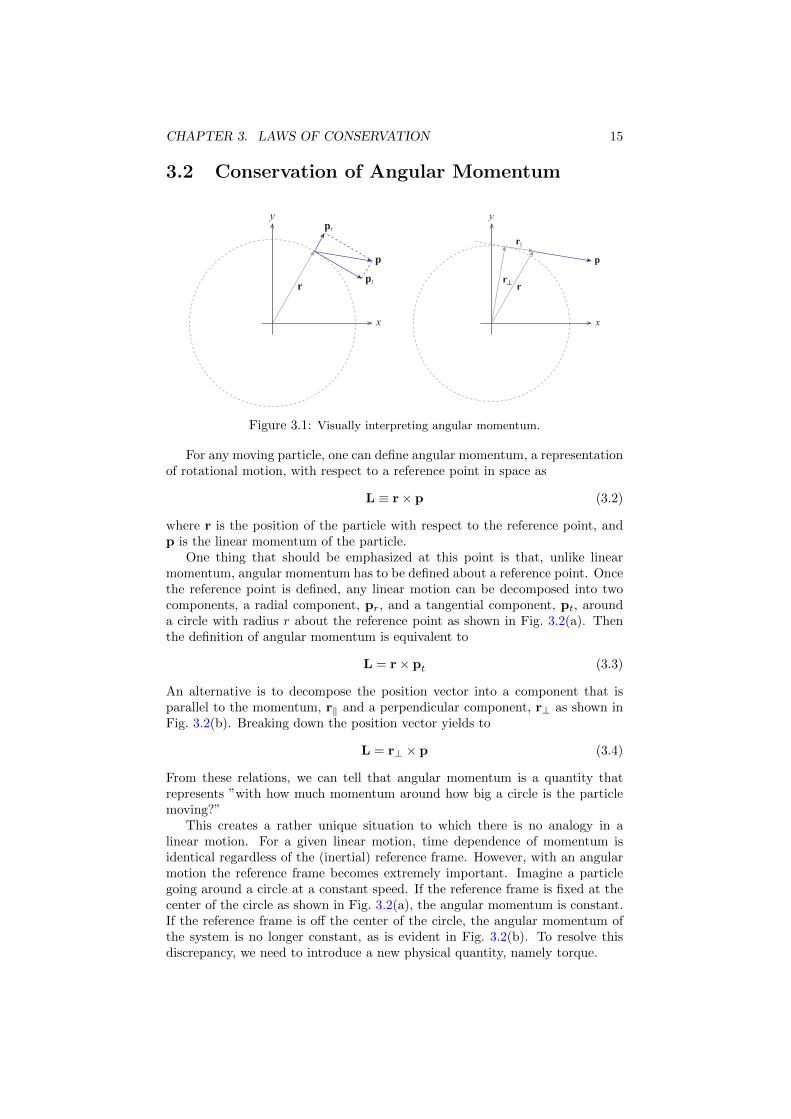
3.2 Conservation of Angular Momentum
p
pr
ptr
x
y
p
r
x
y
r||
r
Figure 3.1: Visually interpreting angular momentum.
For any moving particle, one can define angular momentum, a representationof rotational motion, with respect to a reference point in space as
L ≡ r× p (3.2)
where r is the position of the particle with respect to the reference point, andp is the linear momentum of the particle.
One thing that should be emphasized at this point is that, unlike linearmomentum, angular momentum has to be defined about a reference point. Oncethe reference point is defined, any linear motion can be decomposed into twocomponents, a radial component, pr, and a tangential component, pt, arounda circle with radius r about the reference point as shown in Fig. 3.2(a). Thenthe definition of angular momentum is equivalent to
L = r× pt (3.3)
An alternative is to decompose the position vector into a component that isparallel to the momentum, r‖ and a perpendicular component, r⊥ as shown inFig. 3.2(b). Breaking down the position vector yields to
L = r⊥ × p (3.4)
From these relations, we can tell that angular momentum is a quantity thatrepresents ”with how much momentum around how big a circle is the particlemoving?”
This creates a rather unique situation to which there is no analogy in alinear motion. For a given linear motion, time dependence of momentum isidentical regardless of the (inertial) reference frame. However, with an angularmotion the reference frame becomes extremely important. Imagine a particlegoing around a circle at a constant speed. If the reference frame is fixed at thecenter of the circle as shown in Fig. 3.2(a), the angular momentum is constant.If the reference frame is off the center of the circle, the angular momentum ofthe system is no longer constant, as is evident in Fig. 3.2(b). To resolve thisdiscrepancy, we need to introduce a new physical quantity, namely torque.
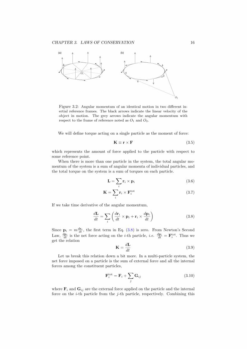
CHAPTER 3. LAWS OF CONSERVATION 16
(a) (b)
O1
O2
Figure 3.2: Angular momentum of an identical motion in two different in-ertial reference frames. The black arrows indicate the linear velocity of theobject in motion. The grey arrows indicate the angular momentum withrespect to the frame of reference noted as O1 and O2.
We will define torque acting on a single particle as the moment of force:
K ≡ r× F (3.5)
which represents the amount of force applied to the particle with respect tosome reference point.
When there is more than one particle in the system, the total angular mo-mentum of the system is a sum of angular momenta of individual particles, andthe total torque on the system is a sum of torques on each particle.
L =∑i
ri × pi (3.6)
K =∑i
ri × Ftoti (3.7)
If we take time derivative of the angular momentum,
dL
dt=∑i
(dridt× pi + ri ×
dpidt
)(3.8)
Since pi = mdridt , the first term in Eq. (3.8) is zero. From Newton’s Second
Law, dpidt is the net force acting on the i-th particle, i.e. dpi
dt = Ftoti . Thus we
get the relation
K =dL
dt(3.9)
Let us break this relation down a bit more. In a multi-particle system, thenet force imposed on a particle is the sum of external force and all the internalforces among the constituent particles,
Ftoti = Fi +
∑j
Gij (3.10)
where Fi and Gij are the external force applied on the particle and the internalforce on the i-th particle from the j-th particle, respectively. Combining this
CHAPTER 3. LAWS OF CONSERVATION 17
result with the Newton’s Third Law, i.e. Gij = −Gji, Eq. (3.8) can be rewrittenas
dL
dt=
∑i
ri × Fi +∑i,j
ri ×Gij
=∑i
ri × Fi +∑i<j
(ri ×Gij + rj ×Gji)
=∑i
ri × Fi +∑i<j
(ri − rj)×Gij
=∑i
Ki +∑i<j
(ri − rj)×Gij (3.11)
The second term in the Eq. (3.11) is an internal torque. What is interestinghere is that the internal torque vanishes only if either there are no internalforces Gij = 0 or ri − rj is in the same direction as Gij , that is the internalforces are along the lines connecting the two particles. In other words, if theinternal forces are present, the internal torque vanishes only if the strong formof Newton’s Third Law holds. For almost all the problems that we will dealwith throughout this course, the strong form actually holds, so you need not toworry about this subtle distinction.
In such cases, the total angular momentum of a particle system does notchange with time in the absence of an external torque. In other words, theangular momentum is conserved.
3.3 Conservation of Energy
Conservation energy is one of the fundamental conservation laws of nature. Itshould be a concept you must have learned since middle school and be familiarwith by now. However, the fact that energy, unlike momentum or angularmomentum, takes many forms makes the law of conservation of energy not astrivial as one might think at first. In light of these facts, it should come as nosurprise that Newton never mentioned energy in his work.
Nonetheless, one cannot simply look over the importance of the energy con-servation. Within the framework of classical mechanics, conservation of energyrefers to lossless transfer of energy between two very specific forms of energy:kinetic energy and potential energy. So the first step here would be to definethese two types of energy.
3.3.1 Kinetic energy
Let us start from the Second Law of Motion:
F = mdv
dt(3.12)
We need not define or restrict the type of force F, and it can be considered simplyas the net force acting on the particle of interest. Take the scalar product ofEq. (3.12) with v, and we get
F · v = mdv
dt· v =
d
dt
(1
2mv · v
)(3.13)
CHAPTER 3. LAWS OF CONSERVATION 18
By defining T = 12mv
2, we can rewrite the above equation as
T2 − T1 =
∫ t2
t1
F · vdt (3.14)
When F is a force field F(r), that is the amount of force F acting on the particleis given for each position r, the right hand side of the Eq. (3.14) becomes∫ t2
t1
F · vdt =
∫ t2
t1
F(r) · drdtdt =
∫C
F(r) · dr = W12 (3.15)
which is the work done by moving the particle across the fixed path C from pointr1 to r2 during the time between t2 and t1. (See Fig. 3.3.1.) Since the righthand side of the Eq. (3.14) represents work done on a particle, the left handside must represent a change in energy in the form of T = 1
2mv2. Because this
energy T represents the energy stored in a particle’s motion, that is T dependson m and v, we define T as the kinetic energy, the energy of motion.
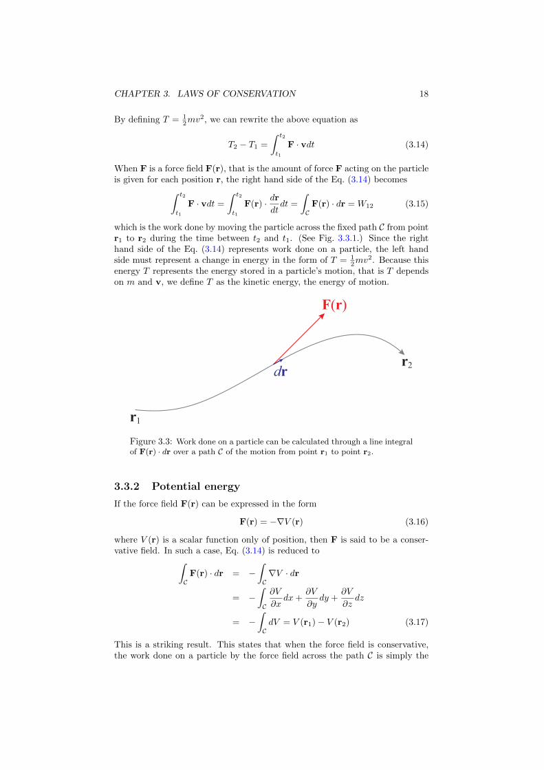
F(r)
dr
r1
r2
Figure 3.3: Work done on a particle can be calculated through a line integralof F(r) · dr over a path C of the motion from point r1 to point r2.
3.3.2 Potential energy
If the force field F(r) can be expressed in the form
F(r) = −∇V (r) (3.16)
where V (r) is a scalar function only of position, then F is said to be a conser-vative field. In such a case, Eq. (3.14) is reduced to∫
CF(r) · dr = −
∫C∇V · dr
= −∫C
∂V
∂xdx+
∂V
∂ydy +
∂V
∂zdz
= −∫CdV = V (r1)− V (r2) (3.17)
This is a striking result. This states that when the force field is conservative,the work done on a particle by the force field across the path C is simply the

CHAPTER 3. LAWS OF CONSERVATION 19
difference between a scalar field V (r) at the initial and final points of the pathC. The function V (r) is a form of energy that is stored in its position, and isusually referred to as the potential energy.
3.3.3 Mechanical energy conservation
From the relation between the kinetic energy and work, and the potential energyand work, we can find the following relationship for a particle under the influenceof a conservative force:
W12 = T2 − T1 = V1 − V2 (3.18)
and rewriting this equation, we get
T1 + V1 = T2 + V2 (3.19)
Because the choice of initial and final time and position, t1, t2, r1 and r2 isarbitrary, the above equation is equivalent to saying that the mechanical energy,i.e. the sum of kinetic and potential energy, is constant in time:
T + V = E = constant (3.20)
Simply put, the mechanical energy is conserved for a particle moving in a con-servative force field.
An important and very useful property of this energy conservation is thatbecause the potential energy is a function only of the position of the particle,the path it follows becomes irrelevant. Put in another way, even if the particleis under a geometrical constraint, e.g. a pendulum attached to a string or amarble rolling down a guide rail, if the constraint forces on the particle do nowork on the particle, the mechanical energy is still conserved.
Chapter 4
Solving Equation ofMotions
The starting point of classical mechanics is the equation of motion given by
F = ma (4.1)
Since, at the end of the day, what we want to find out in classical mechanics istime evolution of position of a physical object, r(t), the above equation turnsout to be a differential equation of the form
md2r
dt2− F(r, t) = 0 (4.2)
In some rare occasions, the force F(r, t) may contain higher order derivatives ofr with respect to t. But, as I said, this is very rare, especially in undergraduatephysics level, and for the most part, the equation of motion is a second orderdifferential equation.
If F(r, t) takes the form
F(r, t) = f2(t)d2r
dt2+ f1(t)
dr
dt+ f0(t)r + f(t) (4.3)
we can rewrite Eq. (4.2) as
a2(t)d2r
dt2+ a1(t)
dr
dt+ a0(t)r = f(t) (4.4)
where a2(t) = m − f2(t), a1(t) = −f1(t) and a0(t) = −f0(t). Aside from thefact that it is a vector equation, Eq. (4.4) has the same form as a linear n-thorder differential equation
an(x)dny
dxn+ an−1(x)
dn−1y
dxn−1+ · · ·+ a1(x)
dy
dx+ a0(x)y = f(x) (4.5)
where ai(x)’s and f(x) depend only on x.
20

CHAPTER 4. SOLVING EQUATION OF MOTIONS 21
4.1 Force-Free Motion
Let us first consider a one dimensional force-free motion with F (x, t) = 0. FromEq. (4.2), we get the equation of motion
md2x
dt2= 0 (4.6)
By defining v ≡ dx/dt, the equation reduces to a first order differential equation
dv
dt= 0 (4.7)
A fairly straightforward integration yields the following result
v =
∫ (dv
dt
)dt =
∫dv = v0 (4.8)
Since v = dx/dt, we can rewrite the above equation as
dx
dt= v0 (4.9)
Following the same procedure as Eq. (4.8), we get
x =
∫ (dx
dt
)dt =
∫v0dt = v0t+ x0 (4.10)
Here, x0 and v0 are unspecified constants. The position changes with time alonga straight line as shown in Fig. 4.1.
Time
Position
Figure 4.1: One dimensional force-free motion.
In this case, its starting point (y-intercept on the graph) and velocity (slope)are unknown, however, if the initial conditions x0 and v0 are specified, we canuniquely pick out a single line among infinitely many possibilities.

CHAPTER 4. SOLVING EQUATION OF MOTIONS 22
This method can be generalized to higher dimensional space, and one willget a solution of the form
r = v0t+ r0 (4.11)
In this case, although unfortunate choice of coordinate system might force youto have to solve a set of three identical differential equations for this problem, infact, an appropriate choice of coordinate system can always reduce the problemto a one dimensional problem.
4.2 Constant Force Motion
We now turn on a constant external force, F(r, t) = F0 on to this particle. But,we will once again start with one dimensional motion.
4.2.1 Constant force motion in one dimension
One dimensional constant force motion can be expressed by the equation ofmotion:
d2x
dt2=F0
m= a0 (4.12)
Same method used in the previous section can be utilized to find the solutionto this equation, and one can easily find that the solution is
x =1
2a0t
2 + v0t+ x0 (4.13)
Time
Position
Figure 4.2: A general solution to one dimensional constant force motion.
The solution has an additional term 12a0t
2, which is the effect of accelerationdue to the force. The solution is no longer a straight line. Instead, we get a
CHAPTER 4. SOLVING EQUATION OF MOTIONS 23
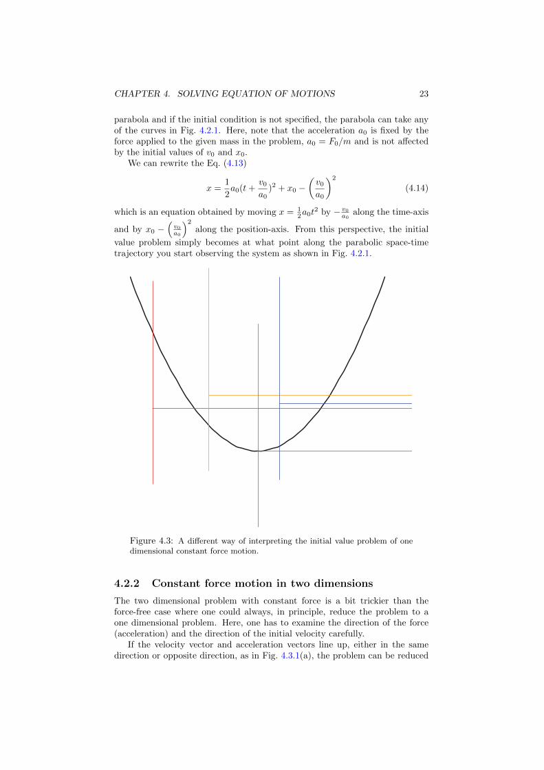
parabola and if the initial condition is not specified, the parabola can take anyof the curves in Fig. 4.2.1. Here, note that the acceleration a0 is fixed by theforce applied to the given mass in the problem, a0 = F0/m and is not affectedby the initial values of v0 and x0.
We can rewrite the Eq. (4.13)
x =1
2a0(t+
v0
a0)2 + x0 −
(v0
a0
)2
(4.14)
which is an equation obtained by moving x = 12a0t
2 by − v0a0
along the time-axis
and by x0 −(v0a0
)2
along the position-axis. From this perspective, the initial
value problem simply becomes at what point along the parabolic space-timetrajectory you start observing the system as shown in Fig. 4.2.1.
Figure 4.3: A different way of interpreting the initial value problem of onedimensional constant force motion.
4.2.2 Constant force motion in two dimensions
The two dimensional problem with constant force is a bit trickier than theforce-free case where one could always, in principle, reduce the problem to aone dimensional problem. Here, one has to examine the direction of the force(acceleration) and the direction of the initial velocity carefully.
If the velocity vector and acceleration vectors line up, either in the samedirection or opposite direction, as in Fig. 4.3.1(a), the problem can be reduced

CHAPTER 4. SOLVING EQUATION OF MOTIONS 24
to a one dimensional problem. This is because acceleration is defined as thechange of velocity with respect to time and when the velocity component isall in the direction of acceleration, the particle velocity always remains in thatdirection, and we need not care about the motion in any other directions. Notethat the problems with zero initial velocity also falls into this category. Suchproblems include the case of a bullet shot straight up in the air, or a free fallproblem.
v0
a0
v0
a0
(a) (b)
Figure 4.4: Solving a two dimensional constant force problem.
On the other hand, if the velocity and acceleration do not line up, then we candivide the velocity into two components, one along the direction of accelerationand the other perpendicular to the acceleration. Then we end up with twodifferent equations. Along the direction of acceleration, we have to solve for aproblem of constant force motion, whereas in the perpendicular direction, themotion is force-free.
For example, assume that the direction of acceleration is along the y-axis,and there is no acceleration along the x-axis. Then the motion along the x-axiscan be described with the Eq. (4.10).
x = vx0t+ x0 (4.15)
and the motion along the y-axis with the Eq. (4.13)
y =1
2a0t
2 + vy0t+ y0 (4.16)
where vx0 and vy0 are the initial velocity along the x- and y-axis, respectively.The vector r = (x0, y0) marks the initial position. Combining Eq. (4.15) andEq. (4.16), we get
y =1
2a0
(x− x0
vx0
)2
+ vy0
(x− x0
vx0
)+ y0
=1
2
a0
v2x0
x2 +
(vx0vy0 − a0x0
v2x0
)x+
(1
2
a0
v2x0
x20 −
vy0
vx0x0 + y0
) (4.17)
This is what we call a trajectory. The equation spatially traces how the particlemoves without specifically knowing where the particle would be at a given time.This is a useful way of visualizing a motion only in two or higher dimensions.(In one dimensional motion, the trajectory is always a straight line and is thusboring.) From this, one can see that the trajectory is a parabolic equation for

CHAPTER 4. SOLVING EQUATION OF MOTIONS 25
a general constant force motion, and this is exactly what we see for a baseballthrown in the air or a fired canonball with an arbitrary angle.
It is interesting to note that, just as any force-free motion could be reducedto a one dimensional problem with an appropriate choice of coordinates, anyconstant force motion can be reduced to a two dimensional motion. This isbecause two vectors, a0 and v0 form a two dimensional plane and thus nomotion can exist outside the plane.
4.3 Varying Force Motion
In this section, we will finally deal with forces that are not constant in time.However, we will not deal with forces that changes explicitly with time. Instead,we will look at the problems with forces that depend on velocity or position.Because we are studying mechanics, that is a field of physics where we inherentlydeal with particles in motion, forces that depend on velocity or position resultsin implicit change in their magnitudes or directions with time.
4.3.1 Drag force
Anyone who has swum or rowed a boat understands that motion in water isconsiderably more resistive than the motion in air. This is due to the dragforce of a medium and the concept of drag force goes back no later than ancientGreece, when Aristotle argued that the speed of an object’s motion is inverselyproportional to the viscosity of the surrounding medium. As we have mentionedearlier, Aristotle’s world view on mechanics was deeply flawed, however, hisobservation that the viscosity is related to particle’s speed contains elements oftruth.
The difficulty in estimating the drag force lies in understanding the micro-scopic origin of it. When an object passes through a medium, the object hasto push the medium out of its way. It requires force acting on the medium,which in turn creates force acting back on the object. To theoretically derivehow this reaction of the medium turns into the net force acting on the movingobject, it requires full understanding of interaction among particles constitut-ing the medium and between the particles and the moving object. This is anextremely difficult task, and our understanding of the drag force, for the mostpart, relies on phenomenological analysis. Even this phenomenological analysisis well outside the scope of this course, and we will just take the result of suchanalysis here.
An ideal particle with zero cross section does not have its place in a phe-nomenological description of mechanics, so we will assume an object with maxi-mum cross sectional radius a perpendicular to the direction of its motion. If thevelocity of the object is given by v = vev, the drag force acting on the objectis given by
D = −F (R)ρa2v2ev (4.18)
where F (R) is a single variable function of R whose value must be obtainedphenomenologically. ρ is the density of the medium and ev is the unit vectoralong the direction of motion. The minus sign signifies that the drag force is inthe opposite direction to the motion, causing the resistance. R is what is known

CHAPTER 4. SOLVING EQUATION OF MOTIONS 26
as the Reynolds number named after Osborne Reynolds, a 19th century expertin fluid dynamics, and is defined as
R ≡ ρav
µ(4.19)
where µ is the viscosity of the medium. Its exact definition and meaning is,once again, outside the scope of this course and a subject of more detailed fluiddynamics. We will just state here that the function F (R) does not stronglydepend on R over a wide range of values (about 1000 < R < 100, 000), and thuscan be treated as a constant close to unity. Therefore, for an object movingthrough a medium that satisfies the condition of 1000 < R < 100, 000, the dragforce can be represented as
D ≈ −ρa2v2ev (4.20)
(Exact value of F (R) depends on the geometry of the object and other factors,but for the purpose of this class, we will treat it as unity.) If a particle with massm happens to have a velocity v in the medium, and the only force acting on itis the drag force caused by its motion, the equation of motion can be written as
md2r
dt2= m
dv
dt= F = D = −ρa2v2ev (4.21)
Because the drag force is proportional to the square of velocity, this is calledquadratic law of resistance. Here the direction of the force and the direction ofthe velocity is matched and thus we can reduce the problem into one dimension
mdv
dt= −ρa2v2 (4.22)
The equation contains the square of velocity v2, and is a non-linear differentialequation. Fortunately, this equation turns out to be one of a few cases wherenon-linear differential equation can be solved. We will leave it as an exercise.The final result turns out to be
v(t) =v0
1 + t/τ(4.23)
x(t) = v0τ ln(1 + t/τ) + x0 (4.24)
where 1/τ = v0ρa/m2. What is remarkable here is that the velocity of this
object reaches zero as time goes on, however, the particle nonetheless travelsacross infinite distance. This is because the drag force quite large at largevelocities, but drops rapidly as the particle slows down due to the drag. Thedrag force becomes so small at small velocities that the velocity cannot quitecome to zero fast enough, and the particle never comes to a complete stop.This, however, seems unphysical as no object can travel through a medium forindefinite distances.
A closer inspection of the condition required for this problem solves thisdilemma. The equation holds for a finite range of the Reynolds number and fromthe way Reynolds number is defined, R = ρav/µ, one can see that the quadraticlaw of resistance cannot hold as the velocity reaches zero. It is reasonable tothink that the density and viscosity of the medium and the size of the objecttraveling through the medium does not change with the object’s velocity, andthus R must approach zero as v approaches zero.
CHAPTER 4. SOLVING EQUATION OF MOTIONS 27
v0
t
x-x0
t
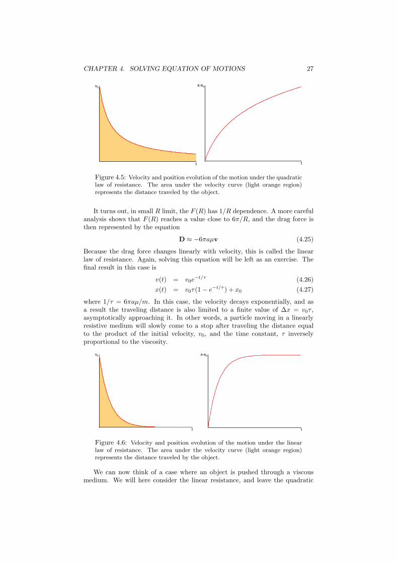
Figure 4.5: Velocity and position evolution of the motion under the quadraticlaw of resistance. The area under the velocity curve (light orange region)represents the distance traveled by the object.
It turns out, in small R limit, the F (R) has 1/R dependence. A more carefulanalysis shows that F (R) reaches a value close to 6π/R, and the drag force isthen represented by the equation
D ≈ −6πaµv (4.25)
Because the drag force changes linearly with velocity, this is called the linearlaw of resistance. Again, solving this equation will be left as an exercise. Thefinal result in this case is
v(t) = v0e−t/τ (4.26)
x(t) = v0τ(1− e−t/τ ) + x0 (4.27)
where 1/τ = 6πaµ/m. In this case, the velocity decays exponentially, and asa result the traveling distance is also limited to a finite value of ∆x = v0τ ,asymptotically approaching it. In other words, a particle moving in a linearlyresistive medium will slowly come to a stop after traveling the distance equalto the product of the initial velocity, v0, and the time constant, τ inverselyproportional to the viscosity.
v0
t
x-x0
t
Figure 4.6: Velocity and position evolution of the motion under the linearlaw of resistance. The area under the velocity curve (light orange region)represents the distance traveled by the object.
We can now think of a case where an object is pushed through a viscousmedium. We will here consider the linear resistance, and leave the quadratic

CHAPTER 4. SOLVING EQUATION OF MOTIONS 28
resistance case as an exercise. One such example is a falling object through aviscous medium such as air. The push, here, is the gravitation, and when theobject is in motion, it will experience a drag force in addition to gravity. We willset the upward direction as positive direction, so the gravitational force is thenFg = −mg. The drag force is always in the opposite direction of the directionof the motion and thus D = −mv/τ . So the equation of motion is
mdv
dt= −mg − mv
τdv
dt= −g − v
τ(4.28)
Solve the equation for initial values v0 and x0, and we get
v(t) = (v0 + gτ)e−t/τ − gτx(t) = x0 + (v0τ + gτ2)(1− e−t/τ )− gτt (4.29)
Here, the final velocity approaches v = −gτ , which is the velocity at which thenet force becomes zero, that is
Fg +D = −mg − mv
τ= 0 (4.30)
This is what is known as the terminal velocity of a motion in a drag medium.
x-x0
t
v0
t
Figure 4.7: Velocity and position evolution of the motion under a constantforce plus linear resistance. The area under the velocity curve (light greenregion subtracted from light orange region) represents the distance traveledby the object. The grey dashed line marks the point in time at which the par-ticle returns to its original position. Note that the velocity curve approachesnon-zero value due to the shift in the force equilibrium point. Accordingly,the position of the object approaches a straight line with non-zero slope repre-senting a constant velocity motion. Because the terminal velocity is negativein this case, the slope is also negative.
Suppose there is no drag force. Then the motion will indefinitely accelerate,provided that the object does not hit the wall or ground. Since there is a forceopposing the motion that grows with velocity, that acceleration has to stoponce the velocity reaches the point where the constant pushing (or pulling) ofthe object matches the drag force. At this point, there is no net force and theinertia takes over and the object continues to move at the speed of gτ . Therefore,

CHAPTER 4. SOLVING EQUATION OF MOTIONS 29
instead of asymptotically approaching zero velocity as in the no outside forcecase, the object approaches the terminal velocity. It is notable that in thiscase the velocity does not oscillate around the terminal velocity, but approachesasymptotically.
4.3.2 Harmonic oscillator
There are two types of position dependent forces that play an important role inintroductory classical mechanics. One is the gravitational force that is inverselyproportional to distance and the other is the restoring force that is responsiblefor harmonic oscillation. Such restoring force follows Hooke’s law , i.e. force isproportional to the displacement. We will take a closer inspection of them inChapter 8 and Chapter 11, respectively. For now, we will briefly look at thesimple harmonic motion in one dimension.
md2x
dt2= F = −kx
d2x
dt2+ ω2x = 0 (4.31)
where ω2 = k/m. This is a second order linear differential equation with con-stant coefficients, thus the solution should take the form x(t) = eλt. We getauxiliary equation
λ2 + ω2 = 0 (4.32)
and the general solution is then
x(t) = A1eiωt +A2e
−iωt (4.33)
where A1 and A2 are arbitrary complex numbers that should be determined bythe initial condition. By representing A1 and A2 with a set of amplitude andphase,
A1 = Ae−i(φ+π/2) and A2 = Aei(φ−π/2) (4.34)
we can rewrite the solution given by Eq. (4.33) as
x(t) = A cos(ωt− φ) (4.35)
This is an oscillatory solution, and one can easily check that the solution satisfiesthe Eq. (4.31). Here the amplitude, A, and the phase φ are two arbitraryconstants that should be determined by the initial condition. The phase φdetermines during what part of the oscillatory cycle, one’s observation begins.For example, if the initial condition is given by x0 = 0 and v0 = A0ω, theamplitude and the phase are fixed to be A = A0 and φ = π/2. Then thesolution is a simple sine function x(t) = A0 sinωt.
What is interesting about this motion is that there is a force equilibriumpoint at x = 0. Unlike the drag force case where the velocity approaches itsforce equilibrium point asymptotically, here the position oscillates around theforce equilibrium point. This is an interesting point to ponder about, and I willleave it to the readers to think about it.

Chapter 5
Lagrangian Mechanics
In essence, we have covered everything we need to know in classical mechanics,i.e. equation of motion, in the previous chapters. Most of the readers, however,would feel that most if not all of the stuff we’ve learned so far is not set apartfrom things taught in the mechanics part of the freshman physics. We can lookat some very sophisticated examples, but we will put it off to later chapters.Instead, we will develop an entirely new approach commonly known as analyticalmechanics. We will start with configuration space and generalized coordinates.
5.1 Configuration Space
Imagine applying a constant force F0 at time t = 0 on a particle with mass mat rest. It will accelerate at a constant rate a = F0/m and we can visualizethe motion in our head. Now imagine another particle with mass m attachedto a massless spring with spring constant α. The spring is compressed by somedistance A, and then being released at t = 0. The second particle will followharmonic oscillation with the oscillation frequency ω =
√α/m. This is also
not very difficult to visualize in our head. Graphical representations of thesemotions are given in Fig. 5.1.
Here, we considered two different particles moving in one dimension. How-ever, we can also represent a motion of a single particle moving in two dimen-sions with the same set of graphs. In general, each dimensional motion for eachparticle can be represented in a time-position space.
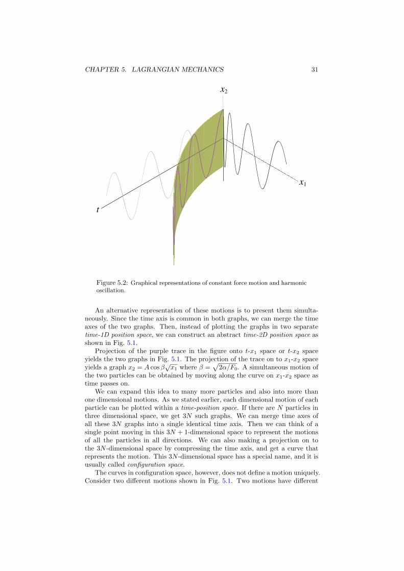
Figure 5.1: Graphical representations of constant force motion and harmonicoscillation.
30
CHAPTER 5. LAGRANGIAN MECHANICS 31
t
x1
x2
Figure 5.2: Graphical representations of constant force motion and harmonicoscillation.
An alternative representation of these motions is to present them simulta-neously. Since the time axis is common in both graphs, we can merge the timeaxes of the two graphs. Then, instead of plotting the graphs in two separatetime-1D position space, we can construct an abstract time-2D position space asshown in Fig. 5.1.
Projection of the purple trace in the figure onto t-x1 space or t-x2 spaceyields the two graphs in Fig. 5.1. The projection of the trace on to x1-x2 spaceyields a graph x2 = A cosβ
√x1 where β =
√2α/F0. A simultaneous motion of
the two particles can be obtained by moving along the curve on x1-x2 space astime passes on.
We can expand this idea to many more particles and also into more thanone dimensional motions. As we stated earlier, each dimensional motion of eachparticle can be plotted within a time-position space. If there are N particles inthree dimensional space, we get 3N such graphs. We can merge time axes ofall these 3N graphs into a single identical time axis. Then we can think of asingle point moving in this 3N + 1-dimensional space to represent the motionsof all the particles in all directions. We can also making a projection on tothe 3N -dimensional space by compressing the time axis, and get a curve thatrepresents the motion. This 3N -dimensional space has a special name, and it isusually called configuration space.
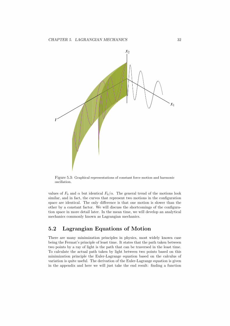
The curves in configuration space, however, does not define a motion uniquely.Consider two different motions shown in Fig. 5.1. Two motions have different
CHAPTER 5. LAGRANGIAN MECHANICS 32
t
x1
x2
Figure 5.3: Graphical representations of constant force motion and harmonicoscillation.
values of F0 and α but identical F0/α. The general trend of the motions looksimilar, and in fact, the curves that represent two motions in the configurationspace are identical. The only difference is that one motion is slower than theother by a constant factor. We will discuss the shortcomings of the configura-tion space in more detail later. In the mean time, we will develop an analyticalmechanics commonly known as Lagrangian mechanics.
5.2 Lagrangian Equations of Motion
There are many minimization principles in physics, most widely known casebeing the Fermat’s principle of least time. It states that the path taken betweentwo points by a ray of light is the path that can be traversed in the least time.To calculate the actual path taken by light between two points based on thisminimization principle the Euler-Lagrange equation based on the calculus ofvariation is quite useful. The derivation of the Euler-Lagrange equation is givenin the appendix and here we will just take the end result: finding a function
CHAPTER 5. LAGRANGIAN MECHANICS 33
x(t) that minimizes the following integral
J [x] =
∫ b
a
F (x, x, t)dt (5.1)
is equivalent to solving the following differential equation
∂F
∂x− d
dt
(∂F
∂x
)= 0 (5.2)
Now, how does this pertain to the mechanical problems that we are inter-ested? In mechanics, there is a minimization principle usually referred to asHamilton’s principle, and from this principle, we can obtain Lagrangian equa-tions of motion. Why a mechanical analysis followed from Hamiltonian principleis called Lagrangian mechanics, not Hamiltonian mechanics, may be puzzling.It is related to the historical development of Lagrangian mechanics, that is,Lagrangian mechanics in its original form did not necessarily evolve based oncalculus of variation.
Lagrange was mainly interested in developing a method that is more gen-erally applicable than Newton’s equation of motion. Naturally, the advantageof Lagrangian mechanics over Newtonian mechanics lies in the fact that it canbe used for generalized coordinate system. Another advantage is that we do notneed to know all the forces acting on the systems or particles within a system.An appropriate choice of generalized coordinates takes care of most of the im-posed constraints. This point will become more clear once we look at a fewexamples.
Hamilton’s insight that the same method can be derived from the minimiza-tion principle came later. Here, we will not follow Lagrange’s development ofLagrangian mechanics in detail. Instead, we will start with Hamilton’s principle.Hamilton’s principle in its original form states that
Of all the kinematically possible motions that take a mechanicalsystem from one given configuration to another within a given timeinterval, the actual motion is the one that minimizes the time inte-gral of the Lagrangian of the system.
In order to dissect this statement, we need to know what Lagrangian is. Wewill start by defining it, for an unconstrained one dimensional system, as thedifference between the kinetic energy, T , and potential energy, V , that is
L(x, x) = T (x, x)− V (x) (5.3)
Once the Lagrangian is defined, the Hamilton’s principle becomes,
Of all the kinematically possible motions that take a mechanicalsystem from one given configuration to another within a given timeinterval, the actual motion is the one that minimizes the integral
S[x] =
∫ t1
t0
L(x, x)dt. (5.4)

CHAPTER 5. LAGRANGIAN MECHANICS 34
By applying the Euler-Lagrangian equation(Eq. (5.2)) to minimize the aboveintegral, we get
∂L∂x− d
dt
(∂L∂x
)= 0 (5.5)
which is referred to as the Lagrange equation. With the kinetic energy andpotential energy given by
T =1
2mx2 and V = −
∫F (x)dx (5.6)
Eq. (5.5) reduces to
∂
∂x(T − V )− d
dt
[∂
∂x(T − V )
]= −dV
dt− d
dt(mx)
= F (x)−mx = 0
(5.7)
which is identical to the Newton’s equation of motion. For a system in higherdimensional space or with multiple particles, we can redefine Lagrangian bycalculating the total kinetic energy and potential energy,
T =
n∑i
Ti =
n∑i
1
2mx2
i V = V (x1, x2, · · · , xn)
L = T − V = L(x1, x2, · · · , xn, x1, x2, · · · , xn) (5.8)
One can set Euler-Lagrangian equation for each coordinate and Newtonian equa-tions of motion will be recovered. This seems like a convoluted way of reachingthe same conclusion. However, this method becomes extremely powerful in morecomplicated problems.
5.3 Generalized Coordinates
As we represent motions of N particles in three dimensional space, we needed toconstruct a configuration space of 3N -dimensions. But even if the particles areplaced in three dimensional space, sometimes their motions can be constrainedto some surfaces or lines. In such cases, appropriate coordinate transformationscan reduce the number of dimensions required to describe the motion.
Let’s first imagine an unconstrained single particle in three dimensionalspace. Using Newtonian method, we need to set up three equations of motion,one for each coordinate axis.
Fi(r) = mxi (5.9)
where the index i = 1, 2, 3 denotes three coordinate axes x, y, and z, respectively.Now we consider a particle constrained to a circle on the xy-plane. This
immediately sets two constrains to the motion
x2 + y2 = R2 and z = 0 (5.10)
where R is the radius of the ring. One can easily see that the motion is notthree dimensional, but how many dimensions should be consider? The answer,surprisingly, is one, not two. The motion certainly takes place in xy-plane which
CHAPTER 5. LAGRANGIAN MECHANICS 35
is a two dimensional surface and it seems obvious that we need two coordinatesx and y to describe the motion.
In other words, one of the constraints, z = 0, is a solution to the Eq. (5.9)with i = 3, and thus simply reduces the three dimensional problem into a twodimensional one. Now the question becomes, how should we apply the otherconstraint x2 + y2 = R2? In principle, x2 + y2 = R2 can be used to reducethe second equation of motion from Eq. (5.9) so that we are left with only oneequation to solve.
In practice, this turns out to be a near impossible task, because substitutingfor y =
√R2 − x2 and solving for Fy = my will give you a headache that
will last for days. What we want to do here is to pick a coordinate systemthat reflects the given constraints more intuitively. That coordinate system, inthis case, is the cylindrical coordinate system (3D) or polar coordinate system(2D). By setting x = r cos θ and y = r sin θ, we can replace the constraint asr = R. Then we get x = R cos θ and y = R cos θ, which are parametrized witha single variable θ. In essence, we have changed the mechanical problem of aparticle moving on a two dimensional xy-plane into a particle moving in a onedimensional θ-space.
More generally speaking, if we start with 3N dimensions and there are snumber of constraints, we need n = 3N − s dimensions to represent the motion.Depending on the nature of the constraints, the remaining dimensions are notnecessarily positions in Cartesian coordinates, or even spatial representations.As long as we can specify coordinate transformations between the 3N Carte-sian coordinates and these n new coordinates, q = (q1, q2, · · · , qn), we can takealmost anything. Such n-coordinates are referred to as the generalized coordi-nates. The number of generalized coordinates required, n, is also referred to asdegrees of freedom. Generalized coordinates have to meet two conditions:
(i) The generalized coordinates must be independent of each other, that is,there can be no functional form connecting two different coordinates.
(ii) They must fully specify the configuration of the system, that is for any givenvalues of q1, q2, · · · , qn, the position of all the N particles r1, r2, · · · , rNmust be identifiable. In other words, the position vectors of N particlesmust be known functions of the n independent generalized coordinates:
ri = ri(q1, q2, · · · , qn) (5.11)
It takes some practice to pick appropriate generalized coordinates, but agood choice of the generalized coordinates usually reflects the symmetry of themotion that we consider. In the previous example of the particle on a circularring, the circular symmetry dictates that we pick polar angle θ as the generalizedcoordinate.
However, this doesn’t help us solve Newtonian equation of motion all thatmuch better. We are still left with a problem of expressing the equation ofmotion in the generalized coordinate system, which is not trivial. This is whereLagrangian mechanics (Lagrangian equations of motion) comes in. Unlike New-tonian mechanics where the equations are based on vectors, i.e. forces, co-ordinate transformations between the 3N -dimensional configuration space andthe n-dimensional generalized configuration space are extremely cumbersome.However, because Lagrangian mechanics’ starting point is a scalar, i.e. the

CHAPTER 5. LAGRANGIAN MECHANICS 36
Lagrangian L, coordinate transformation can be implemented in a much morestraightforward manner.
5.4 Lagrangian Mechanics
With the coordinate transformations between the Cartesian coordinates andthe generalized coordinates available (see Eq. (5.11)), we can reconstruct La-grangian in the generalized coordinate system. A mechanical motion impliestime dependence in ri’s and this naturally leads to time dependence in q. Thuswe can take time derivative of q and obtain
q = (q1, q2, · · · , qn) (5.12)
which is called the generalized velocity, since it represents the velocity of thepoint q as it moves through the configuration space. One can easily derive therelationship between the real velocity of a particle and the generalized velocitythrough a simple chain rule for differentiation,
ri =∂r1
∂q1q1 + · · ·+ ∂rn
∂qnqn (5.13)
and kinetic energy of the total system, in terms of the generalized velocity,becomes
T =
n∑j
n∑k
ajk(q)qj qk (5.14)
where
ajk(q) =1
2
N∑i
mi
(∂ri∂qj· ∂ri∂qk
)(5.15)
The kinetic energy T is then a function of q = (q1, · · · , qn) and q = (q1, · · · , qn).Similarly, the potential energy V can be rewritten as a function of q. Then theLagrangian becomes a function of the generalized coordinates and generalizedvelocities:
L = L(q1, · · · , qn, q1, · · · , qn) (5.16)
In applying Hamilton’s principle to mechanics, there is no reason to believethat it should work in real coordinates only. In other words, we can apply thecalculus of variations using Lagrangian expressed in the generalized coordinates,and we are then left with n number of Lagrange equations to solve
∂L∂qj− d
dt
(∂L∂qj
)= 0 (5.17)
where i = 1, 2, · · · , n.By rewriting the equation
d
dt
(∂T
∂qj
)− ∂T
∂qj= −∂V
∂qj= Qj (5.18)
we can see that there is a term, Qj , that is defined in the generalized coordinate,corresponding to the concept of force in the real space. For this reason, Qj is
CHAPTER 5. LAGRANGIAN MECHANICS 37
known as the generalized force. By applying the chain rule in calculating thisderivative of potential with respect to the generalized coordinates, it is easy toprove that the generalized force and the real space force has the relationship:
Qj =∑i
Fi ·∂ri∂qj
(5.19)
where Fi is the specified force acting on the i-th particle.So far, we have only considered a constraint that can be expressed in the form
of ri = ri(q). Such constraints are referred to as geometric constraints, becausethe coordinate transformation between the real coordinates and generalized co-ordinates is purely geometric, that is there is no explicit time dependence orvelocity dependence in the coordinate transformation. Such a system is said tobe holonomic. Establishing Lagrangian mechanics for a non-holonomic systemin general is outside the scope of this course and we will not treat the problemhere.
However, time dependent constraint can be relatively easily integrated intothe Lagrange equations. Also, there are some cases where the generalized forcecan be expressed in the form
Qj =d
dt
(∂V
∂qj
)− ∂V
∂qj(5.20)
for some function V (q, q, t). Then the function V (q, q, t) is called the velocitydependent potential of the system and Lagrangian is given by
L(q, q, t) = T (q, q, t)− V (q, q, t) (5.21)
and one can still use Lagrange equation to solve mechanics problems. Notethat the velocity dependent potential produces non-conservative force as theresulting force is not strictly position dependent.
5.5 D’Alembert’s Principle
It seems pretty obvious, by now, that with the help of Hamilton’s principle andthe definition of Lagrangian L(q, q, t) = T (q, q, t) − V (q, q, t), one can easilycome up with a mechanical equation in generalized coordinates whose solutioncan be transformed later into a real space solution. However, there is a naggingquestion regarding the definition of Lagrangian, that is ”how did someone comeup with such a physical quantity that produces the Lagrangian equation?” Theanswer to this question lies, as stated earlier, in the fact that the Hamilton’sprinciple came after Lagrange came up with his definition of Lagrangian. ForLagrange, the starting point was virtual work and D’Alembert’s principle.
Suppose a system with N particles where an individual particle is subjectto a net force,
Fi = FSi + FCi = mivi (5.22)
where FSi denotes the specified force and FCi denotes the constraint force. Inother words, we know explicitly how the FSi ’s act on each particle, but theeffect of FCi ’s is not known to us, except for the fact that the constraint forceacts as a boundary condition. For most cases, the direction of such constraints
CHAPTER 5. LAGRANGIAN MECHANICS 38
are orthogonal to the directions of particle’s allowed motion. The effect of theconstraint can be thus written as
N∑i
FCi · vi = 0 (5.23)
In other words, we can rewrite the equation of motion for the total system as
N∑i
mivi · vi =
N∑i
FSi · vi +
N∑i
FCi · vi =
N∑i
FSi · vi (5.24)
where the constraint force is no longer explicit.However, one can consider a virtual path that is also subject to the same
constraint force, and by denoting the velocity along that virtual path as v∗i , wecan get the identical relation
N∑i
mivi · v∗i =
N∑i
FSi · v∗i (5.25)
which is known as the D’Alembert’s principle.For a holonomic system with constraint force doing no virtual work, there
must be a generalized coordinate system q that links the real space positionof the particles ri’s to q. With such generalized coordinate system, we canconstruct a virtual motion v∗i
v∗i =∂r
∂q1(5.26)
that corresponds to the motion generated by generalized velocities
q1 = 1, q2 = 0, · · · , qn = 0 (5.27)
From d’Alembert’s principle, we get
N∑i
mivi ·∂ri∂q1
=
N∑i
FSi ·∂ri∂q1
(5.28)
We can consider different virtual motion generated by q1 = q2 = · · · = qn = 0for all the generalized coordinates except for qj = 1. For all the possible valuesof j, we get n equations
N∑i
mivi ·∂ri∂qj
=
N∑i
FSi ·∂ri∂qj
(5.29)
The left hand side of the equation can be rewritten in terms of qj ’s
N∑i
mivi ·∂ri∂qj
=d
dt
(∂T
∂qj
)− ∂T
∂qj=
N∑i
FSi ·∂ri∂qj
(5.30)
which is identical to the Lagrange equation given by Eq. (5.18). Now one canwork backwards what we treated in the previous sections and define Lagrangianas T − V and also come up with Hamilton’s principle.
CHAPTER 5. LAGRANGIAN MECHANICS 39
5.6 Conjugate Variables
Up to this point, we have treated how an appropriate choice of generalizedcoordinates can simplify solving mechanical problems. According to such choice,we have constructed generalized velocities and generalized forces. It is onlynatural to suspect that there must be generalized momenta. In Lagrangianmechanics, the generalized momentum corresponding to the coordinate qi isdefined as
pi ≡∂L∂qi
(5.31)
It is also called the momentum conjugate to qi. In this case, the generalized co-ordinate and the generalized momentum are said to be conjugate variables. TheLagrangian equation can be rewritten in terms of the generalized momentum
∂L∂qi
= pi (5.32)
From this, one can easily see that the generalized momentum, pi, is conservedif the corresponding coordinate, qi is cyclic, i.e. absent from the Lagrangian.
In general, the Lagrangian is a function of q, q and t. The case where qi isabsent from Lagrangian is a special case of qi being cyclic with zero generalizedmomentum. An interesting point here to consider is what happens if the timet is cyclic? Is there a conjugate momentum to time? To answer this question,we will move on to the next topic, the Hamiltonian mechanics.
Chapter 6
Hamiltonian Mechanics
We now turn our attention to Hamilton’s formalization of mechanics. It shouldbe made clear from the very beginning that in terms of solving problems inclassical mechanics, Hamiltonian mechanics provides almost no advantage overLagrangian mechanics. In fact, in most cases, things appear to be more difficultto solve with Hamiltonian mechanics. The benefits of Hamiltonian mechanicslie in interpretation of mechanical motion and as a bridge towards statisticalmechanics and quantum mechanics.
6.1 Legendre Transformation: From Lagrangianto Hamiltonian
In the previous chapter, we defined generalized momentum pi as the conjugatemomentum of the generalized coordinate, qi, as
pj =∂
∂qjL(q, q, t) (6.1)
and this yields the Lagrangian equation of motion into the following form
pj =∂
∂qjL(q, q, t). (6.2)
Here we have a differential equation for pj expressed in terms of variables q,q and t. To have a self-consistent form of the differential equation, it wouldbe desirable to formulate the equation in terms of p instead of q. This canbe achieved by performing a functional transformation known as the Legen-dre transformation. For anyone that is interested in the mathematics of thederivation, detailed calculation is given in the appendix. By performing thetransformation, we can construct a function H(q,p, t) as below
H(q,p, t) = q · p− L(q, q, t). (6.3)
Here, the variables that do not participate in transformation, i.e. q and t, arereferred to as passive variables, and naturally the variables that do participatein transformation, i.e. q and p, are called the active variable.
40

CHAPTER 6. HAMILTONIAN MECHANICS 41
At first glance, it is not obvious that the new function H is a function of q,p and t. Rather, it seems like a function of all four variables q, q, t and p. Tosee this, we will take a differential of H:
dH =
n∑i=1
(qidpi + pidqi)−n∑i=1
∂L∂qi
dqi −n∑i=1
∂L∂qi
dqi −∂L∂tdt
=
n∑i=1
qidpi +
n∑i=1
(pi −
∂L∂qi
)dqi −
n∑i=1
∂L∂qi
dqi −∂L∂tdt
(6.4)
From the definition of the generalized momentum, the second term in the secondline of the above equation is zero, that is, the differential of H does not containany term with dq. In other words, the function H is not a function of qs, butonly of q, p and t. This function, H, is called the Hamiltonian function or justHamiltonian.
6.2 Hamilton’s Equations
For two functions H(q, q, t) and H(q,p, t) that are Legendre transformation ofeach other, following relations hold:
∂L∂qj
= −∂H∂qj
(6.5)
pj =∂L∂qj
(6.6)
qj =∂H∂pj
(6.7)
with p being a passive variable and q and p as active variables. Again proof ofthese relations are presented in appendix and we will simply use this relationhere. Combining Eq. 6.5 and Eq. 6.6 with Lagrangian equation of motion,Eq. 5.17, we can show that
pj =d
dt
(∂L∂qj
)=∂L∂qj
= −∂H∂qj
(6.8)
Inspecting Eq. 6.7 and Eq. 6.8, one can see that they form a set of 2n first orderdifferential equations that specifies all the relationship required to solve for qand p. These are the Hamiltonian equations of motion or simply Hamilton’sequations:
qj =∂H∂pj
pj = −∂H∂qj
(6.9)
In other words, we have just swapped out Lagrange equations, which are nsecond order differential equations, with Hamilton’s equation, 2n first orderdifferential equations.
Note that there is a nice symmetry to the equations. It will become moreobvious with a different notation for the variables, ξk:
ξk =
qk for k = 1, 2, · · · , npk−n for k = n+ 1, · · · , 2n (6.10)

CHAPTER 6. HAMILTONIAN MECHANICS 42
Then the Hamilton’s equations become
ξk =∂H(ξ, t)
∂ξk+nfor k = 1, 2, · · · , n
ξk = −∂H(ξ, t)
∂ξk−nfor k = n+ 1, · · · , 2n
(6.11)
Since the RHS of the above equations result in some functions of ξ = (ξ1, ξ2, · · · , ξ2n)and t, for all values of k running from 1 to 2n, the equations can be rewrittenas:
ξk = fk(ξ1, ξ2, · · · , ξ2n, t) (6.12)
In this regard, the generalized coordinates q and the generalized momentump are indistinguishable. In other words, qjs and pjs are independent variablesthat are on equal footings.
Aside from the beautiful simplicity in expressing the equations of motionas Eq. 6.12, it is not obvious at all why one would formulate the equations inthis way. As a matter of fact, unless the Hamiltonian is given a priori, theprocess described above is not any less painful than the Lagrangian mechanics.Setting up Hamilton’s equations of motion requires constructing Hamiltonianfrom Lagrangian, and there is a step that makes finding Hamilton’s equationsfrom Hamiltonian practically meaningless.
To illustrate this point, we turn to our favorite example once again, onedimensional simple harmonic oscillator. We start from the Lagrangian
L =1
2mx2 − 1
2kx2 (6.13)
and the generalized momentum is then
p =∂L∂x
= mx (6.14)
The velocity, x, is then expressed in terms of the momentum, p,
x =p
m(6.15)
and this lets us formulate Hamiltonian
H = px− L =p2
2m+
1
2kx2. (6.16)
Hamiltonian has to be expressed in terms of q, p and t only, and the generalizedvelocity q must be expressed as a function of the generalized momentum p. Thisis done, in the above example, by converting Eq. 6.14 into Eq. 6.15 and thenEq. 6.15 being plugged into Eq. 6.16. Once the Hamiltonian is obtained, we canfind the Hamilton’s equations:
x =∂H∂p
=p
m(6.17)
p = −∂H∂x
= −kx (6.18)
However, notice that the first of the two equations, Eq. 6.17, is nothing butEq. 6.15. The fact that two equations, Eq. 6.15 and Eq. 6.17, are identical is

CHAPTER 6. HAMILTONIAN MECHANICS 43
no surprise, as it is a salient feature of Legendre transformation. However, apart of the Hamilton’s equations are produced in the process of constructingHamiltonian makes the whole process somewhat circular.
An attempt to solve the Hamilton’s equations, Eq. 6.17 and Eq. 6.18, inflictsmore disappointment. Because two Hamilton’s equations are coupled, that is xis a function of p and p is a function of x, to solve these equations, one ends updifferentiating Eq. 6.17 with respect to time and plugging it into Eq. 6.18. Theend result yields
x+k
mx = 0 (6.19)
which is identical to the Lagrangian equation (and Newtonian equation). Sowhat is the point of all this practice other than causing you a massive headache?To find (one of) the answer(s), we’ll take a trip into the phase space.
6.3 Configuration Space and Phase Space
In formulating the Lagrangian mechanics, we emphasized the importance offinding n independent generalized coordinates, q = (q1, q2, · · · , qn) formingthe configuration space. The Lagrange equation yields time dependent solu-tions for the qj(t)’s. Since we can trace out the motions of a mechanical sys-tem of interest in real space with an appropriate coordinate transformations,ri(t) = ri(q1(t), q2(t), · · · , qn(t)), for all N particles, any mechanical motion canbe represented by a point q(t) = (q1(t), q2(t), · · · , qn(t)) moving through theconfiguration space.
As powerful as this method seems, this is not an effective method of visuallyrepresenting a mechanical motion, as this involves time evolution of a pointalong the phase space. We have seen in the previous chapter that a trajectoryin the configuration space, that is a graphical representation of the motionobtained by compressing the time evolution and projecting all the motion on tothe configuration space, is not a unique identification of motion.
It is quite obvious why this is so. The Lagrangian equations of motion aresecond order differential equations. To exactly solve a second order differentialequation, we need two initial conditions, not one to obtain the exact solution.In Newtonian mechanics, these two initial conditions were the position andvelocity. A point in configuration space specifies the initial positions but notinitial velocities.
This shortcoming is averted in the Hamiltonian formulation as the mechan-ical motion is represented in a 2n-dimensional space spanned by both q andp. As we said in the previous section, in Hamiltonian mechanics, q and p areindependent variables that need to be solved from the 2n first order differentialequations simultaneously. Therefore, at any given moment, the solution to theequation is expressed as q(t) and p(t). A graphical representation, thus requiresa point in q-p space, a 2n-dimensional vector space also known as the phasespace.
The phase space by nature is 2n-dimensional and identifying any point insidethe phase at a given moment provides us with 2n initial conditions. Therefore, atrajectory in phase space has no ambiguity unlike that of a configuration space.
To make this point clear, let us look at an example of simple harmonicoscillators in one dimension. Imagine pulling on a particle with mass m attached
CHAPTER 6. HAMILTONIAN MECHANICS 44
to a spring with spring constant α. We pull the particle by a displacement of A,hold it still and then let go of it. Here, there is only one generalized coordinate x,which is identical to the real coordinate of the particle. Thus the configurationspace is simply one dimensional space represented by x. A trajectory in theconfiguration space is a line between x = −A and x = A as shown in Fig. ??.
Let’s consider another particle with mass m attached to a spring with springconstant 4α this time. If the initial displacement is again x = A, the trajectoryin the configuration space is identical to the one from above (See Fig. ??).Put differently, without the explicit time evolution along the trajectory, thetrajectory itself does not allow us to identify the motion in configuration space.
We will now look at these two cases in the phase space. For the first case withspring constant of α, any loss of potential energy, α(A2 − x2)/2, is convertedinto kinetic energy, p2/2m, and thus we have the relation
1
2αx2 +
p2
2m=
1
2αA2 (6.20)
This is an equation of ellipse in the x-p phase space (See Fig. ??). The secondspring with four times as big spring constant yields the phase space trajectoryalong
2αx2 +p2
2m= 2αA2 (6.21)
which is a totally different ellipse than the first one. When trajectories such asthese ellipses are presented in the phase space, each of them uniquely definesthe motion and any time evolution of a point on the trajectory can be exactlyestimated.
However, there is another subtle but possibly more important point in phasespace. For a given set of equations of motion, there is only one trajectory thatpasses through any given point in the phase space. In other words, trajectoriesin phase space do not overlap or cross one another. This is equivalent to sayingthat when the initial conditions are fully specified, there is one and only oneexact solution to the equations of motion.
We will take an example of a particle with mass m that can move onlyin one dimension, say x-axis. The particle is under a constant force F alongthe positive x direction. The general solution to this problem in Hamiltonianmechanics is
x(t) =1
2
F
mt2 +
p0
mt+ x0 (6.22)
where x0 and p0 are initial position and momentum of this particle, respectively.The proof of this is left for the readers. Also, from the Hamilton’s equations,one can easily show that
p(t) = p0 + Ft (6.23)
Combining the two solutions, we have the phase space trajectory:
x =p2
2mF− p2
0
2mF+ x0 (6.24)
which gives us an infinite set of parabolas depending on the values of x0 and p0,a few of which are drawn in Fig. ??. The key feature here is that for any pointinside the phase space, there is only one trajectory that passes through thatpoint. The point is permanently attached to that trajectory and flows along itin a specific direction.
CHAPTER 6. HAMILTONIAN MECHANICS 45
6.4 Hamiltonian and Energy
To figure out another important aspect of Hamiltonian mechanics, let us take atime derivative of the Lagrangian in its most general form:
d
dtL(q, q, t) =
n∑i=1
(∂L∂qi
qi +∂L∂qi
qi
)+∂L∂t
(6.25)
By now, you should be able to identify immediately that
∂L∂qi
= pi∂L∂qi
= pi (6.26)
and Eq. 6.25 becomes
dLdt
=
n∑i=1
(piqi + piqi) +∂L∂t
=d
dt
(n∑i=1
piqi
)+∂L∂t
(6.27)
From this, we can see that the time derivative of the Lagrangian is generally notconstant even if the Lagrangian has no explicit time dependence, i.e. ∂L
∂t = 0.From Eq. 6.3, we can see that the first term in the RHS of the above equationis L+H:
dLdt
=d
dt(L+H) +
∂L∂t. (6.28)
Therefore, we havedHdt
= −∂L∂t. (6.29)
that is, if the Lagrangian is not an explicit function time, the Hamiltonianis conserved. A fancy way of saying is that if the system is time-translationinvariant, then the Hamiltonian is conserved. Going back to the last questionwe had at the end of the previous chapter, we can see that the Hamiltonian isthe conjugate momentum of time.
In fact, it is quite straightforward to show that, for very simple conserva-tive systems such as a harmonic oscillator, or a particle under the influence ofa constant force, that the Hamiltonian is sum of the kinetic energy and thepotential energy, i.e. total mechanical energy. We leave it as an exercise forreaders. However, the Hamiltonian is a more general form of energy that thetotal mechanical energy given by E = T + V and on this ground, we equateHamiltonian with the total energy of the system.
The identification of Hamiltonian as the total energy allows us to approachmechanics of conservative system without actually solving the equation of mo-tion. We go back to the single particle under constant force in one dimension.Since the force is constant throughout space, the system is conservative. Thuswe can write down the Hamiltonian as
H = T + V =p2
2m− Fx = constant(E). (6.30)
If we solve the above equation for x, we get
x =p2
2mF− E
F. (6.31)
CHAPTER 6. HAMILTONIAN MECHANICS 46
One can immediately notice the similarity between the above equation and theEq. 6.24. Upon a close inspection, we can see that they are, in fact, identical.For the given initial position and momentum of x0 and p0, the total energy of
the system is E =p202m − Fx0, and substituting this for E in Eq. 6.31, we get
exactly the same equation as Eq. 6.24.This raises two interesting points for the case where the Lagrangian has no
explicit time dependence. First is that the Hamiltonian also has no explicittime dependence, and we have H(q,p) = E. This is an equation for a (2n− 1)-dimensional surface in the 2n-dimensional phase space. We can therefore obtainthe surface along which the motion takes place in the phase space without havingto solve any differential equations. Exact time evolution is not immediatelyaccessible, but a geometrical solution in the phase space is directly handed tous.
The second point is that the two initial conditions x0 and p0 are rolledup in the total energy E. This is a combined effect of uniqueness of phasespace trajectory (or surface) and time-translation invariance. As we emphasizedearlier, for any given initial condition, the phase space trajectory is unique anda point in phase space cannot escape from that trajectory. Also, the geometricsolution, i.e. the trajectory or surface, in the phase space is not time stamped,and it represents the entire history of the motion from negative infinite time topositive infinite time. If the system has time-translation invariance, that is, ifthe system is unaffected by sliding up and down along the time axis, it meanswe can slide identification of certain position, x0, and momentum, p0, at a givenmoment, t0, loses its meaning. Without actually following the time evolution,we can slide in time from t0 to t0 + ∆t by an arbitrary amount ∆t and set thatmoment as our initial moment. It will shift the initial conditions to x0 +∆x andp0 + ∆p, yet remains on the same trajectory on the phase space. Thus, the onlything that is relevant in identifying the solution is the phase space trajectorydetermined by the total energy E and not the initial conditions x0 and p0.

Chapter 7
Central Force Motion
From the historical point, central force motion is one of the most importantproblems in classical mechanics. It was people’s desire to understand planetarymotions and stellar objects that gave rise to much of Newton’s finest works, andit turns out that the planets and stellar objects are governed by gravity, oneof the two most representative cases of the central forces, along with Coulombforce in electrodynamics.
Central force is a force with spherical symmetry that only depends on thedistance from the center of the force field. In other words, a force field F(r) issaid to be a central force field with center O if it has the form
F(r) = F (r)r (7.1)
where r = |r| and r = r/r. Gravity falls in this category as the force betweentwo massive objects with masses m and M is given by the relation
F (r) = −GmMr2
(7.2)
Note that central force is a function of position and thus is a conservative forcewith potential, V (r), satisfying
F (r) = −dV (r)
dr(7.3)
Also, due to the symmetry of the force field, an object’s motion under centralforce field is always planar, that is, the object is bound in a plane formed bythe center of the force field, the position and the velocity vector of the objectunder the influence of the central force. Thus two dimensional polar coordinateis sufficient to describe the motion in its full detail. In the following sections,we have performed all the calculations with the mass of object included. Notethat in the textbook by Gregory, they have performed all the calculations forunit mass. We leave it to you to try and convert the equations between twodifferent forms. It is something you should be able to do.
7.1 Conservation Laws in Central Force Field
The central force conserves the system’s angular momentum. This is becausethere is no net torque acting on the particle as the force is always along the
47
CHAPTER 7. CENTRAL FORCE MOTION 48
direction of the moment arm,
K = r× F = F (r)r× r = 0 (7.4)
This can be also seen from the Lagrangian
L = T − V =1
2m(r2 + r2θ2
)− V (r) (7.5)
which is cyclic about θ, and the angular momentum pθ is conserved,
pθ =∂L
∂θ= mr2θ = constant = l (7.6)
The angular momentum conservation can be rewritten as
θ =l
mr2(7.7)
θ(t) =
∫ t
0
l
m[r(τ)]2dτ, (7.8)
which means that once the time dependence of r(t) is known, the time depen-dence of θ(t) can be easily found out.
The second Lagrange equation is
F (r) +mrθ2 −mr = F (r) +l2
mr3−mr = 0 (7.9)
This is an ordinary differential equation for the radial distance r(t) which isgenerally not solvable.
Instead of solving the differential equation, we can obtain qualitatively de-scription of the motion based on another feature of the Lagrangian. The La-grangian is not an explicit function of t, and thus the energy function h mustbe conserved.
h = r∂L
∂r+ θ
∂L
∂θ− L =
1
2m(r2 + r2θ2
)+ V (r) = constant = E (7.10)
Using Eq. (7.7), we can rewrite the above equation as
1
2mr2 + V (r) +
l2
2mr2= E (7.11)
In fact, this is identical to Eq. (7.9) as taking the time derivative of the aboveequation yields Eq. (7.9). One important feature of the above equation is thatthe angular velocity component of the kinetic energy is reformulated as a func-tion of r,
1
2mr2θ2 =
l2
2mr2(7.12)
and this allows us to define the effective potential
Veff (x) = V (x) +l2
2mx2(7.13)
We can then treat the system as a one dimensional particle moving with kineticenergy T = 1
2mx2 under the potential energy Veff (x):
1
2mx2 + Veff(x) = E (7.14)
with x > 0. Even if we cannot solve the equation exactly, one can easily definethe range of motion in r by plotting the effective potential Veff(x) and E.

CHAPTER 7. CENTRAL FORCE MOTION 49
7.2 The Path Equation
Solving the Eqs. (7.8) and (7.9) can give us a full picture of the time dependentmotion. However, with r(t) and θ(t) given, we can use them to get parametricequation r(θ), which is typically dubbed the orbit of the system.
Instead of having to find r(t) and θ(t) to find the orbit, one can combineEq. (7.9) and (7.7) to eliminate time. By introducing a new variable u = 1/r,
r = − l2u2
m2
d2u
dθ2(7.15)
rθ2 =l2u3
m2(7.16)
and we can rewrite Eq. (7.9) as
d2u
dθ2+ u+
mF (1/u)
l2u2= 0 (7.17)
This is the path equation. Only for inverse square law and inverse cube laws,the path equation becomes a linear equation. Otherwise, this is a non-linearequation. It is rather fortunate that the gravity is an inverse square law, whichcan be solved analytically.
We will, in fact, take a look at the attractive inverse square law whereF (r) = −γ/r2 = −γu2. Then the path equation is a linear equation of the form
d2u
dθ2+ u− mγ
l2= 0 (7.18)
The general solution of the equation is
1
r= A cos(θ − α) +
mγ
l2=mγ
l2(1 + e cos(θ − α)) (7.19)
Since we are interested in the path of orbital motion, we can set α to be zeroand, without losing generality, rewrite the equation
1
r=mγ
l2(1 + e cos θ) (7.20)
The eccentricity e = Al2
mγ is related to the initial condition and if e = 0, the pathis a circle. If e < 1, then the path is an ellipse. For e = 1 and e > 1, the resultsare parabola and hyperbola respectively.
Also, by comparing the Eq. (7.20) to the standard polar equation of a conic
1
r=
a
b2(1 + e cos θ) (7.21)
we get the relation between the angular momentum l and the conic parametersa and b,
l2 = mγb2
a(7.22)
This relation is known as the L-formula. The total energy E and the conicparameter a can be also shown to have the following relation, E-formula
Ellipse : E = − γ2a < 0
Parabola : E = 0Hyperbola : E = γ
2a > 0(7.23)

CHAPTER 7. CENTRAL FORCE MOTION 50
For a particle moving under the central force field obeying the repulsiveinverse square law, the force is given by F (r) = γ/r2, and the path equation iscorrespondingly,
d2u
dθ2+ u+
mγ
l2= 0 (7.24)
whose solution can only be a parabola or hyperbola,
1
r=mγ
l2(−1 + e cos θ) . (7.25)
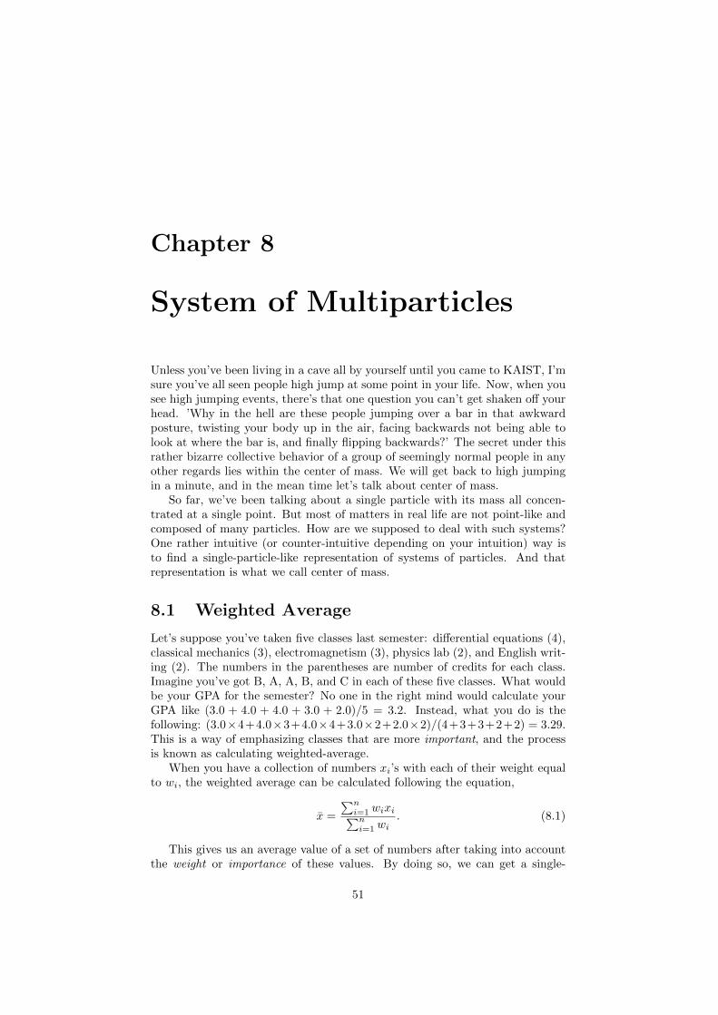
Chapter 8
System of Multiparticles
Unless you’ve been living in a cave all by yourself until you came to KAIST, I’msure you’ve all seen people high jump at some point in your life. Now, when yousee high jumping events, there’s that one question you can’t get shaken off yourhead. ’Why in the hell are these people jumping over a bar in that awkwardposture, twisting your body up in the air, facing backwards not being able tolook at where the bar is, and finally flipping backwards?’ The secret under thisrather bizarre collective behavior of a group of seemingly normal people in anyother regards lies within the center of mass. We will get back to high jumpingin a minute, and in the mean time let’s talk about center of mass.
So far, we’ve been talking about a single particle with its mass all concen-trated at a single point. But most of matters in real life are not point-like andcomposed of many particles. How are we supposed to deal with such systems?One rather intuitive (or counter-intuitive depending on your intuition) way isto find a single-particle-like representation of systems of particles. And thatrepresentation is what we call center of mass.
8.1 Weighted Average
Let’s suppose you’ve taken five classes last semester: differential equations (4),classical mechanics (3), electromagnetism (3), physics lab (2), and English writ-ing (2). The numbers in the parentheses are number of credits for each class.Imagine you’ve got B, A, A, B, and C in each of these five classes. What wouldbe your GPA for the semester? No one in the right mind would calculate yourGPA like (3.0 + 4.0 + 4.0 + 3.0 + 2.0)/5 = 3.2. Instead, what you do is thefollowing: (3.0×4+4.0×3+4.0×4+3.0×2+2.0×2)/(4+3+3+2+2) = 3.29.This is a way of emphasizing classes that are more important, and the processis known as calculating weighted-average.
When you have a collection of numbers xi’s with each of their weight equalto wi, the weighted average can be calculated following the equation,
x =
∑ni=1 wixi∑ni=1 wi
. (8.1)
This gives us an average value of a set of numbers after taking into accountthe weight or importance of these values. By doing so, we can get a single-
51
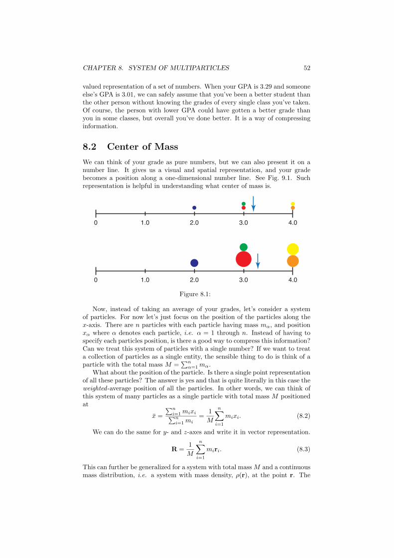
CHAPTER 8. SYSTEM OF MULTIPARTICLES 52
valued representation of a set of numbers. When your GPA is 3.29 and someoneelse’s GPA is 3.01, we can safely assume that you’ve been a better student thanthe other person without knowing the grades of every single class you’ve taken.Of course, the person with lower GPA could have gotten a better grade thanyou in some classes, but overall you’ve done better. It is a way of compressinginformation.
8.2 Center of Mass
We can think of your grade as pure numbers, but we can also present it on anumber line. It gives us a visual and spatial representation, and your gradebecomes a position along a one-dimensional number line. See Fig. 9.1. Suchrepresentation is helpful in understanding what center of mass is.
0 4.02.0 3.01.0
0 4.02.0 3.01.0
Figure 8.1:
Now, instead of taking an average of your grades, let’s consider a systemof particles. For now let’s just focus on the position of the particles along thex-axis. There are n particles with each particle having mass mα, and positionxα where α denotes each particle, i.e. α = 1 through n. Instead of having tospecify each particles position, is there a good way to compress this information?Can we treat this system of particles with a single number? If we want to treata collection of particles as a single entity, the sensible thing to do is think of aparticle with the total mass M =
∑nα=1mα.
What about the position of the particle. Is there a single point representationof all these particles? The answer is yes and that is quite literally in this case theweighted -average position of all the particles. In other words, we can think ofthis system of many particles as a single particle with total mass M positionedat
x =
∑ni=1mixi∑ni=1mi
=1
M
n∑i=1
mixi. (8.2)
We can do the same for y- and z-axes and write it in vector representation.
R =1
M
n∑i=1
miri. (8.3)
This can further be generalized for a system with total mass M and a continuousmass distribution, i.e. a system with mass density, ρ(r), at the point r. The

CHAPTER 8. SYSTEM OF MULTIPARTICLES 53
summation then becomes an integral and the center of mass is
R =
∫ρ(r)rdV∫ρ(r)dV
=1
M
∫ρ(r) r dV. (8.4)
We have thus far calculated the center of mass. Now the natural question thatfollows is ”how is this useful”? We will deal with this question in the next fewfollowing sections.
8.3 Linear Momentum
Let’s first think about the linear momentum of a system of particles. Eachparticle in the system would have its own momentum, and we will denote themomentum of the i-th particle as pi = miri. If we are to calculate the totalmomentum of the system with all n-particles in it, we can just sum over i andwe get
P =∑i
pi =∑i
miri =d
dt
∑i
miri =d
dtMR = MR, (8.5)
which is to say:I. The linear momentum of the system is the same as if a single particle of massM were located at the position of the center of mass and moving in the mannerthe center of mass moves.
What about the time derivative of the momentum? Before we answer thisquestion, let’s actually impose a couple of assumptions. When we have a col-lection of particles, it is entirely possible that there is some type of force actingon one particle by another. For example, if we have a bunch of electrons, therewill be Coulomb force acting between each pair of electrons. This is what wecall internal force and we will assume the following about the internal force:
The internal force acting on a particle i by another particle j is equalin size and opposite in direction to the force acting on the particle jby the particle i. That is Gij = −Gji, where Gij denotes the forceacting on i by j. This is in fact Newton’s Third Law.
With these assumptions in mind, we now turn to external force. It is con-ceivable that there is a force acting on a particle that is not exerted by otherparticles that constitute the system. Any force acting on a particle i that is notcoming from within the system is what we call external force. We will denotethe external force as Fi. In such a case, the total amount of force acting onthe particle i, Fnet
i is Fneti = Fi +
∑j Gij . Here, the internal force on the i-th
particle,∑j Gij , is summed over all the other particles j 6= i’s in the system.
(Alternatively, we can set the internal force coming from the particle itself isnull, i.e. Gii = 0. The equation of motion for the i-th particle is Fnet
i = miri,and by summing over i we get the equation of motion for the total system,
F =∑i
Fneti =
∑α
Fi +∑i
∑j 6=i
Gij =∑α
Fi +∑i
∑j<i
(Gij + Gji)(8.6)
=∑i
miri =d2
dt2
∑i
miri =d2
dt2MR = MR = P (8.7)
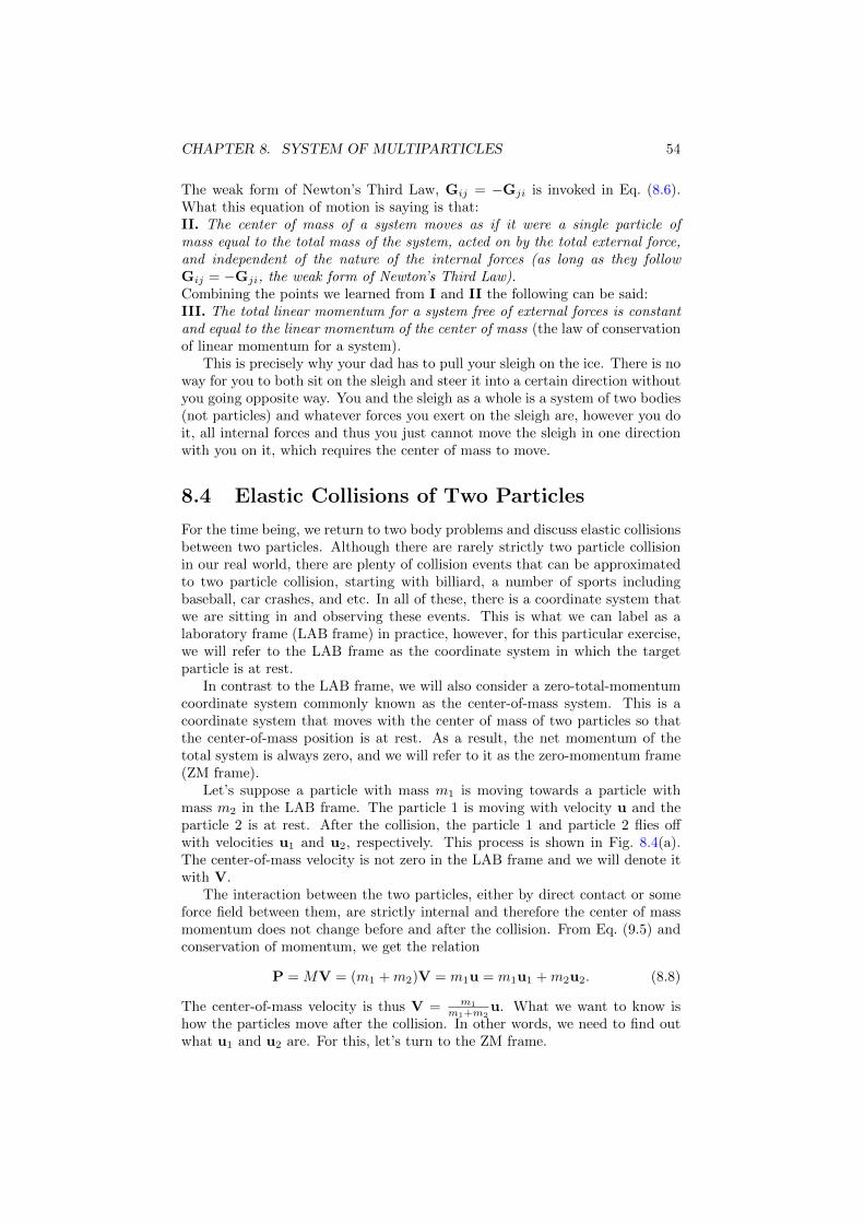
CHAPTER 8. SYSTEM OF MULTIPARTICLES 54
The weak form of Newton’s Third Law, Gij = −Gji is invoked in Eq. (8.6).What this equation of motion is saying is that:II. The center of mass of a system moves as if it were a single particle ofmass equal to the total mass of the system, acted on by the total external force,and independent of the nature of the internal forces (as long as they followGij = −Gji, the weak form of Newton’s Third Law).Combining the points we learned from I and II the following can be said:III. The total linear momentum for a system free of external forces is constantand equal to the linear momentum of the center of mass (the law of conservationof linear momentum for a system).
This is precisely why your dad has to pull your sleigh on the ice. There is noway for you to both sit on the sleigh and steer it into a certain direction withoutyou going opposite way. You and the sleigh as a whole is a system of two bodies(not particles) and whatever forces you exert on the sleigh are, however you doit, all internal forces and thus you just cannot move the sleigh in one directionwith you on it, which requires the center of mass to move.
8.4 Elastic Collisions of Two Particles
For the time being, we return to two body problems and discuss elastic collisionsbetween two particles. Although there are rarely strictly two particle collisionin our real world, there are plenty of collision events that can be approximatedto two particle collision, starting with billiard, a number of sports includingbaseball, car crashes, and etc. In all of these, there is a coordinate system thatwe are sitting in and observing these events. This is what we can label as alaboratory frame (LAB frame) in practice, however, for this particular exercise,we will refer to the LAB frame as the coordinate system in which the targetparticle is at rest.
In contrast to the LAB frame, we will also consider a zero-total-momentumcoordinate system commonly known as the center-of-mass system. This is acoordinate system that moves with the center of mass of two particles so thatthe center-of-mass position is at rest. As a result, the net momentum of thetotal system is always zero, and we will refer to it as the zero-momentum frame(ZM frame).
Let’s suppose a particle with mass m1 is moving towards a particle withmass m2 in the LAB frame. The particle 1 is moving with velocity u and theparticle 2 is at rest. After the collision, the particle 1 and particle 2 flies offwith velocities u1 and u2, respectively. This process is shown in Fig. 8.4(a).The center-of-mass velocity is not zero in the LAB frame and we will denote itwith V.
The interaction between the two particles, either by direct contact or someforce field between them, are strictly internal and therefore the center of massmomentum does not change before and after the collision. From Eq. (9.5) andconservation of momentum, we get the relation
P = MV = (m1 +m2)V = m1u = m1u1 +m2u2. (8.8)
The center-of-mass velocity is thus V = m1
m1+m2u. What we want to know is
how the particles move after the collision. In other words, we need to find outwhat u1 and u2 are. For this, let’s turn to the ZM frame.
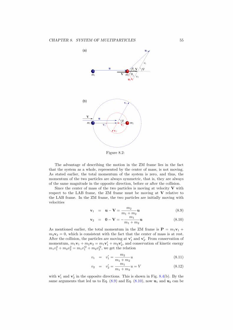
CHAPTER 8. SYSTEM OF MULTIPARTICLES 55
u
u1
V
u2
V
m1 m2
ψθ1
θ2
v1’ v2’m1 m2
v1
v2
uV
ψ
(a)
(b)
v1
v2
Figure 8.2:
The advantage of describing the motion in the ZM frame lies in the factthat the system as a whole, represented by the center of mass, is not moving.As stated earlier, the total momentum of the system is zero, and thus, themomentum of the two particles are always symmetric, that is, they are alwaysof the same magnitude in the opposite direction, before or after the collision.
Since the center of mass of the two particles is moving at velocity V withrespect to the LAB frame, the ZM frame must be moving at V relative tothe LAB frame. In the ZM frame, the two particles are initially moving withvelocities
v1 = u−V =m2
m1 +m2u (8.9)
v2 = 0−V = − m1
m1 +m2u (8.10)
As mentioned earlier, the total momentum in the ZM frame is P = m1v1 +m2v2 = 0, which is consistent with the fact that the center of mass is at rest.After the collision, the particles are moving at v′1 and v′2. From conservation ofmomentum, m1v1 +m2v2 = m1v
′1 +m2v
′2, and conservation of kinetic energy
m1v21 +m2v
22 = m1v
′12 +m2v
′22, we get the relation
v1 = v′1 =m2
m1 +m2u (8.11)
v2 = v′2 =m1
m1 +m2u = V (8.12)
with v′1 and v′2 in the opposite directions. This is shown in Fig. 8.4(b). By thesame arguments that led us to Eq. (8.9) and Eq. (8.10), now u1 and u2 can be

CHAPTER 8. SYSTEM OF MULTIPARTICLES 56
determined.
u1 = v′1 + V (8.13)
u2 = v′2 + V (8.14)
The vector diagrams Fig. 8.4 represents this relation. Finally, let’s find out therelation between the deflection angles of particle 1, θ1, particle 2, θ2 in the LABframe and the deflection angle of particle 1 and 2, ψ in the ZM frame. Note thatthe deflection angle for two particles is the same in the ZM frame and cannotexceed π. See Fig. 8.4. Between θ1 and ψ the following relation holds:
tan θ1 =v′1 sinψ
V + v′1 cosψ=
sinψ
(V/v′1) + cosψ=
sinψ
(m1/m2) + cosψ. (8.15)
Here Eq. (8.11) and Eq. (8.12) are used to obtains the relation V/v′1 = m1/m2.Similarly for θ2,
tan θ2 =v′2 sinψ
V − v′2 cosψ=
sinψ
(V/v′2)− cosψ=
sinψ
1− cosψ= cot(ψ/2). (8.16)
Otherwise, from the geometry, one can easily show that
θ2 =1
2(π − ψ) (8.17)
which is an identical result.We can define the lab opening angle, θ, as θ1 + θ2 and
tan θ = tan(θ1 + θ2) =tan θ1 + tan θ2
1 + tan θ1 tan θ2=
(m1 +m2
m1 −m2
)cot(ψ/2) (8.18)
8.5 Kinematics of Elastic Collisions
Let’s focus on the energy relationship between the particles. In the LAB frame,the total energy of the particles, E0 is conserved and is equal to
E0 =1
2m1u
2 =1
2m1u
21 +
1
2m2u
22 = E1 + E2. (8.19)
The ratio between E2 and E0 is
E2
E0=
12m2u
22
12m1u2
=m2u
22
m1u2. (8.20)
From the relation, (see Fig. 8.4)
v′2 = 2V sin(ψ/2) (8.21)
we getE2
E0=
4m1m2
(m1 +m2)2sin2(ψ/2) (8.22)

CHAPTER 8. SYSTEM OF MULTIPARTICLES 57
8.6 Inelastic Collisions
In the real world, not all collisions are elastic. In such a case, total kineticenergy of the particles is not conserved, and energy is conserved through
Q+1
2m1u
2 =1
2m1u
21 +
1
2m2u
22 (8.23)
where Q is called the Q-value and represents the energy loss or gain in thecollision.
Q = 0: Elastic collision, kinetic energy is conserved.Q > 0: Exoergic collision, kinetic energy is gained.Q < 0: Endoergic collision, kinetic energy is lost.An inelastic collision is an endoergic process, through which a part of kinetic
energy is converted to mass, heat, sound energy and etc.There is a fairly simple relation between particle velocities in the direction
normal to the plane of contact that allows us to determine if a collision is elasticor not. When the ratio known as the coefficient of restitution
ε =|u2 − u1|
u(8.24)
is equal to one, the collision is perfectly elastic. When ε = 0, the collision istotally inelastic.
Any collision whether elastic or inelastic causes momentum of each particle(but not of the two-particle system as a whole) to change. This change inmomentum is due to the impulsive forces F = d
dt (mv) acting on the particlesthroughout the time period ∆t = t2 − t1 of the collision. We define impulse Pas∫ t2t1
Fdt ≡ P.
8.7 Reduced Mass
So far, we have treated multi-particle systems including two-body collision asmulti-particle systems. However, for the case of two-body system, one canreduce the problem in to a one body problem that we are familiar with.
Imagine two objects with masses m1 and m2 positioned at r1 and r2, re-spectively. These two objects are imposing a force to each other along the lineconnecting them. Let’s assume that the force can be described by a potentialV (r) depending only on the distance between the two objects r = |r1−r2|. TheLagrangian for the system is
L =1
2m1|r1|2 +
1
2m2|r2|2 − V (r) (8.25)
As a general rule, in describing the dynamics of two bodies in three dimensionalspace, we need to identify six independent coordinates (three for each body)and find time dependence of these six coordinates, e.g. r1x, r1y, r1z, r2x, r2y
and r2z. Setting up Lagrangian equations based on these coordinates yields
m1r1 = −∇1V (|r1 − r2|) (8.26)
m2r2 = −∇2V (|r1 − r2|) (8.27)
CHAPTER 8. SYSTEM OF MULTIPARTICLES 58
where ∇i represents the gradient operator with respect to the ri coordinateframe. These are simply Newtonian equations of motion, and as familiar asthey are in looks, solving the equations in general is not easy.
Of course, a better choice of generalized coordinates can turn this into asimpler problem. One such coordinate transformation is
R =m1r1 +m2r2
m1 +m2, r = r1 − r2 (8.28)
where R is the center of mass position and r the relative position between thetwo objects. The Lagrangian in terms of R and r is
L =1
2(m1 +m2)R2 +
1
2
m1m2
m1 +m2|r|2 − V (r) (8.29)
The above Lagrangian is completely separable with respect to the two variablesR and r, that is
L(r,R, r, R) = LCM(R, R) + Lrel(r, r) (8.30)
LCM(R, R) =1
2MR2 (8.31)
Lrel(r, r) =1
2µ|r|2 − V (r) (8.32)
where M = m1 + m2 and µ = m1m2
m1+m2. We can then solve for the motion of R
and r as two separate problems.Solving for Euler-Lagrange equation from LCM just results in
MR = 0 or R = constant (8.33)
This means that the center of mass moves at a constant velocity. This is con-sistent with the fact that there is no net force acting on the two body as awhole system. As each particles are under the influence of the central force,momentum of the individual particle is not conserved, but the central forcefield provides only internal force and the momentum of the whole system isconserved. A frame moving at a constant velocity is an inertial frame, thus thephysics remains unchanged in a frame moving with the center of mass. In sucha frame R = 0 and we get L = Lrel.
If we now turn our attention to the component with the relative coordinater, we can see that the Lagrangian
Lrel =1
2µ|r|2 − V (r) (8.34)
is the same form as the one given for a single object as in Eq. (7.5). In otherwords, an appropriate choice of coordinate system can reduce the two bodym1-m2 problem into a one body problem with a reduced mass of µ = m1m2
m1+m2.
One should not be confused about this reduction as a two body conglomer-ated into a single body with mass µ, or as one body fixed and the other bodymoving around the fixed body with an effective mass of µ. There is no physicalbody moving around with mass µ in this problem. What the reduction is sayingis that if we are willing to just focus on the relative position r, we can imaginea particle with mass µ moving in a central force field V (r) and solving for this
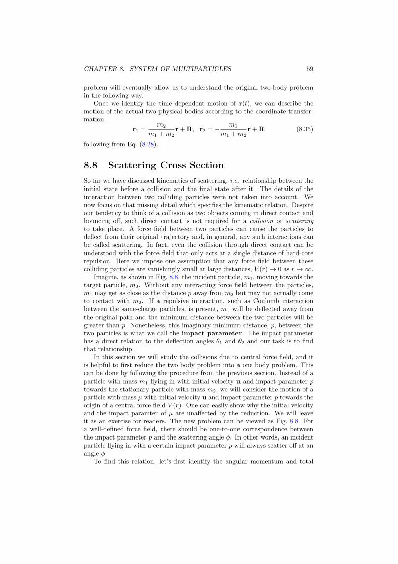
CHAPTER 8. SYSTEM OF MULTIPARTICLES 59
problem will eventually allow us to understand the original two-body problemin the following way.
Once we identify the time dependent motion of r(t), we can describe themotion of the actual two physical bodies according to the coordinate transfor-mation,
r1 =m2
m1 +m2r + R, r2 = − m1
m1 +m2r + R (8.35)
following from Eq. (8.28).
8.8 Scattering Cross Section
So far we have discussed kinematics of scattering, i.e. relationship between theinitial state before a collision and the final state after it. The details of theinteraction between two colliding particles were not taken into account. Wenow focus on that missing detail which specifies the kinematic relation. Despiteour tendency to think of a collision as two objects coming in direct contact andbouncing off, such direct contact is not required for a collision or scatteringto take place. A force field between two particles can cause the particles todeflect from their original trajectory and, in general, any such interactions canbe called scattering. In fact, even the collision through direct contact can beunderstood with the force field that only acts at a single distance of hard-corerepulsion. Here we impose one assumption that any force field between thesecolliding particles are vanishingly small at large distances, V (r)→ 0 as r →∞.
Imagine, as shown in Fig. 8.8, the incident particle, m1, moving towards thetarget particle, m2. Without any interacting force field between the particles,m1 may get as close as the distance p away from m2 but may not actually cometo contact with m2. If a repulsive interaction, such as Coulomb interactionbetween the same-charge particles, is present, m1 will be deflected away fromthe original path and the minimum distance between the two particles will begreater than p. Nonetheless, this imaginary minimum distance, p, between thetwo particles is what we call the impact parameter. The impact parameterhas a direct relation to the deflection angles θ1 and θ2 and our task is to findthat relationship.
In this section we will study the collisions due to central force field, and itis helpful to first reduce the two body problem into a one body problem. Thiscan be done by following the procedure from the previous section. Instead of aparticle with mass m1 flying in with initial velocity u and impact parameter ptowards the stationary particle with mass m2, we will consider the motion of aparticle with mass µ with initial velocity u and impact parameter p towards theorigin of a central force field V (r). One can easily show why the initial velocityand the impact paramter of µ are unaffected by the reduction. We will leaveit as an exercise for readers. The new problem can be viewed as Fig. 8.8. Fora well-defined force field, there should be one-to-one correspondence betweenthe impact parameter p and the scattering angle φ. In other words, an incidentparticle flying in with a certain impact parameter p will always scatter off at anangle φ.
To find this relation, let’s first identify the angular momentum and total
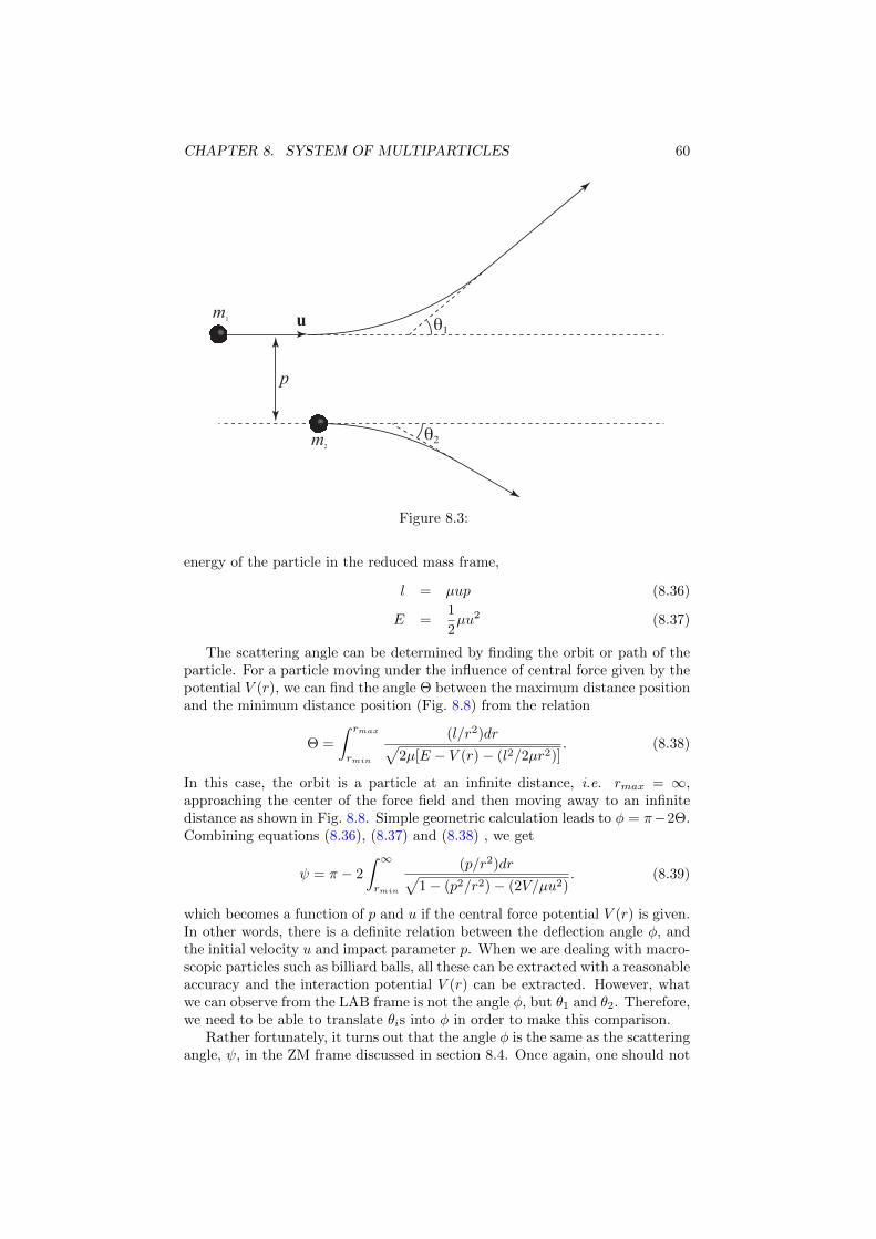
CHAPTER 8. SYSTEM OF MULTIPARTICLES 60
m1
m2
u
p
θ1
θ2
Figure 8.3:
energy of the particle in the reduced mass frame,
l = µup (8.36)
E =1
2µu2 (8.37)
The scattering angle can be determined by finding the orbit or path of theparticle. For a particle moving under the influence of central force given by thepotential V (r), we can find the angle Θ between the maximum distance positionand the minimum distance position (Fig. 8.8) from the relation
Θ =
∫ rmax
rmin
(l/r2)dr√2µ[E − V (r)− (l2/2µr2)]
. (8.38)
In this case, the orbit is a particle at an infinite distance, i.e. rmax = ∞,approaching the center of the force field and then moving away to an infinitedistance as shown in Fig. 8.8. Simple geometric calculation leads to φ = π−2Θ.Combining equations (8.36), (8.37) and (8.38) , we get
ψ = π − 2
∫ ∞rmin
(p/r2)dr√1− (p2/r2)− (2V/µu2)
. (8.39)
which becomes a function of p and u if the central force potential V (r) is given.In other words, there is a definite relation between the deflection angle φ, andthe initial velocity u and impact parameter p. When we are dealing with macro-scopic particles such as billiard balls, all these can be extracted with a reasonableaccuracy and the interaction potential V (r) can be extracted. However, whatwe can observe from the LAB frame is not the angle φ, but θ1 and θ2. Therefore,we need to be able to translate θis into φ in order to make this comparison.
Rather fortunately, it turns out that the angle φ is the same as the scatteringangle, ψ, in the ZM frame discussed in section 8.4. Once again, one should not
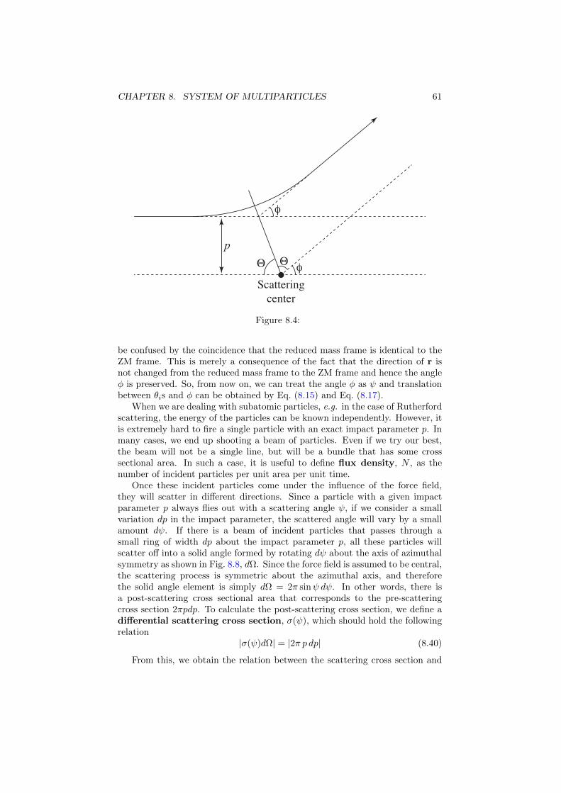
CHAPTER 8. SYSTEM OF MULTIPARTICLES 61
p
φ
φΘ
Scattering
center
Θ
Figure 8.4:
be confused by the coincidence that the reduced mass frame is identical to theZM frame. This is merely a consequence of the fact that the direction of r isnot changed from the reduced mass frame to the ZM frame and hence the angleφ is preserved. So, from now on, we can treat the angle φ as ψ and translationbetween θis and φ can be obtained by Eq. (8.15) and Eq. (8.17).
When we are dealing with subatomic particles, e.g. in the case of Rutherfordscattering, the energy of the particles can be known independently. However, itis extremely hard to fire a single particle with an exact impact parameter p. Inmany cases, we end up shooting a beam of particles. Even if we try our best,the beam will not be a single line, but will be a bundle that has some crosssectional area. In such a case, it is useful to define flux density, N , as thenumber of incident particles per unit area per unit time.
Once these incident particles come under the influence of the force field,they will scatter in different directions. Since a particle with a given impactparameter p always flies out with a scattering angle ψ, if we consider a smallvariation dp in the impact parameter, the scattered angle will vary by a smallamount dψ. If there is a beam of incident particles that passes through asmall ring of width dp about the impact parameter p, all these particles willscatter off into a solid angle formed by rotating dψ about the axis of azimuthalsymmetry as shown in Fig. 8.8, dΩ. Since the force field is assumed to be central,the scattering process is symmetric about the azimuthal axis, and thereforethe solid angle element is simply dΩ = 2π sinψ dψ. In other words, there isa post-scattering cross sectional area that corresponds to the pre-scatteringcross section 2πpdp. To calculate the post-scattering cross section, we define adifferential scattering cross section, σ(ψ), which should hold the followingrelation
|σ(ψ)dΩ| = |2π p dp| (8.40)
From this, we obtain the relation between the scattering cross section and
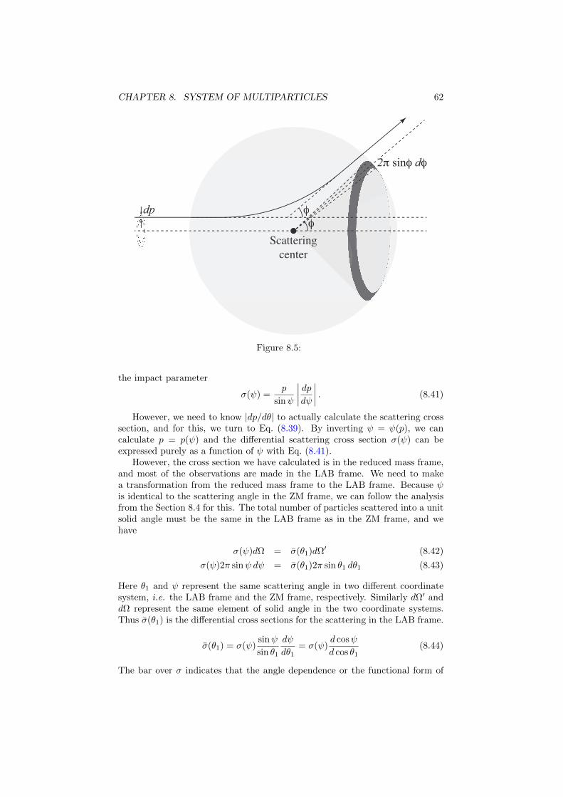
CHAPTER 8. SYSTEM OF MULTIPARTICLES 62
φ
Scattering
center
φ
Scattering
center
dp
φ
2π sinφ dφ
Figure 8.5:
the impact parameter
σ(ψ) =p
sinψ
∣∣∣∣ dpdψ∣∣∣∣ . (8.41)
However, we need to know |dp/dθ| to actually calculate the scattering crosssection, and for this, we turn to Eq. (8.39). By inverting ψ = ψ(p), we cancalculate p = p(ψ) and the differential scattering cross section σ(ψ) can beexpressed purely as a function of ψ with Eq. (8.41).
However, the cross section we have calculated is in the reduced mass frame,and most of the observations are made in the LAB frame. We need to makea transformation from the reduced mass frame to the LAB frame. Because ψis identical to the scattering angle in the ZM frame, we can follow the analysisfrom the Section 8.4 for this. The total number of particles scattered into a unitsolid angle must be the same in the LAB frame as in the ZM frame, and wehave
σ(ψ)dΩ = σ(θ1)dΩ′ (8.42)
σ(ψ)2π sinψ dψ = σ(θ1)2π sin θ1 dθ1 (8.43)
Here θ1 and ψ represent the same scattering angle in two different coordinatesystem, i.e. the LAB frame and the ZM frame, respectively. Similarly dΩ′ anddΩ represent the same element of solid angle in the two coordinate systems.Thus σ(θ1) is the differential cross sections for the scattering in the LAB frame.
σ(θ1) = σ(ψ)sinψ
sin θ1
dψ
dθ1= σ(ψ)
d cosψ
d cos θ1(8.44)
The bar over σ indicates that the angle dependence or the functional form of

CHAPTER 8. SYSTEM OF MULTIPARTICLES 63
σ(θ1) is not identical to that of σ(ψ). Eventually, one should be able to derive
d cosψ
d cos θ1=
d
d cos θ1
m1
m2
− sin2 θ1 ± cos θ1
√(m2
m1
)2
− sin2 θ1
(8.45)
= ± [γ cos θ1 ±√
1− γ2 sin θ1]2√1− γ2 sin θ1
(8.46)
where γ ≡ m1/m2. Also by inverting the Eq. (8.15), we can derive ψ =sin−1(γ sin θ1) + θ1. Substituting ψ for this relation in σ(ψ) for Eq. (8.44),we get σ(θ1) purely as a function of θ1.
8.9 Rutherford Scattering Formula
We take a look at a very special case of the particle scattering we have discussedso far. Hans Geiger and Enest Marsden in 1909 struck a gold foil with a beamof α-particles, i.e. He2+, under the direction of Ernest Rutherford. Although itwas not fully understood at the moment, the interaction between the α-particlesand the gold foil is mostly due to Coulomb interaction between the α-particlesand the positively charged nuclei of gold obeying the relation V = k
r ≡q1q2
4πε0rwith q1 and q2 the amounts of charge that the two interacting particles carry.
Substituting V = k/r in Eq. 9.63, we get
ψ = π − 2
∫ ∞rmin
(b/r)dr√r2 − (k/E)r − b2
. (8.47)
Carrying out the integration in the right hand side with κ ≡ k2E results in the
relation
cos Θ =κ/b√
1 + (κ/b)2(8.48)
Rewriting Eq. 9.68 as tan Θ = b/κ and using the relation ψ = π − 2Θ, b isexpressed in terms of ψ: b = k cot(ψ/2). The scattering cross section is
σ(ψ) =κ2
2
cot(ψ/2)
sinψ sin2(ψ/2)=κ2
2
1
sin4(ψ/2)=
k2
(4E)2
1
sin4(ψ/2)(8.49)
8.10 Angular Momentum
We now turn our focus to the angular momentum of multi-particle systems.Unlike the linear momentum, the angular momentum has to be defined withrespect to a point. The total angular momentum about the origin of a givencoordinate system O, LO, is the sum of angular momentum of all the individualparticles, li = ri × pi = ri × (miri), in the system.
LO =∑i
Li =∑i
ri × (miri) (8.50)
Earlier, we have shown that the rate of change in total angular momentum ofthe system about a point O is equal to the net resultant external torques aboutthat point, that is,
dLOdt
= KO (8.51)

CHAPTER 8. SYSTEM OF MULTIPARTICLES 64
We can also define angular momentum of the system with respect to a generalpoint A rather than O. The position vector of the i-th particle about A is givenby ri − a and assuming that the point A is fixed within the coordinate frame,LA becomes
LA =∑i
(ri − a)× (miri) =∑i
ri × (miri) − a×∑i
miri
= LO − a×P (8.52)
with the total linear momentum of the system, P, is identified as Eq. (8.5). Theangular momentum, LA, of a particle, P , with respect to a point, A, is alwaysperpendicular to the plane containing A, P and the velocity of the particler. The component of the angular momentum about an arbitrary axis n byprojecting the angular momentum vector LA onto n:
LA · n = ρp · φ (8.53)
where ρ is the perpendicular distance of the particle from the axis and p · φ isthe azimuthal component of p around the axis.
If we let the point A move around inside our coordinate frame, then
LA =∑i
(ri − a)×mi(ri − a)
=∑i
ri × (miri) − a×∑i
miri −∑i
miri × a +∑i
mia× a
= LO − a×P−MR× a +Ma× a (8.54)
From this, we can invoke an interesting feature about angular momentum. Ifwe choose our point A to be the center of mass of the system, G, the last twoterms cancel each other, and we are left with the relation
LO = LG + R×P (8.55)
Total angular momentum about an origin is the sum of the angular momentumof the center of mass about that origin and the angular momentum of the systemabout the position of the center of mass. From this relation, we can also deducethat
dLGdt
= KG (8.56)
In any motion of a system S, the rate of increase of the angular momentumabout the CM is equal to the total moment about the CM of the external forcesacting on S, regardless of the motion of the center of mass.
8.11 Energy of the System
In chapter 2, we’ve learned that the total energy, E = T + V , of a particle ina conservative force field is a constant, where T is the kinetic energy and U isthe potential energy. Is this true for a system of many particles? If the systemgets rearranged from a certain configuration 1 to a different configuration 2 by
CHAPTER 8. SYSTEM OF MULTIPARTICLES 65
the total force acting on the system, that means some work, W12, is done onthe system,
W12 =∑i
∫ 2
1
Fneti · dri =
∑i
∫ 2
1
Fi · dri +∑i
∑j 6=i
∫ 2
1
Gij · dri (8.57)
=∑i
∫ 2
1
Fi · dri +∑i<j
(∫ 2
1
Gij · dri +
∫ 2
1
Gji · dri)
(8.58)
= −∑i
∫ 2
1
∇iVi · dri −∑i<j
(∫ 2
1
∇iVij · dri +
∫ 2
1
∇j Vji · dri)(8.59)
= −∑i
∫ 2
1
dVi −∑i<j
∫ 2
1
dVij =
−(∑i
Vi +∑i<j
Vij)
2
1
(8.60)
Going from Eq. (8.58) to Eq. (8.57), we used the assumption that the forcefield is conservative, that is, the forces Fi and Gij are derivable from potentialfunctions Vi and Vij , respectively. We can define the total potential energyV = −(
∑i Vi +
∑i<j Uij), and we get
W12 = V1 − V2. (8.61)
In terms of kinetic energy, the work done on the system is
W12 =∑i
∫ 2
1
d
(1
2miv
2i
)= T2 − T1. (8.62)
where T =∑i
12miv
2i . Combining Eq. (8.57) and Eq. (8.62), we get W12 =
v1 − V2 = T2 − T1 and thus E = V1 + T1 = V2 + T2. This means: The totalenergy for a conservative system is constant.
The kinetic energy, when written out, is
T =∑i
1
2miv
2i =
∑i
1
2mi|ri|2 =
∑i
1
2mi(R + r′i) · (R + r′i) (8.63)
=∑i
1
2mi(R · R + r′i · r′i + 2R · r′i) (8.64)
=∑i
1
2miV
2 +∑i
1
2miv
′2i + R · d
dt(∑i
mir′i) (8.65)
=1
2MV 2 +
∑i
1
2miv
′2i (8.66)
which can be stated: The total kinetic energy of the system is equal to the sum ofthe kinetic energy of a particle of mass M moving with the velocity of the centerof mass and the kinetic energy of motion of the individual particles relative tothe center of mass.
Finally we return to the problem of high jumping. A human body, of course,is a system of particles. When we high jump, we kick off the ground and gainsome momentum in vertical direction. The jumper will have kinetic energyassociated with that momentum and it will allow the jumper’s center of mass
CHAPTER 8. SYSTEM OF MULTIPARTICLES 66
to reach a certain height. Ignoring small amount of kinetic energy associatedwith moving body parts here and there, the final height of the jumper’s centerof mass is more or less given by the amount of momentum he or she picks upat the time of kicking off the ground. So the most effective way to high jumpwould be to find a way to put your center of mass outside your body and haveyour body parts actually role around the center of mass. That is exactly whatthese high jumpers are doing.
The most traditional method known as the scissors technique looks quitenatural and easy, but the center of mass actually has to clear the height of thebar and thus is not very effective. Straddle technique or Fosbury flop are moreadvanced techniques and lets you clear higher bars because the center of massactually goes under the bar, and therefore widely used these days.

Chapter 9
Rigid Body Kinematics
In this chapter, we will turn our attention away from particles and focus onrigid bodies. The rigid body is defined to be a system in which the distancebetween any pair of composing particles is fixed, that is, for any two points,Pi and Pj , on the rigid body represented by position vectors ri and rj , thefollowing relationship holds for all time t
|ri − rj | = cij (9.1)
where the cij are constant. One can show that the above definition of rigidityis equivalent to
ri · rj + ri · rj = 0 (9.2)
For a rigid body, the main feature in understanding its dynamics heavilyrelies on distinguishing translational and rotational motions.
9.1 Rotation and Linear Velocity
In two dimensional space, rotation axis is always perpendicular to the planeof motion, and angular velocity can be treated as a scalar. However, in threedimensional space, the rotation axis can take arbitrary direction, say n and it isuseful to identify (right-handed) angular velocity as a vector along the rotationaxis,
ω = ωn (9.3)
We will leave proving that the angular velocity can be represented by a vectoras an exercise for the readers. The fact that the angular velocity is a vectorhas a rather interesting implications, which is that the angular velocity can bedecomposed into two or more vector components:
ω = ω1 + ω2. (9.4)
At first glance, this might seem like a rather unintuitive and unnecessary prop-erty of the angular velocity, but it will become extremely useful later.
With the angular velocity represented as a vector, the linear velocity of anypoint, P , within a rotating rigid body can be obtained by
v = ω × (r− b) (9.5)
67
CHAPTER 9. RIGID BODY KINEMATICS 68
where r is the position vector of P and b is the position vector of any fixed point,B, on the rotation axis. In other words, the point P has a relative velocity withrespect to the point B given by ω × (r− b). Here, one should note that therotation axis including the point B does not necessarily have to go through therigid body.
If the point B has a translational velocity vB with respect to some fixedcoordinate system, because of the definition of rigidity, every point on the bodymust have the same translational velocity vB . Then the net linear velocity ofthe point P should be the vector sum of vB and ω × (r− b):
v = vB + ω × (r− b) (9.6)
The above relation results in a rather interesting property of the rigid body. Letus consider two different points A and P , then the velocity of these two pointscan be given by
vA = vB + ω × (a− b) (9.7)
v = vB + ω × (r− b) (9.8)
where a is the position vector of A. Subtracting Eq. 9.7 from Eq. 9.8, we get
v = vA + ω × (r− a) (9.9)
What this states is that the velocity of the point P on the rigid body can bedecomposed to the translational velocity of any point A, vA within the rigidbody and the rotational velocity of P with respect to A, ω × (r− a). Oneshould pay attention to the fact that the point A can be any point within therigid body not necessarily along the rotating axis originally considered. In thisregard, it is fair to say that there is no single fixed rotating axis in a rigid body.Any point on the rigid body is rotating about another point on rigid body withthe identical angular velocity ω.
9.2 Moment of Inertia Tensor
As we have seen in the previous section, velocity of particles within a rigidbody can be dissected into the linear velocity of a reference point and rotationalvelocity with respect to that reference point. This feature allows us to interpreta motion of a rigid body in a dramatically simpler manner.
The ultimate goal in mechanics is to be able to find the positions and ve-locities of particles as functions of time. The fact that the velocity of a rigidbody with respect to a reference point is simply rotational velocity given byω × (r− a) in Eq. (9.9) indicates that when a motion of any single particlewithin the rigid body is given, all we are left is to find the rotational motionabout that point.
Thus, the starting point in rigid body dynamics naturally becomes writingout the angular momentum:
LO =∑α
rα × pα (9.10)
where rα is the position of α-th particle relative to the fixed point. If the an-gular momentum is defined with respect to the reference point of the rotational

CHAPTER 9. RIGID BODY KINEMATICS 69
motion, the linear momentum of the α-th particle, pα, can be expressed aspα = mαω × rα and therefore
LO =∑α
mαrα × (ω × rα). (9.11)
Using the vector identity A× (B×A) = A2B−A(A ·B) (or [A× (B×A)]i =BiA
2 −Ai(A ·B)), the i-th component of LO is expressed as
Li =∑α
mα
ωi∑k
r2α,k − rα,i
∑j
rα,jωj
=
∑α
mα
∑j
(ωjδij
∑k
r2α,k − ωjrα,irα,j
)
=∑j
ωj∑α
mα
(δij∑k
r2α,k − rα,ixα,j
)(9.12)
where the relation ωi =∑j δijωj is used going from the second line to the third
line. The δij is defined as
δij =
0 if i 6= j1 if i = j
(9.13)
The Greek lettered indices α, β, γ, etc. represent each particle and the Italic in-dices i, j and k represent the three components in Cartesian coordinate system,that is, rα,i is the i-th Cartesian component of the α-th particle, or rα,1 = xα,rα,2 = yα and rα,3 = zα.
If we define Iij as
Iij ≡∑α
mα
(δij∑k
r2α,k − rα,ixα,j
), (9.14)
we can rewrite the Eq. (9.12):
Li =∑j
Iijωj (9.15)
The above equation can be rewritten in matrix notation, L = I · ω. Here, Land ω are three dimensional vectors representing the angular momentum andangular velocity, respectively, and I is a three-by-three matrix. The elementsof the matrix I denoted as Iij are referred to as the moment of inertia tensors.They represent the moment of inertia associated with the angular velocity in thej-th component that contributes to angular momentum in the i-th component.
From the Eq. (9.12), we can see that the angular momentum along the ri-axis is a result of rotation along all three x, y and z-axes, ωx, ωy and ωz. Inother words, a general rotation given by an angular velocity in three dimensionalspace is not necessarily colinear with the angular momentum. In describing arotational motion, the moment of inertia must be able to identify such non-colinearity, which is done by utilizing tensor representation.
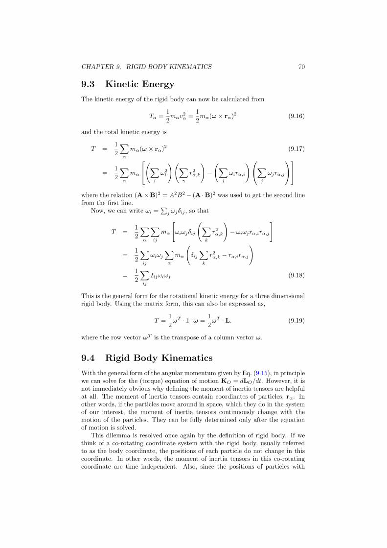
CHAPTER 9. RIGID BODY KINEMATICS 70
9.3 Kinetic Energy
The kinetic energy of the rigid body can now be calculated from
Tα =1
2mαv
2α =
1
2mα(ω × rα)2 (9.16)
and the total kinetic energy is
T =1
2
∑α
mα(ω × rα)2 (9.17)
=1
2
∑α
mα
(∑i
ω2i
)(∑γ
r2α,k
)−
(∑i
ωirα,i
)∑j
ωjrα,j
where the relation (A×B)2 = A2B2− (A ·B)2 was used to get the second linefrom the first line.
Now, we can write ωi =∑j ωjδij , so that
T =1
2
∑α
∑ij
mα
[ωiωjδij
(∑k
r2α,k
)− ωiωjrα,irα,j
]
=1
2
∑ij
ωiωj∑α
mα
(δij∑k
r2α,k − rα,irα,j
)
=1
2
∑ij
Iijωiωj (9.18)
This is the general form for the rotational kinetic energy for a three dimensionalrigid body. Using the matrix form, this can also be expressed as,
T =1
2ωT · I · ω =
1
2ωT · L. (9.19)
where the row vector ωT is the transpose of a column vector ω.
9.4 Rigid Body Kinematics
With the general form of the angular momentum given by Eq. (9.15), in principlewe can solve for the (torque) equation of motion KO = dLO/dt. However, it isnot immediately obvious why defining the moment of inertia tensors are helpfulat all. The moment of inertia tensors contain coordinates of particles, rα. Inother words, if the particles move around in space, which they do in the systemof our interest, the moment of inertia tensors continuously change with themotion of the particles. They can be fully determined only after the equationof motion is solved.
This dilemma is resolved once again by the definition of rigid body. If wethink of a co-rotating coordinate system with the rigid body, usually referredto as the body coordinate, the positions of each particle do not change in thiscoordinate. In other words, the moment of inertia tensors in this co-rotatingcoordinate are time independent. Also, since the positions of particles with
CHAPTER 9. RIGID BODY KINEMATICS 71
i
j
k
e1
e3
e2O
Figure 9.1: Angular velocity and angular momentum representing a generalrotation of a dumbell.
respect to the body coordinate are fixed, we can track the motion of the rigidbody by following how the body coordinate moves in time. In other words, rigidbody kinematics is a matter of identifying the orientation of the body coordinatewith respect to the fixed coordinate.
From here on, we will denote the unit vectors for three Cartesian componentsof the fixed coordinate and the body coordinate with i, j, k and e1, e2, e3,respectively.
9.5 Principal Axes of Inertia
Things are considerably simpler to describe rotation in two dimensions. Bothangular velocity and angular momentum are in the same direction, perpendic-ular to the two dimensional surface and the moment of inertia is always scalar.In three dimensional space, this is generally not the case. Only when certainsymmetry conditions are met, rotation of a rigid body can be described in amanner similar to that of two dimensions.
Imagine a dumbbell connected by masses m1 and m2 at the ends of itsshaft as shown in Fig. 9.5. In general, the angular velocity ω and the angularmomentum L are not collinear, i.e. they are not along the same direction. Inother words, ω and L are not connected by a scalar number. There are however,two distinct cases in which ω and L are collinear. One case is when the rotation

CHAPTER 9. RIGID BODY KINEMATICS 72
x
y
z
ωL
Figure 9.2: Angular velocity and angular momentum representing a generalrotation of a dumbell.
axis is along the shaft of the dumbbell, and the other is when the rotation axisis perpendicular to the dumbbell. These particular set of axes are called theprincipal axes of inertia. In general physics, rotation was always thought to betaking place along these axes. Thus, the relation between the angular velocityand angular momentum could be expressed as
L = Iω (9.20)
with I as a scalar number representing the moment of inertia for the rotationalong the principal axis.
The relation Eq. (9.20) can be used to find the principal moment of axesfor a rigid body within the given coordinate system. When a body is rotatingabout a principal axis, we set the angular momentum vector L = Iω to be equalto L = I · ω. Lx = Iωx = Ixxωx + Ixyωy + Ixzωz
Ly = Iωy = Iyxωx + Iyyωy + IyzωzLz = Iωz = Izxωx + Izyωy + Izzωz
(9.21)
We can rewrite the equations as follows (Ixx − I)ωx + Ixyωy + Ixzωz = 0Iyxωx + (Iyy − I)ωy + Iyzωz = 0Izxωx + Izyωy + (Izz − I)ωz = 0
(9.22)
For ωαs to have non-trivial solutions, the determinant of the coefficients has tobe zero. ∣∣∣∣∣∣
Ixx − I Ixy IxzIyx Iyy − I IyzIzx Izy Izz − I
∣∣∣∣∣∣ = 0 (9.23)
The equation is third order equation with respect to I and yields three valuesof I: A, B and C. For each value of Iχ = A,B,C (χ = A,B,C), we can find
CHAPTER 9. RIGID BODY KINEMATICS 73
the ratio between ωχx , ωχy and ωχz by solving the equation(Ixx − Iχ)ωχx + Ixyω
χy + Ixzω
χz = 0
Iyxωχx + (Iyy − Iχ)ωχy + Iyzω
χz = 0
Izxωχx + Izyω
χy + (Izz − I)ωχz = 0
(9.24)
This ratio defines the direction of ωχ along which the moment of inertia has thescalar value Iχ. In other words, the direction defined by ωχs are the principalaxes of inertia. In linear algebraic terms, this is the eigenvalue and eigenvectorproblem, where the principal axes represented by ωχ are eigenvalues associatedto the principal moment of inertia, the eigenvectors.
Using the fact that the moment of inertia tensor is symmetric one can showthat the principal axes are orthogonal to one another, that is, ωχ · ωφ = 0 forχ 6= φ. Strictly speaking, if two or three of Iχs have the same value, ωχs neednot be orthogonal to each other. Nonetheless, one can always find orthogonalset of ωχs that satisfies Eq. (9.24). We will leave it to the readers to prove thispoint. (The proof falls into category of linear algebraic problem than a classicalmechanics problem.)
Because we now have three orthogonal axes as our princial axes, we can usethem as our bases of a coordinate system. In other words, we can representany vector as a linear combination of three vectors along e1, e2 and e3 wheree1 ‖ ωA, e2 ‖ ωB and e3 ‖ ωC .
An important feature of the principal axes is that if we choose them as ourbasis for the coordinate system, the moment of inertia tensor becomes diagonal,that is
I =
I11 I12 I13
I21 I22 I23
I31 I32 I33
=
A 0 00 B 00 0 C
(9.25)
where the subscripts of Iijs come from the indices of ei. Therefore the rotationpresented within this coordinate system can be expressed through the followingrelations
T =1
2
∑i
Iiiω2i (9.26)
Li = Iiiωi (9.27)
which are considerably simpler than Eq. (9.18) and (9.12). Due to this simplicity,the principal axes of inertia is an excellent choice as the body coordinate.
9.6 Moments of Inertia for Different Body Co-ordinate Systems
There are cases when the moment of inertia tensor is given in a particular setof body coordinate system, e.g. with the origin of the coordinate system at thecenter of mass of a rigid body. However, if the body is rotating with the pivotpoint of rotation not at the center of mass, it is helpful to understand how inertiatensor transforms from the center-of-mass coordinate system to a different bodycoordinate system. Let’s denote three orthogonal axes of the center-of-masscoordinate system with ris. If we pick another body coordinate system with a

CHAPTER 9. RIGID BODY KINEMATICS 74
set of axes Ris that has same orientation as the center-of-mass coordinate andis separated by distance a, the translational displacement between the two bodycoordinate systems is then a, i.e. R = a + r.
If we substitute each component Ri with ai + xi, for inertia tensor in thesecond body coordinate system, Jij , we get
Jij =∑α
mα
(δij∑k
X2α,k −Xα,iXα,j
)(9.28)
= Iij +M(a2δij − aiaj) (9.29)
where Iij is the original moment of inertia tensor defined at the center-of-massbody coordinate system and M is the total mass of the rigid body. We willleave the detailed calculation as an exercise for the readers.
The second term in the above equation, M(a2δij − aiaj) is simply momentof inertia of a point particle sitting at a poition a with respect to the origin.In other words, the moment of inertia tensor in a different coordinate system isthe sum of original moment of inertia tensor and the moment of inertia due toa particle with mass M . It can be also shown from this that the orientation ofthe body coordinates are not affected if the displacement vector a along one ofthe three principal axes.
9.7 Euler’s Equations
Now that we have established the methods for representing rotational dynamics,we will set up equations of motion:
F =dP
dt(9.30)
KG =dLGdt
(9.31)
where the first equation is for the translational motion of the center of mass, andthe second equation for the rotational motion about the center of mass. If therigid body has a fixed pivot O different from the center of mass, the equationof motion can be reduced to a single torque equation
KO =dLOdt
(9.32)
We will rewrite this equation within the body coordinate system. With ω =ω1e1 + ω2e2 + ω3e3, the angular momentum is expressed as
L = Aω1e1 +Bω2e2 + Cω3e3 (9.33)
and the equation of motion is then
K =d
dt
(IAω1e1 + IBω2e2 + ICω3e3
)= Aω1e1 +Bω2e2 + Cω3e3
+Aω1e1 +Bω2e2 + Cω3e3 (9.34)
CHAPTER 9. RIGID BODY KINEMATICS 75
Note that the coordinate axes are locked to the rigid body, and thus the momentof inertia tensor is unaltered within this coordinate system. Instead, the coor-dinate axes eis are time dependent. Because the coordinate axes are changingwith time due to the rotation of the rigid body, the following relation holds,from Eq. (9.5),
ei = ω × ei (9.35)
By plugging ω = ω1e1 + ω2e2 + ω3e3 into the above equation, Eq. (9.34) isreduced to
K1 = Aω1 − (B − C)ω2ω3
K2 = Bω2 − (C −A)ω3ω1 (9.36)
K3 = Cω3 − (A−B)ω1ω2
which is known as the Euler’s equations. The equations look quite attractivedue to their symmetry, but all the vectors including the torque are decomposedin the body coordinate. Therefore, unless the torque can be easily identified inthe body coordinate, the equations are actually not quite useful.
9.8 Free Body Rotation of a Rigid Body withAxial Symmetry
A general motion of a rigid body is extremely complicated to solve, but thereare a few cases where the solution comes out in a rather straightforward fashion.One of such problems is the rotation of an axisymmetric body with respect tothe center-of-mass in the absence of external torque. Here an axisymmetric body(or a body with axial symmetry) means a body with a cylindrical symmetry, sothat A = B.
The angular velocity, ω, expressed in terms of the axial unit vector, e3, is
ω = ω3e3 + e3 × e3 (9.37)
The first term represents the angular velocity component along the symmetricaxis, e3 and the second term is the angular velocity component perpendicularto the symmetric axis. Thus the angular momentum can be written as
L = Ae3 × e3 + Cω3e3 = constant (9.38)
where the first term comes from the axial symmetry. Because the system hascylindrical symmetry, we can choose any axis that is perpendicular to e3 as aprincipal axis, and the moment of inertia along such axis is equal to A. Sincethere is no external torque acting on the system, the angular momentum L mustbe conserved.
Because the angular momentum is conserved, the following relation is alsotrue:
e3 ·dL
dt= Cω3 = 0 (9.39)
which implies that the axial component of the angular velocity, ω3 does notchange with time, even though the symmetric axis itself is not constant.

CHAPTER 9. RIGID BODY KINEMATICS 76
Taking the dot product between e3 and L results in
e3 · L = Cω3 = constant (9.40)
Thus the angle between the angular momentum and the symmetric axis is alsoconstant in time.
This time, we will take the cross product between e3 and L and get
e3 × L = Ae3 × (e3 × e3) + Cω3e3 × e3
= −Ae3 (9.41)
By rearranging the above equation, the following can be identified
e3 =L
A× e3 = Ω× e3 (9.42)
where Ω ≡ L/A. This equation states that the symmetry axis e3 precessesaround the angular momentum axis L with constant angular speed L/A.
We will rewrite the angular velocity as
ω = e3 × e3 + ω3e3
= e3 ×(
L
A× e3
)+
e3 · LC
e3
=L
A+ e3 · L
(A− CAC
)e3 (9.43)
This can be decomposed as angular velocity of the symmetric axis e3 aboutthe fixed angular momentum axis L and the angular velocity of the rigid bodyabout the symmetric axis e3. In other words, the rigid body rotates about e3
with an angular speed e3 · L(A−CAC
)and the rotating body precesses about the
fixed axis with an angular speed L/A.The same result can be derived by solving the Euler’s equations from the
previous section. One can also show that three vectors L, ω3 and e3 are all onthe same plane, which is a good vector calculus exercise for the readers.
9.9 Precession of a Symmetric Top due to a WeakTorque
Consider a symmetric top whose inertia tensor takes the form
I =
A 0 00 A 00 0 C
(9.44)
relative to the top’s principal axes, e1, e2 and e3. Here e3 is the symmetry axis,and e1 and e2 can be chosen to be any two orthogonal axes perpendicular toe3. See Fig. 9.9.
If the rotation of the body is about the axis of symmetry, i.e. ω = ω3e3, theangular momentum is simply,
L = Cω = Cω3e3 (9.45)
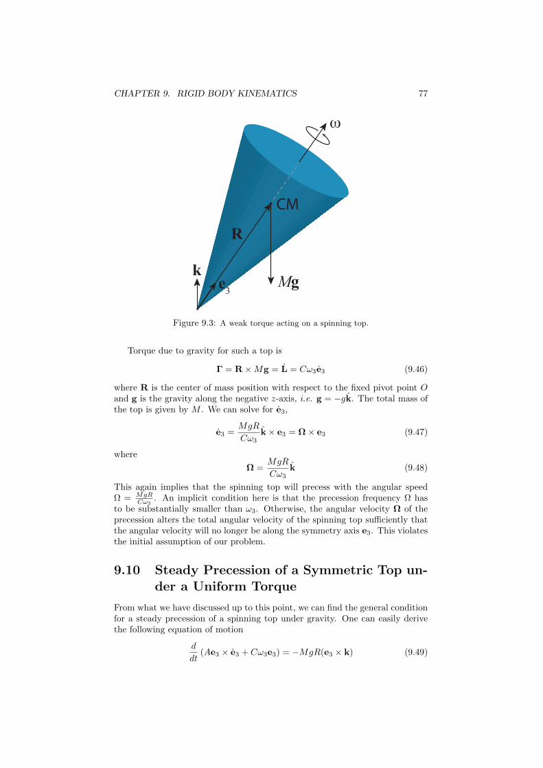
CHAPTER 9. RIGID BODY KINEMATICS 77
CM
Mg
R
ω
e3
k
Figure 9.3: A weak torque acting on a spinning top.
Torque due to gravity for such a top is
Γ = R×Mg = L = Cω3e3 (9.46)
where R is the center of mass position with respect to the fixed pivot point Oand g is the gravity along the negative z-axis, i.e. g = −gk. The total mass ofthe top is given by M . We can solve for e3,
e3 =MgR
Cω3k× e3 = Ω× e3 (9.47)
where
Ω =MgR
Cω3k (9.48)
This again implies that the spinning top will precess with the angular speedΩ = MgR
Cω3. An implicit condition here is that the precession frequency Ω has
to be substantially smaller than ω3. Otherwise, the angular velocity Ω of theprecession alters the total angular velocity of the spinning top sufficiently thatthe angular velocity will no longer be along the symmetry axis e3. This violatesthe initial assumption of our problem.
9.10 Steady Precession of a Symmetric Top un-der a Uniform Torque
From what we have discussed up to this point, we can find the general conditionfor a steady precession of a spinning top under gravity. One can easily derivethe following equation of motion
d
dt(Ae3 × e3 + Cω3e3) = −MgR(e3 × k) (9.49)

CHAPTER 9. RIGID BODY KINEMATICS 78
Steady precession is a precession of a top in which the angle, α, between theaxial vector e3 and the vertical k and the precession frequency are fixed, i.e.e3 · k = cosα = constant and Ω = constant. In such steady precession, the rateof change of e3 is given by
e3 = Ωk× e3 (9.50)
If such motion is possible, one should be able to rewrite the first term in theEq. (9.49) as
d
dt(Ae3 × e3) = A
d
dte3 × (Ωk× e3)
= AΩd
dt(k− cosα e3)
= AΩ2 cosα (e3 × k) (9.51)
and the second term as
d
dt(Cω3e3) = Cω3e3 = −Cω3Ω(e3 × k) (9.52)
Using the relations given by Eq. (9.51) and (9.52), Eq. (9.49) can be simplifiedto
(A cosαΩ2 − Cω3Ω +MgR)(e3 × k) = 0 (9.53)
For the precession frequency Ω to have a real value, the following condition hasto be met
(Cω3)2 ≥ 4AMgR cosα (9.54)
One can easily show that for the case (Cω3)2 4AMgR cosα, two solutions tothe quadratic equation for Ω,
A cosαΩ2 − Cω3Ω +MgR = 0 (9.55)
becomes the two different precession frequencies obtained in the previous twosections:
ΩF ≈ L
Aand ΩS ≈ MgR
Cω3(9.56)
Readers can ponder upon the meaning of this statement.
9.11 Eulerian Angles
So far, we have learned how to describe rotation of rigid body in a few specialcases. Directly solving for the equation of motion or a rigid body is, in mostcases, not at all straightforward. Instead, one can utilize Lagrangian mechanicswhich requires an appropriate choice of generalized coordinates. One widelyused generalized coordinates are the Eulerian angles.
To understand what Eulerian angles are, we have to rethink about the re-lation between the fixed coordinate system and the body coordinate systemwhich is geometrically locked to the rigid body of interest. Since both coordi-nate systems are orthogonal three dimensional coordinate systems, there mustbe a coordinate transformation that transforms the fixed coordinates into thebody coordinates and vice versa. If the two coordinate systems share a commonorigin, the coordinate transformation is a set of rotations.
CHAPTER 9. RIGID BODY KINEMATICS 79
There is always a single rotation about a particular axis that will transformthe fixed coordinates into the body coordinates. However, this is not the sim-plest method as it requires four parameters: three parameters to identify theaxis of rotation and the forth parameter to identify the amount of rotation, i.e.the angle of rotation. Instead, a series of three rotations about known axes cando the job just as well. There are different choices for such series of rotations,but we will follow the method developed by Euler.
Consider the following series of rotations, which takes the x′i system into thexi system.
1. Rotation by φ counterclock-wise about x′3-axis: the transformation leadsto x′′1
x′′2x′′3
=
cosφ sinφ 0−sinφ cosφ 0
0 0 1
x′1x′2x′3
(9.57)
Because the rotation took place about the x′3-axis, it is unaffected by therotation and x′′3 = x′3.
2. Rotation by θ counterclock-wise about x′′1 -axis: x′′′1x′′′2x′′′3
=
1 0 00 cosθ sinθ0 −sinθ cosθ
x′′1x′′2x′′3
(9.58)
This rotation will lead to the x′′′i system with x′′1 = x′′′1 .
3. Finally, rotation by ψ counterclock-wise about x′′′3 (= x3)-axis: x1
x2
x3
=
cosψ sinψ 0−sinψ cosψ 0
0 0 1
x′′′1x′′′2x′′′3
(9.59)
The final coordinate system is the xi system with x3 = x′′′3 . Since these threesubsequent rotations will result in coordinate transformation from xi system toxi, we can write the relation as
x = λx′ where
λ =
cosψ cosφ− cos θ sinφ sinψ cosψ sinφ+ cos θ cosφ sinψ sinψ sin θ− sinψ cosφ− cos θ sinφ cosψ − sinψ sinφ+ cos θ cosφ cosψ cosψ sin θ
sin θ sinφ − sin θ cosφ cos θ
As difficult as it is for one to see it, the beauty of this is that one can
transform between any two Cartesian coordinate systems that share a commonorigin using this method with three parameters φ, θ and ψ and these threeangles are known as the Eulerian angles.
Our goal was to find appropriate coordinate transformation that yields e1e2e3
system from ijk system. In this case k- and e3-axes play the role of x′3 and x3-axes, respectively and θ is the angle between k and e3, i.e. cos θ = e3 · k. Westill need to identify x′′1 -axis, which turns out to be the straight line formed bythe ij-plane and e1e2-plane. This is equivalent to the axis perpendicular to theplane formed by k and e3 vectors.
CHAPTER 9. RIGID BODY KINEMATICS 80
Therefore, one can get to ei system from the ijk system by 1) rotating the ijkcoordinate system about the k-axis until the i-axis matches i′ = k×e3. We willdenote the amount of rotated angle by φ: φ = cos−1i · (k×e3). 2) Rotate thepreviously achieved coordinate system about i′ by θ = cos−1(e3 ·k). 3) Finally,rotate the coordinate system about e3 until the coordinate axes are all alignedto e1e2e3 system, that is i′ becomes e1. The final angle of rotation is denotedby ψ = cos−1(k × e3) · e1. Note that all the angles can be defined by thebasis vectors of the two coordinate systems between which the transformationis occurring.
9.12 Motion of a Symmetric Top with One PointFixed
If e1e2e3 system represents the body coordinates of a rigid body under rotation,then the basis vectors for this coordinate system e1, e2 and e3 must change withtime. However, this is not a problem per se, since any time dependence of thecoordinate axes can be dumped into the Eulerian angles. Therefore, the rigidbody dynamics simply becomes the matter of finding time dependence of φ(t),θ(t) and ψ(t) and they can be the perfect choice as the generalized coordinates.
This is especially useful considering how ineffective Euler’s equations (Eq. (9.36))are. The problem is that the equations themselves are set up in the body coor-dinate system, and unless the solution is known or guessed correctly in advance,there is no good way to identify the external torque of the system.
To overcome this shortcoming, we will introduce Lagrangian mechanics. Letus first identify angular velocity in terms of Eulerian angles. Angular velocityω can be constructed with vectors having z, x′ and e3 as basis, ω = φ+ θ+ ψ.We will denote
φ = angular speed about z
θ = angular speed about x′ = z× e3
ψ = angular speed about e3
(9.60)
We can consider projection of each of these angular velocities along three bodycoordinate axes, e1, e2 and e3.
φ1 = φ sin θ sinψ
φ2 = φ sin θ cosψ
φ3 = φ cos θ
(9.61)
θ1 = θ cosψ
θ2 = θ sinψ
θ3 = 0
(9.62)
ψ1 = 0
ψ2 = 0
ψ3 = ψ
(9.63)

CHAPTER 9. RIGID BODY KINEMATICS 81
From this, we can write the kinetic energy of the system
T =1
2
∑Iiiω
2i (9.64)
=1
2A(ω2
1 + ω22) +
1
2Cω2
3 (9.65)
=1
2A(φ2 sin2 θ + θ2) +
1
2C(φ cos θ + ψ)2 (9.66)
If the center of mass of the rigid body is distance R away from the rotatingcenter in the body coordinate system, the potential energy of the system is givenby
V = MgR cos θ (9.67)
The Lagrangian L = T − V is cyclical in φ and ψ, therefore
pφ =∂L
∂φ= (A sin2 θ + C cos2 θ)φ+ Cψ cos θ = constant (9.68)
pψ =∂L
∂ψ= C(ψ + φ cos θ) = constant (9.69)
Eq. (9.69) yields
ψ =pψ − Cφ cos θ
C(9.70)
and Eq. (9.70) combined with Eq. (9.68) gives us
φ =pφ − pψ cos θ
A sin2 θ(9.71)
We can then rewrite Eq. (9.70) as
ψ =pψC− (pφ − pψ cos θ) cos θ
A sin2 θ(9.72)
Note that the angular speeds φ and ψ are now expressed in terms of a singlevariable θ.
We now write the total energy of the system
E =1
2A(ω2
1 + ω22) +
1
2Cω2
3 +MgR cos θ (9.73)
which must be constant. Since pψ = Cω3 is constant, 12Cω
23 must also be
constant. Therefore we can define a different energy scale E′ ≡ E − 12Cω
23
which is also constant.
E′ =1
2A(ω2
1 + ω22) +MgR cos θ (9.74)
=1
2A(φ2 sin2 θ + θ2) +MgR cos θ (9.75)
=1
2Aθ2 +
(pφ − pψ cos θ)2
2A sin2 θ+MgR cos θ (9.76)
=1
2Aθ2 + V (θ) (9.77)

CHAPTER 9. RIGID BODY KINEMATICS 82
where V (θ) ≡ (pφ−pψ cos θ)2
2A sin2 θ+ MgR cos θ is the effective potential energy in θ-
space. One can easily see that Eq. (9.77) is a one dimensional problem in θ-spacewith rotational kinetic energy 1
2Aθ2 and effective potential energy V (θ). From
this equation, we can calculate t(θ)
t(θ) =
∫dθ√
(2/A)[E′ − V (θ)](9.78)
and the final result can be inverted to obtain θ(t). Because φ and ψ wereexpressed as functions of θ only in Eq. (9.71) and (9.72), θ(t) can be used tofind φ(t) and ψ(t). Without actually going into the full solution, which cannotbe analytically solved anyways, we can deduce qualitative motion by lookinginto V (θ) in Eq. (9.77). The effective potential is given by
V (θ) ≡ (pφ − pψ cos θ)2
2A sin2 θ+MgR cos θ (9.79)
and one can easily see that the potential diverges at θ = 0 and π due to thesin2 θ in the denominator of the first term. If the total energy of the systemhappens to coincide with the minimum of V (θ), the spinning top will precesssteadily with θ = θ0. Here θ0 satisfies the condition V (θ0) = Vmin. One can findthe precession speed by calculating φ for θ = θ0. The result should be identicalto the solutions to the Eq. (9.55). This is a good exercise for readers.
In general, the angle θ will have a bound motion between some angles θ1
and θ2. One can easily show that the angular velocity about the z-axis is non-zero from Eq. (9.71). Therefore, the general motion of a spinning top includesan oscillation of the top’s symmetry axis between θ1 and θ2 superposed to theprecession around the z-axis. Such oscillatory precession is usually referred to asnutation. Eq. (9.71) can be used to see if φ changes sign at any point, meaningwhether the nutation includes a looping motion.