classic models for the study of microscopic friction
TRANSCRIPT

POST-GRADUATE PROGRAM IN PHYSICSUNIVERSIDADE FEDERAL DO RIO GRANDE DO SUL
Classic models for the study of microscopic frictionModelos clássicos para o estudo do atrito microscópico 1
Student: Maria Luján Iglesias
Thesis submitted to the Universidade Federal do Rio Grande doSul as a partial requirement to obtain the degree of Doctor in Sci-ences, under the supervision of Prof. Dr. Sebastian Gonçalves(Institute of Physics - UFRGS - Porto Alegre (RS), Brasil).
October, 2018
1Project financed by the Scholarship Program Latin American Physics Center and National Center for Scientific andTechnological Development CLAF/CNPq.

I can believe things that are trueand things that aren’t true and
I can believe things where nobodyknows if they’re true or not
Neil Gaiman- American Gods
Acknowledgment
I would like to thank my supervisor Prof. Sebastián Gonçalves for his guidance, encour-agement and support in overcoming numerous obstacles I have faced through my research.
To Prof. V.M. Kenkre and N. Tiwari for the collaboration and contribution to this work.
I am also grateful to the CLAF (Centro Latinoamericano de Física) and CNPq (Con-selho Nacional de Desenvolvimento Científico e Tecnológico) for the scholarship.
To my friends and dear family for the continuous encouragement and to my fiance, Rafael,for his patience and unconditional support.
I

II
Resumo
O atrito é um fenômeno extremamente onipresente, a ponto de que a maior parte do tempo
não percebemos como isso afeta nossas vidas, desde pequenos detalhes até aspectos fun-
damentais. Geralmente é considerado um problema relacionado com a perda de energia
e desgaste das peças das máquinas, mas sem sua existência não ouviríamos o violino, as
unhas seriam inúteis, e a vida não poderia ser possível, pois num regime sem desgaste, o
equilíbrio térmico seria inalcançável. As técnicas experimentais atuais capazes de estudar
a força de atrito, abriram um novo campo de pesquisa envolvendo escalas de comprimento
atômico, chamado de nano-tribologia. Apesar disso, a origem microscópica da força de
atrito permanece principalmente não resolvida até hoje. Nesta tese de doutorado, foi es-
tudada a base da origem da força de atrito, primeiro investigando sua dependência com
a velocidade através do conhecido modelo de Prandtl-Tomlinson para temperatura igual
a zero. A essência da troca de energia, que poderia explicar o surgimento do atrito foi
investigada pela dinâmica entre duas partículas. Uma ligada a uma mola e a outra lançada
em sua direção com certa velocidade, sendo a interação entre elas do tipo gaussiano (curto
alcance). Para simular um substrato mais realista, o sistema de partículas-mola foi esten-
dido para uma disposição periódica de partículas, independentes entre elas, e a partícula
que no primeiro modelo era lançada, foi substituída por uma ponta, geralmente usada para
escanear as superfícies no microscópio de força atômica. A principal técnica utilizada foi
dinâmica molecular, ferramenta ideal para abordar o estudo da dinâmica de sistemas clás-
sicos de muitas partículas.

III
Abstract
Friction is an extremely ubiquitous phenomenon, to the point that most of the time we do
not realize how it affects our lives, from tiny details to fundamental aspects. It is usually
regarded as a nuisance related with the loss of energy and wear of machine parts, but
without it, we would not hear the violin, the nails would be useless, and life could not
be possible because in a wearless regime, the thermal equilibrium would be unattainable.
The current experimental techniques able to study friction forces, opened a new field of
research involving atomic length scales, called nano-tribology. Despite this, the micro-
scopic origin of friction force remains mostly unsolved until date. In this PhD thesis, was
studied the basis of the origin of the friction force, first investigating its dependence with
the velocity through the well-known Prandtl-Tomlinson model for zero temperature. The
essence of the energy exchange that could explain the emergence of friction was inves-
tigated by the dynamics between two particles. One attached to a spring and the other
sliding in its direction with a certain speed. The interaction between them represented
by Gaussian potential (short range). To simulate a more realistic substrate, the spring-
particle system was extended to a periodic arrangement of particles, independent between
them, and the particle that was thrown against it was replaced by a tip, generally used to
scan the surfaces on the atomic force microscope. The main used technique was molecu-
lar dynamics, an ideal tool to address the study the dynamics of many particles classical
systems.

IV

Contents
Acknowledgment I
Resumo II
Abstract III
List of Figures VII
Structure of the thesis 1
1 Introduction 3
1.1 Objective . . . . . . . . . . . . . . . . . . . . . . . . . . . . . . . . . . 5
1.2 Friction: A very old problem . . . . . . . . . . . . . . . . . . . . . . . . 5
1.3 The Standard Model of Dry Friction . . . . . . . . . . . . . . . . . . . . 6
1.3.1 The microscopic approach of Bowden & Tabor . . . . . . . . . . 9
1.4 Experimental Techniques . . . . . . . . . . . . . . . . . . . . . . . . . . 10
1.4.1 Surface Force Apparatus (SFA) . . . . . . . . . . . . . . . . . . 12
1.4.2 Scanning Tunneling Microscopes (STM) . . . . . . . . . . . . . 13
1.4.3 Atomic Force and Friction Force Microscopes (AFM/FFM) . . . 14
1.4.4 Quartz Crystal Microbalance (QCM) . . . . . . . . . . . . . . . 15
2 Theoretical Foundations 17
2.1 Prandtl-Tomlinson Model . . . . . . . . . . . . . . . . . . . . . . . . . . 17
2.1.1 Velocity Dependence of Friction . . . . . . . . . . . . . . . . . . 23
2.2 The Frenkel-Kontorova Model . . . . . . . . . . . . . . . . . . . . . . . 25
V

VI CONTENTS
3 Models and Methods 31
3.1 First Model: Energy exchange in a two particles system . . . . . . . . . . 31
3.2 Second Model: Prandtl-Tomlinson model improved with no ad-hoc dissi-
pation . . . . . . . . . . . . . . . . . . . . . . . . . . . . . . . . . . . . 33
3.3 Molecular Dynamics . . . . . . . . . . . . . . . . . . . . . . . . . . . . 35
3.3.1 Verlet Algorithm . . . . . . . . . . . . . . . . . . . . . . . . . . 36
3.3.2 Velocity Verlet Algorithm . . . . . . . . . . . . . . . . . . . . . 37
4 Results and Discussions 39
4.1 Prandtl-Tomlinson model revisited . . . . . . . . . . . . . . . . . . . . . 39
4.1.1 Small Velocities representation . . . . . . . . . . . . . . . . . . . 42
4.1.2 Transitional and Large Velocities representation . . . . . . . . . . 44
4.2 Two particles interaction . . . . . . . . . . . . . . . . . . . . . . . . . . 47
4.2.1 Non Oscillator . . . . . . . . . . . . . . . . . . . . . . . . . . . 47
4.2.2 Oscillator . . . . . . . . . . . . . . . . . . . . . . . . . . . . . . 48
4.2.3 Soft k (slow oscillations) . . . . . . . . . . . . . . . . . . . . . . 52
4.2.4 Energy loss calculation . . . . . . . . . . . . . . . . . . . . . . . 55
4.3 From one to N particles . . . . . . . . . . . . . . . . . . . . . . . . . . . 59
4.3.1 Time step comparison . . . . . . . . . . . . . . . . . . . . . . . 61
4.4 Single interaction and periodic lattice equivalence . . . . . . . . . . . . . 66
5 Conclusions 69

List of Figures
1.1 Wall painting from 1880 B.C. on the tomb of Djehutihotep. The figure
standing at the front of the sled is pouring water onto the sand(from
Ref. [27]). . . . . . . . . . . . . . . . . . . . . . . . . . . . . . . . . . . 6
1.2 Leonardo da Vinci’s studies of friction. Sketches from the Codex Atlanti-
cus and the Codex Arundel showing experiments to determine: (a) the
force of friction between horizontal and inclined planes; (b) the influence
of the apparent contact area upon the force of friction; (c) the force of
friction on a horizontal plane by means of a pulley and (d) the friction
torque on a roller and half bearing (from Ref. [30]) . . . . . . . . . . . . 6
1.3 EARLY STUDIES OF FRICTION, such as those done in the 18th century
by the French physicist Charles-Augustin de Coulomb, helped to define
the classical laws of friction and attempted to explain the force in terms of
surface roughness, a feature that has now been ruled out as a significant
source (from Ref. [30]). . . . . . . . . . . . . . . . . . . . . . . . . . . . 7
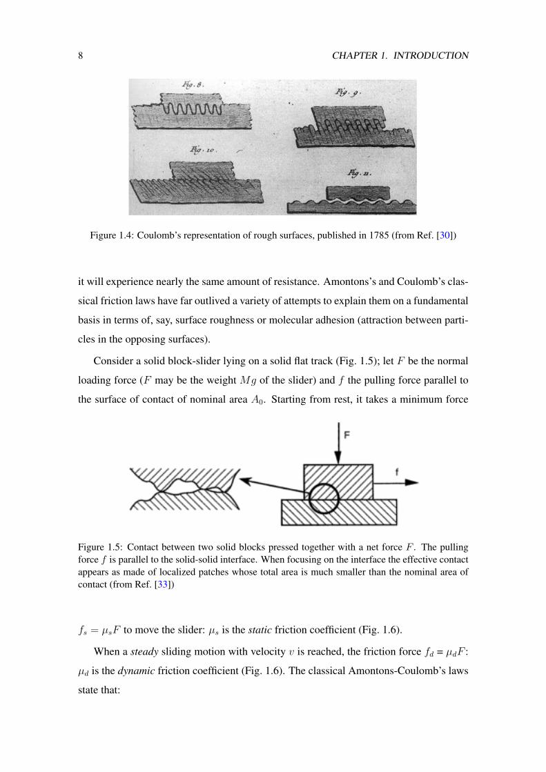
1.4 Coulomb’s representation of rough surfaces, published in 1785 (from
Ref. [30]) . . . . . . . . . . . . . . . . . . . . . . . . . . . . . . . . . . 8
1.5 Contact between two solid blocks pressed together with a net force F .
The pulling force f is parallel to the solid-solid interface. When focusing
on the interface the effective contact appears as made of localized patches
whose total area is much smaller than the nominal area of contact (from
Ref. [33]) . . . . . . . . . . . . . . . . . . . . . . . . . . . . . . . . . . 8
VII

VIII LIST OF FIGURES
1.6 Experimental determination of the friction coefficients for paper- paper.
At t = 0 the slider of mass M is put in contact with the track ; after
a while, the pulling force f is increased from zero at constant velocity;
after a time t = τstick , f = fs = µsMg and the slider moves. Here, after
a transient, the slider achieves steady sliding; the friction force is then
f = fd = µdMg < fs(from Ref. [33]) . . . . . . . . . . . . . . . . . . . 9
1.7 Contact area asperity between two surfaces . . . . . . . . . . . . . . . . 10
1.8 Illustration of the principle of the surface-force apparatus (SFA) for mea-
suring the normal forces, F, and friction of shear forces f , between two
smooth surfaces of area A, separated by a thin liquid film of thickness D.
An optical interference technique allows the shapes of the surfaces and
their separation, D, to be accurately monitored during force and friction
measurements (from Ref. [44]). . . . . . . . . . . . . . . . . . . . . . . . 12
1.9 Diagram of the Scanning Tunneling Microscope . . . . . . . . . . . . . . 13
1.10 Experimental set-up of an AFM/FFM based on the laser beam deflection
method (from Ref. [41]). . . . . . . . . . . . . . . . . . . . . . . . . . . 14
1.11 Front (a) and side (b) views of a QCM. The shaded regions represent
metal electrodes that are evaporated onto the major surfaces of the mi-
crobalance. Molecularly thin solid or liquid films adsorbed onto the sur-
face of these electrodes (which are parallel to the x–z plane) depicted
in (c) may exhibit measurable slippage at the electrode-film interface in
response to the transverse shear oscillatory motion of the microbalance.
The experiment is not unlike pulling a tablecloth out from under a table
setting, whereby the degree of slippage is deter- mined by the friction at
the interface between the dishes (i.e. the adsorbed film material) and the
tablecloth (i.e. the surface of the electrode)(from Ref. [2]). . . . . . . . . 16
2.1 Sketch of the 1D Prandtl-Tomlinson model for atomistic friction. The
cantilever tip of mass m and constant k is moving at constant velocity vc.
The surface is represented as a potential with corrugation U0 and period a 19

LIST OF FIGURES IX
2.2 Time behavior of the tip coordinate (rescaled to the lattice parameter a),
for two values of the reduced corrugation: U0 = 0.5 (below the thresh-
old) and U0 = 3 (above the threshold). While the tip coordinate slides
continuously and the lateral force is smooth for U0 = 0.5, stick-slip oc-
curs for U0 = 3, and the tip velocity has sharp peaks corresponding to the
slip events. The scanning velocity used in the simulations is vc = 0.08
and the damping is assumed to be critical (η = 2). All quantities are in
dimensionless units. . . . . . . . . . . . . . . . . . . . . . . . . . . . . . 20
2.3 Time behavior of the tip velocity for the same conditions as Fig. 2.2. . . . 21
2.4 Time behavior of the lateral force for the same conditions as Fig. 2.2. . . . 21
2.5 Comparison of the tip coordinate (rescaled to the lattice parameter a) for
the undamped and the critically damped case, for U0 = 3. The cantilever
scanning velocity is vc = 0.08. All quantities are in dimensionless units. . 22
2.6 Comparison of the lateral force (rescaled to the lattice parameter a) for
the undamped and the critically damped case, for U0 = 3. The cantilever
scanning velocity is vc = 0.08. All quantities are in dimensionless units. . 22
2.7 Lateral force as a function of the tip position, as obtained by AFM exper-
iments on NaCl(a-c) and by simulations of the Prandtl-Tomlinson model
(d-f). The normal applied loads in the experiments are Fload = 4.7nN (a),
Fload = 3.3 (b) and Fload = −0.47 (c), while the values of U0 are U0 = 5
(d), U0 = 3 (e) and U0 = 1 (f). Notice the transition from stick-slip to
sliding by decreasing the load in the experiments and by decreasing the
effective corrugation U0 in the simulations [66]. . . . . . . . . . . . . . . 23
2.8 Data extracted from Zworner et al. [64] showing the frictional force (Ffric)
as a function of the sliding velocity (vc), along with the analytic expres-
sions of the two limiting regimes. . . . . . . . . . . . . . . . . . . . . . 24
2.9 Data extracted from Fusco and Fasolino [20] showing the friction force
(Ffric) as a function of the sliding velocity (vc), plotted on a linear (top)
and on a log-log scale(bottom), in the same way it was presented in the
original article. . . . . . . . . . . . . . . . . . . . . . . . . . . . . . . . 25
2.10 Schematic of the Frenkel-Kontorova model. . . . . . . . . . . . . . . . . 26

X LIST OF FIGURES
2.11 Velocity-force characteristic. Solid (dotted) lines indicate stable (unsta-
ble) solutions. The smaller graph represents analytic solutions found. Ar-
rows indicate resonant peaks, from Ref. [84]. . . . . . . . . . . . . . . . 27
2.12 Total friction coefficient from different commensuration ratios (from Ref. [25]) 28
3.1 Schematic representation of the two particle model. . . . . . . . . . . . . 32
3.2 Extension of the two particles interaction model to a N -particle model:
ms and ks are the mass and spring constant of the substrate; mt , kt are
the tip mass and spring constant respectively. U0 is the height of the inter-
action potential and a is the lattice constant. The tip is driven by a support
that moves at constant velocity vc . . . . . . . . . . . . . . . . . . . . . . 34
4.1 Lateral force Fx for different sliding velocities vc = 0.001µm/s to 10µm/s 40
4.2 Tip velocity dx/dt for different sliding velocities vc = 0.001µm/s to
10µm/s . . . . . . . . . . . . . . . . . . . . . . . . . . . . . . . . . . . 41
4.3 Comparison between data from Zworner et al. [64], Fusco and Fasolino [20]
and from present contribution in semi-log scale. . . . . . . . . . . . . . . 41
4.4 Ffric as a function of vc in semi-log scale; comparison between Zworner
et al. [64] simulations and present numerical results with the athermal
Prandtl-Tomlinson model. . . . . . . . . . . . . . . . . . . . . . . . . . 42
4.5 Comparison between data from Zworner et al. [64] and from present con-
tribution in linear and semi-log scale. . . . . . . . . . . . . . . . . . . . . 43
4.6 Increase of the frictional force with velocity between 10−3 µm/s to 20µm/s.
The line is a power-law fit to the data of the form Ffric−F0 ∝ v2/3c , from
Ref. [20]. . . . . . . . . . . . . . . . . . . . . . . . . . . . . . . . . . . 43
4.7 Tip position as a function of cantilever position for different sliding ve-
locities, before, at, and after the region where friction oscillates. . . . . . 45
4.8 Tip velocity as a function of cantilever position for different sliding ve-
locities, before, at, and after the region where friction oscillates. . . . . . 45
4.9 Detail of the behavior of the friction force with velocity between 15 to
35µm/s. We can say that friction is stationary in this range of velocities. . 46

LIST OF FIGURES XI
4.10 The friction force as a function of velocity in the transition region between
the low velocities v2/3c regime to the high velocities, viscous linear regime.
For that intermediate regime of velocities the force goes through two other
transitional regimes of almost constant force to quadratic velocity regime
before entering the linear regime. Increase of the frictional force with
velocity between 35 to 100µm/s. The line is a power-law fit to the data
of the form Ffric − F ∝ v2c . For high velocities the frictional force is
proportional to the velocity in the regime of viscous damping . . . . . . . 46
4.11 Final velocity of the incoming particle, vf (∞)/vcr, as a function of its
initial velocity, vf (0)/vcr (both in terms of the critical velocity) for the
k = 0 case. The dashed lines shows the analytic expression and the solid
lines are obtained from numerical simulations. The other parameters of
the system are U0 = 1 and σ = 1, ma is initially at rest (va(0) = 0) and
far from the incoming mf particle (vf (0) = −v0 < 0). . . . . . . . . . . 48
4.12 Final velocity of the incoming particle, vf (∞)/vcr, as a function of its
initial velocity, vf (0)/vcr (both in terms of the critical velocity) for the
(k 6= 0) case. The other parameters of the system are U0 = 1 and σ = 1,
ma is initially at rest (va(0) = 0) and far from the incoming mf particle
(vf (0) = −v0 < 0). Solid (blue) lines show correspond to (k = 0) cases
non and have been drawn for reference. . . . . . . . . . . . . . . . . . . 50
4.13 Energy ratio vs k for three different mass ratios. The initial velocity of
the free particle is |vf (0)| = 2. . . . . . . . . . . . . . . . . . . . . . . . 51
4.14 Position of the free particle (dashed lines) and the oscillator (solid lines)
with reflection (blue lines) or transmission (red lines) of the free particle
after interaction with the oscillator. For the reflected case the initial veloc-
ity of the free particle is |vf (0)| = 1.4444 and for the transmitted one, it is
|vf (0)| = 1.4445. The value of k is taken to be 0.005 and ma/mf = 0.5.
All other parameters are the same as in Fig. 4.12. . . . . . . . . . . . . . 53
4.15 Comparison of the results obtained from numerical simulations (solid
line) with the approximate two collision analysis (dashed line) for slow
oscillations. The value of k = 0.005 and ma/mf = 0.5. . . . . . . . . . . 55

XII LIST OF FIGURES
4.16 Comparison of energy ratio (Ef/Ei) obtained from exact calculation and
approximate solution (Eq. 4.27). In both cases the initial velocity of the
free particle is |vf (0)| = 4. Top panel if for σ = 1 and bottom panel for
σ = 2 . All other parameters are equal to 1. . . . . . . . . . . . . . . . . 58
4.17 Position of the first five particles (dotted lines) after the tip passed through
(red line), the black solid line shows the position of the cantilever. . . . . 59
4.18 Comparison of the friction force values for the three methods of calcula-
tion, and their respective error bars. . . . . . . . . . . . . . . . . . . . . 60
4.19 Comparison of the lateral force values for the three methods in different
times . . . . . . . . . . . . . . . . . . . . . . . . . . . . . . . . . . . . . 61
4.20 Substrate energy for different different time-steps. . . . . . . . . . . . . . 62
4.21 Lateral Friction Force in function of the velocity of the cantilever. The
other parameters were mt = ms = 10−10 kg, kt = ks = 10 N/m, ax = 3 , U0
= 0.085 eV . . . . . . . . . . . . . . . . . . . . . . . . . . . . . . . . . . 63
4.22 Lateral Friction Force with substrate spring stiffness. The rest of the pa-
rameters were mt = ms = 10−10 kg, kt = 10 N/m, ax = 3 , U0 = 0.085 eV,
vc = 1µm/s, the dotted vertical lines indicate the three behavior regimes. . 64
4.23 Lateral Friction Force in function of the potential high. The other parame-
ters were: mt =ms = 10−10 kg, kt = ks = 10 N/m, ax = 3 , vc = 1µm/s,the
dotted vertical lines indicate the three behavior regimes. . . . . . . . . . . 64
4.24 Lateral Friction Force in function of the masses ratio. The other parame-
ters were: kt = ks = 10 N/m, ax = 3 , U0 = 0.085 eV, vc = 1µm/s. . . . . . 65
4.25 Absolute energy loss |Ef −E0| as function of initial and final velocity for
the two particles interaction (dashed and solid line) and friction force Fx
as function of the cantilever velocity vc for the tip-substrate interaction.
The effect of three well different stiffness kt is evaluated, while the rest
of the parameters are equal to 1 . . . . . . . . . . . . . . . . . . . . . . . 66

Structure of the thesis
This thesis is organized as follows: The first chapter is an introduction to the subjects
of friction, the origin of its concept, why is important, the macroscopic and microscopic
friction, and the first experiments. In the second part of this chapter I describe the mod-
ern experimental techniques used to the study of friction. The second chapter presents
the theoretical previous research, such as the Prandtl-Tomlinson model and its velocity-
friction relation, mostly used to develop the present work, as well as a brief presentation
of the Frenkel-Kontorova Model. The third chapter is dedicated to present the specific
models proposed in this thesis, and the main technique and algorithms used to solve the
differential equations. Chapter four is devoted to the results, and is comprised by three
sections: The first one presents our analysis of the dependence of friction with velocity
for the Prandtl-Tomlinson Model. The second one, the results of the first model, and the
third one, the results of the second model. The last chapter summarizes the results and
conclusions of the thesis.
1

2 LIST OF FIGURES

Chapter 1
Introduction
The study of sliding friction is one of the oldest problems in physics, and certainly a very
important one from a practical point of view, whose fundamental origin has been studied
for centuries and still remains controversial [1, 2, 3]. It was in March 9, 1966, that the
word and concept of tribology were first enunciated to an unsuspecting world in the Jost
report by the British Department (Ministry) of Education and Science [4]. In it, tribol-
ogy, derived from the Greek tribos rubbing, was defined as “The science and technology
of interacting surfaces in relative motion - and of associated subjects and practices”.
Largely because of its multidisciplinary nature, the concept of tribology had been univer-
sally neglected, or even overlooked. As a direct result of this neglect, the development of
mechanical engineering design had been retarded, and vast sums of money had been lost
through unnecessary wear and friction and their consequences.
Richard P. Feynmann wrote in 1963 "It is quite difficult to do accurate quantitative
experiments in friction, and the laws of friction are still not analyzed very well, in spite
of the enormous engineering value of an accurate analysis". Most recently estimates,
improved attention to friction and wear would save developed countries up to 1.6 % of
their gross national product, or over $100 billion annually in the US alone [2, 5]. On the
other hand, there are situations where it is desired to increase the friction (braking) rather
than decrease it. For this reason, having control on friction can come only through a deep
understanding of the microscopic bases of it [6] [1, 7, 8, 9]. Low friction surfaces have
increased demand for high-technology components such as computer storage systems,
small engines and aerospace devices. Without friction there would not be violin music
and it would be impossible to walk or drive a car. Nevertheless, many aspects of sliding
3

4 CHAPTER 1. INTRODUCTION
friction are still not well understood with what is beginning to emerge an understanding
of friction at an atomic level.
But why is so little known on the topic? The answer lies primarily in the fact that fric-
tion and wear are surface and interfacial phenomena which occur at a myriad of buried
contacts which not only are extremely difficult to characterize, but are continuously evolv-
ing as the microscopic irregularities of the sliding surfaces touch and push into one an-
other [10].
Despite that, in the last decades much progress has been made in the fundamental
understanding of the origin of friction [11, 12].
Dry friction is perhaps the simplest but most fundamental type of friction in tribology.
Involves many interesting and complex physical phenomena,such as adhesion,wetting,atom
exchange,elastic and plastic deformation,and various energy damping progresses. The un-
derstanding of all these phenomena aims to increase the control over the mechanisms of
friction and thus reduce the loss of energy.
In the last years, theoretical models for atomic friction, mostly based on the early work
of Prandtl-Tomlinson [13, 14], and Frenkel-Kontorova [15, 16, 17] were proposed. The
advantage of such models resides in being simple and yet retaining enough complexity to
exhibit interesting features [12, 18, 19, 20, 21, 22, 23, 24]. Such models have allowed to
explain essential features of atomic-scale friction, where the dissipated energy and friction
force have been revealed indirectly from stick-slip motion.

1.1. OBJECTIVE 5
1.1 Objective
The objective of this doctoral thesis, foremost is to achieve a better understanding of the
nanoscopic origin of the frictional force. To achieve this, first, it was studied in depth,
the 1D Prandtl-Tomlinson model for T = 0 and the dependence of the friction force with
velocity. Then, two models were developed. The first consisting in two particles (one free
to move and the other attached to a spring) and the second in an arrangement of particles
simulating a tip-substrate system in an AFM microscope. These two models try to explain
the essence of the energy exchange that could originate the emergence of friction.
1.2 Friction: A very old problem
More than 400.000 years ago, our hominid ancestors in Algeria, China and Java were
making use of friction when they chipped stone tools [26]. By 200.000 B.C.E., Ne-
anderthals had achieved a clear mastery of friction, generating fire by the rubbing of
wood on wood and by the striking of flint stones. Significant developments also occurred
5.000 years ago : Egyptian tomb drawings suggest that wetting the sand with water may
influence the friction between a sled and the sand (Fig. 1.1), although the significance
of the person wetting the sand has been much disputed, it was show experimentally [27]
that the sliding friction on sand is greatly reduced by the addition of some —but not too
much— water. The formation of capillary water bridges increases the shear modulus of
the sand, which facilitates the sliding. Too much water, on the other hand, makes the
capillary Bridges coalesce, resulting in a decrease of the modulus; and that the friction
coefficient increases again. This show that the friction coefficient is directly related to
the shear modulus; having important repercussions for the transport of granular materi-
als [28]. This is an important issue, since the transport and handling of granular materials
is responsible for around 10 % of the world energy consumption [29].
Modern tribology began perhaps 500 years ago, when Leonardo da Vinci deduced
the laws governing the motion of a rectangular block sliding over a flat surface (Fig. 1.2.
(Da Vinci’s work had no historical influence, however, because his notebooks remained
unpublished for hundreds of years.)

6 CHAPTER 1. INTRODUCTION
Figure 1.1: Wall painting from 1880B.C. on the tomb of Djehutihotep. The figure standing at thefront of the sled is pouring water onto the sand(from Ref. [27]).
Figure 1.2: Leonardo da Vinci’s studies of friction. Sketches from the Codex Atlanticus and theCodex Arundel showing experiments to determine: (a) the force of friction between horizontal andinclined planes; (b) the influence of the apparent contact area upon the force of friction; (c) theforce of friction on a horizontal plane by means of a pulley and (d) the friction torque on a rollerand half bearing (from Ref. [30])
1.3 The Standard Model of Dry Friction
From Da Vinci to Amontons-Coulomb Laws
In the 17th century the French physicist Guillaume Amontons rediscovered the da

1.3. THE STANDARD MODEL OF DRY FRICTION 7
Vinci’s laws of friction after he studied dry sliding between two flat surfaces.
Amontons’s conclusions helped to constitute the classic laws of friction. First, the
frictional resistance is proportional to the load. Second, and perhaps counter-intuitively,
the amount of friction force does not depend on the apparent area of contact of the sliding
surfaces: a small block sliding on a surface experiences as much friction as does a large
block of the same weight (see Fig. 1.3,1.4).
Figure 1.3: EARLY STUDIES OF FRICTION, such as those done in the 18th century by theFrench physicist Charles-Augustin de Coulomb, helped to define the classical laws of friction andattempted to explain the force in terms of surface roughness, a feature that has now been ruled outas a significant source (from Ref. [30]).
To these rules is added a third law, attributed to the 18th century French physicist
Charles-Augustin de Coulomb (better known for his work in electrostatics): the friction
force is independent of velocity once motion starts. No matter how fast you push a block,
8 CHAPTER 1. INTRODUCTION
Figure 1.4: Coulomb’s representation of rough surfaces, published in 1785 (from Ref. [30])
it will experience nearly the same amount of resistance. Amontons’s and Coulomb’s clas-
sical friction laws have far outlived a variety of attempts to explain them on a fundamental
basis in terms of, say, surface roughness or molecular adhesion (attraction between parti-
cles in the opposing surfaces).
Consider a solid block-slider lying on a solid flat track (Fig. 1.5); let F be the normal
loading force (F may be the weight Mg of the slider) and f the pulling force parallel to
the surface of contact of nominal area A0. Starting from rest, it takes a minimum force
Figure 1.5: Contact between two solid blocks pressed together with a net force F . The pullingforce f is parallel to the solid-solid interface. When focusing on the interface the effective contactappears as made of localized patches whose total area is much smaller than the nominal area ofcontact (from Ref. [33])
fs = µsF to move the slider: µs is the static friction coefficient (Fig. 1.6).
When a steady sliding motion with velocity v is reached, the friction force fd = µdF :
µd is the dynamic friction coefficient (Fig. 1.6). The classical Amontons-Coulomb’s laws
state that:

1.3. THE STANDARD MODEL OF DRY FRICTION 9
Figure 1.6: Experimental determination of the friction coefficients for paper- paper. At t = 0 theslider of mass M is put in contact with the track ; after a while, the pulling force f is increased fromzero at constant velocity; after a time t = τstick , f = fs = µsMg and the slider moves. Here, aftera transient, the slider achieves steady sliding; the friction force is then f = fd = µdMg < fs(fromRef. [33])
• both µs and µd are independent of F and A0;
• µs and µd only depend on the two materials in contact and is usually in the range
0.1-1 ;
• usually µs > µd.
1.3.1 The microscopic approach of Bowden & Tabor
A further advance in our understanding of dry friction, in the middle of the twentieth cen-
tury is bound to two names: Bowden and Tabor [31]. They were the first to advise the
importance of the roughness of the surfaces of the bodies in contact [32]. In 1949, Bowden
and Tabor proposed a concept which suggested that although independent of friction with
the apparent macroscopic contact area A0, is in fact proportional to the true and effective
contact area Aeff which they called asperities or junctions. That is, the microscopic irreg-
ularities of the surfaces touch and push into one another and the area of these contacting
regions (Fig. 1.7) is directly proportional to the friction force. Also, they suggested that
the origin of sliding friction between clean, metallic surfaces is explained through the for-
mation and shearing of these junctions. According to this understanding, the coefficient

10 CHAPTER 1. INTRODUCTION
of friction is approximately equal to the ratio of critical shear stress to hardness and must
be around 1/6 in isotropic, plastic materials. For many non-lubricated metallic pairings
(e.g. steel with steel, steel with bronze, steel with iron, etc.), the coefficient of friction
actually does have a value on the order of µ ∼ 0.16 . The works of Bowden and Tabor
triggered an entirely new line of theory of contact mechanics regarding rough surfaces.
As pioneering work in this subject we must mention the works of Archard (1957) [34],
who concluded that the contact area between rough elastic surfaces is approximately pro-
portional to the normal force. Further important contributions were made by Greenwood
and Williamson (1966) [35], Bush (1975), and Persson (2002) [36]. The main result of
these examinations is that the real contact areas of rough surfaces are approximately pro-
portional to the normal force, while the conditions in individual micro-contacts (pressure,
size of micro-contact) depend only weakly on the normal force.
Figure 1.7: Contact area asperity between two surfaces
1.4 Experimental Techniques
The current experimental techniques, capable of study the frictional force that results
when islands of atoms, or mono- or bi layers slide over a crystalline substrate, have been
opened a new research field involving atomic length scales, called nanotribology. The
most important result of the experiments is that the atomic scale friction turns out to
be viscous, i.e., the friction force is proportional to velocity [37] [20]. In this scale,
the vibrations of the layer (phonons) and the electronic substrate excitations (drag of the
charge density) are two potentials sources of energy dissipation [38, 39], which is translate
as frictional force. However, there is no direct experimental evidence in favor of one or

1.4. EXPERIMENTAL TECHNIQUES 11
other of these mechanisms. Electronic friction is, in general, always present, be an atom
that slides or a chain. It can be modeled as mγv (where m is the mass of the atoms,
γ the electronic friction coefficient and v the sliding velocity) for each of sliding atom,
regardless of their number. But if more than one atom is present, it is possible to redirect
the sliding energy (of the center of mass) into the system (internal vibrations), due to
the interaction (non-linear) with the substrate, which gives rise to the so called phononic
friction.
In the last few decades, however, the field of nanotribology was established by intro-
ducing new experimental tools, which made the nanometer and atomic scales accessible
to tribologists [40, 41, 42, 43]. One of the basic ideas of nanotribology is that for a bet-
ter understanding of friction in macroscopic systems, the frictional behavior of a single-
asperity contact should be investigated first. It is the hope that once the atomic scale
manifestations of friction at such a nanometer-sized single asperity have been clarified,
macroscopic friction could be explained with the help of statistics.
Table 1.1: Comparison of typical operating parameters in SFA, STM, and AFM/FFM used formicro/nanotribology studies, from Ref. [40]
Operating parameter SFA STM AFM/FFMRadius of mating sur-face/tip
10mm 5-100 nm 5-100 nm
Radius of contact area 10-40µm N/A 0.05-0.5 nmNormal load 10-100mN N/A < 0.1-500 nNSliding velocity 0.001-100µm/s 0.02-200µm/s (scan size
∼ 1 nm x 1 nmto 125µm x 125µm; scanrate < 1-122Hz )
0.02-200µm/s(scan size ∼ 1 nmx 1 nm to 125µmx 125µm; scanrate < 1-122Hz )
Sample limitations Typically atomically-smooth, optically trans-parent mica; opaqueceramic, smooth surfacescan also be used
Electrically-conductingsamples
None
The emergence and proliferation of proximate probes: as the surface force apparatus
(SFA), the scanning tunneling microscopes (STM), atomic force and friction force mi-
croscopes (AFM and FFM), and of computational techniques for simulating tip-surface
interactions and interfacial properties, have led to the appearance of the new field of nan-
otribology, which pertains to experimental and theoretical investigations of interfacial
processes on scales ranging from the atomic —and molecular— to the microscope, oc-
12 CHAPTER 1. INTRODUCTION
curring during adhesion, friction, scratching, wear, indentation, and thin-film lubrication
at sliding surfaces [44, 45]. Typical operating parameters are compared in Table 1.1.
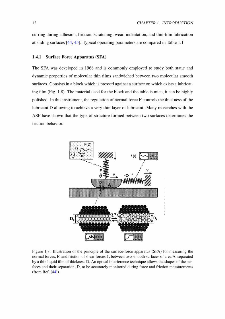
1.4.1 Surface Force Apparatus (SFA)
The SFA was developed in 1968 and is commonly employed to study both static and
dynamic properties of molecular thin films sandwiched between two molecular smooth
surfaces. Consists in a block which is pressed against a surface on which exists a lubricat-
ing film (Fig. 1.8). The material used for the block and the table is mica, it can be highly
polished. In this instrument, the regulation of normal force F controls the thickness of the
lubricant D allowing to achieve a very thin layer of lubricant. Many researches with the
ASF have shown that the type of structure formed between two surfaces determines the
friction behavior.
Figure 1.8: Illustration of the principle of the surface-force apparatus (SFA) for measuring thenormal forces, F, and friction of shear forces f , between two smooth surfaces of area A, separatedby a thin liquid film of thickness D. An optical interference technique allows the shapes of the sur-faces and their separation, D, to be accurately monitored during force and friction measurements(from Ref. [44]).

1.4. EXPERIMENTAL TECHNIQUES 13
1.4.2 Scanning Tunneling Microscopes (STM)
The Scanning tunneling microscope was invented by Gerd Binnig and Heinrich Rohrer of
IBM’s Zurich in 1981 and was the first instrument capable of generating actual images of
surfaces with atomic resolution. In 1986 its inventors won the Nobel Prize in Physics [46].
The microscope allows to get atomic resolution of electrically conductive surfaces and has
been used to clean surfaces pictures as well as of lubricant molecules [45]. According to
Fig. 1.9, the STM is composed of a thin needle coupled to a piezoelectric crystal. This
crystal has the ability to generate voltage in response to mechanical pressure. Thus, a
potential difference is applied between the needle and the material analyzed. When the
tip is placed very close to the sample surface in nanometer-scale approach, the sample
surface of the electrons begin to tunnel to the tip of the needle and vice-versa, depending
on the applied voltage polarity. When this happens, the tunneled electrons emit a small
electrical current (tunneling current). By measuring this electric current, we obtain a
topographic image of the surface with an atomic resolution.
Figure 1.9: Diagram of the Scanning Tunneling Microscope

14 CHAPTER 1. INTRODUCTION
1.4.3 Atomic Force and Friction Force Microscopes (AFM/FFM)
From a modification of the scanning tunneling microscope (STM), combined with a Sty-
lus profilometer (instrument to measure the roughness on a microscopic scale) Binnig,
Quate, and Gerber [47], developed the AFM in 1986. The experimental set-up of an
AFM/FFM is shown in Fig. 1.10; it is based on the so-called laser beam deflection method.
Cantilever deflection (i.e. normal force) and torsion (friction) of the cantilever are mea-
sured simultaneously by detecting the lateral and vertical deflections of a laser beam while
the sample is scanned in the x–y-plane. The laser beam deflection is determined using a
four-quadrant photo diode: if A, B, C and D are proportional to the intensity of the inci-
dent light of the corresponding quadrant, the signal (A + B)-(C + D) is a measure for the
deflection and (A +C)-(B + D) a measure for the torsion of the cantilever. A schematic
of the feedback system is shown by solid lines. The actual deflection signal of the photo
diode is compared with the set point chosen by the experimentalist. The resulting error
signal is fed into the PID controller (’PID’ stands for a feedback electronics that uses
a proportional, an integral, and a differential control part), which moves the z-position
of the scanner in order to minimize the deflection signal. Thanks to the FFM measure-
Figure 1.10: Experimental set-up of an AFM/FFM based on the laser beam deflection method(from Ref. [41]).
ment, it was revealed t,0hat the friction laws for a single asperity are different from the
macroscopic friction laws. The main result, confirmed by several experiments is that
the frictional force at the nanoscale shows a sawtooth behavior, often known as atomic
stick-slip [37]. This phenomenon can be reproduced by means of models of classical
1.4. EXPERIMENTAL TECHNIQUES 15
mechanics [13, 14, 48, 49, 50].
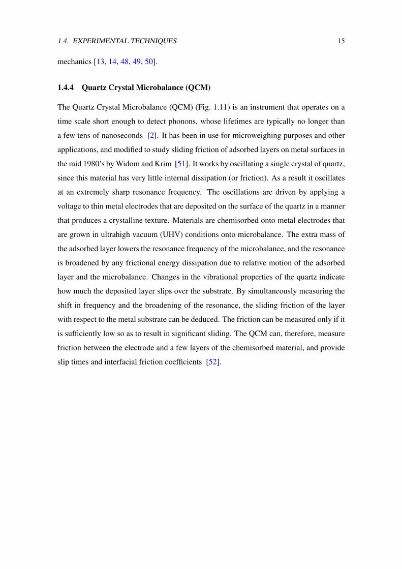
1.4.4 Quartz Crystal Microbalance (QCM)
The Quartz Crystal Microbalance (QCM) (Fig. 1.11) is an instrument that operates on a
time scale short enough to detect phonons, whose lifetimes are typically no longer than
a few tens of nanoseconds [2]. It has been in use for microweighing purposes and other
applications, and modified to study sliding friction of adsorbed layers on metal surfaces in
the mid 1980’s by Widom and Krim [51]. It works by oscillating a single crystal of quartz,
since this material has very little internal dissipation (or friction). As a result it oscillates
at an extremely sharp resonance frequency. The oscillations are driven by applying a
voltage to thin metal electrodes that are deposited on the surface of the quartz in a manner
that produces a crystalline texture. Materials are chemisorbed onto metal electrodes that
are grown in ultrahigh vacuum (UHV) conditions onto microbalance. The extra mass of
the adsorbed layer lowers the resonance frequency of the microbalance, and the resonance
is broadened by any frictional energy dissipation due to relative motion of the adsorbed
layer and the microbalance. Changes in the vibrational properties of the quartz indicate
how much the deposited layer slips over the substrate. By simultaneously measuring the
shift in frequency and the broadening of the resonance, the sliding friction of the layer
with respect to the metal substrate can be deduced. The friction can be measured only if it
is sufficiently low so as to result in significant sliding. The QCM can, therefore, measure
friction between the electrode and a few layers of the chemisorbed material, and provide
slip times and interfacial friction coefficients [52].

16 CHAPTER 1. INTRODUCTION
Figure 1.11: Front (a) and side (b) views of a QCM. The shaded regions represent metal electrodesthat are evaporated onto the major surfaces of the microbalance. Molecularly thin solid or liquidfilms adsorbed onto the surface of these electrodes (which are parallel to the x–z plane) depictedin (c) may exhibit measurable slippage at the electrode-film interface in response to the transverseshear oscillatory motion of the microbalance. The experiment is not unlike pulling a tableclothout from under a table setting, whereby the degree of slippage is deter- mined by the friction at theinterface between the dishes (i.e. the adsorbed film material) and the tablecloth (i.e. the surface ofthe electrode)(from Ref. [2]).

Chapter 2
Theoretical Foundations
A large variety of theoretical approaches have been adopted to study processes at surfaces
from a microscopic point of view [20]. The key goal of these approaches is to explain the
experimental findings and to predict new phenomena. In this regard, there are two ways
to approach the problem: trying to analyze atomic processes and structures in great detail
and keeping a close quantitative relation to real systems and experiments, or we can go for
“simple (minimalist) models”, based on simplified interatomic interactions and focus only
on the most relevant degrees of freedom of the system, trying to retain the most important
features. The advantage of the second approach is that they are computationally cheap
and simple enough to enable us to work out the general mechanisms of the problem, and
to provide a deeper physical understanding of the processes at play. These models can
explain phenomena of high complexity and allowed to make predictions which were later
verified experimentally.
2.1 Prandtl-Tomlinson Model
The development of experimental methods to investigate friction processes at the atomic
scale with numerical simulation methods announced a dramatic increase in the number of
studies in the area of friction between solids at the atomic scale.
One of the main results, confirmed by several experiments [53, 54], is that the friction
force on the nanometer scale exhibits a saw-tooth behavior, commonly known as “stick-
slip” motion. This observation can be theoretically reproduced within classical mechanics
using the Prandtl-Tomlinson model [14].
17

18 CHAPTER 2. THEORETICAL FOUNDATIONS
Over many years, this model has been referred as the “Tomlinson model" even though
the paper by Tomlinson did not contain it. In fact, it was Ludwing Prandtl who suggested
in 1928 a simple model for describing plastic deformation in crystals [13]. His contribu-
tions were more associated with fluid mechanics [55], mechanics of plastic deformations,
friction, and fracture mechanics [56]. In order to correct this historical error, in 2003
Müser, Urbakh, and Robbins, published a fundamental paper [57] in which the mentioned
model was termed “Prandtl-Tomlinson Model" [58]. Indeed, the Prandtl-Tomlinson (PT)
model has received some renewed attention, as can be seen for example in modeling the
aging effect on friction at the atomistic scale [59]. On the other side, Makkonen [3],
using a phenomenological thermodynamic approach, connected microscopic quantities
obtained by means of AFM, like the adhesion surface energy, with the macroscopic dry
friction coefficient. Although the approach seems very promising in predicting real mate-
rials coefficients, it does not provide a microscopic explanation of friction.
The model can explain the occurrence of static and kinetic friction, the origin of the
stick-slip behavior observed in the experiments and the transition to sliding states. It has
been successfully used to describe the movement of the tip and to model the scanning
process in AFM [60, 61, 62]. Here, we illustrate the properties of this model and its
extraordinary versatility to capture the nonlinear nature of frictional dynamics. Consider
the Prandtl-Tomlinson model in one dimension and at temperature T = 0. A cantilever
tip of mass m interacts with the surface via a periodic potential VTS and is attached by a
spring of elastic constant K to a support (cantilever) moving at constant velocity vc along
the x direction (see the sketch in Fig. 2.1).
For the 1D case we choose VTS of the form:
VTS(x) = U0[1− cos(2πx/a)] (2.1)
where a is the lattice constant of the substrate. The elastic interaction between the tip
and the support is
Vel(x) =1
2k(x− xs)2 (2.2)
where the support position xs is
xs = vct (2.3)

2.1. PRANDTL-TOMLINSON MODEL 19
vc t
a
m,k
2U0
Figure 2.1: Sketch of the 1D Prandtl-Tomlinson model for atomistic friction. The cantilever tip ofmass m and constant k is moving at constant velocity vc. The surface is represented as a potentialwith corrugation U0 and period a
It is assumed that the tip is a point-like object, representing the average over many atoms
of the real tip-surface contact. Energy dissipation in this model is introduced by adding
a damping term proportional to the tip velocity in the equation of motion. Thus, the
equation of motion in 1D becomes
mx+mηx = −2πU0
asin(
2πx
a)− k(x− vct) (2.4)
The solution of Eq. 2.4 is periodic, with period na/vc [63]:
x(t+ na/vc) = x(t) + na, for integer n. (2.5)
Typically n = 1 for not too small η, while in the strongly underdamped regime the
periodicity of the solution can be an integer multiple of the lattice constant. All energy
dissipation during sliding —whether it is due to phonons or due to electronic excitations—
is considered by a simple damping term that is proportional to the sliding velocity. This
simplification of the atomic-scale energy dissipation process is justified by the assumption
that there is no energy dissipation if the tip sticks (x ≈ 0), but energy dissipation will
occur as soon as the tip moves [64, 65]. The damping η is often an unknown parameter
20 CHAPTER 2. THEORETICAL FOUNDATIONS
in experiments and thus one has to adopt an ad hoc choice. Usually a critical damping,
η = 2√k/m [62] is assumed in order to reduce the oscillations of the tip and to avoid
multiple jumps. The underdamped regime is, however, characterized by a very complex
dynamical behavior [63]. The character of the motion in the Prandtl-Tomlinson model
crucially depends on the interplay between the tip-substrate potential (Eq. 2.1) and the
elastic potential (Eq. 2.2), or more specifically on the value of the cantilever stiffness k
and of the surface corrugationU0. The main mechanism of energy dissipation in the model
is determined by these elastic instabilities, and therefore we expect a more pronounced
contribution to kinetic friction in the stick-slip regime. The lateralforceFx to move the
tip in the x direction can be calculated from
Fx = k(vct− x) (2.6)
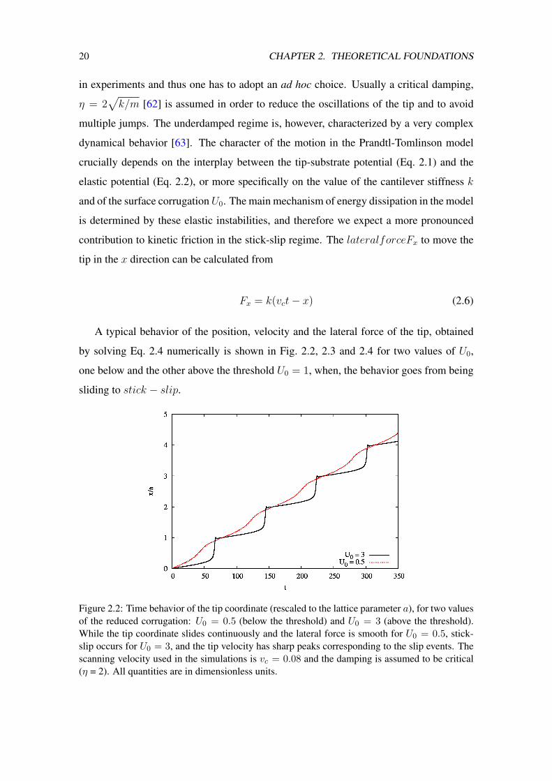
A typical behavior of the position, velocity and the lateral force of the tip, obtained
by solving Eq. 2.4 numerically is shown in Fig. 2.2, 2.3 and 2.4 for two values of U0,
one below and the other above the threshold U0 = 1, when, the behavior goes from being
sliding to stick − slip.
Figure 2.2: Time behavior of the tip coordinate (rescaled to the lattice parameter a), for two valuesof the reduced corrugation: U0 = 0.5 (below the threshold) and U0 = 3 (above the threshold).While the tip coordinate slides continuously and the lateral force is smooth for U0 = 0.5, stick-slip occurs for U0 = 3, and the tip velocity has sharp peaks corresponding to the slip events. Thescanning velocity used in the simulations is vc = 0.08 and the damping is assumed to be critical(η = 2). All quantities are in dimensionless units.

2.1. PRANDTL-TOMLINSON MODEL 21
Figure 2.3: Time behavior of the tip velocity for the same conditions as Fig. 2.2.
Figure 2.4: Time behavior of the lateral force for the same conditions as Fig. 2.2.

22 CHAPTER 2. THEORETICAL FOUNDATIONS
As can be seen in Fig. 2.5 and 2.6, the dynamics of the Prandtl-Tomlinson model
is very sensitive to the choice of the damping: when η = 0 there are many oscillations
with different frequencies. Whereas in the damped case, the behavior is smoother. The
parameter U0 is which regulates the transition between the sliding motion and stick-slip
and thus between high and low friction.
Figure 2.5: Comparison of the tip coordinate (rescaled to the lattice parameter a) for the undampedand the critically damped case, for U0 = 3. The cantilever scanning velocity is vc = 0.08. Allquantities are in dimensionless units.
Figure 2.6: Comparison of the lateral force (rescaled to the lattice parameter a) for the undampedand the critically damped case, for U0 = 3. The cantilever scanning velocity is vc = 0.08. Allquantities are in dimensionless units.
A work carried out by Socoliuc [66] using this model (Fig. 2.7) shows the comparison

2.1. PRANDTL-TOMLINSON MODEL 23
between experimental results for different loads values compared to simulations of Eq. 2.6
for different values of U0 (effective corrugation). The qualitative behavior is the same,
and interestingly, the behavior of the stick-slip movement and its hysteresis becomes less
evident as the load U0 decreases. These results are very significant, because they suggest
a way to control the friction in nanoscale without the use of lubricants, emphasize the
strength of the Prandtl-Tomlinson model in the description of dynamic friction.
Figure 2.7: Lateral force as a function of the tip position, as obtained by AFM experiments onNaCl(a-c) and by simulations of the Prandtl-Tomlinson model (d-f). The normal applied loads inthe experiments are Fload = 4.7nN (a), Fload = 3.3 (b) and Fload = −0.47 (c), while the valuesof U0 are U0 = 5 (d), U0 = 3 (e) and U0 = 1 (f). Notice the transition from stick-slip to slidingby decreasing the load in the experiments and by decreasing the effective corrugation U0 in thesimulations [66].
2.1.1 Velocity Dependence of Friction
As it was already mentioned in the introduction, the empirical laws of macroscopic fric-
tion cannot always be applied at the atomic level. One of them is the dependence of
friction with velocity. In this respect, several models and a varied of conclusions have
emerged and still controversy continues.
In the original experiments of Mate et al. [53] the authors observed that the frictional
force on a tungsten tip sliding on the basal plane of graphite for small loads shows little
dependence on velocity for scanning velocities up to 400 nm/s. On Zworner (1998) [64]
paper, the authors show the results of the velocity dependence of the friction at the contact

24 CHAPTER 2. THEORETICAL FOUNDATIONS
point between the tip and the substrate (Fig.2.8). The experimental results were obtained
using a frictional force microscope. It was found that the frictional forces are independent
of the sliding velocity, even in the nanometer scale for all sliding speeds performed, as
long as the sliding movement of the tip be faster than the sliding velocity.A similar behav-
ior has also been reported in the work of Zworner et al. [64] for velocities up to several
µm/s, where friction on different carbon structures has been studied. The authors of [64]
claim that a 1D Prandtl-Tomlinson model at T = 0 can reproduce a velocity independent
friction force for scanning velocities up to ∼ 1µm/s, while giving rise to linear increase
of friction for higher velocities. They conclude that Ffric is nearly constant in this range
of low velocities. With increasing sliding velocity, the frictional force is just proportional
to vc owing to the viscous damping Ffric ∼ γxvc which is indicated by the dashed line.
1
10
100
0.01 0.1 1 10 100 1000
Ffr
ic [
nN
]
vc [µm/s]
Zworner et al.2.25 + 0.06325vcγx vc
Figure 2.8: Data extracted from Zworner et al. [64] showing the frictional force (Ffric) as a func-tion of the sliding velocity (vc), along with the analytic expressions of the two limiting regimes.
Other works claim a logarithmic increase in the friction force with velocity, attributed
to thermal activation [67, 71, 37, 72, 73, 74, 75]. Fusco and Fasolino [20] have shown
that an appreciable velocity dependence of the friction force, for small scanning velocities
(from 1 nm/s to 1µm/s), is inherent to the Prandtl-Tomlinson model, having the form of
a power-law Ffric − F0 ∝ v2/3c . (Figure 2.9)
Depending on the investigated systems and/or models, on the simulation techniques
and/or conditions, different and somewhat contradictory results have been found on this
subject [20], even when using the same model.

2.2. THE FRENKEL-KONTOROVA MODEL 25
2.2
2.4
2.6
2.8
3
0 1 2 3 4 5 6 7 8
Ffr
ic [nN
]
vc [µm/s]
Simulation from Fusco et al.
Theory from Fusco et al.
1
10
0.0001 0.001 0.01 0.1 1 10
Ffr
ic [nN
]
vc [µm/s]
Simulation from Fusco et al.
Theory from Fusco et al.
Figure 2.9: Data extracted from Fusco and Fasolino [20] showing the friction force (Ffric) as afunction of the sliding velocity (vc), plotted on a linear (top) and on a log-log scale(bottom), in thesame way it was presented in the original article.
2.2 The Frenkel-Kontorova Model
The Frenkel-Kontorova model is one of the most simplest and rich models in classical me-
chanics. Involves a system shown in Fig. 2.10 where a one-dimensional chain of atoms
connected by springs of average length a interact with a harmonic potential in period b
[15]. The model was introduced at first to study dislocation in crystals, but it soon proved
useful in studying the mechanism of friction such as the origin of static friction and ef-
fect of structural commensurability. The simplicity of the model, due to the assumptions
of the harmonic interatomic force and sinusoidal on-site (substrate) potential, as well as
its surprising capability to describe a broad spectrum of nonlinear, physically important
phenomena, such as propagation of charge – density waves, the dynamics of absorbed
layers of atoms on crystal surfaces, commensurable–incommensurable phase transitions,
domain walls in magnetically ordered structures, etc., have attracted a great deal of at-
tention from physicists working in solid state physics and nonlinear physics [76]. One of
the important features which can explain why the FK model has attracted much attention
in different branches of solid state physics is the fact that in the continuum-limit approx-
imation the model reduces to the exactly integrable sine-Gordon (SG) equation which
possesses nice properties and allows exact solutions describing different types of nonlin-
ear waves and their interaction. In particular, the SG equation gives us an example of a
fundamental nonlinear model for which we know almost everything about the dynamics
of nonlinear excitations. As is known, the SG system describes simultaneously three dif-
ferent types of elementary excitations, namely phonons, kinks (topological solitons), and

26 CHAPTER 2. THEORETICAL FOUNDATIONS
breathers (dynamical solitons), whose dynamics determines the general behavior of the
system as a whole. And, although the FK model is inherently discrete and not exactly
integrable, one may get deep physical insights and significantly simplify the understand-
ing of its nonlinear dynamics using the language of the SG quasi-particles as weakly
interacting nonlinear excitations. Discreteness of the FK model manifests itself in such
a phenomenon as the effective periodic potential, known as the Peierls—Nabarro relief,
affecting the quasi-particle motion.
Figure 2.10: Schematic of the Frenkel-Kontorova model.
The dimensionless equation of motion for the atomic chain can be written as
xj + γxj = (xj+1 − 2xj + xj−1)− λsin2πxj + F (2.7)
with j = 1, 2, ..., N and xj is the position of the jth atom, γ denotes the internal damp-
ing coefficient in the atomic chain, λ = V/k represents a normalized potential strength
equal to the magnitude of the sinusoidal potential divided by the spring stiffness k, and F
is an external driving force. The contour conditions are:
xj+N = xj + 2πM
where M is an integer number. This conditions imply that the mean of the particles density
1/c is constant:
c = 2πM
N(2.8)
because of the symmetry, c is restricted to [0, π]. Several studies were carried out
using the above equation and friction as the focus, among them: in the super-damped

2.2. THE FRENKEL-KONTOROVA MODEL 27
regime for large N [77, 78, 79], at the limit with damping and external force equal to zero
[80]; in the sub-damping regime for small N [81, 82]; in the generalized under-damped
regime with large N and c near 0 and π [83]. But the most relevant fundamental work is
that of Strunz and Elmer [84]. This work differs only in the fact that c is not restricted
to any value in relation to the values studied in [83]. They find that Eq. 2.7 has stable
and unstable solutions, describing respectively two types of regular slip states: uniform
slip states and non-uniform slip states. Fig. 2.11 shows these states. The force versus
velocity characteristic curve shows stable and unstable solutions. Macroscopically, this
curve would have linear character of type F = γv. However, resonance of the chain of ad-
atoms for certain speeds of sliding results in the formation of phonons and consequently
peaks in the characteristic curve
Figure 2.11: Velocity-force characteristic. Solid (dotted) lines indicate stable (unstable) solutions.The smaller graph represents analytic solutions found. Arrows indicate resonant peaks, fromRef. [84].
The model was widely used to answer issues like how the energy dissipates on the
substrate, which is the main dissipation channel (electronic or phononic), and how the
phononic sliding friction coefficient depends on the corrugation amplitude [85, 86, 87].
In the work of [25], the authors used the FK model of an adsorbate-substrate interface to

28 CHAPTER 2. THEORETICAL FOUNDATIONS
calculate the phononic friction coefficient. They investigated the system, for different sub-
strate/adsorbate commensuration ratios in order to address how the phononic friction (and
therefore the sliding friction) depends on the commensuration ratio between substrate and
adsorbate. And demonstrate that the phononic friction coefficient depends quadratically
Figure 2.12: Total friction coefficient from different commensuration ratios (from Ref. [25])
on the substrate corrugation amplitude, but is a nontrivial function of the commensuration
ratio between substrate and adsorbate (Fig. 2.12).
In reference to this last subject, and from a experimental point of view, a recent work
was published [88] where the authors investigate the isotopic role on the dissipative
forces acting at the nanoscale in order to overcome the problem of the surface coverage
ratio effect on the friction phenomenon.
They discuss the issue of friction between a diamond spherical dome sliding on amor-
2.2. THE FRENKEL-KONTOROVA MODEL 29
phous carbon thin films containing different amounts of deuterium and/or hydrogen that
modifies the phonon-only distribution. Being more specific, the experimental results take
into account the physical contact under pressure arising between two sliding surfaces in
relative motion. They show that the friction coefficient decreases by substituting hydro-
gen by deuterium atoms. This result is consistent with an energy dissipation vibration
local mechanism from a disordered distribution of bond terminators.

30 CHAPTER 2. THEORETICAL FOUNDATIONS
Chapter 3
Models and Methods
In this work, in addition to explore the Prandtl-Tomlinson Model to analyze the depen-
dence of the friction with velocity, two one-dimensional models were proposed to rep-
resent the interaction between a substrate and a AFM microscope tip. In both cases, the
substrate is represented by independent harmonic oscillators. In the first model only two
particles are considered and in the second the substrate is represented by a chain of par-
ticles. The interaction between the tip and the substrate is a short-range Gaussian type
potential. In no case is any type of "ad-hoc" dissipation considered.
3.1 First Model: Energy exchange in a two particles system
The first model consists of two particles: a mass that is thrown to move past another one,
which is attached to a spring (Fig. 3.1). The interaction between the particles is nonlinear
and short-ranged. For simplicity, the motion is considered in one dimension, but the free
particle can overcome the bound one because the interaction potential between them has
a finite maximum. This seemingly unreal situation is a simplified model of a particle
sliding on top of another, where the transverse movement is not taken into account. The
asperity is represented by a single free particle and the substrate by a harmonic oscillator.
As shown in Fig. 3.1 the free particle is impelled from a region where it is not affected by
the presence of the oscillator, until eventually it interacts with it. This local interaction is
repulsive, short ranged, and with a finite maximum; for simplicity a Gaussian is used for
the interaction potential.
31

32 CHAPTER 3. MODELS AND METHODS
vf
mf
ma
k
U0
Figure 3.1: Schematic representation of the two particle model.
Therefore the proposed model is represented by the Hamiltonian
H =p2f
2mf
+p2a
2ma
+1
2maω
2x2a + U(xf , xa) (3.1)
where pf , xf , pa, xa are the momentum and position of the free particle and the oscillator
respectively. The masses of the two are unequal and represented by mf and ma respec-
tively. The oscillator frequency is ω =√k/ma, where k is the spring constant. As it was
said, the interaction potential U(|xf − xa|) is assumed to be a Gaussian with a maximum
value U0, the height of the potential, and a width σ, which characterizes the typical range
or length of the interaction. From the Hamiltonian in Eq. (3.1), the following equations
of motion are derived:
xf =
(2U0
mfσ2
)(xf − xa)e−
(xf−xa)2
σ2 (3.2)
xa = −ω2xa −(
2U0
maσ2
)(xf − xa)e−
(xf−xa)2
σ2 , (3.3)
which have five parameters. By defining dimensionless variables q = x/σ and τ =√U0
mfσ2 t, and writing the equations of motion in terms of them,

3.2. SECOND MODEL: PRANDTL-TOMLINSON MODEL IMPROVED WITH NO AD-HOC DISSIPATION33
qf = 2(qf − qa)e−(qf−qa)2
(3.4)
qa = −Γ2
µqa − 2
(qf − qa)µ
e−(qf−qa)2
, (3.5)
the number of free parameters can be reduced to two: the ratio of the masses of the two
objects (µ = mamf
), and a dimensionless oscillator frequency (Γ =√
kσ2
U0). It is therefore
important to understand the dynamics of the system in terms of the relative masses and
the frequency of the oscillator, which is addressed in the next section.
Working with Eqs. (3.2) and (3.3), the behavior of the system in terms of those two
parameters is characterized. It is worth to notice that the Gaussian potential was chosen
for no particular reason except for being simple an short ranged, capturing the essential
features of the interaction among the “substrate” and “adsorbate”. On the other side, it
makes the problem nonlinear with no close analytic solution.
3.2 Second Model: Prandtl-Tomlinson model improved with no ad-
hoc dissipation
The second model proposed and studied is an extension of the last model (Fig. 3.2), where
ms, ks are the masses of the substrate particles and their spring constants; mt, kt are the
tip mass and spring constant respectively. U0 is the height of the interaction potential and
ax is the lattice constant. The tip is driven by a support that moves at constant velocity vc .
The substrate is represented by a series of spring-masses, independent between them, but
interacting with the tip via a short range Gaussian type potential. To avoid edge effects
we modeled the chain as being sufficiently long.
The system is described by the Hamiltonian
H =P 2
2mt
+N∑i=1
p2i2ms
+N∑i=1
U(X, xi) + U(X) +N∑i=1
U(xsi) (3.6)
where X,P and x, p are the tip and substrate coordinates respectively; U(X, xi) =
U0e− (X−xi)
2
σ2 is the interaction between the tip and each of the particles of the substrate
and N is the number of particles. We choose the value of σ such that the potentials do not

34 CHAPTER 3. MODELS AND METHODS
vc
a
mt,kt
ms,ks
U0
Figure 3.2: Extension of the two particles interaction model to a N -particle model: ms and ksare the mass and spring constant of the substrate; mt , kt are the tip mass and spring constantrespectively. U0 is the height of the interaction potential and a is the lattice constant. The tip isdriven by a support that moves at constant velocity vc
overlap each other and the tip can interact with each of them separately: σ = ax/n, where
ax is the separation between the particles of the substrate and n a constant. U(X) =
kt2
(X − xc)2 is the elastic interaction between the tip and the cantilever. The support
position xc is xc = vct.And U(xi) = ks2
(xi − x0i)2 is the elastic potential of each particle
(independent between them). The energy dissipation can be added introducing a damping
term proportional to the tip velocity.
This results in the following equation of motion:
mtX = −kt(X − vct) +2U0
σ2
N∑i=1
(X − xi)e−(X−xi)
2
σ2 (3.7)
ms
N∑i=1
xi = −ksN∑i=1
(xi − x0i)−2U0
σ2
N∑i=1
(X − xi)e−(X−xi)
2
σ2 (3.8)
Introducing the dimensionless units Q = Xσ, q = x
σ, τ =
√ktmtt, U0 = 2U0
ktσ2 , vc =
vcσ
√mtkt
, the equations 3.7 and 3.8 can be reduced to:
3.3. MOLECULAR DYNAMICS 35
Q = −q + vcτ + U0
N∑i=1
(Q− qi)e−(qt−qsi )2
(3.9)
N∑i=1
qi =ε1ε2
N∑i=1
(qi − q0i)− ε1U0
N∑i=1
(Q− qi)e−(Q−qi)2
(3.10)
where ε1 = mt/ms is the ratio of the mass of the tip and the substrate particles (assuming
all have the same masses) and ε2 = kt/ks is the ratio of the stiffness of the tip and the
substrate.
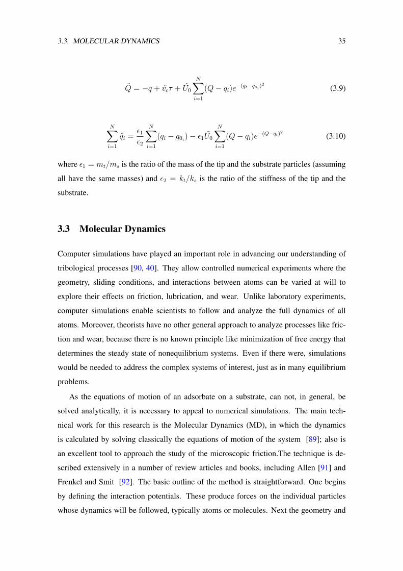
3.3 Molecular Dynamics
Computer simulations have played an important role in advancing our understanding of
tribological processes [90, 40]. They allow controlled numerical experiments where the
geometry, sliding conditions, and interactions between atoms can be varied at will to
explore their effects on friction, lubrication, and wear. Unlike laboratory experiments,
computer simulations enable scientists to follow and analyze the full dynamics of all
atoms. Moreover, theorists have no other general approach to analyze processes like fric-
tion and wear, because there is no known principle like minimization of free energy that
determines the steady state of nonequilibrium systems. Even if there were, simulations
would be needed to address the complex systems of interest, just as in many equilibrium
problems.
As the equations of motion of an adsorbate on a substrate, can not, in general, be
solved analytically, it is necessary to appeal to numerical simulations. The main tech-
nical work for this research is the Molecular Dynamics (MD), in which the dynamics
is calculated by solving classically the equations of motion of the system [89]; also is
an excellent tool to approach the study of the microscopic friction.The technique is de-
scribed extensively in a number of review articles and books, including Allen [91] and
Frenkel and Smit [92]. The basic outline of the method is straightforward. One begins
by defining the interaction potentials. These produce forces on the individual particles
whose dynamics will be followed, typically atoms or molecules. Next the geometry and

36 CHAPTER 3. MODELS AND METHODS
boundary conditions are specified, and initial coordinates and velocities are given to each
particle. Then the equations of motion for the particles are integrated numerically, step-
ping forward in time by discrete steps of size ∆t. Quantities such as forces, velocities,
work, heat flow, and correlation functions are calculated as functions of time to determine
their steady-state values and dynamic fluctuations. The relation between changes in these
quantities and the motion of individual molecules is also explored.
In this way, the temporal and spatial evolution of the adsorbate are calculated when
interact with the surface atoms. In MD, the form of potential energy is given explicitly as
a function of the position of atoms. Although the MD simulations can give very precise
results and are able to follow the dynamic details of the system, in most cases are limited
to short time scales (in the order of 100 ns) since the typical time interval is very tiny.
Several studies using this technique have been made in recent years [18] [24] [21] [25].
There are several ways to solve the equations numerically. Basically, we have to include
the stochastic forces on the algorithm used to solve deterministic equations, such as the
Verlet and Velocity Verlet algorithm, used in this work.
3.3.1 Verlet Algorithm
The numerical integration of the equations of motion is performed by algorithms based
on the finite difference method, in which the integration is divided into small time steps
(integration step) [93], ∆t, such as Velocity Verlet or Runge-Kutta [91, 92, 94, 95]. One
of the most used methods in molecular dynamics to integrate the equations of motion is
the Verlet algorithm, which uses the positions and accelerations of atoms at time t and the
previous step positions, r(t−∆t) to determine the new position at time t+ ∆t as we can
see from Eq. 3.11
r(t+ ∆t) = 2r(t)− r(t−∆t) +f(t)
m∆t2 (3.11)
This algorithm can be obtained through expanding in Taylor series, initially forward
(Eq. 3.12), and then backwards (Eq. 3.13). Adding the two equations and isolating r(t +
∆t), we get the Eq. 3.11 (9)
r(t+ ∆t) = r(t) + v(t)∆t+1
2
f(t)
m∆t2 + ... (3.12)

3.3. MOLECULAR DYNAMICS 37
r(t−∆t) = r(t)− v(t)∆t+1
2
f(t)
m∆t2 − ... (3.13)
The velocity is given by
v(t) =r(t+ ∆t)− r(t−∆t)
2∆t(3.14)
3.3.2 Velocity Verlet Algorithm
In our simulations we have employed the velocity Verlet algorithm, which, at variance
with the Runge-Kutta, is a symplectic algorithm (i.e. it retains many dynamical properties
of the phase space that the exact trajectories are known to exhibit), and thus it is more
robust and stable. The velocity Verlet algorithm computes the particle velocity v(t+ ∆t)
and the position r(t+ ∆t) at time t+ ∆tas follows:
r(t+ ∆t) = r(t) + v(t)∆(t) +F (t)∆t2
2m(3.15)
v(t+ ∆t) = v(t) +(F (t) + F (t+ ∆t))∆t
2m(3.16)
In the equations above, F (t) is the force at time t acting on the particle, which depends
only on the position x(t). The algorithm is self starting.

38 CHAPTER 3. MODELS AND METHODS

Chapter 4
Results and Discussions
This chapter is divided into three sections: the first one corresponds to the velocity-friction
dependence in the Prandtl-Tomlinson model [68]. The second section is dedicated to the
results of the first [69] model and the third to the results of the second model [70].
4.1 Prandtl-Tomlinson model revisited
Considering the variety of seemingly conflicted results, in this chapter we address this
apparent paradox in the Prandtl-Tomlinson model at zero temperature, studying the force-
velocity relation for a wide range of velocities not previously presented. Including much
more data density for the non trivial regions, we are able to shed light on this problem and
at the same time, provide new insight in the use of the paradigmatic Prandtl-Tomlinson
model for the secular problem of friction laws.
In this way we can show that depending on how the results are presented, it is possi-
ble to arrive to apparently different conclusions. However, taking the whole picture, the
results of the different contributions can be reconciled.
In Fig. 4.1 is shown the lateral force Fx; and tip velocity vt in Fig. 4.2 for different
sliding velocities using the model of Prandtl-Tomlinson. The values of the constants for
the model are: k = 10 N/m, m = 10−10 kg (which gives a natural frequency for the tip,√k/m ' 316 kHz), and a = 0.3 nm, typical values of AFM experiments [71, 62, 64, 20].
In general, the amplitude used for the corrugation U0 goes from 0.2 to 2 eV [72], and in the
present case we use U0 = 1 eV. We chose γ = 2√k/m in order to have critical damping,
39

40 CHAPTER 4. RESULTS AND DISCUSSIONS
and the time step used for the numerical integration was ∆t ' 1 ns 1. These particular
set of parameters were chosen in order to compare our results with those obtained by
Zworner et al. [64] and Fusco and Fasolino [20].
0
2
4
6
8
10
12
0 3 6 9 12 15 18 21
Fx
[nN
]
xc [(Å)]
vc = 0.001 µm/svc = 1 µm/s vc = 10 µm/s
vc = 100 µm/s
Figure 4.1: Lateral force Fx for different sliding velocities vc = 0.001µm/s to 10µm/s
If to each sliding velocity, we compute the average of the frictional force Ffric over
many stick-slip periods, we obtain the Friction force in function of the sliding velocity of
the cantilever.
With the help of the software Engauge Digitizer [96] we recover the data points from
the graphics of the mentioned references; in this way we can reproduce the plots of their
simulations in the most similar way to the original articles as it was shown on Fig. 2.9
This also allowed us to make graphics along with the results from our own simulations
(as shown in Fig. 4.3), so we can compare the three set of data in the different regions.
Our numerical results are extended down to 0.1 nm/s, in order to show that, in prin-
ciple, all data seems to be consistent. It can be appreciated from the plot in linear scale
(Fig. 4.3 left), that this consistency is hard to appreciate, particularly under 1µm/s where
many order of magnitude are condensed. For this reason, the same data has to be pre-
sented in a more convenient scale, which is the case of a semi-log scale (Fig. 4.3 right).1The period of oscillation of the cantilever is 20µs and the maximum simulated speed is 1mm/s, so that time step
is more that 1000 times smaller that the period and at the maximum speed it moves only 1/300 of the potential length
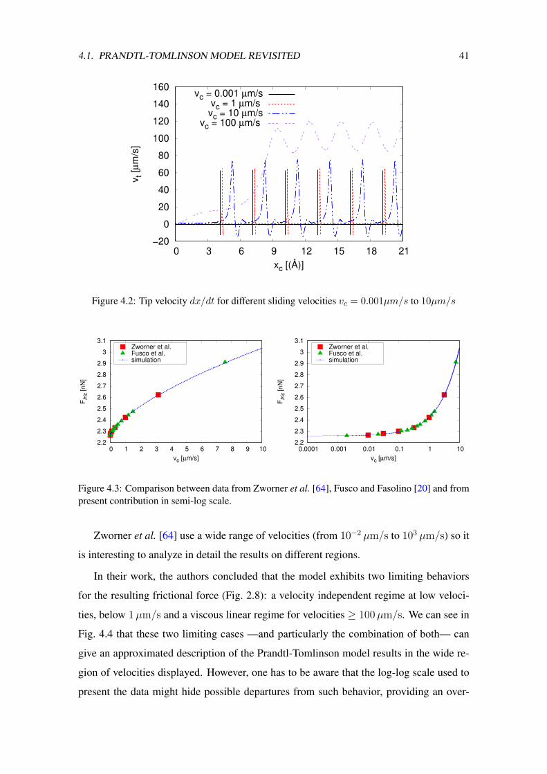
4.1. PRANDTL-TOMLINSON MODEL REVISITED 41
−20
0
20
40
60
80
100
120
140
160
0 3 6 9 12 15 18 21
v t [µ
m/s
]
xc [(Å)]
vc = 0.001 µm/svc = 1 µm/s vc = 10 µm/s
vc = 100 µm/s
Figure 4.2: Tip velocity dx/dt for different sliding velocities vc = 0.001µm/s to 10µm/s
2.2
2.3
2.4
2.5
2.6
2.7
2.8
2.9
3
3.1
0 1 2 3 4 5 6 7 8 9 10
Ffr
ic [
nN
]
vc [µm/s]
Zworner et al.Fusco et al.simulation
2.2
2.3
2.4
2.5
2.6
2.7
2.8
2.9
3
3.1
0.0001 0.001 0.01 0.1 1 10
Ffr
ic [
nN
]
vc [µm/s]
Zworner et al.Fusco et al.simulation
Figure 4.3: Comparison between data from Zworner et al. [64], Fusco and Fasolino [20] and frompresent contribution in semi-log scale.
Zworner et al. [64] use a wide range of velocities (from 10−2 µm/s to 103 µm/s) so it
is interesting to analyze in detail the results on different regions.
In their work, the authors concluded that the model exhibits two limiting behaviors
for the resulting frictional force (Fig. 2.8): a velocity independent regime at low veloci-
ties, below 1µm/s and a viscous linear regime for velocities ≥ 100µm/s. We can see in
Fig. 4.4 that these two limiting cases —and particularly the combination of both— can
give an approximated description of the Prandtl-Tomlinson model results in the wide re-
gion of velocities displayed. However, one has to be aware that the log-log scale used to
present the data might hide possible departures from such behavior, providing an over-
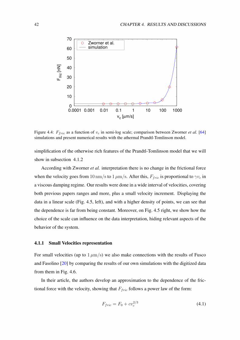
42 CHAPTER 4. RESULTS AND DISCUSSIONS
0
10
20
30
40
50
60
70
0.0001 0.001 0.01 0.1 1 10 100 1000
Ffr
ic [
nN
]
vc [µm/s]
Zworner et al.simulation
Figure 4.4: Ffric as a function of vc in semi-log scale; comparison between Zworner et al. [64]simulations and present numerical results with the athermal Prandtl-Tomlinson model.
simplification of the otherwise rich features of the Prandtl-Tomlinson model that we will
show in subsection 4.1.2
According with Zworner et al. interpretation there is no change in the frictional force
when the velocity goes from 10 nm/s to 1µm/s. After this, Ffric is proportional to γvc in
a viscous damping regime. Our results were done in a wide interval of velocities, covering
both previous papers ranges and more, plus a small velocity increment. Displaying the
data in a linear scale (Fig. 4.5, left), and with a higher density of points, we can see that
the dependence is far from being constant. Moreover, on Fig. 4.5 right, we show how the
choice of the scale can influence on the data interpretation, hiding relevant aspects of the
behavior of the system.
4.1.1 Small Velocities representation
For small velocities (up to 1µm/s) we also make connections with the results of Fusco
and Fasolino [20] by comparing the results of our own simulations with the digitized data
from them in Fig. 4.6.
In their article, the authors develop an approximation to the dependence of the fric-
tional force with the velocity, showing that Ffric follows a power law of the form:
Ffric = F0 + cv2/3c (4.1)

4.1. PRANDTL-TOMLINSON MODEL REVISITED 43
2.5
3
3.5
0 5 10 15 20 25 30 35 40 45 50
Ffr
ic [
nN
]
vc [µm/s]
Zworner et al.simulation
2.5
3
3.5
0.0001 0.001 0.01 0.1 1 10
Ffr
ic [
nN
]
vc [µm/s]
Zworner et al.simulation
Figure 4.5: Comparison between data from Zworner et al. [64] and from present contribution inlinear and semi-log scale.
where c is a constant that depends on the parameter of the model and on the space dimen-
sion. This approximation is very accurate for this range of velocities. Highlighting again
that the friction is not independent of the velocity. This proves that depending on the scale
chosen to represent the data, important information can be overlooked. The same Figure
also shows that this power-law dependency continues to be valid for higher velocities of
up to 20µm/s.
2.2
2.4
2.6
2.8
3
3.2
3.4
3.6
0.0001 0.001 0.01 0.1 1 10
Ffr
ic [nN
]
vc [µm/s]
Zworner et al.Fusco et al.simulationFfric − F0 ∝ vc
2/3
Figure 4.6: Increase of the frictional force with velocity between 10−3 µm/s to 20µm/s. The lineis a power-law fit to the data of the form Ffric − F0 ∝ v2/3c , from Ref. [20].
44 CHAPTER 4. RESULTS AND DISCUSSIONS
4.1.2 Transitional and Large Velocities representation
An important fact that stands out is the distinctive behavior in the region between 10µm/s
and 35µm/s (Fig. 4.9), where Ffric oscillates with vc around a fixed value of force. In-
deed, for the velocities vc in this region,the tip sees a force from the surface that varies
with the a frequency close to its own natural frequency [19, 97], i.e.:
vresc =a
2π
√k
m' 15µm/s (4.2)
In order to better understand what could be the origin of the reported behavior we
present below the tip position and velocity as a function of the cantilever position (Fig. 4.7
and Fig. 4.8). We present that data for different values of the sliding cantilever velocity.
For velocities well below the region where friction oscillates, we have the typical stick-
slip behavior where energy dissipates mainly after the slip movement. For large velocities
the viscous regime is recovered. However in the region of interest we observe that the tip
slips over a distance of two cell parameters, from one potential barrier to the second other
one. This happens only for a damping coefficient near critical. Then, instead of being
a resonance phenomenon, it is a critical damping effect where the dissipation remains at
its minimum compatible with the sliding speed (Fig. 4.8). The presence of double jumps
for that range of velocities, makes us to wonder if multiple (more than two) slide jumps
would be possible. That can happen, depending on the key parameters of the model, i.e.,
U0, k, and a [98], and it deserves a future and thorough analysis.
Such behavior comes to light in reason of the remarkable increase in the density of
simulated points and it has not been reported before. In this segment the value of Ffric os-
cillates around an average value of 3.35 nN. This behavior goes totally unnoticed in a log-
arithmic representation of the data. Some recent experiments [104, 99] have been carried
out evaluating the friction dependence on speed near this region, but without covering the
entire range and without sufficient detail and precision. In the work of Gangloff [105],the
authors also find a similar behavior that they call a friction plateau between between
10−3 and 10−2 m/s and four regimes of friction for an ion-crystal system. The difference
with our numerical results is mostly due to the choice of parameters in this contribution.
After the transition region, we observe that friction growths again. We fit the data with

4.1. PRANDTL-TOMLINSON MODEL REVISITED 45
0
3
6
9
12
15
18
21
24
0 3 6 9 12 15 18 21
x t [
µm
/s]
xM [(Å)]
vM = 1 µm/s vM = 20 µm/svM = 50 µm/s
Figure 4.7: Tip position as a function of cantilever position for different sliding velocities, before,at, and after the region where friction oscillates.
−50
0
50
100
150
0 3 6 9 12 15 18 21
v t [
µm
/s]
xM [(Å)]
vM = 1 µm/s vM = 20 µm/svM = 50 µm/s
Figure 4.8: Tip velocity as a function of cantilever position for different sliding velocities, before,at, and after the region where friction oscillates.
a quadratic power-law:
Ffric − F ∝ v2c (4.3)
where F is the value of the friction at the lower velocity of the adjustment (Fig. 4.10). The
quadratic growth fits very well with the simulation data up to 0.1 mm/s behaving like a
drag force until finally, for large sliding velocities, the mechanism of energy dissipation

46 CHAPTER 4. RESULTS AND DISCUSSIONS
3.2
3.4
3.6
15 20 25 30 35
Ffr
ic [
nN
]
vc [µm/s]
Standard deviation = 0.045mean = 3.35simulation
Figure 4.9: Detail of the behavior of the friction force with velocity between 15 to 35µm/s. Wecan say that friction is stationary in this range of velocities.
through the “stick-slip” effect breaks down, and Ffric is proportional to γvc, where critical
damping is assumed, giving γ = 2√km.
10
100
Ffr
ic [
nN
]
vc [µm/s]
simulationFfric − F0 ∝ vc
2/3
Ffric − F1 ∝ vc2
γ vcFfric = 3.34
Figure 4.10: The friction force as a function of velocity in the transition region between the lowvelocities v2/3c regime to the high velocities, viscous linear regime. For that intermediate regimeof velocities the force goes through two other transitional regimes of almost constant force toquadratic velocity regime before entering the linear regime. Increase of the frictional force withvelocity between 35 to 100µm/s. The line is a power-law fit to the data of the form Ffric − F ∝v2c . For high velocities the frictional force is proportional to the velocity in the regime of viscousdamping

4.2. TWO PARTICLES INTERACTION 47
4.2 Two particles interaction
4.2.1 Non Oscillator
First, a non-oscillator or a free particle is consider. By setting k = 0 and defining x =
xf − xa and X =mfxf+maxamf+ma
as the internal and center of mass coordinate respectively in
Eqs. (3.2) and (3.3), the following equations are obtained:
x =
(2U0
σ2
)(1
mf
+1
ma
)xe−x
2/σ2
(4.4)
X = 0 . (4.5)
Eqs. (4.4) and (4.5) can also be written in terms of conserved quantities as
x2
2+ U0
(1
mf
+1
ma
)e−x
2/σ2
=v202
(4.6)
X(t) = X(0) = − v0mf
mf +ma
, (4.7)
where it is assumed that the two particles are initially well apart from each other, that
the free particle starts with velocity −v0 (v0 > 0) moving to the bound mass, which is
initially in equilibrium at rest. With these initial conditions it is straightforward to derive
the asymptotic relation between the velocities, when one of the particles has gone far away
from the interaction region, i.e., the potential term goes to zero, so from Eq. (4.6-4.7) the
next relations are obtained:
vf (∞)− va(∞) = ±v0 (4.8)
vf (∞) +ma
mf
va(∞) = −v0 . (4.9)
Combining Eq. (4.8-4.9), the minus sign solution gives va(∞) = 0 and vf (∞) = −v0 =
vf (0), so the incoming particle passes through the fixed one, moving away with the same
asymptotic velocity it had initially, while the bound one stays at rest after the interaction.
Such asymptotic situation, in which the incoming particle does not loose energy after the
interaction, happens whenever the initial kinetic energy of the incoming particle is larger

48 CHAPTER 4. RESULTS AND DISCUSSIONS
than the maximum of the interaction potential energy, i.e:
|vf (0)| > vcr =
√2U0
(1
mf
+1
ma
). (4.10)
The plus sign in Eq. (4.8) gives va(∞) =(
2mfmf+ma
)vf (0) and vf (∞) =
(mf−mamf+ma
)vf (0)
as solutions. Therefore, vf (∞) can be positive, zero, or negative depending on the relation
of the two masses. However, in any case the velocity of ma is always bigger than the
velocity of mf , meaning that the free particle can not overcome the other when |vf (0)| <
vcr. This is the well-known case of elastic collision which, in the center of mass reference
system, has a unified description for the three cases, and as such has no relation with the
friction related problem we address here. Figure 4.11 shows the final velocity of the free
particle as a function of its initial velocity for the case ma/mf = 2.
-1.5
-1
-0.5
0
0.5
1
-1.5 -1 -0.5
(vf (∞
) -
va(∞
))/
vcr
vf (0)/vcr
Figure 4.11: Final velocity of the incoming particle, vf (∞)/vcr, as a function of its initial velocity,vf (0)/vcr (both in terms of the critical velocity) for the k = 0 case. The dashed lines showsthe analytic expression and the solid lines are obtained from numerical simulations. The otherparameters of the system are U0 = 1 and σ = 1, ma is initially at rest (va(0) = 0) and far fromthe incoming mf particle (vf (0) = −v0 < 0).
4.2.2 Oscillator
The relationship between the initial and final velocities, described before for the case
k = 0, can become quite complex for k > 0, when the second particle is bound to the

4.2. TWO PARTICLES INTERACTION 49
equilibrium position of the harmonic potential. In Fig. 4.12 it is shown the dependence of
the final velocity of the free particle (mf ) after interacting with the bound particle for three
different mass ratios: mamf
= 2, 1, and 0.5. Different behaviors are observed depending
also on the spring constant k being soft, or intermediate.

50 CHAPTER 4. RESULTS AND DISCUSSIONS
-1.5
-1
-0.5
0
0.5
1
-1.5 -1 -0.5
ma/mf = 2
vf (∞
) /
vcr
vf (0)/vcr
k = 0k = 0.1k =1k = 5
-1.5
-1
-0.5
0
0.5
1
-1.5 -1 -0.5
ma/mf = 1
vf (∞
) /
vcr
vf (0)/vcr
k = 0k = 0.1k = 1k = 5
-1.5
-1
-0.5
0
0.5
1
-1.5 -1 -0.5
ma/mf = 0.5
vf (∞
) /
vcr
vf (0)/vcr
k = 0k = 0.005k = 0.5k = 5
Figure 4.12: Final velocity of the incoming particle, vf (∞)/vcr, as a function of its initial velocity,vf (0)/vcr (both in terms of the critical velocity) for the (k 6= 0) case. The other parameters of thesystem are U0 = 1 and σ = 1, ma is initially at rest (va(0) = 0) and far from the incoming mf
particle (vf (0) = −v0 < 0). Solid (blue) lines show correspond to (k = 0) cases non and havebeen drawn for reference.

4.2. TWO PARTICLES INTERACTION 51
Generally, for large velocities, the free particle overcomes the bound particle with
almost no loss of energy, and for low velocities it bounces back, losing some energy which
depends on the mass ratio, the value of k, and the initial velocity. Both these situations
are not of much interest because they have no implications on the friction problem. Rich
and non trivial behavior is observed in the intermediate velocity range, between the k = 0
critical velocity and the k > 0 critical velocity (which also depends on the mass ratio).
Looking at the upper and central panels of Fig. 4.12, it can be seen that the behavior
in the intermediate range of velocities is qualitative similar for different mass ratios, the
critical velocity shifts to lower values of |v| as k increases and the energy loss increases
with k too. The shift of the critical velocity to lower values when k increases is expected
because in the limit of k →∞ it is recovered the trivial case of fixed potential, with a crit-
ical velocity determined by the height of the potential. Let us mention that such extreme
case, is of no interest too, because there is no emerging “friction” due to conservation of
energy of the mf particle. Therefore, the exchange of energy between the free and the
bound particle is expected to show a maximum at some intermediate k value, as can be
seen in Fig. 4.13, which depends on the mass ratio.
0.7
0.8
0.9
1
0 5 10 15 20 25 30 35 40
Ef/E
i
k
ma/mf = 0.5
ma/mf = 1
ma/mf = 2
Figure 4.13: Energy ratio vs k for three different mass ratios. The initial velocity of the freeparticle is |vf (0)| = 2.
Another general behavior observed in Fig. 4.12 is that as the free mass (mf ) increases,
relative to the bound mass, the change in the critical velocity becomes more sensitive to
the stiffness of the bound particle, k. More precisely, the shift as a function of k is more
52 CHAPTER 4. RESULTS AND DISCUSSIONS
dramatic for larger value of the mass mf . A peculiar situation is observed when the free
particle is more massive than the bound one (Fig. 4.12 lower panel), where a complex
behavior, with more that one critical velocity, is observed for intermediate values of k.
Such a case is discussed in the next section.
4.2.3 Soft k (slow oscillations)
We focus here on the case of soft k which results in slow oscillations of the bound particle.
The lower panel of Fig. 4.12 (ma/mf = 0.5) displays a small window in the initial
velocity in which the free particle gets transmitted with a significant loss of energy to
the oscillator. Beyond this window the free particle is reflected back. As can be seen in
Fig. 4.14 the transition between transmission and reflection exhibits sensitive dependence
on the initial conditions. That is, for initial velocities which differ in less than 1 in 104,
the free particle changes from reflection to transmission. Moreover, the free particle is
seen to reflect back with almost the same incoming energy (blue curves in Fig. 4.14). For
a slightly larger initial velocity, the free particle is transmitted with less energy than it
had initially (red curves in Fig. 4.14). Therefore, in the latter case, much of the energy is
transferred into the oscillatory mode of the bound particle. In both situations, however,
the two particles interact twice. Such behavior is observed over a range of parameter
values.
Since the two collisions are well separated in time, the analysis of the previous section
for k = 0 can be extended to the two collision observed here for k ≈ 0. The approxima-
tion considers that the two particles move independently (mf moves at constant velocity
and ma is subject to the harmonic potential) except at the collisions, when the results of
the previous section for free particles are applied.
Since the initial velocity of the free particle is less than the critical velocity (vcr)
defined in Eq. (4.10), immediately after the first collision (t > t1) the velocities are:
vf (t+1 ) =
mf −ma
mf +ma
vf (0) (4.11)
va(t+1 ) =
2mf
mf +ma
vf (0) , (4.12)
where, t∓i denote the time immediately before and after the collision. Assuming that after
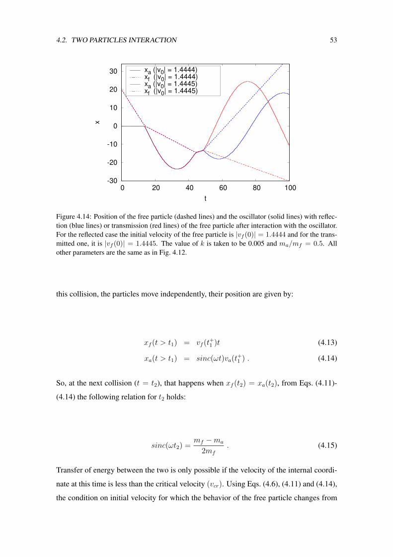
4.2. TWO PARTICLES INTERACTION 53
-30
-20
-10
0
10
20
30
0 20 40 60 80 100
x
t
xa (|v0| = 1.4444)xf (|v0| = 1.4444)xa (|v0| = 1.4445)xf (|v0| = 1.4445)
Figure 4.14: Position of the free particle (dashed lines) and the oscillator (solid lines) with reflec-tion (blue lines) or transmission (red lines) of the free particle after interaction with the oscillator.For the reflected case the initial velocity of the free particle is |vf (0)| = 1.4444 and for the trans-mitted one, it is |vf (0)| = 1.4445. The value of k is taken to be 0.005 and ma/mf = 0.5. Allother parameters are the same as in Fig. 4.12.
this collision, the particles move independently, their position are given by:
xf (t > t1) = vf (t+1 )t (4.13)
xa(t > t1) = sinc(ωt)va(t+1 ) . (4.14)
So, at the next collision (t = t2), that happens when xf (t2) = xa(t2), from Eqs. (4.11)-
(4.14) the following relation for t2 holds:
sinc(ωt2) =mf −ma
2mf
. (4.15)
Transfer of energy between the two is only possible if the velocity of the internal coordi-
nate at this time is less than the critical velocity (vcr). Using Eqs. (4.6), (4.11) and (4.14),
the condition on initial velocity for which the behavior of the free particle changes from

54 CHAPTER 4. RESULTS AND DISCUSSIONS
transmission to reflection is
vf (0) =vcr(mf +ma)
mf (1− 2 cos(ωt2))−ma
. (4.16)
The instantaneous velocity after the second collision can be obtained from conservation
of energy and momentum and is given by
vf (t+2 ) =
2ma
ma +mf
va(t−2 ) +
mf −ma
ma +mf
vf (t−2 ) (4.17)
va(t+2 ) =
ma −mf
ma +mf
va(t−2 ) +
2mf
ma +mf
vf (t−2 ) . (4.18)
Figure 4.15 shows a comparison between the approximate two collision theory and nu-
merical results forma/mf = 0.5 and k = 0.005. For these parameter values, the different
behaviors in the final velocity are distinctly observed and the two collision approximation
is able to provide an excellent fit to the numerical results. There is another critical veloc-
ity (the intermediate step in Fig. 4.15, or second discontinuity); when the free particle’s
velocity is larger than this critical velocity, the two particles move with almost the same
velocity for a while as if they are stuck together until the elastic force is enough to pull
back the bound one and the free particle goes away from it.
Finally, for velocities larger than the critical velocity defined in Eq. 4.10, the free
particle goes beyond the oscillator with the same velocity that it came with. In fact, this
happens for the three masses relations, showed in Figs. 4.12.
It was shown, in the Non Oscillator section, that for equal masses the relation vf (t+2 ) =
−vf (0) is hold, as it is verified also in the numerical simulations of Fig. 4.12 (middle).
Therefore, at the first collision, the free particle transfers its entire energy to the oscil-
lator, which is transferred back to the free particle in the second collision, as showed
in Fig. 4.14. Such behavior persist even for relative large values of the oscillator fre-
quency. Even for a heavier free particle, the two collision model shows good qualitative
agreement (see Fig. 4.15). The two collision model is not expected to work at higher
frequencies since the energy exchange between the two particles cannot be treated as well
separated events. However, the approach still provides important insight into the energy
exchange between the two particles.

4.2. TWO PARTICLES INTERACTION 55
-1
0
1
-1
vf (∞) = vf (0)
vf (∞) = (1/3) vf (0)
vf (∞) = -(5/9) vf (0)
vf (∞
) /
vcr
vf (0)/vcr
simulation
Figure 4.15: Comparison of the results obtained from numerical simulations (solid line) with theapproximate two collision analysis (dashed line) for slow oscillations. The value of k = 0.005and ma/mf = 0.5.
4.2.4 Energy loss calculation
In the previous section, it was shown that the exchange of energy between the two particles
depends on the spring constant k and the relative value of their masses. In order to gain
some insight into the role of the mass ratio a perturbative approach is presented. Setting
the position of the oscillating particle as the perturbation parameter, the Gaussian potential
in the equations of motion 3.2 and 3.3 can be expanded up to the first order in xa. This
gives
(xf − xa)e−(xf−xa)
2
σ2 = xfe−xf 2/σ2 − xa(1−
2x2fσ2
)e−x2f/σ
2
. (4.19)
Then, the following expressions are obtained
xf = 2cfxfe−x2f/σ
2 − 2cfxa(1− 2x2f/σ2)e−x
2f/σ
2
(4.20)
xa = − k
ma
xa − 2caxfe−x2f/σ
2
, (4.21)
where cf = U0
mfσ2 and ca = U0
maσ2 . The free particle moves under the influence of a static
potential and the interaction appears as a linear perturbation in the oscillator coordinate

56 CHAPTER 4. RESULTS AND DISCUSSIONS
(xa). Computing the work done by the free particle:
dE
dt= Fxf = mf xf xf , (4.22)
the following expression is obtained:
dE
dt= −2cfmf xfxa(1− 2x2f/σ
2)e−x2f/σ
2
+ 2cfmfxf xfe−x2f/σ
2
. (4.23)
The second term in the right hand of Eq. (4.23) changes sign through the collision as xf
goes from +∞ to −∞, so it will be dismissed against the first one. The force due to the
static potential is F (xf (t)) = cfmfxfe−x2f/σ
2
whose derivative with respect to time isdFdt
= cfmf xf (1 − 2x2f/σ2)e−x
2f/σ
2
. So the rate of energy loss can be expressed in term
of dFdt
dE
dt= −2xa
dF
dt(4.24)
and the total energy loss, assuming that the free particle is completely transmitted with no
rebound, is
∆E =
∫ ∞0
dtdE
dt= −2
∫ t
0
dtxadF
dt= 2
∫ ∞0
dtF (xf (t))dxadt
. (4.25)
Assuming that xaF (t) → 0 at infinite, which is true for a pulse. Then, using the formal
solution for xa(t) from Eq. (4.21)
dxadt
= − 2
ma
∫ t
0
dsF (xf (s)) cos(ω(t− s)) (4.26)
into Eq.4.25, the energy lost by the free particle is
∆E = − 4
ma
∫∞0dtF (xf (t))
∫ t0dsF (xf (s))cos(ω(t− s)) . (4.27)
Fig. 4.16 shows the comparison between the exact solution (continuous line) and the
energy ratio obtained by numerically solving Eq. (4.27). F (x) is calculated by taking x
solution from Eq. (4.20). The initial velocity of the free particle is kept sufficiently large
(vf (0) = 4) to ensure that the free particle is always transmitted. As observed in Fig. 4.16,
for small values of σ, the perturbative approach is unable to provide a quantitative estimate
4.2. TWO PARTICLES INTERACTION 57
of the velocity and location of the minima, however, for higher σ values the agreement
improves and the perturbative approach is able to predict accurately the location of the
minima. Independent of the value of σ the approach provides a reaonable qualitative
agreement.
As can be seen in Fig. 4.16, the energy ratio has a minimum at a relative low value of
the mass ratio (mf >> ma) meaning the free particle is transmitted losing great part of
its energy. It has to be a minimum because in the limit of ma → 0 there is no particle for
the free particle to interact to.

58 CHAPTER 4. RESULTS AND DISCUSSIONS
0.4
0.5
0.6
0.7
0.8
0.9
1
0.1 0.2 0.3 0.4 0.5 0.6 0.7 0.8 0.9 1
Ef/E
i
ma/mf
SimulationTheory
0.86
0.88
0.9
0.92
0.94
0.96
0.98
1
0.1 0.2 0.3 0.4 0.5 0.6 0.7 0.8 0.9 1
Ef/E
i
ma/mf
SimulationTheory
Figure 4.16: Comparison of energy ratio (Ef/Ei) obtained from exact calculation and approxi-mate solution (Eq. 4.27). In both cases the initial velocity of the free particle is |vf (0)| = 4. Toppanel if for σ = 1 and bottom panel for σ = 2 . All other parameters are equal to 1.

4.3. FROM ONE TO N PARTICLES 59
4.3 From one to N particles
The problem was solved numerically by using classical molecular-dynamics methods [100,
92] using a set of realistic parameters [64, 20, 39], mt = ms = 10−10 kg, kt = ks = 10 N/m,
ax = 3 , U0 = 0.085 eV, vc = 1µm/s which are typical of an AFM experiments [71, 62].
Te simulations were made for 500 particles and at temperature T = 0. The most evident
consequence of not having dissipation is that the particles that are perturbed by the tip
do not return to their initial state, remaining oscillating infinitely, as it is presented on
Fig. 4.17 for the first five particles in dashed lines.
0
3
6
9
12
15
0 50 100 150 200
x (
A°)
Simulation time τ
Figure 4.17: Position of the first five particles (dotted lines) after the tip passed through (red line),the black solid line shows the position of the cantilever.
.
For the frictional force calculation we compare three different methods.
It is known that F is defined as the mean value of the lateral force [62, 64, 20, 63].
Since the problem is in one dimension, from here, we will refer to the lateral force as
friction force F .
F = kt(X − x) = kt(X − vct) (4.28)
The second way to obtain F is through the energy accumulated by the substrate. The
power is the instantaneous product of force times velocity and the time derivative of en-

60 CHAPTER 4. RESULTS AND DISCUSSIONS
ergy.
F vc =dE
dt(4.29)
From this relation, it is possible to obtain the frictional force as the slope of the total
substrate energy by linear regression. Another method to calculate the friction force in
these mechanical problem is calculating the average of the force between the tip and the
substrate generated by the Gaussian interaction force. These three methods are compared
in Fig. 4.18 with their respective error bars.
−1
−0.5
0
0.5
1
0 500 1000 1500 2000 2500 3000
F (
nN
)
Simulation time τ
< Fx >, Err ~ 0.7< Fts > Err ~ 0.4
< Fse > , Err ~ 0.0001
Figure 4.18: Comparison of the friction force values for the three methods of calculation, and theirrespective error bars.
.
The total simulation time τ was divided into ten equal regions. For each of these
intervals, the mean of the force was calculated in order to compare their values. 〈Fx〉
represents the value obtained from Eq. 3.8, 〈Fts〉 from the Gaussian potential between the
tip and the substrate; and 〈Fse〉 is the slope of the accumulated energy of the substrate.
In Fig. 4.19 it is shown the accumulation of energy by the substrate and the values of
the frictional force obtained by the three methods. In this case, τ was divided into three
regions.
The comparison of the three methods shows that the smallest error in the measure-
ments corresponds to the force obtained through the energy accumulated by the substrate.

4.3. FROM ONE TO N PARTICLES 61
0
1
2
3
4
5
6
7
8
9
0 500 1000 1500 2000 2500 3000
<Fx> = 0.11610 <Fts> = 0.11505 <Fse> = 0.12797
<Fx> = 0.11230 <Fts> = 0.11307 <Fse> = 0.12782
<Fx> = 0.12050 <Fts> = 0.12104 <Fse> = 0.13452
Su
bstr
ate
En
erg
y (
eV
)
Simulation time τ
Figure 4.19: Comparison of the lateral force values for the three methods in different times.
For this reason, we have chosen it to perform the rest of the simulations where all the
parameters of the model will be analyzed.
4.3.1 Time step comparison
Molecular dynamics simulation is a technique by which, step by step, the equations of
motion that describe the Newton’s classical mechanics are solved [100, 101, 92]. In the
process of integrating the equations, the common important parameter is the time step
∆t. If a big time step is chosen, the MD simulation becomes unstable due to the very
big error in the integration process, not showing behaviors existing in the mechanical
problem. If the time step is very small, the simulation will not be efficient due to a very
long calculation time.
Earlier works [103, 102] have been demonstrated that stable dynamics will be exe-
cuted only with the use of the smaller time step compared to the period of the highest
vibrational frequency. Determining the biggest time step for a stable dynamics, will max-
imize the efficiency of the molecular dynamics simulation.
For these reason and since every mechanical problem is different from each other we
decide to solve the equations for several time steps in order to choose the indicated such
that not take long simulation time but at the same time we can extract reliable results
referring to the lateral force.

62 CHAPTER 4. RESULTS AND DISCUSSIONS
Fig. 4.20 shows the energy of the substrate (kinetic energy plus elastic potential en-
ergy) for different ∆t :from 0.001 to 10 [ns]. As we are interested in getting the value
of Fx from the slope of the curve, it can be observed that the choose of higher or lower
time steps doesn’t affect significantly the final result. The difference can be visualized
in graphs such as position,velocity or Fx itself, where for small values of ∆t, oscilla-
tions of the tip are missing. In conclusion, for the numerical simulations we choose
∆t = 0.1ns,since the computational time required is not very high and this value does
not allow any behavior of the tip to go unnoticed.
0
10
20
30
40
50
60
70
80
90
0 5000 10000 15000 20000 25000 30000 35000
<Fse
> = 0.129917 ± 2.00e−6 nN
<Fse
> = 0.127806 ± 0.37e−6 nN
<Fse
> = 0.127354 ± 1.07e−5 nN
<Fse
> = 0.132063 ± 5.48e−7 nN
<Fse
> = 0.133283 ± 2.45e−6 nN
Su
bstr
ate
En
erg
y (
eV
)
Simulation time τ
∆t = 10−8
∆t = 10−9
∆t = 10−10
∆t = 10−11
∆t = 10−12
Figure 4.20: Substrate energy for different different time-steps..
Once the method and the time step have been chosen, we calculate F varying each
of the parameters of the model. The variation of F with the velocity of the driven sup-
port it is shown in Fig. 4.21. For small velocities vc < 1µm, F remains constant and
for higher values, it drops to zero. This is expected since the model does not have a
velocity-dependent damping term. The total energy of the substrate decreases as the sup-
port velocity increases because the tip does not interact enough time with the substrate
particles. As a consequence, the amplitude of oscillation around the equilibrium position
is not significant.
When the variable parameter is the elasticity ks of the substrate particles (Fig. 4.22),
we can identify a behavior of the shape F = 1/kns in three different regions. For the first
interval, ks <1 N/m, the adjustment parameter is n = 1. This means that as ks increases,

4.3. FROM ONE TO N PARTICLES 63
1⋅10−9
1⋅10−6
1⋅10−3
1⋅100
0.01 0.1 1 10 100 1000
F (
nN
)
Velocity of the support vc[µm/s]
Figure 4.21: Lateral Friction Force in function of the velocity of the cantilever. The other param-eters were mt = ms = 10−10 kg, kt = ks = 10N/m, ax = 3 , U0 = 0.085 eV
.
F decreases. The softer the material, the higher the energy lost. When 1 N/m < ks <
130 N/m there is an unpredictable region with maximums and minimums. Although there
is an oscillation in the values of the friction, we assume that the average value remains
constant. For that reason, the parameter n ≈ 0.26. The third region, shows a more
expected result. Due to the hardness of the substrate, the particles do not deviate from
their equilibrium position, so the elastic potential is almost null as well as the kinetic
energy. In these region, the parameter n = 4.
The variation of the friction with corrugation U0, reproduced in Fig. 4.23, follows the
shape F = mU0, where again m varies for three different regions. Performing linear
regression we could find the values of m for each of these. In this case, since the data is
better visualized and interpreted in linear scale, we did not see the need to represent the
results in logarithmic scale. It can be observed that F increase with the high of potential
energy following the shape when U0 is up to 0.5 eV, m ≈ 1.81. The friction almost dou-
bles its value for each increment in U0. For the second region, the growth rate decreases
to a quarter of the presented in the first interval, here m ≈ 0.46. And for the third range,
the growth is already very small, taking into account that it represents the eighth part of
the first region growth. This is because the tip remains in between two particles for more
time (while the support advances), as the amplitude increases.

64 CHAPTER 4. RESULTS AND DISCUSSIONS
1⋅10−4
1⋅10−2
1⋅100
0.01 0.1 1 10 100 1000
F (
nN
)
k (N/m)
~ 1/k ~ 1/k4
~ 1/k0.26
Figure 4.22: Lateral Friction Force with substrate spring stiffness. The rest of the parameters weremt = ms = 10−10 kg, kt = 10N/m, ax = 3 , U0 = 0.085 eV, vc = 1µm/s, the dotted vertical linesindicate the three behavior regimes.
.
0
0.5
1
1.5
2
0 1 2 3 4 5 6
F (
nN
)
U0 (eV)
~ 1.81 U0
~ 0.46 U0
~ 0.20 U0
Figure 4.23: Lateral Friction Force in function of the potential high. The other parameters were:mt = ms = 10−10 kg, kt = ks = 10N/m, ax = 3 , vc = 1µm/s,the dotted vertical lines indicate thethree behavior regimes.
.
The last Figure correspond to the friction force behavior with the mass ratio between
the particles of the substrate and the tipms/mt (Fig. 4.24). We can see that whenms < mt
the frictional force maintains its constant value, then begins to decrease until reaching a

4.3. FROM ONE TO N PARTICLES 65
minimum, corresponding to ms = 2mt. After this point increases again and for a small
gap of values between ms = 5mt and ms = 10mt again F shows independent on the
masses ratio. Finally, fall to zero for very large substrate masses. When the masses are
too big, the potential energy of the substrate is very small since the mass of the tip does
not manage to move them.
0.0001
0.001
0.01
0.1
1
0.001 0.01 0.1 1 10 100 1000
F (
nN
)
ms/mt
Figure 4.24: Lateral Friction Force in function of the masses ratio. The other parameters were: kt= ks = 10N/m, ax = 3 , U0 = 0.085 eV, vc = 1µm/s.
.

66 CHAPTER 4. RESULTS AND DISCUSSIONS
4.4 Single interaction and periodic lattice equivalence
The remarkable thing of the results presented in section 4.2, for the first simple model of
Fig. 3.1 is that an effective dissipation emerges from the point of view of the incoming
particle which we postulate as a possible mechanism involved in the macroscopic friction.
In order to link such interpretation with the second model proposed in Fig. 3.2 we
calculate the friction using the same parameters of the two particle system.
The friction force Fx was obtained through the Eq. (the energy accumulated by the
substrate)
0
0.2
0.4
0.6
0.8
1
1.2
1.4
1.6
1.8
0.5 1 1.5 2 2.5 3 3.5 4 4.5 5
|Ef -
E0|
Fx
v
vc
chain, kt = 1
chain, kt = 5
chain, kt = 100
two particles, v = v0two particles, v = vf
Figure 4.25: Absolute energy loss |Ef − E0| as function of initial and final velocity for the twoparticles interaction (dashed and solid line) and friction force Fx as function of the cantilever ve-locity vc for the tip-substrate interaction. The effect of three well different stiffness kt is evaluated,while the rest of the parameters are equal to 1.
Fig. 4.25 show the results of the numerical simulations for the tip-substrate interaction
(dotted lines) and for two particles interaction (dashed and solid line). The results show
that the stiffer the kt, the particle behaves as a free particle sliding over the substrate
without any constraint. Fx in the limit case (when kt = 100), presents the same behavior
as the energy loss by the free particle in the case of the simplified system. It can be noticed
that the curve is dislocated to the left, that is, the force is much greater in the chain for
lower tip velocities. This is due to two reasons, the first is that the tip particle always
moves at the same constant speed (unlike the first model, where it was thrown with an
initial velocity) and the second is that throughout its course interacts with all the particles

4.4. SINGLE INTERACTION AND PERIODIC LATTICE EQUIVALENCE 67
of the substrate. With these final results we can consolidate the main idea of this work
and demonstrate that the transfer of energy from the incoming particle to the confined one
can be regarded as the emerging dissipation force of the system.

68 CHAPTER 4. RESULTS AND DISCUSSIONS

Chapter 5
Conclusions
This doctoral thesis aimed to study several aspects in regards to the frictional force. The
first part was dedicated to revisit the Prandtl-Tomlinson model and thus compare the re-
sults obtained with those of previous works, especially with respect to the behavior of
friction with velocity.
We have presented a thorough numerical study. Despite the fact that similar works
have already been carried out, our contribution was made for a higher velocity range and
for a bigger density of points, bringing to light behaviors not previously reported for this
model. By comparing our results with previous ones with the same model we were able
to conciliate apparent conflicting results while providing new insight and interpretation of
them. Besides, we present results in regions not previously explored. We confirm Fusco
and Fasolino results for small velocities but extended up to 15µm/s, where friction force
has a dependency of v2/3c . A transition region located between 15-35µm/s where assume
a constant average frictional force and then an increase proportional to v2c up to about
100µm/s. After this, the force is proportional to γvc in a viscous damping regime. Our
numerical study shows that depending on how the results are presented, mainly when
changing from linear scale to logarithmic, part of this rich an interesting behavior can go
unnoticed.
However, what we consider to be the main contribution is the fact that we have studied
a system where we do not put the ad-hoc dissipation from the beginning, and work the
model with conservation of energy. We made a simpler first version with only two parti-
cles –one with initial velocity thrown against other confined in a harmonic potential– and
studied the regime in which the collision between these particles, because of the Gaussian
69
70 CHAPTER 5. CONCLUSIONS
potential, can give in transmission or reflection, and in some cases an intercalation of both
situations.
Despite its simplicity, the model shows effective dissipation on the free particle move-
ment as a result of the interaction with the bound one. The free particle, that can be re-
garded as a model simplification of an adsorbate, asperity, or a tip, moves past the bound
particle (a simplification of a substrate) with less energy than it has before the interac-
tion. the energy goes to the bound particles which remain oscillating after the interaction,
representative of the heating of the substrate. The non-linearity of the potential plus the
constraint in the bound particle are the key elements for this emerging behavior to appear.
Finally we studied the model with a periodic network and we were able to find a
equivalence between the energy transmitted to the network (i.e. a transmitted energy in
the form of phonons) and the friction force and we found that the behavior as a function
of the velocity of the incident particle is similar .

Bibliography
[1] B. N. J. Persson. Sliding Friction. Springer Berlin Heidelberg, 2000.
doi: 10.1007/978-3-662-04283-0. URL http://dx.doi.org/10.1007/
978-3-662-04283-0.
[2] J. Krim. Surface science and the atomic-scale origins of friction: what
once was old is new again. Surface Science, 500(1–3):741 – 758, 2002.
ISSN 0039-6028. doi: https://doi.org/10.1016/S0039-6028(01)01529-1.
URL http://www.sciencedirect.com/science/article/pii/
S0039602801015291.
[3] L. Makkonen. A thermodynamic model of sliding friction. AIP Advances, 2(1):
012179, 2012. doi: 10.1063/1.3699027. URL http://dx.doi.org/10.
1063/1.3699027.
[4] Great Britain Department of Education, Science. Lubrication Engineering (Ed-
ucation, and Research) Working Group. Lubrication (tribology) : education
and research; a report on the present position and industry’s needs. London
: H.M.S.O., 1966. URL http://copac.jisc.ac.uk/id/1171591?
style=html&title=Lubrication%20(tribology)education%
20and%20research%3B%20a%20report.
[5] H. P. Jost. Tribology — origin and future. Wear, 136(1):1 – 17, 1990.
ISSN 0043-1648. doi: http://dx.doi.org/10.1016/0043-1648(90)90068-L.
URL http://www.sciencedirect.com/science/article/pii/
004316489090068L.
[6] I. L. Singer and H. M. Pollock. Epilogue to The NATO ASI on Funda-
mentals of Friction. In Fundamentals of Friction: Macroscopic and Micro-
71

72 BIBLIOGRAPHY
scopic Processes, pages 569–588. Springer Science Business Media, 1992. doi:
10.1007/978-94-011-2811-7_29. URL http://dx.doi.org/10.1007/
978-94-011-2811-7_29.
[7] G. Heinrich and M. Klüppel. Rubber friction, tread deformation and tire traction.
Wear, 265(7):1052 – 1060, 2008. ISSN 0043-1648. doi: http://dx.doi.org/10.1016/
j.wear.2008.02.016. URL http://www.sciencedirect.com/science/
article/pii/S0043164808000847.
[8] R. J. Pinnington. Rubber friction on rough and smooth surfaces. Wear, 267(9):
1653 – 1664, 2009. ISSN 0043-1648. doi: http://dx.doi.org/10.1016/j.wear.2009.
06.011. URL http://www.sciencedirect.com/science/article/
pii/S0043164809004220.
[9] A. L. Gal, L. Guy, G. Orange, Y. Bomal, and M. Klüppel. Modelling of sliding
friction for carbon black and silica filled elastomers on road tracks. Wear, 264(7):
606 – 615, 2008. ISSN 0043-1648. doi: http://dx.doi.org/10.1016/j.wear.2007.
05.002. URL http://www.sciencedirect.com/science/article/
pii/S0043164807005340.
[10] J. Krim. Friction at the atomic scale. Scientific American, 275(4):74–80, 1996.
[11] R. Bennewitz. Friction force microscopy. Materials Today, 8(5):
42 – 48, 2005. ISSN 1369-7021. doi: http://dx.doi.org/10.1016/
S1369-7021(05)00845-X. URL http://www.sciencedirect.com/
science/article/pii/S136970210500845X.
[12] A. Buldum and S. Ciraci. Atomic-scale study of dry sliding friction. Phys. Rev.
B, 55:2606–2611, Jan 1997. doi: 10.1103/PhysRevB.55.2606. URL http://
link.aps.org/doi/10.1103/PhysRevB.55.2606.
[13] L. Prandtl. Ein Gedankenmodell zur kinetischen Theorie der festen Körper.
ZAMM - Zeitschrift für Angewandte Mathematik und Mechanik, 8(2):85–106,
1928. doi: 10.1002/zamm.19280080202. URL http://dx.doi.org/10.
1002/zamm.19280080202.

BIBLIOGRAPHY 73
[14] G. A. Tomlinson. CVI. A molecular theory of friction. The London Edinburgh, and
Dublin Philosophical Magazine and Journal of Science, 7(46):905–939, jun 1929.
doi: 10.1080/14786440608564819. URL http://dx.doi.org/10.1080/
14786440608564819.
[15] T. Kontorova and J. Frenkel. On the theory of plastic deformation and twinning.
II. Zh. Eksp. Teor. Fiz., 8:1340–1348, 1938. URL http://cds.cern.ch/
record/431596.
[16] J. Frenkel and T. Kontorova. On the theory of plastic deformation and twinning.
Izv. Akad. Nauk, Ser. Fiz., 1:137–149, 1939. URL http://cds.cern.ch/
record/431595.
[17] O. M. Braun and Y. S. Kivshar. The Frenkel-Kontorova Model: Concepts, Meth-
ods, and Applications. Physics and Astronomy Online Library. Springer, 2004.
ISBN 9783540407713. URL https://books.google.com.br/books?
id=zyoT068mu0YC.
[18] S. Gonçalves, V. M. Kenkre, and A. R. Bishop. Nonlinear friction of a damped
dimer sliding on a periodic substrate. Phys. Rev. B, 70(19), nov 2004. doi: 10.1103/
physrevb.70.195415. URL http://dx.doi.org/10.1103/physrevb.
70.195415.
[19] S. Gonçalves, C. Fusco, A. R. Bishop, and V. M. Kenkre. Bistability and hys-
teresis in the sliding friction of a dimer. Phys. Rev. B, 72:195418, Nov 2005.
doi: 10.1103/PhysRevB.72.195418. URL https://link.aps.org/doi/
10.1103/PhysRevB.72.195418.
[20] C. Fusco and A. Fasolino. Velocity dependence of atomic-scale friction: A com-
parative study of the one- and two-dimensional Tomlinson model. Phys. Rev. B, 71
(4), jan 2005. doi: 10.1103/physrevb.71.045413. URL http://dx.doi.org/
10.1103/physrevb.71.045413.
[21] M. Tiwari, S. Gonçalves, and V. M. Kenkre. Generalization of a nonlinear friction
relation for a dimer sliding on a periodic substrate. The European Physical Journal
B, 62(4):459–464, apr 2008. doi: 10.1140/epjb/e2008-00194-9. URL http:
//dx.doi.org/10.1140/epjb/e2008-00194-9.

74 BIBLIOGRAPHY
[22] E. A. Salcedo Torres Tese de Doutorado: Modelo unidimensional do atrito em
escala atômica : um estudo por dinâmica molecular ,2006. Instituto de Física -
Universidade Federal do Rio Grande do Sul-RS-Brasil
[23] I. G. Neide Tese de Doutorado: Efeitos rotacionais no atrito não linear de um
dímero deslizando sobre um substrato periódico unidimensional ,2011. Instituto de
Física - Universidade Federal do Rio Grande do Sul-RS-Brasil
[24] I. G. Neide, V. M. Kenkre, and S. Gonçalves. Effects of rotation on the nonlinear
friction of a damped dimer sliding on a periodic substrate. Physical Review E, 82
(4), oct 2010. doi: 10.1103/physreve.82.046601. URL http://dx.doi.org/
10.1103/physreve.82.046601.
[25] E. S. Torres, S. Gonçalves, C.Scherer and M. Kiwi. Nanoscale sliding friction
versus commensuration ratio: Molecular dynamics simulations. Physical Review
B, 73(3), Jan 2006. doi: 10.1103/PhysRevB.73.035434. URL https://link.
aps.org/doi/10.1103/PhysRevB.73.035434.
[26] B. N. J. Persson. Sliding Friction: Physical Principles and Applications.
NanoScience and Technology. Springer Berlin Heidelberg, 2013. ISBN
9783662042830. URL https://books.google.com.br/books?id=
KFb-CAAAQBAJ.
[27] A. Fall, B. Weber, M. Pakpour, N. Lenoir, N. Shahidzadeh, J. Fiscina, C. Wagner,
and D. Bonn. Sliding Friction on Wet and Dry Sand. Phys. Rev. Lett., 112(17), apr
2014. doi: 10.1103/physrevlett.112.175502. URL http://dx.doi.org/10.
1103/physrevlett.112.175502.
[28] J. E. Fiscina, M. Pakpour, A. Fall, N. Vandewalle, C. Wagner, and D. Bonn. Dis-
sipation in quasistatically sheared wet and dry sand under confinement. Physi-
cal Review E, 86(2), aug 2012. doi: 10.1103/physreve.86.020103. URL http:
//dx.doi.org/10.1103/physreve.86.020103.
[29] J. Duran, A. Reisinger and P. G. de Gennes. Sands, Powders, and Grains: An Intro-
duction to the Physics of Granular Materials. Partially Ordered Systems, Springer
New York. 2012 ISBN 9781461204992

BIBLIOGRAPHY 75
[30] D. Dowson. History of Tribology. Longman, 1979. ISBN 9780582447660. URL
https://books.google.com.br/books?id=t-sNAQAAIAAJ.
[31] F. P. Bowden. The Friction and Lubrication of Solids. Am. J. Phys., 19(7):428,
1951. doi: 10.1119/1.1933017. URL http://dx.doi.org/10.1119/1.
1933017.
[32] V. Popov. Contact Mechanics and Friction: Physical Principles and Applica-
tions. Springer Berlin Heidelberg, 2010. ISBN 9783642108037. URL https:
//books.google.com.br/books?id=-I8qtcJN1VIC.
[33] T. Baumberger Dry Friction Dynamics at Low Velocities. Persson B.N.J., Tosatti
E. (eds) Physics of Sliding Friction. NATO ASI Series (Series E: Applied Sciences),
vol 311. Springer, Dordrecht
[34] J. F. Archard. Elastic deformation and the laws of friction. Proceedings of the Royal
Society of London. Series A, Mathematical and Physical Sciences, 243(1233):
190–205, 1957. ISSN 00804630. URL http://www.jstor.org/stable/
100445.
[35] J. A. Greenwood and J. B. P. Williamson. Contact of Nominally Flat Surfaces.
Proceedings of the Royal Society A: Mathematical Physical and Engineering
Sciences, 295(1442):300–319, dec 1966. doi: 10.1098/rspa.1966.0242. URL
http://dx.doi.org/10.1098/rspa.1966.0242.
[36] B. N. J. Persson. Adhesion between an elastic body and a randomly rough
hard surface. The European Physical Journal E, 8(4):385–401, Jul 2002. doi:
10.1140/epje/i2002-10025-1. URL https://doi.org/10.1140/epje/
i2002-10025-1.
[37] E. Gnecco, R. Bennewitz, T. Gyalog, Ch. Loppacher, M. Bammerlin, E. Meyer,
and H.-J. Güntherodt. Velocity Dependence of Atomic Friction. Phys. Rev. Lett.,
84(6):1172–1175, feb 2000. doi: 10.1103/physrevlett.84.1172. URL http://
dx.doi.org/10.1103/physrevlett.84.1172.
[38] Y.Hu, T. Ma, and H. Wang. Energy dissipation in atomic-scale friction. Friction,

76 BIBLIOGRAPHY
1(1):24–40, 2013. ISSN 2223-7704. doi: 10.1007/s40544-013-0002-6. URL
http://dx.doi.org/10.1007/s40544-013-0002-6.
[39] Z. Wang, T. Ma, Y. Hu, L. Xu, and H. Wang. Energy dissipation of atomic-scale
friction based on one-dimensional prandtl-tomlinson model. Friction, 3(2):170–
182, 2015. ISSN 2223-7704. doi: 10.1007/s40544-015-0086-2. URL http:
//dx.doi.org/10.1007/s40544-015-0086-2.
[40] B. Bhushan. Nanotribology Nanomechanics and Materials Characterization. In
Nanotribology and Nanomechanics, pages 311–416. Springer Science Business
Media, 2008. doi: 10.1007/978-3-540-77608-6_8. URL http://dx.doi.
org/10.1007/978-3-540-77608-6_8.
[41] H. Holscher, A. Schirmeisen, and U. D Schwarz. Principles of atomic friction:
from sticking atoms to superlubric sliding. Philosophical Transactions of the
Royal Society A: Mathematical Physical and Engineering Sciences, 366(1869):
1383–1404, apr 2008. doi: 10.1098/rsta.2007.2164. URL http://dx.doi.
org/10.1098/rsta.2007.2164.
[42] J. Filla, C. Aguzzoli, V. Sonda, M.C.M. Farias, G.V. Soares, I.J.R. Baumvol and
C.A. Figueroa Nanoscale friction of partially oxidized silicon nitride thin films.
Surface and Coatings Technology, 205(19):4528 - 4531, 2011. doi: https://doi.org/
10.1016/j.surfcoat.2011.03.111. URL http://www.sciencedirect.com/
science/article/pii/S0257897211003008.
[43] A.L. Bandeira, R. Trentin, C. Aguzzoli, M.E.H. Maia da Costa, A.F.
Michels, I.J.R. Baumvol, M.C.M. Farias and C.A. Figueroa Sliding wear
and friction behavior of CrN-coating in ethanol and oil–ethanol mixture.
Wear, 301(1):786 - 794, 2013. doi: https://doi.org/10.1016/j.wear.2013.01.
111. URL http://www.sciencedirect.com/science/article/
pii/S0043164813001336.
[44] B. Bhushan, J. N. Israelachvili, and U. Landman. Nanotribology: friction wear
and lubrication at the atomic scale. Nature, 374(6523):607–616, apr 1995. doi:
10.1038/374607a0. URL http://dx.doi.org/10.1038/374607a0.

BIBLIOGRAPHY 77
[45] B. Bhushan. Nanotribology and nanomechanics. Wear, 259(7-12):1507–1531,
jul 2005. doi: 10.1016/j.wear.2005.01.010. URL http://dx.doi.org/10.
1016/j.wear.2005.01.010.
[46] G. Binnig and H. Rohrer. Scanning tunneling microscopy-from birth to adoles-
cence. Reviews of Modern Physics, 59(3):615–625, jul 1987. doi: 10.1103/
revmodphys.59.615. URL http://dx.doi.org/10.1103/revmodphys.
59.615.
[47] G. Binnig, C. F. Quate, and Ch. Gerber. Atomic Force Microscope. Phys. Rev.
Lett., 56(9):930–933, mar 1986. doi: 10.1103/physrevlett.56.930. URL http:
//dx.doi.org/10.1103/physrevlett.56.930.
[48] T. Gyalog and H. Thomas. Atomic friction. Zeitschrift für Physik B Condensed
Matter, 104(4):669–674, dec 1997. doi: 10.1007/s002570050506. URL http:
//dx.doi.org/10.1007/s002570050506.
[49] T. Gyalog, E. Gnecco, and E. Meyer. Stick-Slip Motion on the Atomic Scale. In
Fundamentals of Friction and Wear, pages 101–115. Springer Science Business
Media, 2007. doi: 10.1007/978-3-540-36807-6_6. URL http://dx.doi.
org/10.1007/978-3-540-36807-6_6.
[50] A. Volmer and T. Nattermann. Towards a statistical theory of solid dry
friction. Zeitschrift für Physik B Condensed Matter, 104(2):363–371, jun
1997. doi: 10.1007/s002570050462. URL http://dx.doi.org/10.1007/
s002570050462.
[51] J. Krim and A. Widom. Damping of a crystal oscillator by an adsorbed mono-
layer and its relation to interfacial viscosity. Phys. Rev. B, 38:12184–12189, Dec
1988. doi: 10.1103/PhysRevB.38.12184. URL https://link.aps.org/
doi/10.1103/PhysRevB.38.12184.
[52] H.S. Nalwa. Handbook of Nanostructured Materials and Nanotechnology, Five-
Volume Set. Elsevier Science, 1999. ISBN 9780080533643. URL https://
books.google.com.br/books?id=dzl6xahWI7EC.
78 BIBLIOGRAPHY
[53] C. M. Mate, G. M. McClelland, R. Erlandsson, and S. Chiang. Atomic-scale fric-
tion of a tungsten tip on a graphite surface. Phys. Rev. Lett., 59:1942–1945, Oct
1987. doi: 10.1103/PhysRevLett.59.1942. URL http://link.aps.org/
doi/10.1103/PhysRevLett.59.1942.
[54] S. Fujisawa, E. Kishi, Y. Sugawara, and S. Morita. Atomic-scale friction observed
with a two-dimensional frictional-force microscope. Phys. Rev. B, 51:7849–7857,
Mar 1995. doi: 10.1103/PhysRevB.51.7849. URL https://link.aps.org/
doi/10.1103/PhysRevB.51.7849.
[55] L. Prandtl. Über flüssigkeitsbewegung bei sehr kleiner reibung,verhandlungen iii.
Intern. Math. Kongress, Heidelberg, page 484, 1904.
[56] L. Prandtl. Über die härte plastischer körper. Nachrichten Göttinger Akad. Wiss,,
1920.
[57] M. H. Müser,M. Urbakh,M. O. Robbins Statistical mechanics of static and low-
velocity kinetic friction. In: Prigogine, I., Rice, S.A. (eds.) Advances in Chemical
Physics, vol. 126, pp. 187–272,2003.
[58] V. Popov, and J. A. T. Gray Prandtl-Tomlinson Model: A Simple Model Which
Made History, ISBN 978-3-642-39904-6 153–168, jan 2014
[59] J. J. Mazo, D. Dietzel, A. Schirmeisen, J. G. Vilhena, and E. Gnecco. Time
strengthening of crystal nanocontacts. Phys. Rev. Lett., 118:246101, Jun 2017.
doi: 10.1103/PhysRevLett.118.246101. URL https://link.aps.org/
doi/10.1103/PhysRevLett.118.246101.
[60] D. Tománek, W. Zhong, and H. Thomas. Calculation of an Atomically Modulated
Friction Force in Atomic-Force Microscopy. Europhysics Letters (EPL), 15(8):
887–892, aug 1991. doi: 10.1209/0295-5075/15/8/014. URL http://dx.doi.
org/10.1209/0295-5075/15/8/014.
[61] T. Gyalog and H. Thomas. Mechanism of Atomic Friction. In Physics of
Sliding Friction, pages 403–413. Springer Science Business Media, 1996. doi:
10.1007/978-94-015-8705-1_24. URL http://dx.doi.org/10.1007/
978-94-015-8705-1_24.

BIBLIOGRAPHY 79
[62] H. Hölscher, U.D. Schwarz, and R. Wiesendanger. Modelling of the scan process
in lateral force microscopy. Surface Science, 375(2-3):395–402, apr 1997. doi:
10.1016/s0039-6028(96)01285-x. URL http://dx.doi.org/10.1016/
s0039-6028(96)01285-x.
[63] J. S. Helman, W. Baltensperger, and J. A. Hol/yst. Simple model for dry friction.
Phys. Rev. B, 49(6):3831–3838, feb 1994. doi: 10.1103/physrevb.49.3831. URL
http://dx.doi.org/10.1103/physrevb.49.3831.
[64] O. Zworner, H. Holscher, U.D. Schwarz, and R. Wiesendanger. The velocity de-
pendence of frictional forces in point-contact friction. Applied Physics A: Materials
Science & Processing, 66(7):S263–S267, mar 1998. doi: 10.1007/s003390051142.
URL http://dx.doi.org/10.1007/s003390051142.
[65] B. Lorenz, Y. R. Oh, S. K. Nam, S. H. Jeon, and B. N. J. Persson. Rubber friction
on road surfaces: Experiment and theory for low sliding speeds. The Journal of
Chemical Physics, 142(19):194701, 2015. doi: 10.1063/1.4919221. URL http:
//dx.doi.org/10.1063/1.4919221.
[66] A. Socoliuc, R. Bennewitz, E. Gnecco, and E. Meyer. Transition from Stick-Slip
to Continuous Sliding in Atomic Friction: Entering a New Regime of Ultralow
Friction. Phys. Rev. Lett., 92(13), apr 2004. doi: 10.1103/physrevlett.92.134301.
URL http://dx.doi.org/10.1103/physrevlett.92.134301.
[67] T. Bouhacina, J. P. Aimé, S. Gauthier, D. Michel, and V. Heroguez. Tribological
behavior of a polymer grafted on silanized silica probed with a nanotip. Phys.
Rev. B, 56:7694–7703, Sep 1997. doi: 10.1103/PhysRevB.56.7694. URL https:
//link.aps.org/doi/10.1103/PhysRevB.56.7694.
[68] M. L. Iglesias and S. Gonçalves Sliding and Dry Friction: Prandtl-Tomlinson
Athermal Model Revisited Brazilian Journal of Physics,2018 doi: 10.1007/
s13538-018-0610-8to be publish
[69] Marıa Lujan Iglesias, Sebastian Goncalves, V.M. Kenkre, Mukesh Tiwari Energy
exchange in a two particles system,2018 arXiv:1707.05910

80 BIBLIOGRAPHY
[70] M. L. Iglesias and S. Gonçalves. Tomlinson model improved with no ad-hoc dissi-
pation,2018 arXiv:1708.03415 work in progress
[71] R. Bennewitz, T. Gyalog, M. Guggisberg, M. Bammerlin, E. Meyer, and H.-J.
Güntherodt. Atomic-scale stick-slip processes on cu(111). Phys. Rev. B, 60:
R11301–R11304, Oct 1999. doi: 10.1103/PhysRevB.60.R11301. URL http:
//link.aps.org/doi/10.1103/PhysRevB.60.R11301.
[72] E. Riedo, E. Gnecco, R. Bennewitz, E. Meyer, and H. Brune. Interaction potential
and hopping dynamics governing sliding friction. Phys. Rev. Lett., 91:084502, Aug
2003. doi: 10.1103/PhysRevLett.91.084502. URL http://link.aps.org/
doi/10.1103/PhysRevLett.91.084502.
[73] Q. Li, Y. Dong, D. Perez, A. Martini, and R. W. Carpick. Speed dependence
of atomic stick-slip friction in optimally matched experiments and molecular dy-
namics simulations. Phys. Rev. Lett., 106:126101, Mar 2011. doi: 10.1103/
PhysRevLett.106.126101. URL http://link.aps.org/doi/10.1103/
PhysRevLett.106.126101.
[74] K. B. Jinesh, S. Yu. Krylov, H. Valk, M. Dienwiebel, and J. W. M. Frenken.
Thermolubricity in atomic-scale friction. Phys. Rev. B, 78:155440, Oct 2008.
doi: 10.1103/PhysRevB.78.155440. URL http://link.aps.org/doi/10.
1103/PhysRevB.78.155440.
[75] Y. Sang, M. Dubé, and M. Grant. Thermal effects on atomic friction. Phys. Rev.
Lett., 87:174301, Oct 2001. doi: 10.1103/PhysRevLett.87.174301. URL http:
//link.aps.org/doi/10.1103/PhysRevLett.87.174301.
[76] K. Y. S. Braun O. M. Nonlinear dynamics of the frenkel–kontorova model. Physics
Reports, 306(1-2):1–108, 1998. doi: 10.1016/s0370-1573(98)00029-5.
[77] L. M. Floría and J. J. Mazo. Dissipative dynamics of the frenkel-kontorova model.
Advances in Physics, 45(6):505–598, 1996. doi: 10.1080/00018739600101557.
URL https://doi.org/10.1080/00018739600101557.
[78] S. Watanabe, H. S.J. van der Zant, S. H. Strogatz, and T. P. Orlando. Dynam-
ics of circular arrays of josephson junctions and the discrete sine-gordon equa-
BIBLIOGRAPHY 81
tion. Physica D: Nonlinear Phenomena, 97(4):429 – 470, 1996. ISSN 0167-
2789. doi: https://doi.org/10.1016/0167-2789(96)00083-8. URL http://www.
sciencedirect.com/science/article/pii/0167278996000838.
[79] S. N. Coppersmith and D. S. Fisher. Threshold behavior of a driven incom-
mensurate harmonic chain. Phys. Rev. A, 38:6338–6350, Dec 1988. doi: 10.
1103/PhysRevA.38.6338. URL https://link.aps.org/doi/10.1103/
PhysRevA.38.6338.
[80] M. Peyrard and M. D. Kruskal. Kink dynamics in the highly discrete sine-gordon
system. Physica D: Nonlinear Phenomena, 14(1):88 – 102, 1984. ISSN 0167-
2789. doi: https://doi.org/10.1016/0167-2789(84)90006-X. URL http://www.
sciencedirect.com/science/article/pii/016727898490006X.
[81] K. Shinjo and M. Hirano. Dynamics of friction: superlubric state. Surface
Science, 283(1):473 – 478, 1993. ISSN 0039-6028. doi: https://doi.org/10.
1016/0039-6028(93)91022-H. URL http://www.sciencedirect.com/
science/article/pii/003960289391022H.
[82] A. V. Ustinov, M. Cirillo, and B. A. Malomed. Fluxon dynamics in one-
dimensional josephson-junction arrays. Phys. Rev. B, 47:8357–8360, Apr 1993.
doi: 10.1103/PhysRevB.47.8357. URL https://link.aps.org/doi/10.
1103/PhysRevB.47.8357.
[83] O.M. Braun and Y.S. Kivshar. The Frenkel-Kontorova Model: Concepts, Methods,
and Applications. Theoretical and Mathematical Physics. Springer Berlin Heidel-
berg, 2013. ISBN 9783662103319. URL https://books.google.com.
br/books?id=fWvrCAAAQBAJ.
[84] T. Strunz and F.-J. Elmer. Driven frenkel-kontorova model. i. uniform sliding states
and dynamical domains of different particle densities. Phys. Rev. E, 58:1601–1611,
Aug 1998. doi: 10.1103/PhysRevE.58.1601. URL https://link.aps.org/
doi/10.1103/PhysRevE.58.1601.
[85] E. D. Smith, M. O. Robbins, and M. Cieplak Friction on adsorbed monolayers.
Phys. Rev. B, 54:(11)8252–8260, Sep. 1996. doi: 10.1103/PhysRevB.54.8252.
URL https://link.aps.org/doi/10.1103/PhysRevB.54.8252.

82 BIBLIOGRAPHY
[86] M. S. Tomassone, J. B. Sokoloff, A. Widom, and J. Krim Dominance of Phonon
Friction for a Xenon Film on a Silver (111) Surface. Phys. Rev. Lett., 79:(24)4798–
4801, Dec. 1997. doi: 10.1103/PhysRevLett.79.4798. URL https://link.
aps.org/doi/10.1103/PhysRevLett.79.4798.
[87] A. Liebsch, S. Gonçalves, and M. Kiwi Electronic versus phononic friction
of xenon on silver. Phys. Rev. B, 60:(7)5034–5043, Aug. 1999. doi: 10.
1103/PhysRevB.60.5034. URL https://link.aps.org/doi/10.1103/
PhysRevB.60.5034.
[88] S. R. Sales de Mello, M. E. H. Maia da Costa, C. M. Menezes, C. D. Boeira,
F. L. Freire Jr, F. Alvarez and C. A. Figueroa On the phonon dissipation contri-
bution to nanoscale friction by direct contact. Scientific Reports, 3242:(7)2045-
2322, 2017. doi: 10.1038/s41598-017-03046-8. URL https://doi.org/
10.1038/s41598-017-03046-8.
[89] R. Scott, M. P. Allen, and D. J. Tildesley. Computer Simulation of Liquids. Math-
ematics of Computation, 57(195):442, jul 1991. doi: 10.2307/2938686. URL
http://dx.doi.org/10.2307/2938686.
[90] M. O. Robbins and M. H. Müser. Computer Simulations of Friction, Lubrication
and Wear. eprint arXiv:cond-mat/0001056, January 2000.
[91] M. P. Allen, D. J. Tildesley, and Jayanth R. Banavar. Computer Simulation of
Liquids. Phys. Today, 42(3):105, 1989. doi: 10.1063/1.2810937. URL http:
//dx.doi.org/10.1063/1.2810937.
[92] D. Frenkel and B. Smit. Molecular Dynamics Simulations. Elsevier BV, 2002.
doi: 10.1016/b978-012267351-1/50006-7. URL http://dx.doi.org/10.
1016/b978-012267351-1/50006-7.
[93] L. VERLET. Computer Experiments on Classical Fluids. II. Equilibrium Correla-
tion Functions. Phys. Rev., 165(1):201–214, jan 1968. doi: 10.1103/physrev.165.
201. URL http://dx.doi.org/10.1103/physrev.165.201.
[94] H. C. J. Berendsen and W. F. van Gunsteren. Dynamics Simulation of

BIBLIOGRAPHY 83
Statistical-Mechanical Systems. G. P. F. Ciccotti and W. G. Hoover (North Hol-
land,Amsterdam, 1986.
[95] P. Procacci and M. Marchi. Advances in the Computer Simulations of Liquid Crys-
tals. Kluwer Academic Publishers.
[96] Engauge Digitizer, https://markummitchell.github.io/
engauge-digitizer/, note = Accessed: 2018-09-24
[97] J. Ciccoianni, G. Riva, R. Capozza, R. L. Woulaché, N. Manini C. Apostoli and G.
Giusti Velocity dependence of sliding friction on a crystalline surface. Beilstein
J.Nanotechnol., 8:2186–2199, 2017. doi: 10.3762/bjnano.8.218.
[98] E. Gnecco, R. Roth, and A. Baratoff, Analytical expressions for the kinetic friction
in the Prandtl-Tomlinson model Phys. Rev. B 86, 035443, 2012.
[99] Y. Diao and R. Espinosa-Marzal. The role of water in fault lubrication. 9, 12 2018.
[100] D. J. Allen, M. P.; Tildesley. Computer Simulation of Liquids. Oxford, 1987.
[101] D. C. Rapaport. The Art of Molecular Dynamics Simulation. Cambridge Univ.
Press, 1995.
[102] J.-I. Choe and B. Kim. Determination of proper time step for molecular dynamics
simulation. 21, 04 2000.
[103] H. Grubmüller and P. Tavan. Multiple time step algorithms for molecular dynamics
simulations of proteins: How good are they? J. Comput. Chem., 19(13):1534–
1552, 1998.
[104] J. Chen, I. Ratera, J. Y. Park, and M. Salmeron. Velocity dependence of fric-
tion and hydrogen bonding effects. Phys. Rev. Lett., 96:236102, Jun 2006. doi:
10.1103/PhysRevLett.96.236102. URL https://link.aps.org/doi/10.
1103/PhysRevLett.96.236102.
[105] D. Gangloff, A. Bylinskii, I. Counts, W. Jhe, V. Vuletic. Velocity tuning of
friction with two trapped atoms. Nature Physics, 11:915, Sep 2015. doi:
10.1038/nphys3459. URL https://doi.org/10.1038/nphys3459.