Class Segmentation and Object Localization with Superpixel Neighborhoods

Brian Fulkerson1 Andrea Vedaldi2 Stefano Soatto1

1 Department of Computer Science 2 Department of Engineering Science

University of California, Los Angeles, CA 90095 University of Oxford, UK

{bfulkers,soatto}@cs.ucla.edu vedaldi@robots.ox.ac.uk

Abstract

We propose a method to identify and localize objectclasses in images. Instead of operating at the pixel level,we advocate the use of superpixels as the basic unit of aclass segmentation or pixel localization scheme. To thisend, we construct a classifier on the histogram of local fea-tures found in each superpixel. We regularize this clas-sifier by aggregating histograms in the neighborhood ofeach superpixel and then refine our results further by us-ing the classifier in a conditional random field operatingon the superpixel graph. Our proposed method exceedsthe previously published state-of-the-art on two challeng-ing datasets: Graz-02 and the PASCAL VOC 2007 Segmen-tation Challenge.

1. Introduction

Recent success in image-level object categorization has

led to significant interest on the related fronts of localization

and pixel-level categorization. Both areas have seen signifi-

cant progress, through object detection challenges like PAS-

CAL VOC [9]. So far, the most promising techniques seem

to be those that consider each pixel of an image.

For localization, sliding window classifiers [8, 3, 21, 35]

consider a window (or all possible windows) around each

pixel of an image and attempt to find the classification

which best fits the model. Lately, this model often includes

some form of spatial consistency (e.g. [22]). In this way, we

can view sliding window classification as a “top-down” lo-

calization technique which tries to fit a coarse global object

model to each possible location.

In object class segmentation, the goal is to produce a

pixel-level segmentation of the input image. Most ap-

proaches are built from the bottom up on learned local rep-

resentations (e.g. TextonBoost [32]) and can be seen as an

evolution of texture detectors. Because of their rather lo-

cal nature, a conditional random field [20] or some other

model is often introduced to enforce spatial consistency.

For computational reasons, this usually operates on a re-

duced grid of the image, abandoning pixel accuracy in favor

of speed. The current state-of-the-art for the PASCAL VOC

2007 Segmentation Challenge [31] is a scheme which falls

into this category.

Rather than using the pixel grid, we advocate a repre-

sentation adapted to the local structure of the image. We

consider small regions obtained from a conservative over-

segmentation, or “superpixels,” [29, 10, 25] to be the ele-

mentary unit of any detection, categorization or localization

scheme.

On the surface, using superpixels as the elementary units

seems counter-productive, because aggregating pixels into

groups entails a decision that is unrelated to the final task.

However, aggregating pixels into superpixels captures the

local redundancy in the data, and the goal is to perform

this decision in a conservative way to minimize the risk of

merging unrelated pixels [33]. At the same time, moving

to superpixels allows us to measure feature statistics (in this

case: histograms of visual words) on a naturally adaptive

domain rather than on a fixed window. Since superpixels

tend to preserve boundaries, we also have the opportunity

to create a very accurate segmentation by simply finding

the superpixels which are part of the object.

We show that by aggregating neighborhoods of superpix-

els we can create a robust region classifier which exceeds

the state-of-the-art on Graz-02 pixel-localization and on the

PASCAL VOC 2007 Segmentation Challenge. Our results

can be further refined by a simple conditional random field

(CRF) which operates on superpixels, which we propose in

Section 3.4.

2. Related Work

Sliding window classifiers have been well explored for

the task of detecting the location of an object in an image [3,

21, 8, 9]. Most recently, Blaschko et al. [3] have shown

that it is feasible to search all possible sub-windows of an

image for an object using branch and bound and a structured

classifier whose output is a bounding box. However, for our

purposes a bounding box is not an acceptable final output,

even for the task of localization.

670 2009 IEEE 12th International Conference on Computer Vision (ICCV) 978-1-4244-4419-9/09/$25.00 ©2009 IEEE

N=0 N=2

Figure 1. Aggregating histograms. An illustration of the detail of our superpixel segmentation and the effectiveness of aggregating

histograms from adjacent segments. From the left: segmentation of a test image from Graz-02, a zoomed in portion of the segmentation,

the classification of each segment where more red is more car-like, and the resulting classification after aggregating all histograms within

N = 2 distance from the segment being classified.

Our localization capability is more comparable to

Marszałek [24] or Fulkerson et al. [11]. Marszałek warps

learned shape masks into an image based on distinctive lo-

cal features. Fulkerson performs bag-of-features classifica-

tion within a local region, as we do, but the size of the region

is fixed (a rectangular window). In contrast, our method

provides a natural neighborhood size, expressed in terms of

low level image regions (the superpixels). A comparison

with these methods is provided in Table 2.

Class segmentation algorithms which operate at the pixel

level are often based on local features like textons [32] and

are augmented by a conditional random field or another spa-

tial coherency aid [15, 19, 16, 37, 17, 28, 13] to refine the re-

sults. Shotton et al. [31] constructs semantic texton forests

for extremely fast classification. Semantic texton forests

are essentially randomized forests of simple texture classi-

fiers which are themselves randomized forests. We compare

our results with and without an explicit spatial aid (a CRF)

with those of Shotton in Table 3. Another notable work in

this area is that of Gould et al. [13] who recently proposed

a superpixel-based CRF which learns relative location off-

sets of categories. We eventually augment our model with a

CRF on superpixels, but we do not model the relative loca-

tions of objects explicitly, instead preferring to use stronger

local features and learn context via connectedness in the su-

perpixel graph.

A number of works utilize one or more segmentations

as a starting point for their task. An early example is

Barnard et al. [2], who explore associating labels with im-

age regions using simple color features and then merging

regions based on similarity over the segment-label distri-

bution. More recently, Russell et al. [30] build a bag-of-

features representation on multiple segmentations to auto-

matically discover object categories and label them in an

unsupervised fashion. Similarly, Galleguillos et al. [12]

use Multiple Instance Learning (MIL) to localize objects

in weakly labeled data. Both assume that at least one of

their segmentations contains a segment which correctly sep-

arates the entire object from the background. By operating

on superpixels directly, we can avoid this assumption and

the associated difficulty of finding the one “good” segment.

Perhaps the most closely related work to ours is that

of Pantofaru et al. [27]. Pantofaru et al. form superpixel-

like objects by intersecting multiple segmentations and then

classify these by averaging the classification results from all

of the member regions. Their model allows them to gather

classification information from a number of different neigh-

borhood sizes (since each member segment has a different

extent around the region being classified). However, mul-

tiple segmentations are much more computationally expen-

sive than superpixels, and we exceed their performance on

the VOC 2007 dataset (see Table 3).

Additionally, a number of authors use graphs of image

structures for various purposes, including image categoriza-

tion [14, 26] and medical image classification [1]. Although

we operate on a graph, we do not seek to mine discrim-

inative substructures [26] or classify images based on the

similarity of walks [14]. Instead we use the graph only to

define neighborhoods and optionally to construct a condi-

tional random field.

3. Superpixel Neighborhoods3.1. Superpixels

We use quick shift [36] to extract superpixels from our

input images. Our model is quite simple: we perform quick

shift on a five-dimensional vector composed of the LUV

colorspace representation of each pixel and its location in

the image.

Unlike superpixelization schemes based on normalized

cuts (e.g. [29]), the superpixels produced by quick shift are

not fixed in approximate size or number. A complex image

with many fine scale image structures may have many more

superpixels than a simple one, and there is no parameter

which puts a penalty on the boundary, leading to superpixels

which are quite varied in size and shape. Statistics related

to our superpixels (such as the average size and degree in

the graph) are detailed in Section 4.

671

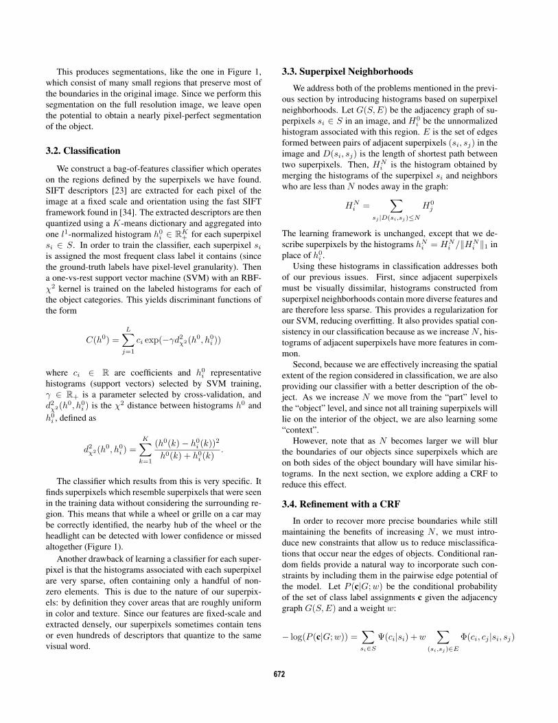
This produces segmentations, like the one in Figure 1,

which consist of many small regions that preserve most of

the boundaries in the original image. Since we perform this

segmentation on the full resolution image, we leave open

the potential to obtain a nearly pixel-perfect segmentation

of the object.

3.2. Classification

We construct a bag-of-features classifier which operates

on the regions defined by the superpixels we have found.

SIFT descriptors [23] are extracted for each pixel of the

image at a fixed scale and orientation using the fast SIFT

framework found in [34]. The extracted descriptors are then

quantized using a K-means dictionary and aggregated into

one l1-normalized histogram h0i ∈ R

K+ for each superpixel

si ∈ S. In order to train the classifier, each superpixel si

is assigned the most frequent class label it contains (since

the ground-truth labels have pixel-level granularity). Then

a one-vs-rest support vector machine (SVM) with an RBF-

χ2 kernel is trained on the labeled histograms for each of

the object categories. This yields discriminant functions of

the form

C(h0) =L∑

j=1

ci exp(−γd2χ2(h0, h0

i ))

where ci ∈ R are coefficients and h0i representative

histograms (support vectors) selected by SVM training,

γ ∈ R+ is a parameter selected by cross-validation, and

d2χ2(h0, h0

i ) is the χ2 distance between histograms h0 and

h0i , defined as

d2χ2(h0, h0

i ) =K∑

k=1

(h0(k)− h0i (k))2

h0(k) + h0i (k)

.

The classifier which results from this is very specific. It

finds superpixels which resemble superpixels that were seen

in the training data without considering the surrounding re-

gion. This means that while a wheel or grille on a car may

be correctly identified, the nearby hub of the wheel or the

headlight can be detected with lower confidence or missed

altogether (Figure 1).

Another drawback of learning a classifier for each super-

pixel is that the histograms associated with each superpixel

are very sparse, often containing only a handful of non-

zero elements. This is due to the nature of our superpix-

els: by definition they cover areas that are roughly uniform

in color and texture. Since our features are fixed-scale and

extracted densely, our superpixels sometimes contain tens

or even hundreds of descriptors that quantize to the same

visual word.

3.3. Superpixel Neighborhoods

We address both of the problems mentioned in the previ-

ous section by introducing histograms based on superpixel

neighborhoods. Let G(S, E) be the adjacency graph of su-

perpixels si ∈ S in an image, and H0i be the unnormalized

histogram associated with this region. E is the set of edges

formed between pairs of adjacent superpixels (si, sj) in the

image and D(si, sj) is the length of shortest path between

two superpixels. Then, HNi is the histogram obtained by

merging the histograms of the superpixel si and neighbors

who are less than N nodes away in the graph:

HNi =

∑sj |D(si,sj)≤N

H0j

The learning framework is unchanged, except that we de-

scribe superpixels by the histograms hNi = HN

i /‖HNi ‖1 in

place of h0i .

Using these histograms in classification addresses both

of our previous issues. First, since adjacent superpixels

must be visually dissimilar, histograms constructed from

superpixel neighborhoods contain more diverse features and

are therefore less sparse. This provides a regularization for

our SVM, reducing overfitting. It also provides spatial con-

sistency in our classification because as we increase N , his-

tograms of adjacent superpixels have more features in com-

mon.

Second, because we are effectively increasing the spatial

extent of the region considered in classification, we are also

providing our classifier with a better description of the ob-

ject. As we increase N we move from the “part” level to

the “object” level, and since not all training superpixels will

lie on the interior of the object, we are also learning some

“context”.

However, note that as N becomes larger we will blur

the boundaries of our objects since superpixels which are

on both sides of the object boundary will have similar his-

tograms. In the next section, we explore adding a CRF to

reduce this effect.

3.4. Refinement with a CRF

In order to recover more precise boundaries while still

maintaining the benefits of increasing N , we must intro-

duce new constraints that allow us to reduce misclassifica-

tions that occur near the edges of objects. Conditional ran-

dom fields provide a natural way to incorporate such con-

straints by including them in the pairwise edge potential of

the model. Let P (c|G;w) be the conditional probability

of the set of class label assignments c given the adjacency

graph G(S, E) and a weight w:

− log(P (c|G;w)) =∑si∈S

Ψ(ci|si) + w∑

(si,sj)∈E

Φ(ci, cj |si, sj)

672

Our unary potentials Ψ are defined directly by the proba-

bility outputs provided by our SVM [7] for each superpixel:

Ψ(ci|si) = − log(P (ci|si))

and our pairwise edge potentials Φ are similar to those of

[32, 6]:

Φ(ci, cj |si, sj) =(

L(si, sj)1 + ‖si − sj‖

)[ci �= cj ]

where [·] is the zero-one indicator function and ‖si − sj‖ is

the norm of the color difference between superpixels in the

LUV colorspace. L(si, sj) is the shared boundary length

between superpixels si and sj and acts here as a regulariz-

ing term which discourages small isolated regions.

In many CRF applications for this domain, the unary and

pairwise potentials are represented by a weighted summa-

tion of many simple features (e.g. [32]), and so the param-

eters of the model are learned by maximizing their condi-

tional log-likelihood. In our formulation, we simply have

one weight w which represents the tradeoff between spatial

regularization and our confidence in the classification. We

estimate w by cross validation on the training data. Once

our model has been learned, we carry out inference with the

multi-label graph optimization library of [4, 18, 5] using

α-expansion. Since the CRF is defined on the superpixel

graph, inference is very efficient, taking less than half a sec-

ond per image.

Results with the CRF are presented in Section 4 as well

as Figures 2 and 3.

4. Experiments

We evaluate our algorithm for varying N with and with-

out a CRF on two challenging datasets. Graz-02 contains

three categories (bicycles, cars and people) and a back-

ground class. The task is to localize each category against

the background class. Performance on this dataset is mea-

sured by the pixel precision-recall.

The PASCAL VOC 2007 Segmentation Challenge [9]

contains 21 categories and few training examples. While

the challenge specifies that the detection challenge training

data may also be used, we use only the ground truth seg-

mentation data for training. The performance measure for

this dataset is the average pixel accuracy: for each category

the number of correctly classified pixels is divided by the

ground truth pixels plus the number of incorrectly classi-

fied pixels. We also report the total percentage of pixels

correctly classified.

MATLAB code to reproduce our experiments is avail-

able from our website1.

1http://vision.ucla.edu/bag/

4.1. Common Parameters

Experiments on both datasets share many of the same

parameters which we detail here.

SIFT descriptors are extracted at each pixel with a patch

size of 12 pixels and fixed orientation. These descriptors are

quantized into a K-means dictionary learned on the training

data. All experiments we present here use K = 400, though

in Figure 1 we show that a wide variety of K produce simi-

lar results.

The superpixels extracted via quick shift are controlled

by three parameters: λ, the trade-off between color impor-

tance and spatial importance, σ, the scale at which the den-

sity is estimated, and τ , the maximum distance in the fea-

ture space between members of the same region. We use

the same parameters for all of our experiments: σ = 2, λ =0.5, τ = 8. These values were determined by segmenting a

few training images from Graz-02 by hand until we found a

set which preserved nearly all of the object boundaries and

had the largest possible average segment size. In principle,

we could do this search automatically on the training data,

looking for the parameter set which creates the largest aver-

age segment size while ensuring that the maximum possible

classification accuracy is greater than some desired level. In

practice, the algorithm is not too sensitive to the choice of

parameters, so a quick tuning by hand is sufficient. Note

that the number or size of the superpixels is not fixed (as op-

posed to [13]): the selected parameters put a rough bound

on the maximum size of the superpixels but do not con-

trol the shape of the superpixels or degree of the superpixel

graph.

Histograms for varying N are extracted as described in

Section 3.3 and labels are assigned to training superpixels

by the majority class vote. We randomly select an equal

number of training histograms from each category as the

training data for our SVM.

We learn a one-vs-rest multi-class SVM with an RBF-

χ2 kernel on the histograms using libsvm [7] as described

in Section 3.2. During testing, we convert our superpixel la-

bels into a pixel-labeled map and evaluate at the pixel level

for direct comparison with other methods.

In both experiments, we take our final SVM and include

it in the CRF model described in Section 3.4.

4.2. Graz-02

On Graz-02, we use the same training and testing split as

Marszałek and Schmid [24] and Fulkerson et al. [11]. Our

segment classifier is trained on 750 segments collected at

random from the category and the background.

Graz-02 images are 640 by 480 pixels and quick shift

produces approximately 2000 superpixels per image with

an average size of 150 pixels. The average degree of the su-

673

N=0

N=2 N=4

N=0

N=2 N=4

N=0

N=2 N=4

N=0

N=2 N=4

N=0

N=2 N=4

N=0

N=2 N=4

Figure 2. Graz-02 confidence maps. Our method produces very well localized segmentations of the target category on Graz-02. Here, a

dark red classification means that the classifier is extremely confident the region is foreground (using the probability output of libsvm), while

a dark blue classification indicates confident background classification. Notice that as we increase the number of neighbors considered (N )

regions which were uncertain become more confident and spurious detections are suppressed. Top two rows: Without CRF. Bottom tworows: With CRF.

Graz-02 N = PASCAL 2007 N =0 1 2 3 4 0 1 2 3 4

K = 10 37 44 47 51 49 10 10 12 12 12

K = 100 48 61 64 64 64 13 19 23 25 25

K = 200 49 63 66 66 64 13 20 25 26 25

K = 400 50 64 67 69 67 14 21 25 28 27

K = 1000 49 63 68 68 66 14 22 27 27 26

Table 1. Effect of K. Here we explore the effect of the dictionary

size K on the accuracy of our method (without a CRF) for vary-

ing neighborhood sizes N . Increasing the size of the dictionary

increases performance until we begin to overfit the data. We pick

K = 400 for our experiments, but a large range of K will work

well. Notice that even with K = 10 we capture some information,

and increasing N still provides noticeable improvement.

perpixel graph is 6, however the maximum degree is much

larger (137).

In Table 2, we compare our results for varying size Nwith those of Fulkerson et al. [11] which uses a similar

bag-of-features framework and Marszałek and Schmid [24]

which warps shape masks around likely features to define

probable regions. We improve upon the state-of-the-art in

all categories (+17% on cars, +15% on people, and +6% on

bicycles).

Example localizations may be found in Figures 1 and 2.

Cars People Bicycles

[24] full framework 53.8% 44.1% 61.8%

[11] NN 54.7% 47.1% 66.4%

[11] SVM 49.4% 51.4% 65.2%

N = 0 43.3% 51.3% 56.7%

CRF N = 0 46.0% 54.3% 63.4%

N = 1 62.0% 62.7% 67.6%

CRF N = 1 69.7% 63.8% 69.7%

N = 2 67.1% 65.4% 69.3%

CRF N = 2 71.2% 66.3% 71.2%

N = 3 68.6% 65.7% 71.7%

CRF N = 3 72.2% 66.1% 72.2%N = 4 67.1% 62.7% 71.0%

CRF N = 4 71.3% 63.2% 71.3%

Table 2. Graz-02 results. The precision = recall points for our

experiments on Graz-02. Compared to the former state-of-the-art

[11], we show a 17% improvement on Cars, a 15% improvement

on People and a 6% improvement on Bicycles. N is the distance of

the furthest neighboring region to aggregate, as described in Sec-

tion 3.3. Our best performing case is always the CRF-augmented

model described in Section 3.4.

Notice that although N = 0 produces some very precisely

defined correct classifications, there are also many missed

674

detections and false positives. As we increase the amount of

local information that is considered for each classification,

regions that were classified with lower confidence become

more confident, and false positives are suppressed.

Adding the CRF provides consistent improvement,

sharpening the boundaries of objects and providing further

spatial regularization. Our best performing cases use N = 2or N = 3, balancing the incorporation of extra local sup-

port with the preference for compact regions with regular

boundaries.

4.3. VOC 2007 Segmentation

For the VOC challenge, we use the same sized dictionary

and features as Graz-02 (K = 400, patch size = 12 pixels).

The training and testing split is defined in the challenge. We

train on the training and validation sets and test on the test

set. Since there are fewer training images per category, for

this experiment we train on 250 randomly selected training

histograms from each category.

VOC 2007 images are not fixed size and tend to be

smaller than those in Graz-02, so with the same parame-

ters quick shift produces approximately 1200 superpixels

per image with a mean size of 150 pixels. The average de-

gree of the superpixel graph is 6.4, and the maximum degree

is 72.

In Table 3 we compare with the only segmentation entry

in the challenge (Oxford Brookes), as well as the results of

Shotton et al. [31], and Pantofaru et al. [27]. Note that Shot-

ton reports a set of results which bootstrap a detection entry

(TKK). We do not compare with these results because we do

not have the data to do so. However, because our classifier

is simply a multi-class SVM, we can easily add either the

Image Level Prior (ILP) or a Detection Level Prior (DLP)

that Shotton uses. Even without the ILP, we find that we

outperform Shotton with the ILP on 14 of the 21 categories

and tie on one more. Our average performance is also im-

proved by 8%. Compared to Shotton without ILP or Panto-

faru, average performance is improved by 12%. Selected

segmentations may be found in Figure 3.

This dataset is much more challenging (we are separat-

ing 21 categories instead of 2, with less training data and

more variability) and because of this when N = 0 every-

thing has very low confidence. As we increase N we start

to see contextual relationships playing a role. For exam-

ple, in the upper left image of Figure 4 we see that as the

person classification gets more confident, so does the bike

and motorbike classification, since this configuration (per-

son above bike) occurs often in the training data. We also

see that larger N tends to favor more contiguous regions,

which is consistent with what we expect to observe.

On this dataset, adding a CRF improves the qualitative

results significantly, and provides a consistent boost for the

accuracy as well. Object boundaries become crisp, and of-

ten the whole object has the same label, even if it is not

always the correct one.

5. ConclusionWe have demonstrated a method for localizing objects

and segmenting object classes that considers the image at

the level of superpixels. Our method exceeds the state-of-

the-art on Graz-02 and the PASCAL VOC 2007 Segmen-

tation Challenge, even without the aid of a CRF or color

information. When we add a CRF which penalizes pairs of

superpixels that are very different in color, we consistently

improve both our quantitative and especially our qualitative

results.

Acknowledgments

This research was supported by ONR 67F-1080868/N0014-

08-1-0414 and NSF 0622245.

References[1] E. Aldea, J. Atif, and I. Bloch. Image classification using

marginalized kernels for graphs. In Proc. CVPR, 2007.

[2] K. Barnard, P. Duygulu, R. Guru, P. Gabbur, and D. Forsyth.

The effects of segmentation and feature choice in a transla-

tion model of object recognition. In Proc. CVPR, 2003.

[3] M. Blaschko and C. Lampert. Learning to localize objects

with structured output regression. In Proc. ECCV, 2008.

[4] Y. Boykov and V. Kolmogorov. An experimental comparison

of min-cut/max-flow algorithms for energy minimization in

vision. In PAMI, 2004.

[5] Y. Boykov, O. Veksler, and R. Zabih. Efficient approximate

energy minimization via graph cuts. In PAMI, 2001.

[6] Y. Y. Boykov and M.-P. Jolly. Interactive graph cuts for op-

timality boundary & region segmentation of objects in N-D

images. In Proc. ICCV, 2001.

[7] C.-C. Chang and C.-J. Lin. LIBSVM: a library for sup-port vector machines, 2001. Software available at http://www.csie.ntu.edu.tw/˜cjlin/libsvm.

[8] N. Dalal and B. Triggs. Histograms of oriented gradients for

human detection. In Proc. CVPR, 2005.

[9] M. Everingham, L. Van Gool, C. K. I. Williams, J. Winn,

and A. Zisserman. The PASCAL Visual Object Classes

Challenge 2007 (VOC2007) Results. http://www.pascal-

network.org/challenges/VOC/voc2007/workshop/index.html.

[10] P. F. Felzenszwalb and D. P. Huttenlocher. Efficient graph-

based image segmentation. IJCV, 59(2), 2004.

[11] B. Fulkerson, A. Vedaldi, and S. Soatto. Localizing objects

with smart dictionaries. In Proc. ECCV, 2008.

[12] C. Galleguillos, B. Babenko, A. Rabinovich, and S. Be-

longie. Weakly supervised object localization with stable

segmentations. In Proc. ECCV, 2008.

[13] S. Gould, J. Rodgers, D. Cohen, G. Elidan, and D. Koller.

Multi-class segmentation with relative location prior. In

IJCV, 2008.

675

N=0

N=2 N=4

N=0

N=2 N=4

N=0

N=2 N=4

N=0

N=2 N=4

N=0

N=2 N=4

N=0

N=2 N=4

N=0

N=2 N=4

N=0

N=2 N=4

N=0

N=2 N=4

N=0

N=2 N=4

N=0

N=2 N=4

N=0

N=2 N=4

Figure 3. PASCAL VOC 2007 + CRF. Some selected segmentations for PASCAL. For each test image, the results are arranged into two

blocks of four images. The first block (left-to-right) shows the results of the superpixel neighborhoods without a CRF. The second block

uses the CRF described in Section 3.4. Colors indicate category and the intensity of the color is proportional to the posterior probability of

the classification. Best viewed in color.

bac

kg

rou

nd

aero

pla

ne

bic

ycl

e

bir

d

bo

at

bo

ttle

bu

s

car

cat

chai

r

cow

din

ing

tab

le

do

g

ho

rse

mo

torb

ike

per

son

po

tted

pla

nt

shee

p

sofa

trai

n

tvm

on

ito

r

Aver

age

%Pi

xels

Brookes 78 6 0 0 0 0 9 5 10 1 2 11 0 6 6 29 2 2 0 11 1 9 -

[27] 59 27 1 8 2 1 32 14 14 4 8 32 9 24 15 81 11 26 1 28 17 20 -

[31] 33 46 5 14 11 14 34 8 6 3 10 39 40 28 23 32 19 19 8 24 9 20 -

[31] + ILP 20 66 6 15 6 15 32 19 7 7 13 44 31 44 27 39 35 12 7 39 23 24 -

N = 0 21 14 8 8 17 14 10 7 19 13 13 7 16 9 13 2 10 23 34 17 20 14 18

CRF+N = 0 20 14 8 8 17 14 10 7 19 13 13 7 16 9 13 2 10 23 34 17 20 14 18

N = 1 27 27 20 17 14 12 18 11 37 18 7 14 26 19 35 18 13 21 25 31 25 21 25

CRF+N = 1 38 32 20 13 17 10 20 11 52 17 7 14 31 21 39 28 14 12 28 42 33 24 34

N = 2 36 27 26 15 11 5 26 29 42 25 9 15 36 23 58 32 17 11 20 37 29 25 34

CRF+N = 2 56 26 29 19 16 3 42 44 56 23 6 11 62 16 68 46 16 10 21 52 40 32 51

N = 3 47 22 24 17 11 6 35 25 46 19 8 19 33 29 62 47 16 20 26 37 29 28 43

CRF+N = 3 65 22 28 32 2 4 40 30 61 10 3 20 35 24 72 62 16 23 20 44 30 30 57N = 4 51 20 22 18 7 2 39 25 49 15 6 14 36 28 64 56 15 17 21 40 23 27 46

CRF+N = 4 65 20 30 22 2 2 39 25 57 10 3 7 36 23 66 62 15 17 8 46 11 27 57

Table 3. VOC 2007 segmentation results. Our best overall average performance (CRF+N = 2) performs better than Shotton et al. [31]

with or without an Image Level Prior (ILP) on 14 out of 21 categories. Note that we could add ILP to our model. Similarly, we do not

compare with the Shotton et al. results which used TKK’s detection results as a Detection Level Prior (DLP) because TKK’s detections

were not available. We expect our method would provide a similar performance boost with this information. The CRF provides consistent

improvment in average accuracy and in the percentage of pixels which were correctly classified.

676

bicycle N=0

N=2 N=4

N=0

N=2 N=4

diningtable N=0

N=2 N=4

N=0

N=2 N=4

horse N=0

N=2 N=4

N=0

N=2 N=4

aeroplane N=0

N=2 N=4

N=0

N=2 N=4

Figure 4. PASCAL VOC 2007 Confidence. Confidence maps for PASCAL. The results are arranged into two blocks of four images for

each test image. The first block contains the input image, a category label, and the confidence map for that category for N = 0, 2, 4. The

second block contains the ground truth labeling and our labellings with an intensity proportional to the confidence of the classification.

Colors indicate category. For example, in the upper left we show the confidence for bicycle, and the classification which contains mostly

bicycle (green) and some motorbike (light blue).

[14] Z. Harchaoui and F. Bach. Image classification with segmen-

tation graph kernels. In Proc. CVPR, 2007.

[15] X. He, R. Zemel, and M. C.-P. nan. Multiscale conditional

random fields for image labeling. In Proc. CVPR, 2004.

[16] X. He, R. Zemel, and D. Ray. Learning and incorporating

top-down cues in image segmentation. In Proc. ECCV, 2006.

[17] D. Hoiem, C. Rother, and J. Winn. 3d layoutcrf for multi-

view object class recognition and segmentation. In Proc.CVPR, 2007.

[18] V. Kolmogorov and R. Zabih. What energy functions can be

minimized via graph cuts? In PAMI, 2004.

[19] S. Kumar and M. Hebert. A hierachical field framework for

unified context-based classification. In Proc. ICCV, 2005.

[20] J. Lafferty, A. McCallum, and F. Pereira. Conditional ran-

dom fields: Probabilistic models for segmenting and labeling

sequence data. In Proc. ICML, 2001.

[21] C. Lampert, M. Blaschko, and T. Hofmann. Beyond sliding

windows: Object localization by efficient subwindow search.

In Proc. CVPR, 2008.

[22] S. Lazebnik, C. Schmid, and J. Ponce. Beyond bag of

features: Spatial pyramid matching for recognizing natural

scene categories. In Proc. CVPR, 2006.

[23] D. G. Lowe. Distinctive image features from scale-invariant

keypoints. IJCV, 2(60):91–110, 2004.

[24] M. Marszałek and C. Schmid. Accurate object localization

with shape masks. In Proc. CVPR, 2007.

[25] A. Moore, S. Prince, J. Warrell, U. Mohammed, and

G. Jones. Superpixel lattices. In Proc. CVPR, 2008.

[26] S. Nowozin, K. Tsuda, T. Uno, T. Kudo, and G. BakIr.

Weighted substructure mining for image analysis. In Proc.CVPR, 2007.

[27] C. Pantofaru, C. Schmid, and M. Hebert. Object recogni-

tion by integrating multiple image segmentations. In Proc.ECCV, 2008.

[28] A. Rabinovich, A. Vedaldi, C. Galleguillos, E. Wiewiora,

and S. Belongie. Objects in context. In Proc. ICCV, 2007.

[29] X. Ren and J. Malik. Learning a classification model for

segmentation. In Proc. ICCV, 2003.

[30] B. C. Russell, A. A. Efros, J. Sivic, W. T. Freeman, and

A. Zisserman. Using multiple segmentations to discover ob-

jects and their extent in image collections. In Proc. CVPR,

2006.

[31] J. Shotton, M. Johnson, and R. Cipolla. Semantic texton

forests for image categorization and segmentation. In Proc.CVPR, 2008.

[32] J. Shotton, J. Winn, C. Rother, and A. Criminisi. Texton-Boost: Joint appearance, shape and context modeling for

multi-class object recognition and segmentation. In Proc.ECCV, 2006.

[33] S. Soatto. Actionable information in vision. In Proc. ICCV,

October 2009.

[34] A. Vedaldi and B. Fulkerson. VLFeat: An open and portable

library of computer vision algorithms. http://www.vlfeat.org/, 2008.

[35] A. Vedaldi, V. Gulshan, M. Varma, and A. Zisserman. Mul-

tiple kernels for object detection. In Proc. ICCV, 2009.

[36] A. Vedaldi and S. Soatto. Quick shift and kernel methods for

mode seeking. In Proc. ECCV, 2008.

[37] J. Verbeek and B. Triggs. Region classification with markov

field aspect models. In Proc. CVPR, 2007.

677