Class and Channel Condition Based Weighted Proportional FairScheduler

Rajeev Agrawala , Anand Bedekara, Richard J. Laa, and Vijay Subramaniana

a Mathematics of Communication NetworksMotorola Inc., Arlington Heights, IL, USA 60004.

In this paper we outline a scheme to perform packet-level scheduling and resourceallocation at the wireless node that takes into account the notions of both efficiency andfairness and presents a means to explore the trade-off between these two notions. Asa part of this scheme we see the scheduling problem as deciding not just the packettransmission schedule but also the power allocation, the modulation and coding schemeallocation and the spreading code determination since the latter three directly influencethe radio resources consumed. Using a utility maximization formulation based on thedata-rates that the mobiles can transmit at, we decide on the weights for a weightedproportionally fair allocation based scheduling algorithm. We conclude with a simulationbased performance analysis for infinitely-backlogged sources on a UMTS system.

1. INTRODUCTION

The explosion of multimedia services on the Internet is leading to a demand of the sameservices in the non-tethered wireless space. There are, however, many peculiarities thata wireless channel possesses which makes supporting such services much tougher thanon wireline networks. One of the key elements in this is the scheduler used at variousnodes. Scheduling in traditional wireline networks consists mainly of deciding the order inwhich users access the channel. This is because it is quite easy to use these channels veryclose to their (information theoretic) capacity at any given power (used on the channel).Thus, it is best to operate at the maximum capacity by using the maximum power allthe time. In addition, the channels, and thus the data rates, are not time-varying either.On wireless channels, however, there are many considerations which do not allow for sucha mode of operation. The bandwidth available for transmission on a wireless channeland the power levels allowed (both regulated) put a hard limit on the capacity1. Anotherimportant element is the mobility of the end-user equipment which results in time-varyingmultipath and fading. Further, the size, battery power, and processing power of the enddevices place additional constraints on system performance. Limited battery capacity alsomakes it necessary to use transmission schemes that would prolong battery life as much aspossible. Finally, the multiuser nature of a wireless channel makes it interference-limited.Thus, one user transmitting at maximum power could severely impair the transmissions

1The propagation characteristics of the atmosphere, and other media, are also deciding factors for theband of operation and hence, the bandwidth.

of other users. Thus, using a traditional wireline scheduler is not a good approach on awireless channel.

Some of recent developments in wireless link scheduling include the work by Holtzman[1], Jalali et al. [2], Tse [3], Shakkottai and Stolyar [4], Chawla et al. [5], Leelahakriengkrai[6], and Berry and Gallager [7]. All of these works show that substantial benefits areachieved when the higher layers are aware of the radio conditions and can adapt thepowers, the modulation schemes, the coding schemes, and spreading gains (and hence thedata rates) based upon this knowledge. The upshot of this is that scheduling policiesshould be devised using the knowledge of channel conditions. In a cellular context thereis an additional benefit to the network layer control of transmission strategies. In sucha situation it is possible to trade capacity among cells (by changing the power levels, forinstance) to alleviate periods of congestion or high demand. From the discussion above itis clear that a scheduler that jointly performs packet-level scheduling and radio-resourceallocation is the solution for the wireless-link scheduling problem. To be able to implementsuch scheduling policies it is necessary to have a system that has controls in place to allowfor changing the transmission parameters easily. The third-generation (3G) technologiesare a first step in this direction. Nanda et al. [8] provide a fairly comprehensive overviewof the 3G technologies and how they have been designed with multimedia-type servicesin mind. In all proposals it is possible for connections to not only choose from a varietyof data rates but also change the data rate in a flexible and quick fashion. There isalso added feedback, in terms of more frequent error and measurement reports, which inconjunction with flexible data rate allocation, can in turn be used for a better monitoringof QoS guarantees and provisioning of resources.

Since the radio resource is quite expensive the efficient management of this resource iscritical. This, however, cannot be the only concern when QoS parameters have been agreedto for various users and when the operator is obliged to uphold them. Thus, it is imperativeto have some fairness in the arbitration of resources amongst the various users. In thispaper we outline a scheme to perform packet-level scheduling and resource allocationat the wireless (access) node that takes into account the notions of both efficiency andfairness and presents a means to explore the trade-off between these two notions. Thistrade-off between efficiency and fairness was not a concern of earlier cellular systemsbecause voice was the major application and thus, only coverage (which is in realityjust another terminology for fairness) was critical. It is only with the emergence of the3G technologies and packetized data services that such a trade-off makes any sense. Inwireline networking there are two broad philosophies when QoS provisioning is considered.One follows the IntServ approach and attempts to provide strict QoS guarantees [9].Another approach uses the ideas in DiffServ to provide a class-based differentiation ofservices [10]. Differentiated services are supported through various per-hop-behaviors(PHBs) in DiffServ capable networks. For instance, expedited forwarding (EF) is aimedat supporting real-time applications such as video conferencing. Other PHBs, such asassured forwarding (AF) [11] and best effort (BE), support non-real-time applicationsthat do not require strict delay guarantees. AF can further have different services, forinstance, Gold, Silver, and Bronze services.

The work in [4,6] is more in the IntServ context and they schedule users based upon theircurrent backlog to satisfy statistical delay guarantees. With such scheduling mechanisms

one needs a good admission control policy and policing mechanism in place. The work inthis paper is based on the DiffServ philosophy where we provide a differentiation basedupon both class and channel-state. Further, we restrict our attention to non-real-time(rate-adaptive) services. The reason we choose to provide a service differentiation basedupon channel-state is because this determines how much network resource is utilized bythe application. This is very much in keeping with similar differentiation in wirelinenetworks with protocols like TCP using quantities like round-trip time estimates andhop-count as surrogates for measuring how much of the network resource is utilized byvarious applications. The work in [1–3,5] also adheres to the DiffServ philosophy. Inthe proposed algorithm in this paper we suggest a flexible way of trading off efficiencyfor fairness as well as a flexible means of exploiting temporary fluctuations in channelconditions.

In Section 2 we give a detailed introduction to the wireless link scheduling problem.Thereafter, we introduce a related resource allocation problem in Section 3 and presentour scheduling algorithm in Section 4. A performance analysis of the algorithm withinfinitely-backlogged sources is discussed in Section 5. Finally, we conclude in Section 6.

2. THE WIRELESS LINK SCHEDULING PROBLEM

Consider a cellular system. In a given cell b let Jb be the set of users on the downlink.Time is slotted into radio blocks (in GPRS and EDGE) or frames in (cdma2000 andUMTS) of fixed duration (20, 10, or 3.33 ms depending on the technology). We shall referto these time slots as frames hereafter. The wireless link scheduling problem is one ofdeciding which of these users transmit in each frame. In a TDMA system like GPRS andEDGE only one user is allowed to transmit in a frame, whereas in a CDMA system likecdma2000 or UMTS multiple users may transmit in a frame. When a user transmits, wealso need to decide what power level, modulation and coding scheme, time slot (in caseof TDMA) and spreading factor (in case of CDMA) it will use.

Due to different base site to user distances, shadow fading and multipath, the channelconditions of different users vary with time. This fluctuation in channel conditions resultsin a variation of the effective data rate (per channel per unit power) R̂j(t) available tothe different users j ∈ Jb in different frames t = 0, 1, . . .. This effective data rate perunit resource may be calculated in a variety of ways. We outline two simple ones below.Consider the signal to interference plus noise ration (SINR) of user j

SINRj(t) =Pj(t)Gjj(t)∑

i6=j Pi(t)Gij(t) + σ2, (1)

where Pj(t) is the transmit power of user j, σ2 is the receiver noise variance and Gij(t) isthe energy gain from base station of mobile station i to mobile station j. Once SINRj(t)’sare available for the users (either using the above formula or direct measurements), onecan compute the data rates and frame error rates (FER) corresponding to different choicesof modulation and coding schemes (MCSs) and/or spreading factors (SFs). Hence, onecan find the choice of MCS and/or SF that maximizes Rj(1−FER), where Rj and FERare the data rate and frame error rate of user j corresponding to the MCS and/or SF,respectively.

In case of a TDMA system where we do not share the transmit power of the base stationacross multiple users in the same frame, we may consider the transmit power fixed. Inthis case the resulting optimum above may be considered to be the effective data rate perunit resource R̂j(t).

In a CDMA system we may consider the energy per bit to noise power-spectral-densityratio (Eb/N0) given by:(EbN0

)j

(t) =W

Rj(t)SINRj(t) =

W

Rj(t)

Pj(t)Gjj(t)∑i6=j Pi(t)Gij(t) + σ2

(2)

where W is the channel bandwidth and W/Rj is user j’s spreading factor. As a surrogateto controlling the FER we may attempt to satisfy an Eb/N0 target Γj. Let the smallestbit rate allowed (corresponding to the largest SF) be Rmin. We may think of this as aCDMA channel. Then we can define the effective data rate per channel per unit power as

R̂j(t) =Rj(t)/Rmin

Pj(t)=

W

RminΓj

Gjj(t)∑i6=j Pi(t)Gij(t) + σ2

(3)

What follows does not depend on precisely how R̂j(t) is defined and measured. Thekey idea is that it will be monotonically increasing in the users’ own channel gain anddecreasing in interference plus noise.

Let Mb channels be available and let Pb be the power available per channel at base siteb. In each frame t we have to decide what fraction ρj(t) > 0 of the resources (channelsand powers) will be allocated to the different users j ∈ Jb;

∑j∈Jb ρj(t) ≤ 1. In which case

it gets a throughput rj(t) = R̂j(t)ρj(t)PbMb (if all of the channel and power resources are

given to user j, then it would get a throughput rj = R̂j(t)PbMb). Typically there will beadditional constraints on ρj(t) depending on the technology as described below.

In a TDMA system, like GPRS or EDGE, Mb denotes the number of time slot channelsavailable (Mb = 1, . . . , 8). One and only one user can transmit in a time slot in a frame,so ρj(t)Mb must be an integer. Additional restrictions on allocation of time slots to usersmay further constrain ρj(t).

In a CDMA system like cdma2000 or UMTS, Mb may be the number of spreading codes(a code representing the smallest data rate allocation Rmin) available and Pb be the powerper code available, in which case MbPb is the total power budget at base site b. Let fj(t)be the fraction of spreading codes given to user j and let pj(t) be the fraction of per codepower to be used by user j. Then fj(t)Mb will be the number of codes given to user j andmust be an integer (it may even have to be a power of 2). pj(t) may be an arbitrary realnumber; pj(t)Pb will be the power per code and fj(t)Mbpj(t)Pb the total power given touser j. We may require that the power per code given to user j be such that it satisfiesa certain Eb/N0 target (2). Of course we will need that

∑j∈Jb fj(t)Mbpj(t)Pb ≤ MbPb or

that∑j∈Jb ρj(t) ≤ 1, where ρj(t) = fj(t)pj(t).

In summary, the wireless link scheduling problem requires that in each frame t wedecide what fraction ρj(t) ≥ 0 of the resources (channels and powers) will be allocatedto the different users j ∈ Jb;

∑j∈Jb ρj(t) ≤ 1, in which case it gets a throughput rj(t) =

R̂j(t)ρj(t)PbMb. Since R̂j(t) varies with both the user and time we would like to dothe scheduling in such a way that we capitalize on these variations to get high systemthroughput while providing some level of QoS differentiation.

3. BASIC ALGORITHM

In the previous section we have considered the resource allocation problem on a frame-by-frame basis. This requires that the number of resources allocated to the users need bean integer. However, in the following sections as a first step of designing the schedulingalgorithm we relax this constraint and consider the framework where we are interestedin finding the fraction of resources to be allocated to the users over a sufficiently largeperiod.

Given the effective data rate per unit resource R̂j of the users as described in Sec-tion 2 we compute the fraction of the resources that will be allocated to each user j fortransmission by solving the following optimization problem:

maxρj

∑j∈Jb

Uj(ρjR̂jPbMb) (4)

subject to∑j∈Jb

ρj ≤ 1

ρj ≥ 0,

where Uj(·) is the utility function of user j as a function of the throughput it receives. Theoptimization problem in (4) computes the solution that maximizes the aggregate utilityof the users given the resource and non-negativity constraints.

We first characterize the solution of (4) with the most commonly used utility functionsof

Ui(ri) = fα(ri) =

{sgn(α) · rαi , if α 6= 0, α < 1log(ri), if α = 0.

(5)

With the utility functions of fα(·), one can show that the solution of the optimizationproblem in (4) is given by

ρj =(R̂j)

β−1∑k∈Jb(R̂k)β−1

∝ (R̂j)β−1, (6)

where β = 11−α . Note that if α is greater than zero, the allocation favors users with higher

R̂j, and if α is less than zero, the allocation favors users with lower R̂j. The value of αequal to one leads to efficiency only solution in that all slots are allocated to the userswith the highest R̂j, while a value of α close to −∞ yields a fairness only solution in thatevery user receives approximately the same rate. In this sense the parameter α controlsthe extent to which this bias is enforced and hence how efficiency, i.e., throughput, istraded off in favor of fairness.

After computing the solution ρ∗ to (4) we compute the credits Cj for the users, where

the credit of user j is Cj = ρ∗j · R̂j. Note that the credit, Cj, of user j would be thethroughput of the user normalized by PbMb if it indeed received ρ∗j of the resources.However, due to various system constraints a user’ throughput may differ from its credit.For instance, in EDGE users are placed on one or more time slots, depending on whetherthey are single or multiple slot capable. A user’s actual rate depends both on its ρ∗jand time slot configuration. In a CDMA system users may have maximum data-rate

constraints or maximum power constraints. Incorporating these system constraints intothe optimization problem leads to a weighted proportionally fair2 (WPF) allocation [12,Eqn. (2)] with weights Cj

R̂jas proved in the following proposition.

Proposition 3.1 The weighted proportionally fair rates with the weights CjR̂j

s are also

the optimal solution to the problem in (4) with the addition of the system constraintsmentioned above.

Proof: See [13].

4. THE CLASS AND CHANNEL CONDITION BASED WEIGHTED PRO-PORTIONAL FAIR (C3WPF ) SCHEDULER

In our algorithm that is described in this section we use users’ credits to allocatethe available bandwidth. The idea behind the algorithm is to mimic the behavior ofweighted fair queueing (WFQ) without explicitly computing the virtual times for thearriving protocol data units (PDUs). The credits Cj are similar to the weights φj inWFQ. We show that our algorithm leads to a weighted proportionally fair (WPF) rateallocation in the sense that the users that have the same set of bottlenecks or systemconstraints receive rates that are proportional to their credits.

We first consider the simple case where the channel conditions and thus the effectivedata rates per unit resource of the users are time-invariant so as to explain the key ideabehind our algorithm. Then, we describe the actual algorithm that uses the values ofcurrent and average effective data rates per unit resource of the users.

4.1. A Simple Algorithm for Time-invariant ChannelsEach user has a traffic class associated with its connection. For instance, in EDGE

there are six traffic classes: conversational, streaming, interactive best-effort (I1, I2, andI3), and background best-effort. Associated with each traffic class is a weight w. Thisweight may reflect the price charged to the traffic class per unit time of usage [14,15] andis used in the computation of credits in order to provide differentiated services among thetraffic classes.

The scheduling algorithm described below attempts to deliver throughtputs propor-tional to credits Cj = wjR̂

βj , which reflects both users’ traffic classes and channel con-

ditions. However due to additional constraints on slots, powers, codes, etc., this preciseproportion may not be obtainable. We would therefore like to obtain the weighted pro-portional fair (WPF) solution with weights equal to the credits. In order to achieve thiswe use the following algorithm described below:

Let Wj(t) be the total throughput of user j up to time t. Let W̄j(t) := Wj(t)/Cjbe the throughput normalized by credits. At time t + 1 we sort users in increasingorder of their W̄j(t). The scheduler then picks the user at the front of this list andschedules it for transmission in frame t + 1. At the same time it determines the channeland power resources needed for this user. Should resources remain, it goes down the

2A vector of rates r∗ is said to be weighted proportionally fair with weights p if and only if it is feasibleand for any other feasible rate vector r it satisfies

∑j pj

rj−r∗jr∗j≤ 0.

sorted list, in order, to select additional users for transmission in that frame. Usersselected for transmission should obviously have data to send in that frame. Note thatby favoring users with low W̄ (t) for transmission, this algorithm tries to equalize thenormalized throughputs W̄j(t) over all users j ∈ Jb as time t→∞ so as to get throughputsproportional to their credits Cj. However as mentioned earlier this may not be feasible dueto additional constraints. The best achievable in that case would be the WPF throughputallocation in the sense that the users with the same system constraints would receive ratesproportional to their credits. We show below that this algorithm does deliver the WPFthroughputs asymptotically.

Proposition 4.1 The average throughputs of the users, i.e., Wj(t)

t, converge asymptoti-

cally to the weighted proportionally fair rates with the weights CjR̂j

s as t→∞.

Proof: See [13].From this we have the following corollary.

Corollary 4.1 The average throughputs of the users, i.e., Wj(t)

t, converge asymptotically

to the optimal rates as t→∞.

Note from the definition of the credits that two users with the same channel conditions(R̂js) can ask for different service based upon the weight of the class they subscribe to.

4.2. The Actual Algorithm for Time-varying ChannelsIn the algorithm described above we have assumed that the channel conditions, as

captured in the effective data rate per unit resource R̂j, do not vary with time. Wenow describe the actual algorithm that can take advantage of the time-varying channelconditions of the users to improve the system throughput. The key change is in thevalues of R̂j used above and in the update equation for W̄j. Let R̂j(t) be the current

effective data rate per unit resource based on current channel conditions. Let R̂avj (t) be

corresponding average obtained using geometric IIR filtering, i.e.,

R̂avj (t+ 1) = ψ · R̂av

j (t) + (1− ψ)R̂j(t) . (7)

The credits calculated use both R̂j(t) and R̂avj (t) as

Cj(t) = wj(R̂avj (t))β

R̂j(t)

R̂avj (t)

γ = wj(R̂avj (t))β−γ(R̂j(t))

γ = C1j (t)C2

j (t) , (8)

where 0 ≤ γ ≤ β. The value of γ should depend on how accurate or reliable R̂j(t)’sare. We use different factorizations of Cj(t) into C1

j (t) and C2j (t) to construct different

scheduling algorithms.Let Dj(t) be the amount of data transmitted in frame t for user j. W̄ is updated as

per the following algorithm.

W̄j(t+ 1) = φ · W̄j(t) + (1− φ)Dj(t)

C1j (t)

(9)

In keeping with the algorithm described earlier, at the beginning of time frame t+ 1, wesort users in increasing order of W̄j(t + 1)/C2

j (t) and select users for transmission basedon available resources.

Currently we have three different scheduling algorithms:

• Variant 1: For this we use C1j (t) = Cj(t) and C2

j (t) = 1.

• Variant 2: Here we use C1j (t) = wj(R̂

avj (t))β and C2

j (t) = ( R̂j(t)

R̂avj (t)

)γ.

• Variant 3: Here we use C2j (t) = Cj(t) and C1

j (t) = 1. Note that this resemblesthe algorithm analyzed earlier; the time-invariant credit value is substituted by atime-varying definition of credit.

Note that choosing the credits as described above does two things. Since the effectivedata rate per unit resource R̂j(t) is time varying, it uses an estimate R̂av

j (t) for its average.The estimate is based on an IIR filter; other estimates may easily be substituted. If weset γ = 0 above, then we will simply be biasing the throughput in proportion to thisaverage (raised to the power β). However, by dividing by non-unity values of the factorC2(j(t) (in variants 2 and 3), we tend to favor those users that have better channelconditions relative to their own average conditions. This second idea is also exploited inthe scheduling algorithms proposed by Holtzman [1], Tse [3], and Jalali et al. [2]. Infact the algorithm proposed is similar to Variant 3 proposed above with β = γ = 1. Onemajor difference is that they use a time-average computation of W̄ instead of the IIR filterestimator in (9). The time constant in the IIR filter estimator for the average must bechosen depending on how frequently channel condition measurements are available andthe time constants involved in the channel fluctuations (distance based path loss, shadowfading, and fast fading).

5. PERFORMANCE ANALYSIS

In this section we describe our experiments with the proposed scheduling algorithm.In addition to evaluating the performance of the algorithm in a simplistic setting, weare also interested in comparing the performance of a scheduling algorithm that is awareof the channel conditions with a scheduling approach that does packet-level schedulingseparate from radio-resource allocation. Henceforth in this document we refer to the classof schedulers that are not aware of channel conditions as split-schedulers. The specificsplit-scheduler that we consider is one that tries to equalize the data rates that all theusers get. Note that this can be easily achieved in the framework of our algorithm bysetting β = 0. This is equivalent to a WFQ scheduler with equal weights. Throughoutthe performance analysis section we concentrate on a UMTS system.

5.1. Simulation Set-upIn this sub-section we describe the set-up for our performance analysis. First we de-

scribe the physical constraints, and thereafter the network-level characteristics like trafficsources, fragmentation and ARQ-mechanisms.

We consider a system with 25 cells, which use the same carrier and the same sector,and 15 mobiles in each cell. The positions of the mobiles are chosen at random, spatially

Table 1Parameters used for UMTS simulation experiments.Number of data mobiles per cell 15Number of voice users per cell 32BTS max. transmit power 40 dBm = 10 WNon-orthogonality factor α 0.4Allowed bits / frame 2400, 1800, 1200, 600, 300Max. total bits / frame 14400 (3/4 of code tree)Power consumed by overhead channels 30% of BTS powerInter Base-site spacing 2800 mShadow Fading offSimulation time 25 sChip rate 3.84 McpsSystem bandwidth 5 MhzNoise Power 1.214× 10−10 mW = −99 dBmMobile speed 3 km/h

uniform in an annulus that extends half-way into the cell starting from the edge of the celland kept fixed for the entire simulation. The UMTS frames are 10 ms in duration. Sincethe system is a CDMA system we use a reuse factor of one and for simplicity also assumethat we have no sectorization. We model fast fading using the Jakes simulator [16] butdo not incorporate log-normal shadow fading terms in the propagation loss coefficients.Each cell has a power budget that cannot be exceeded. A part of this power budget isconsumed by control channels. After allocating power to the control channels we allocatenon-zero power values, such that their sum does not exceed the remaining power budget,to the voice users and then add the data users in one at a time using the W̄ ordering.In addition to a power-budget we also have a code-allocation check that checks to see ifa valid code is available. For all our simulation experiments we assume that there are32 voice users in the system. Open-loop power control on a fast time-scale (1500 Hz)is also implemented in the simulations. The parameters used for the experiments aresummarized in Table 1.

We assume that all the sources for our experiments are infinitely back-logged sources.We also assume that we get instantaneous feedback for the transmissions on the wirelesschannel and the erroneous frame is immediately put back at the head-of-the-line fortransmission. Thus, we are assuming that our ARQ mechanism transmits packets tillthey are correctly received. The ARQ mechanism also reacts instantaneously to bearer-type (data rate) changes recommended by the power-budget calculation and code-checkalgorithm fragmenting in a way such that it transmits the right number of bits in eachframe.

5.2. Simulation ExperimentsIn this set-up we try β = 0, 1, and 2, which would allow us to compare the split round-

robin scheduler (β = 0) with a scheduler that uses U(x) = log(x) (β = 1) as the utilityfunction and another that uses U(x) =

√x as the utility function (β = 2). We also seek

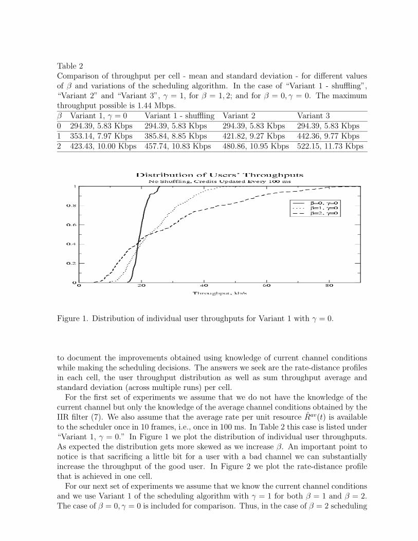
Table 2Comparison of throughput per cell - mean and standard deviation - for different valuesof β and variations of the scheduling algorithm. In the case of “Variant 1 - shuffling”,“Variant 2” and “Variant 3”, γ = 1, for β = 1, 2; and for β = 0, γ = 0. The maximumthroughput possible is 1.44 Mbps.β Variant 1, γ = 0 Variant 1 - shuffling Variant 2 Variant 30 294.39, 5.83 Kbps 294.39, 5.83 Kbps 294.39, 5.83 Kbps 294.39, 5.83 Kbps1 353.14, 7.97 Kbps 385.84, 8.85 Kbps 421.82, 9.27 Kbps 442.36, 9.77 Kbps2 423.43, 10.00 Kbps 457.74, 10.83 Kbps 480.86, 10.95 Kbps 522.15, 11.73 Kbps

Figure 1. Distribution of individual user throughputs for Variant 1 with γ = 0.

to document the improvements obtained using knowledge of current channel conditionswhile making the scheduling decisions. The answers we seek are the rate-distance profilesin each cell, the user throughput distribution as well as sum throughput average andstandard deviation (across multiple runs) per cell.

For the first set of experiments we assume that we do not have the knowledge of thecurrent channel but only the knowledge of the average channel conditions obtained by theIIR filter (7). We also assume that the average rate per unit resource R̂av(t) is availableto the scheduler once in 10 frames, i.e., once in 100 ms. In Table 2 this case is listed under“Variant 1, γ = 0.” In Figure 1 we plot the distribution of individual user throughputs.As expected the distribution gets more skewed as we increase β. An important point tonotice is that sacrificing a little bit for a user with a bad channel we can substantiallyincrease the throughput of the good user. In Figure 2 we plot the rate-distance profilethat is achieved in one cell.

For our next set of experiments we assume that we know the current channel conditionsand we use Variant 1 of the scheduling algorithm with γ = 1 for both β = 1 and β = 2.The case of β = 0, γ = 0 is included for comparison. Thus, in the case of β = 2 scheduling

Figure 2. Typical rate-distance profile for Variant 1 with γ = 0.

is based on both the current and average channel conditions whereas for β = 1 it is basedonly on the current conditions. In Table 2 this case is listed under “Variant 1- shuffling.”Figures 3 and 4 display the same quantities as in the earlier two figures respectively.

For our final set of experiments we consider Variant 3 of the scheduling algorithm withγ = 1 for β = 1, 2. Variant 3 with β = γ = 1 is similar to the algorithm proposed in[1,3,2]. An important difference is that the algorithm in [1,3,2] allows for only one userper frame. With maximum power constraints or maximum rate constraints this would bewasteful of power. They also concentrated on a CDMA2000 system with 3.33ms frames.In our simulation of their algorithm we allow for many users to be scheduled during eachframe and, in addition, use an IIR filter estimate of W̄ . This falls under the case of β = 1and γ = 1. In Table 2 this set of experiments is listed under “Variant 3.” Figures 5 and6 once again plot the same quantities as in Figures 1 and 2, respectively.

We see from Table 2 that the system throughputs increase dramatically with the knowl-edge of channel conditions. It is interesting to note that with the knowledge of currentchannel conditions the throughput of the worst user (in terms of distance) also improves.Thus, a scheduler that does not use the knowledge of channel conditions has very poorperformance. We expect Variants 2 and 3 to outperform Variant 1. A close inspectionof Variant 1 reveals that the current channel conditions are only reflected for users whoget scheduled. On the other hand for the other two variants the relative gains of all theusers are accounted for in each scheduling step. It is interesting to note that Variant 3performs the better than Variant 2. Note that all three variants of the algorithm rely onan IIR filter for R̂av and W̄ calculation. The time constants in those updates need to bechosen in a way that best captures the other time-scales in the system. This needs to bequantified by further analysis and simulation.

Figure 3. Distribution of individual user throughputs for Variant 1 with γ = 1 for β = 1, 2and γ = 0 for β = 0.

6. CONCLUSION

We have proposed a scheduling algorithm that provides a flexible means of tradingoff efficiency for fairness as well as a flexible way of exploiting temporary fluctuations inchannel conditions. The efficiency-fairness trade-off is based on a utility optimization withappropriate choices of utility functions and thus β parameters. The exploitation of thevariation in channel conditions is based on biasing the algorithm with the γ parameter, infavor of users with better relative current channel condition. The analysis shows that withan appropriate choice of utility function a substantial gain in system throughput can beachieved while maintaining reasonable fairness amongst the users. The performance canbe further improved by using the current channel conditions in the scheduling decisions.

Acknowledgement

We thank Eric Villier, Peter Legg, and Stephen Barrett for their help in developing thesoftware used to obtain the simulation results.

REFERENCES

1. J. M. Holtzman, CDMA Forward Link Waterfilling Power Control, in: Proceedingsof IEEE VTC 2000, 2000.

2. A. Jalali, R. Padovani, P. Rankaj, Data Throughput of CDMA-HDR a High Efficiency- High data Rate Personal Communication Wireless System, in: Proceedings of IEEEVTC 2000, 2000.

3. D. Tse, Forward-Link Multiuser Diversity Scheduling,submitted for publication to IEEE JSAC .

Figure 4. Typical rate-distance profile for Variant 1 with γ = 1 for β = 1, 2 and γ = 0 forβ = 0.

4. S. Shakkottai, A. Stolyar, Scheduling for Multiple Flows Sharing a Time-VaryingChannel: the Exponential Rule, Preprint (January 2001).

5. X. Qui, K. Chawla, L. Chuang, N. Sollenberger, J. Whitehead, RLC/MAC DesignAlternatives for Supporting Integrated Services over EGPRS, IEEE Personal Com-munications Magazine 7 (2) (2000) 20–33.

6. R. Leelahakriengkrai, Scheduling in Multimedia CDMA Wireless Networks, Ph.D.thesis, University of Wisconsin, Madison,WI (2001).

7. R. Berry, Power and Delay Trade-offs in Fading Channels, Ph.D. thesis, MIT, Cam-bridge,MA (2000).

8. S. Nanda, K. Balachandran, S. Kumar, Adaptation Techniques in Wireless PacketData Services, IEEE Communications Magazine .

9. R. 1633, Integrated Services in the Internet Architecture: an Overview (June 1994).10. R. 2475, An Architecture for Differentiated Service (June 1999).11. R. 2597, Assured Forwarding PHB Group (June 1999).12. F. Kelly, A. Maulloo, D. Tan, Rate control in communication networks: shadow

prices, proportional fairness and stability, Journal of the Operations Research Society49 (1998) 237–252.

13. R. Agrawal, A. Bedekar, R. La, V. Subramanian, Analysis of a class and channelcondition based weighted proportional fair scheduler, Document in preparation.

14. F. Kelly, Charging and rate control for elastic traffic, European Transactions onTelecommunications 8 (1997) 33–37.

15. R. J. La, V. Anantharam, Charge-sensitive TCP and rate allocation in the Internet,in: Proceedings of IEEE INFOCOM 2000.

16. W. C. Jakes, Microwave Mobile Communications, Wiley-Interscience, 1974.

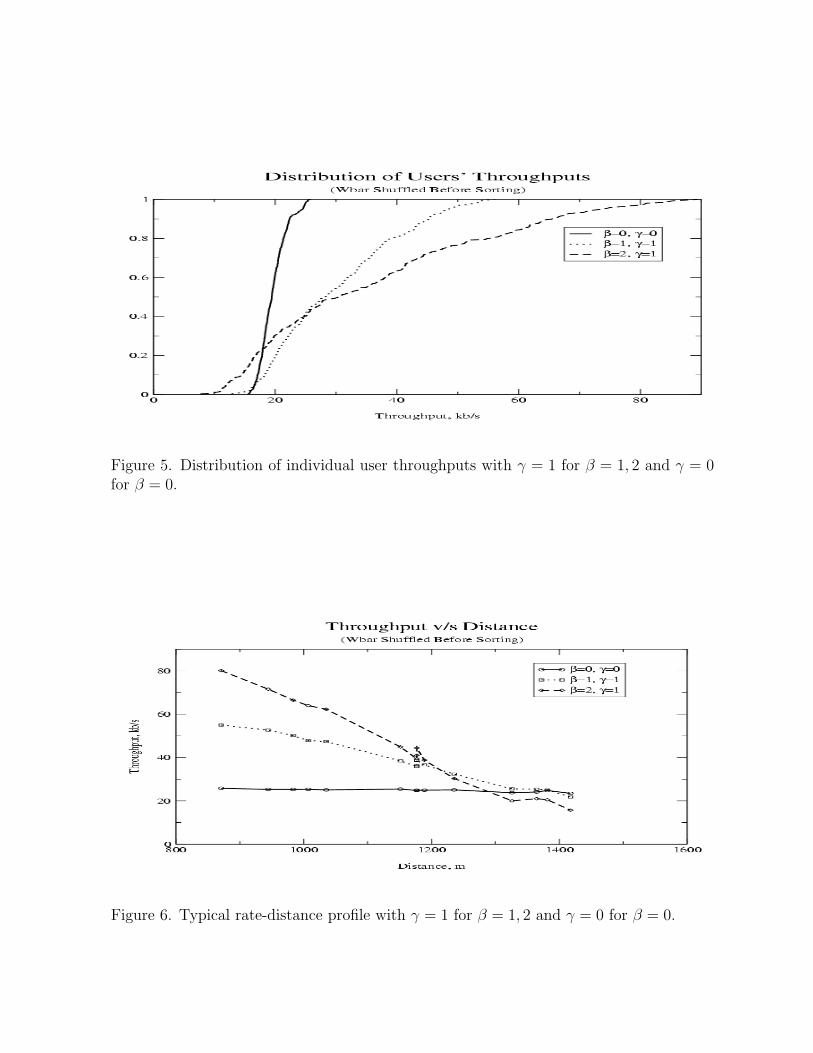
Figure 5. Distribution of individual user throughputs with γ = 1 for β = 1, 2 and γ = 0for β = 0.

Figure 6. Typical rate-distance profile with γ = 1 for β = 1, 2 and γ = 0 for β = 0.