civl - 7904/8904 - civil engineering · model calibration (1) in order calibrate any traffic stream...
TRANSCRIPT
T R A F F I C F L O W T H E O R Y
L E C T U R E - 2
CIVL - 7904/8904
Agenda for Today
Review of last lecture
Field observations
Examples of four highways
Various Flow Models
Calibration of Flow Models
Field Observations (1)
The relationship between speed-flow-density is important to observe before proceeding to the theoretical traffic stream models.
Four sets of data are selected for demonstration
High speed freeway
Freeway with 55 mph speed limit
A tunnel
An arterial street
High Speed Freeway
Figure 10.3

High Speed Freeway (1)
This data is obtained from Santa Monica Freeway (detector station 16) in LA
This urban roadway incorporates
high design standards
Operates at nearly ideal conditions
A high percentage of drivers are commuters who use this freeway on regular basis.
The data was collected by Caltrans

High Speed Freeway (2)
Measurements are averaged over 5 min period
The speed-density plot shows
a very consistent data pattern
Displays a slight S-shaped relationship

High Speed Freeway: Speed-Density
Uniform density from 0 to 130 veh/mi/lane
Free flow speed little over 60 mph
Jam density can not be estimated
Free flow speed portion shows like a parabola
Congested portion is relatively flat

High Speed Freeway: Flow-Density
Maximum flow appears to be just under 2000 veh per hour per lane (vhl)
Optimum density is approx. 40-45 veh/mile/lane (vml)
Consistent data pattern for flows up to 1,800 vhl
High Speed Freeway: Flow-Speed
Consistent data pattern for flows up to 1,800 vhl
Optimum speed is not well defined
But could range between 30-45 mph
Relationship between speed and flow is not consistent beyond optimum flow

Break-Out Session (3 Groups)
Find out important features from
Figure 10.4
Figure 10.5
Figure 10.6

Difficulty of Speed-Flow-Density Relationship (1)
A difficult task
Unique demand-capacity relationship vary
over time of day
over length of roadway
Parameters of flow, speed, density are difficult to estimate
As they vary greatly between sites

Difficulty of Speed-Flow-Density Relationship (2)
Other factors affect
Design speed
Access control
Presence of trucks
Speed limit
Number of lanes
There is a need to learn theoretical traffic stream models

Individual Models
Single Regime model Only for free flow or congested flow
Two Regime Model Separate equations for
Free flow Congested flow
Three Regime Model Separate equations for
Free flow Congested flow Transition flow
Multi Regime Model

Single Regime Models
Greenshield’s Model
Assumed linear speed-density relationships
All we covered in the first class
In order to solve numerically traffic flow fundamentals, it requires two basic parameters
Free flow speed
Jam Density
𝑢 = 𝑢𝑓 −𝑢𝑓
𝑘𝑗∗ 𝑘

Single Regime Models: Greenberg
Second regime model was proposed after Greenshields
Using hydrodynamic analogy he combined equations of motion and one-dimensional compressive flow and derived the following equation
Disadvantage: Free flow speed is infinite
𝑢 = 𝑢𝑓 ∗ 𝑙𝑛𝑘𝑗
𝑘
Single Regime Models: Underwood
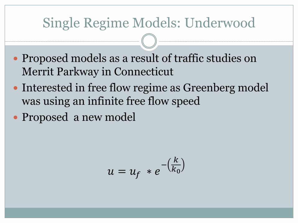
Proposed models as a result of traffic studies on Merrit Parkway in Connecticut
Interested in free flow regime as Greenberg model was using an infinite free flow speed
Proposed a new model
𝑢 = 𝑢𝑓 ∗ 𝑒−
𝑘𝑘0

Single Regime Models: Underwood (2)
Requires free flow speed (easy to compute)
Optimum density (varies depending upon roadway type)
Disadvantage
Speed never reaches zero
Jam density is infanite
Single Regime Models: Northwestern Univ.
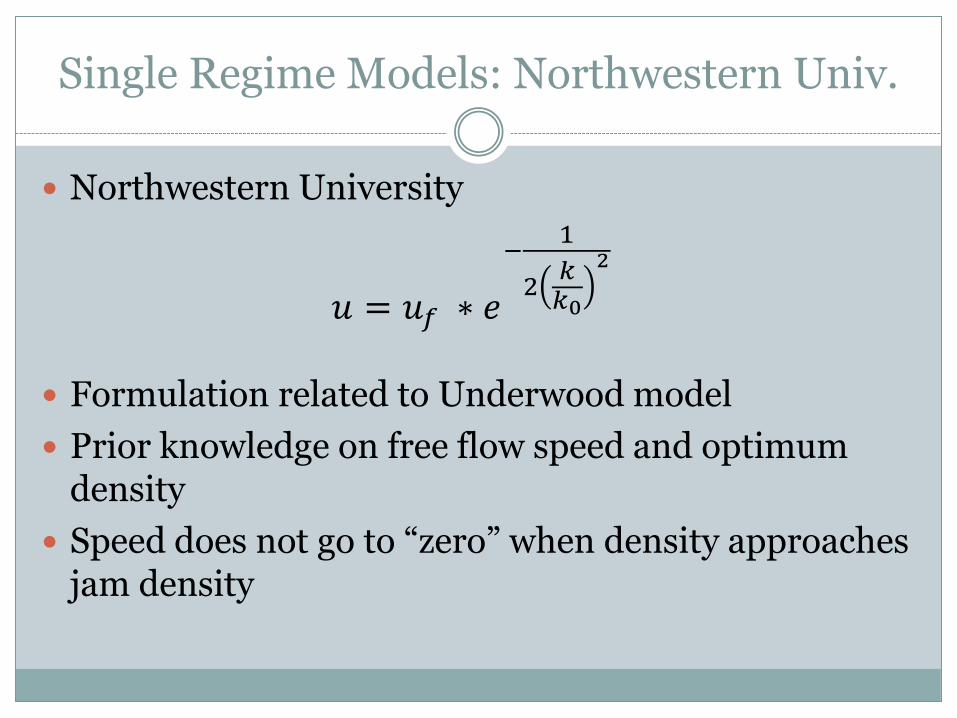
Northwestern University
Formulation related to Underwood model
Prior knowledge on free flow speed and optimum density
Speed does not go to “zero” when density approaches jam density
𝑢 = 𝑢𝑓 ∗ 𝑒
−1
2𝑘𝑘0
2

Single Regime Model Comparisons (1)
All models are compared using the data set of freeway with speed limit of 55mph (see fig. 10.4)
Results are shown in fig. 10.7
Density below 20vml
Greenberg and Underwood models underestimate speed
Density between 20-60 vml
All models underestimate speed and capacity
Single Regime Model Comparisons (2)
Density from 60-90 vml
all models match very well with field data
Density over 90 vml
Greenshields model begins to deviate from field data
At density of 125 vml
Speed and flow approaches to zero

Single Regime Model Comparisons (3)
Flow Parameter
Data Set Greenshields Greenberg Underwood Northwestern
Max. Flow (qm)
1800-2000
1800 1565 1590 1810
Free-flow speed (uf)
50-55 57 --inf.. 75 49
Optimum Speed (k0)
28-38 29 23 28 30
Jam Density (kj)
185-250 125 185 ..inf.. ..inf..
Optimum Density
48-65 62 68 57 61
Mean Deviation
- 4.7 5.4 5.0 4.6

Multiregime Models (1)
Eddie first proposed two-regime models because
Used Underwood model for Free flow conditions
Used Greenberg model for congested conditions
Similar models are also developed in the era
Three regime model
Free flow regime
Transitional regime
Congested flow regime

Multiregime Models (2)
Multiregime Model
Free Flow Regime
Transitional Flow Regime
Congested Flow Regime
Eddie Model 𝑢 = 54.9𝑒−𝑘
163.9
(𝑘 ≤ 50)
NA 𝑢 = 26.8𝑙𝑛
162.5
𝑘
(𝑘 ≥ 50)
Two-regime Model 𝑢 = 60.9 − 0.515𝑘
(𝑘 ≤ 65)
NA 𝑢 = 40 − 0.265𝑘
(𝑘 ≤ 65)
Modified Greenberg Model
𝑢 =48
(𝑘 ≤ 35)
NA 𝑢 = 32𝑙𝑛
145.5
𝑘
(𝑘 ≥ 35)
Three-regime Model
𝑢 = 50 − 0.098𝑘
(𝑘 ≤ 40)
𝑢 = 81.4 − 0.91𝑘
(40 ≤ 𝑘 ≤ 65)
𝑢 = 40 − 0.265𝑘
(𝑘 ≥ 65)
Multiregime Models (3)
Challenge
Determining breakeven points
Advantage
Provide opportunity to compare models
Their characteristics
Breakeven points

Summary
Multiregime models provide considerable improvements over single-regime models
But both models have their respective
Strengths
weaknesses
Each model is different with continuous spectrum of observations

Model Calibration (1)
In order calibrate any traffic stream model, one should get the boundary values,
free flow speed () and jam density ().
Although it is difficult to determine exact free flow speed and jam density directly from the field, approximate values can be obtained
Let the linear equation be y = ax +b; such that is
Y denotes density (speed) and x denotes the speed (density) .

Model Calibration (2)
Using linear regression method, coefficient a and b can be solved as

Example
For the following data on speed and density, determine the parameters of the Greenshields' model. Also find the maximum flow and density corresponding to a speed of 30 km/hr.
k v
171 5
129 15
20 40
70 25

Model Calibration
x(k) y(v)
171 5 73.5 -16.3 -1198.1 5402.3
129 15 31.5 -6.3 -198.5 992.3
20 40 -77.5 18.7 -1449.3 6006.3
70 25 -27.5 3.7 -101.8 756.3
390 85 -2947.7 13157.2
*