Civil Service Reforms:Evidence from U.S. Police Departments

Arianna Ornaghi∗

July 2, 2019

Abstract

Does reducing politicians’ control over public employees’ hiring and firing improve bureau-

cratic performance? I answer this question exploiting population-based mandates for U.S.

municipal police department merit systems in a regression discontinuity design. Merit system

mandates improve performance: crime rates are lower in departments operating under a merit

system than in departments under a spoils system. Changes in resources or police officers’

characteristics do not drive the effect, but I provide suggestive evidence that the limitations to

politicians’ ability to influence police officers are instead important.

JEL codes: H83, M51

∗I am extremely grateful to Daron Acemoglu, Claudia Goldin, and Ben Olken for their invaluable advice andguidance throughout this project. I also thank Enrico Cantoni, Mirko Draca, Daniel Fetter, John Firth, LudovicaGazze, Daniel Gross, Sara Heller, Nick Hagerty, Greg Howard, Peter Hull, Donghee Jo, Gabriel Kreindler, MattLowe, Rachael Meager, Manisha Padi, Bryan Perry, Otis Reid, Frank Schilbach, Mahvish Shaukat, Cory Smith,Marco Tabellini and seminar participants at the MIT Political Economy lunch, the Harvard Economic History lunch,Arizona State University, IIES, Bank of Italy, EIEF, University of Warwick, Barcelona GSE Summer Forum, andthe PSE Conflict Workshop for their comments and suggestions. This research was conducted while the authorwas Special Sworn Status researcher of the U.S. Census Bureau at the Center for Economic Studies. Research re-sults and conclusions expressed are those of the author and do not necessarily reflect the views of the Census Bu-reau. This paper has been screened to ensure that no confidential data are revealed. Correspondence: Arianna Or-naghi, Department of Economics, University of Warwick, Social Sciences Building, Coventry CV4 7AL, UK. Email:A.Ornaghi@warwick.ac.uk.

1

1 Introduction

Bureaucracies are a key component of state capacity. As policy implementers, they translate policychoice into outcomes and affect a state’s ability to provide public goods. We know both from directexperiments (e.g. Chong et al.Chong et al., 20142014) and expert surveys (e.g. La Porta et al.La Porta et al., 19991999; Hyden et al.Hyden et al.,20032003; Kaufmann et al.Kaufmann et al., 19991999) that there is a high degree of variation in bureaucratic performance.Why are some bureaucracies effective while others fail? According to a long tradition in the socialsciences, the first order answer to this question is whether or not politicians control the hiring andfiring of public employees. There is no consensus, however, on the effect that politicians’ controlhas on performance.

Historically, the entire American public administration was characterized by a spoils system inwhich politicians were free to hire and fire bureaucrats as they saw fit. In 1829, President AndrewJackson justified the system on grounds of increased responsiveness: "More is lost by the longcontinuance of men in office than is generally to be gained by their experience" (as quoted inWhiteWhite, 19541954, p. 347). By the end of the 19th century, however, the opposite view – that meritsystems insulating bureaucrats from politics were necessary to give public employees long termincentives and foster expertise through reduced turnover and improved recruitment – had becomemore prominent. Reforms professionalizing the bureaucracy were first introduced at the federallevel in the 1880s and soon started diffusing at lower levels of government. Nevertheless, thedebate on whether politicians’ control improved performance was by no means closed. Whenthe Supreme Court in the late 1970s discussed whether dismissals for political reasons violatedthe First Amendment, the decision was in support of merit systems, but the dissenting opinion ofJustice Stewart clearly supported a return to spoils systems: "Patronage serves the public interestby facilitating the implementing of policies endorsed by the electorate."

Whether merit systems improve performance depends on the trade-off between expertise and re-sponsiveness, and is ultimately an empirical question. Evaluating the trade-off, however, hasproven to be difficult. When bureaucratic organizations are defined at the country level, their effectis confounded by other country-specific factors. When within-country variation exists, endogenousadoption complicates the identification of causal effects. In addition, finding direct measures ofbureaucratic performance can be challenging. The principal contribution of this paper is to providewell-identified causal evidence of the effect of bureaucracy professionalization on a credible set ofperformance measures.

The setting is that of municipal police departments in the United States. In particular, I contrastthe performance of police departments operating under a spoils system with that of departmentsin which a merit system was exogenously introduced. Under a spoils system, politicians were freeto hire and fire police officers as they saw fit. Under a merit system, the authority to appoint, pro-

2

mote and dismiss officers was taken from the mayor and given to a semi-independent civil servicecommission. Hiring and promotion decisions had to follow the results of formal examinations anddismissals were only permitted for just cause.

The first cities to establish merit systems, Albany, Utica and Yonkers (NY), did so in 1884. How-ever, it took a long time for the reform to diffuse at the local level, especially as far as smallermunicipalities were concerned. As late as in the mid-1970s, only 20% of police departments incities with fewer than 10,000 inhabitants had a merit system to hire their police officers.1,2

There is a high degree of variation in how merit systems were introduced at the local level. Thispaper focuses on states with population-based mandates for police department merit systems. Themandates operated in the following way. When the state legislation was first passed, all municipal-ities with population above the threshold in the latest available census were mandated to introducea merit system. At the following censuses, previously untreated municipalities that had grownabove the lower limit also became subject to the mandate and were required to introduce a meritsystem for their police department. Municipalities below the threshold were allowed to introducea merit system at any time.

Whenever a population census was taken, treatment was assigned to all previously untreated mu-nicipalities above the cutoff. As a result, each census defines a separate experiment in which theeffect of the mandate can be estimated using a standard cross-sectional RD design comparing mu-nicipalities just above and just below the threshold. For the causal effect of the mandate to beidentified, municipalities just above and just below the threshold must be comparable. I validatethe assumption by showing that the density of the running variable is smooth at the discontinuityand that municipality characteristics are balanced at baseline.

My main objective is to study how the introduction of merit systems affected the performanceof police departments. I proxy for police performance using crime rates, defined as crimes per100,000 people. The data are from the Uniform Crime Reports (UCRs) published by the FederalBureau of Investigation. UCRs are available at the individual department level only starting from1960. At the end of the 1970s, two U.S. Supreme Court decisions extended protections from polit-ical dismissals to all public employees regardless of municipality size, substantially changing whatit meant to be under a merit system as opposed to a spoils system. The main analysis focuses on the1960 to 1980 period, and exploits variation in treatment status from the 1970 census experiment.

My evidence indicates that merit system mandates improved police performance. In the first tenyears after a municipality became subject to the mandate, the crime rate was 45% lower in munic-

1Merit systems covered all employees in the largest cities but were restricted to members of police and fire depart-ments in the vast majority of municipalities.

2Author’s calculations based on data from Ostrom et al.Ostrom et al. (19771977).

3

ipalities just above the threshold relative to municipalities just below. The result is not explainedby pre-existing differences: there was no discontinuity in the outcome before the introduction ofmerit systems. The effect was gradual over time, and stabilized after four to five years. Interest-ingly, the effect was driven by a decline in the property crime rate as opposed to the violent crimerate: it appears that police officers under spoils and merit systems prioritized different types ofcrimes. Finally, to support the interpretation that merit system mandates improved performance,I show that the clearance rate for violent crimes, defined as crimes cleared by arrest over numberof crimes, also experienced an increase, suggesting that police officers under merit systems mighthave become more effective in their investigations.

I test whether the results depend on the choice of sample, specification and estimation technique.The effect of merit systems on the crime rate is not driven by any of the choices made in theestimation and is also robust to running a series of placebo regressions with randomly assignedthresholds. In addition, I argue that it is improbable that the results are driven by other state-specific policies changing at the same threshold as the results are robust to dropping one state atthe time. Finally, I discuss in detail why the results are unlikely to be an artifact of differentialreporting.

The results discussed thus far show the effect of the mandate itself. Protections granted by themandate were enforceable in court from the moment in which the official census counts werepublished, which means that limitations to political influence over police officers were in placefrom when the mandate became binding, independently on whether a civil service commissionwas instituted in the municipality or not. This makes studying the effect of the mandate meaningfulin this setting. Nonetheless, to make the results more credible, I additionally show evidence thatthe mandates did induce municipalities to fully adopt the reform. Unfortunately no systematicdata on merit system adoption exists for the 1970s, but I was able to collect the information fromthe Municipal Codes of a small sample of municipalities. This allows me to provide suggestiveevidence that indeed, the probability of having a full-fledged merit system increased after 1970 inplaces subject to the mandate. In addition, I show formally that this was the case for the only periodin which data on adoption does exist, 1900-1940. Over this time period, merit system mandatesincreased the probability of introducing a civil service commission by 43 percentage points.

I explore three possible channels that might explain how merit systems had a positive effect on per-formance: increases in the resources available to police departments, changes in police officers’characteristics, and reduced political influence. First, I show that merit systems did not influencethe resources available to police departments. There is no discontinuity at the threshold in expendi-tures or employment, which suggests that departments operating under a merit system used similarinputs as departments operating under a spoils system.

4

Second, I find scant evidence that merit systems selected and retained officers with different char-acteristics. In particular, I study the demographic composition of the departments using a noveldataset with individual-level information on police officers that I constructed from the full countmicrodata from the population censuses 1960 to 1980. I show that there were no differences atthe threshold in the age, educational attainment or veteran status of police officers, suggesting thatimproved performance is unlikely to be explained by merit system departments having "better"police officers.

Given that the effect on performance cannot be explained by merit systems increasing resources orattracting police officers with different characteristics, the last channel, increased protection frompolitical influence, is likely to be important. I provide two pieces of evidence supporting this claim.First, I show that states in which the police chief was also under a merit system, and thus arguablywhere political influence was more strongly curtailed, experienced a larger decline in crime rates.Second, I exploit the fact that at the end of the 1970s two Supreme Court decisions extendedprotections from dismissals for political reasons to all municipal employees to provide indirectevidence on the role played by this provision. After 1980, treated municipalities still had to createindependent civil service commissions, but there was no discontinuity in whether employees wereprotected from being fired for political reasons. I find that merit system mandates had no effecton crime rates after 1980, consistent with the hypothesis that the protections from discretionaryfirings that limited political control over police officers were important to explain the result.

This paper contributes to the growing literature on the organization of bureaucracies by providingwell-identified causal evidence on the effect of police departments’ professionalization on a policyrelevant performance measure: crime rates. The main finding that merit system had a positiveeffect on performance is in line with correlational evidence that professionalized bureaucraciestend to be more effective, such as the cross-country comparisons by Evans and RauchEvans and Rauch (19991999) andRauch and EvansRauch and Evans (20002000). The closest work is that of RauchRauch (19951995), who found using a differences-in-differences design that the introduction of U.S. municipal merit systems increased infrastructureinvestment and city growth rates before 1940. I add to this study by substantially improving iden-tification and by investigating an outcome that is a direct measure of bureaucratic performance.With respect to the recent literature that focuses on the role played by selection of bureaucrats onperformance (e.g. Dal Bo et al.Dal Bo et al. (20132013), Ashraf et al.Ashraf et al. (20182018), DeserrannoDeserranno (20182018), WeaverWeaver (20182018),Voth and XuVoth and Xu (20192019)), I show that professionalizing the bureaucracy may have a positive effect evenwhen the composition of the bureaucracy itself is not affected. The proposed explanation that meritsystems had a positive effect by shielding the bureaucracy from political influence is instead in linewith recent evidence documenting the negative effects of political influence on the bureaucracy,including Akhtari et al.Akhtari et al. (20182018), Colonnelli et al.Colonnelli et al. (20182018), XuXu (ForthcomingForthcoming). In addition, the paperadds to existing work on the effect of U.S. federal and state merit systems on political outcomes

5

(e.g. Folke et al.Folke et al., 20112011; Johnson and LibecapJohnson and Libecap, 19941994; UjhelyiUjhelyi, 20142014). Finally, the paper relates tostudies looking at determinants of police performance by providing evidence of the role playedby police organization (e.g. Chalfin and McCraryChalfin and McCrary, ForthcomingForthcoming; Evans and OwensEvans and Owens, 20072007; LevittLevitt,19971997; MasMas, 20062006).

The remainder of the paper is organized as follows. Section 2 presents the background, section3 presents the data, and section 4 discusses the empirical strategy. The main results and theirrobustness are presented in section 5, and evidence on reform adoption in section 6. Section 7discusses potential mechanisms. Section 7 concludes. Additional tables and details are availablein a separate online appendix.3

2 Background

Historical Background

The Wickersham Commission reports, published in 1931, offer a dismal picture of the state ofAmerican policing at the beginning of the 20th century.4 Police departments across the nationwere described as tainted by corruption and incapable of controlling crime. The main culprit wasidentified to be excessive political influence in policing, which made the tenure of executive chiefsand officers alike too short and the selection of personnel with adequate qualifications impossible.In the words of J. Edgar Hoover (19381938): "the real "Public Enemy Number One" against law andorder is corrupt politics." To overcome these issues, the solution proposed was police profession-alization through the establishment of effective merit systems.

The police was just one of the many public organizations under political control. In fact, startingfrom the Jackson Presidency, the entire American bureaucracy was under a full-fledged spoilssystem, where newly elected presidents would substitute office holders nominated in previousadministrations for party loyals (FreedmanFreedman, 19941994). At the height of the spoils system, wholesalereplacement of federal employees was the norm (United States Civil Service CommissionUnited States Civil Service Commission, 19731973),with replacement rates as high as 50% even for postmasters in charge of smaller offices (FowlerFowler,19431943).

By the mid 19th century, however, the discussion of whether the spoils system was the best wayto organize the bureaucracy had begun. The proponents of professionalization saw it as a responseto widespread inefficiencies; those opposing reform were afraid of losing not only political power,but also the support of an aligned bureaucracy. The first civil service reform aimed at profession-alizing public employees, the Pendleton Act, was adopted in 1883. The act created a bipartisan

3The online appendix is available at the following linklink.4The National Commission on Law Observance and Enforcement, also known as the Wickersham Commission,

was created by President Hoover in 1929 with the objective of studying the state of crime and policing and identifyingpossible solutions.

6

Civil Service Commission and introduced competitive examinations for around 10% of federalemployees. Protection from partisan dismissals was established by the end of the 1890s (LewisLewis,20102010). Expansion was swift: by 1920, 80% of federal employees were covered by a merit sys-tem. Contemporaneous testimonies of postmasters and custom collectors report improvements inthe functioning of their agencies following the reform (U.S. Civil Service CommissionU.S. Civil Service Commission, 18841884), andthe consensus is that there was a positive effect on performance (Johnson and LibecapJohnson and Libecap, 19941994 andCarpenterCarpenter, 20052005).

Albany, Utica and Yonkers (NY) were the first cities to adopt a merit system in 1884. Adoptionpicked up again during the Progressive Era, when reformers identified professionalization as thechief remedy for the inefficiency of city hall. The diffusion of the reform, however, was slowerthan at the federal level, and by 1920, fewer than 40% of cities with more than 25,000 inhabitantshad a merit system.

Police departments were one of the principal agencies involved in municipal merit systems, and inmany smaller cities and towns merit systems were actually restricted to police and fire departments.Originally an offshoot of the Progressive movement (FogelsonFogelson, 19771977, p. 44), the professionaliza-tion of the force was at the center of police reform long after the original impetus had subsided. In19541954, O. W. Wilson was still supporting the ideal: "sound personnel management operates on themerit principle that to the best-qualified goes the job - not to the victor belong the spoils."

Merit System Mandates

There was wide variation in the legislative basis of municipal merit systems. In the majority of thecases, the reform was adopted independently by municipalities through ordinance or referendum.This makes studying the effect of merit systems challenging: because introducing the reform wasa political decision taken by those who had to gain (or lose) from it, the timing was likely endoge-nous. In some cases, however, merit systems were introduced by higher levels of government: thispaper focuses on states in which the legislature mandated merit systems for police departments ofmunicipalities above certain population thresholds.

I collected information on state merit system mandates by performing a state-by-state search ofHistorical Statutes and State Session Laws, using secondary sources to locate relevant informa-tion (see Online Appendix B for details on how the search was conducted).5 As Figure IFigure I shows,there are eight states with mandates based on population thresholds, although only six of themeffectively contribute to the estimation (Appendix Table IIAppendix Table II).6 While there were differences in thedetails of the legislation across states, the fundamental features of the reform were the same. When

5Sheriff’s departments were not subject to the same legislation: the entirety of the paper focuses on municipalpolice departments only.

6Because Wisconsin had two different cutoffs based on whether a municipality was incorporated as a village oras a city, I consider Wisconsin villages and Wisconsin cities separately. When the legislation excludes municipalities

7

a merit system was introduced in a police department, the authority over hiring, promotions anddismissals was removed from the mayor and given to a semi-independent civil service commis-sion. Hiring and promotion decisions, not regulated under a spoils system, had to be based on theresults of formal examinations. Police officers, who could be dismissed by the mayor at will undera spoils system, could only be fired for just cause and had access to a formal grievance procedureadministered by the commission.7

When a merit system was introduced, already employed officers were grandfathered in. The pro-visions covered all police officers of lower ranks, but were sometimes extended to the police chief.Finally, civil service commissions were usually nominated by the mayor or by the governing bodyof the city, but overlapping terms and requirements on members’ political affiliations decreased therisk of capture.8

The years of introduction of the reform at the state level range from 1907 to 1969. When thestate legislation was first passed, all municipalities above the population threshold according to thelatest available census had to introduce a merit system for their police department. In all subsequentcensuses, municipalities that had grown above the cutoff also became subject to the mandate andhad to introduce a merit system. In approximately half of the states, the mandate was explicitlybased on the federal population census, whereas in the remaining ones any official municipal, stateor federal census could also be used. Only a few states had penalties for non-compliance, but theprotections given to police officers became binding the moment that the official counts from thecensus were released, and could be challenged in court. Finally, municipalities below the thresholdwere allowed to introduce a merit system through ordinance or referendum at any time. At theend of the 1970s, two U.S. Supreme Court decisions, Elrod v. Burns (1976) and Branti v. Finkel(1980), made dismissals for political reasons illegal for all non-policymaking municipal employeeson grounds of violation of the First Amendment, substantially limiting political influence even inmunicipalities not under a merit system.9

The thresholds are between 4,000 and 15,000: the legislation focused on police departments insmall municipalities. Small town police departments (e.g. departments in municipalities below10,000 people) employed around one civilian and six full-time sworn officers, four of whom had

under specific forms of government (for example, municipalities under a city manager form of government before1933 in Wisconsin), I omit them from the analysis.

7Police unions may also make it hard for an administration to fire police officers. To the extent that there is tomy knowledge no reason why the probability of being unionized should not be smooth across the discontinuity, thisshould not impact my results.

8In five out of nine cases (Arizona, Illinois, West Virginia, Wisconsin cities and Wisconsin villages), the commis-sion was bipartisan, and in two additional states (Iowa and Louisiana), members were required to be non-political.In Montana and Nebraska, members were only required to be citizens of good standing supporting the merit systemprinciple for public administration.

9Elrod v. Burns, 1976, 427 U.S. 347. Branti v. Finkel, 1980, 445 U.S. 518.

8

grade of patrolman, highlighting a limited role for career incentives. They engaged in patrolling,traffic control and early criminal investigations, with limited specialization, and relied on externalsupport for more complex tasks (Falcone et al.Falcone et al., 20022002).10

3 Data

Crime. The crime data are from the Uniform Crime Reports (UCRs) published by the FederalBureau of Investigation. UCRs are compiled from returns voluntarily submitted to the FBI bypolice departments, and are available for individual agencies starting from 1960. They reportmonthly counts of offenses known to the police and cleared by arrest for three property crimes(burglary, larceny-theft, and motor vehicle theft) and four violent crimes (murder and negligentmanslaughter, rape, robbery, and aggravated assault).11 I use UCRs to study crime rates, definedas crimes per 100,000 people, and clearance rates, defined as number of crimes cleared by arrestover total number of crimes.12 Appendix Table IIAppendix Table II presents the descriptive statistics.

Reform adoption. I predict the year in which a municipality became subject to the mandate usingpopulation counts digitized from the official publications of the Census Bureau and informationon state merit system laws. Limited data on adoption are available for the main period of interest,but I was able to collect the year of introduction of the reform for a small number of municipalitiesin the sample from these cities’ Municipal Codes. In addition, I use three surveys conducted bythe Civil Service Assembly of the United States in 19371937, 19401940 and 19431943 to provide evidence onreform adoption for an earlier period.13

Expenditures and employment. Data on expenditures and employment for police departmentsare from the Annual Survey of State and Local Government Finances and the Census of Govern-ments published by the Census Bureau.14 I study total expenditures per 1,000 people and total

10Author’s calculations based on a 1974 survey conducted by Elinor Ostrom (Ostrom et al.Ostrom et al., 19771977). The surveyprovides information on all police departments in a random sample of standard metropolitan areas.

11I clean the data for missing values following the indications reported by MaltzMaltz (20062006), but I do not use his dataimputation procedure. I show that the results are robust to additional data cleaning aimed at identifying outliers in therobustness checks. Online Appendix C reports more details.

12For intercensal years, I linearly interpolate municipal population from the official publications of the CensusBureau. I prefer this to using municipal population reported in UCRs themselves as visual inspection of the datasuggests that the variable presents a high degree measurement error, but I show that this does not impact the mainresults as a robustness check. A crime is considered cleared by arrest if at least one person has been arrested, charged,and turned over for prosecution (FBI websiteFBI website). There is no perfect correspondence between the crimes that are reportedas being cleared in a certain month and the offenses taking place in that month, although most arrests happen close tothe date of the incident. Given that I find large effects on crimes, normalizing by volume is important. Clearance rateshave been used as proxy for performance in the economics of crime literature, for example in McCraryMcCrary (20072007).

13Previous studies using these data include Tolbert and ZuckerTolbert and Zucker (19831983) and RauchRauch (19951995).14The data on expenditures are available at the municipality level starting from 1970, and the data on employment

from 1972. Both datasets cover the universe of municipalities in 1972 and 1977 (from the Census of Government) anda sample of local governments in all other years (from the Annual Survey of State and Local Government Finances).

9

employment per 1,000 people.

Police officer characteristics. I construct a dataset of police departments’ demographic charac-teristics starting from the restricted access full count microdata of the 1960 to 1980 DecennialCensuses.15 I identify police officers using reported occupation, industry and class of worker,and I assign each police officer to the department of the municipality in which they were enumer-ated.16,17

4 Empirical Strategy

The empirical strategy to identify the impact of merit systems exploits population-based mandatesin a regression discontinuity design. The key feature of the setting is that each population cen-sus defines an experiment in which treatment is assigned to all previously untreated ("at risk")municipalities. The causal effect of the reform can be estimated using the following specification:

ymt = β1(distm > 0) + f (distm) + δst + εmt f or m ∈ RS (1)

ymt is outcome y for municipality m and month (or year) t; distm is the population distance to thethreshold (i.e. the running variable); 1(distm > 0) is an indicator for being above the threshold;f (distm) are a set of flexible functions of the running variable; δst are state-month (or year) fixedeffects; and RS is the set of "at risk" municipalities, i.e. all municipalities in the last censusbefore the introduction of the state legislation and previously untreated municipalities in eachcensus experiment thereafter. β estimates the effect of having a mandated merit system and isthe coefficient of interest. The fixed effects are not needed for identification but increase precision.Standard errors are clustered at the municipality level to correct for the correlation induced byincluding the same municipality multiple times in the estimation.

I estimate the results using locally linear regression (Gelman and ImbensGelman and Imbens, 20162016) and a uniformkernel, which is equivalent to estimating a linear regression on observations within the bandwidthseparately on both sides on the discontinuity. I show results for three fixed bandwidths (750,1,000, 1,250) and for an outcome- and sample-specific MSE-optimal bandwidth calculated using

15The microdata are available for every individual who participated in the census, but starting in 1960 work-relatedquestions were only asked in long form schedules, which means that I am effectively using a sample covering 15% to25% of the U.S. population depending on the year.

16Using information on place of work to match police officers to departments is unfeasible because of the coding ofthe data. For the individuals for which I can identify place of work municipality, I can check whether the assumptionis correct. I find that 73% of these police officers work for the department of the municipality in which they reside.

17I validate the procedure comparing the number of police officers in the census with the number I should expect tofind given the long form sampling frame and the number of police officers reported for each department in the Censusof Government. The procedure appears to work quite well. In 1970, for 84% of departments the discrepancy is lowerthan two and for 59% it is lower than one. The error rates are 91% and 63% in 1980.

10

the procedure suggested by Calonico et al.Calonico et al. (20142014). The optimal bandwidth is calculated separatelyfor each outcome and sample after partialling out the fixed effects and allowing for clustering ofthe standard errors following Bartalotti and BrummetBartalotti and Brummet (20162016).

The main effect is estimated pooling all post-treatment observations. The post-treatment periodstarts either in the year of introduction of the mandate at the state level or, for all the followingcensus experiments, in the year of the population census itself. It ends in the year of the follow-ing census.18 As a falsification test, I check that there are no pre-existing discontinuities in theoutcomes by estimating the same specification on pre-treatment observations.

To understand how the effect of the mandate changes over time, I estimate the following RD eventstudy specification:

ymt = ∑σ∈{−5,+10}

βσ1(distm > 0)1(t− c̃ = σ) + ft(distm) + δst

+εmt f or m ∈ RS(2)

ymt is outcome y for municipality m and month (or year) t; distm is the population distance to thethreshold (i.e. the running variable); 1(distm > 0) is an indicator for being above the threshold;1(t − c̃ = σ) is an indicator equal to 1 if σ years have elapsed since treatment (c̃ is treatmentyear for census experiment c); ft(distm) is a set of year specific flexible functions of the runningvariable; δst are state and month (or year) fixed effects; and RS is the set of "at risk" municipalities.βσ estimates the effect of having a mandated merit system for σ years and is equivalent to the RDestimate from a cross-sectional RD that pools all observations measured σ years since treatment.The specification is estimated pooling both pre- and post-treatment observations. Standard errorsare clustered at the municipality level.

The identification assumption is that all factors other than treatment vary continuously at thethreshold. First, municipalities must not sort around the cutoff according to their characteris-tics. I validate the design by testing for discontinuities in the density of the running variable andin baseline covariates. Appendix Figure I Panel AAppendix Figure I Panel A presents the McCraryMcCrary (20082008) test for the 1970census experiment: the density of the running variables shows no discontinuity at the threshold.Supporting the idea that there was no sorting, the figure additionally shows the McCrary test forall census experiments in which treatment was assigned, ranging from 1910 to 2000. Out of theten census experiments, the McCrary test only barely fails for 1980, in line with statistical error.

18I focus on the short-term effect of the mandate because the long-term effect would be confounded by the controlmunicipalities growing above the threshold and being treated in following census experiments. I could estimate longer-term effects by comparing outcomes for places that were just above and just below the threshold in a certain censusand below the threshold in the following one. However, given that most cities experience population growth, I do nothave enough data to estimate such treatment effects.

11

Appendix Table IIIAppendix Table III shows the results of a covariate balance test. The table reports the coefficienton the dummy for being above the threshold for three fixed bandwidths (750, 1,000, 1,250) andan outcome-specific MSE-optimal bandwidth. The outcomes are municipality characteristics mea-sured in the population census in which treatment was assigned. None of the coefficients for the1970 census experiment is statistically different than zero: the places just below the threshold area good control group for those just above. Reassuringly, even if the McCrary test fails for 1980,Appendix Table IIIAppendix Table III shows covariate balance for the same census experiment.

Second, to estimate the causal effect of merit systems, it must also be the case that no other policieschange at the same threshold, a particularly common issue for RD designs based on populationcutoffs (Eggers et al.Eggers et al., 20182018). I provide evidence that it is unlikely that other policies are drivingmy results in the robustness checks section.

5 Effects of Merit System Mandates on Performance

I study the effect of police professionalization on performance by estimating the impact of meritsystem mandates on crime and clearance rates. The analysis uses outcome data for the 1960 to1980 period: crime data are available at the department level starting from 1960, and SupremeCourt decisions extending protections from dismissals for political reasons to all municipal workersaltered the content of the reform at the end of the 1970s.19 Variation in treatment status is from the1970 census experiment.20

The analysis estimates the effect of merit system mandates. Estimating the effect of the mandatesthemselves is meaningful in this setting. Protections against hiring and dismissals for politicalreasons could be challenged in court as soon as the municipality fell under the mandate: man-dates effectively restricted political influence even without the creation of a separate commission.21

Nonetheless, if we define treatment as adoption of a full-fledged merit system, I estimate intentionto treat effects, as there exists limited data on merit system adoption for the 1970s.

19Appendix Table IIAppendix Table II reports descriptive statistics. The increase in sample size between the pre- and post-treatmentperiod is explained by more agencies reporting data to the FBI. I do not restrict the analysis to a balanced samplebecause the estimation is based on within-month comparisons of places above and below the threshold, and I wantto maximize all available data, but I show that restricting the estimation to a quasi-balanced sample does not make adifference in the robustness check section.

20The 1970 census experiment is the only one for which outcome data are available for both the pre- and post-treatment period. The 1960 census experiment has outcome data for the post-treatment period only. As shown inAppendix Table IVAppendix Table IV, police departments in municipalities just above the threshold were more likely to submit data tothe FBI in 1960. This is a potentially interesting outcome as it suggests that police departments under a merit systemhad better record keeping practices. However, it makes it impossible to interpret the results on crime rates, which iswhy I exclude the 1960 census experiment from the analysis.

21Wayne, Nebraska offers an example for this. Even if the municipality had not complied with the mandate by1973, it had to reinstate a chief of police who had been unfairly dismissed by the mayor after a district court ruled hewas entitled to civil service protections even without a commission.

12

I begin by showing descriptively how the crime rate, defined as crimes per 100,000 people, changedover the period from 1965 to 1979 for municipalities that were under a merit system mandate andfor municipalities that were not. Figure IIFigure II shows the mean monthly crime rate by year separatelyfor places above and below the threshold, together with 95% confidence intervals. Over the pe-riod of interest, places both above and below the threshold experienced a stark increase in crimerates, but while places below the threshold kept growing at a steady pace throughout the period,departments that fell under the merit system mandates saw crime rates increase more slowly after1970.

Figure III panel AFigure III panel A shows the visual equivalent of the RD estimates for the crime rate. The panelon the left shows the falsification RD graph estimated on the sample of pre-treatment years (1960to 1969), while the one on the right shows the main RD graph of interest, estimated on post-treatment years (1970 to 1979).22 Outcomes are defined as log crime rates.23 The dots showthe average value of the outcome for different bins of the running variable. The line plots the fitfrom a locally linear regression estimated separately on each side of the discontinuity. State-monthfixed effects are partialled out. The RD graphs show that there was no difference in the crime rateat the discontinuity in the pre-treatment sample. However, after the mandate became effective,municipalities just above the threshold had a lower crime rate than those just below.24

The regression estimates confirm the results. Table ITable I shows the effect of having a mandatedmerit system for three fixed bandwidths and for a MSE-optimal bandwidth separately for the pre-treatment sample (columns 1 to 4) and for the post-treatment sample (columns 5 to 8). Panel Ashows that there was no difference in the crime rate in the pre-period, but municipalities above thethreshold had a lower crime rate in the post-period with respect to those below. The coefficientsare statistically significant at the 5% level, and the results are robust to different bandwidths. The

22Preliminary counts for the population census were published between May and October, which makes the yearwhen the census is taken a transition year. In the baseline estimation, I consider it a post-treatment year. The resultsare unchanged if the post-treatment period is considered as starting in 1971.

23The log transformation drops observations with 0 crimes, but I show in Appendix Table VAppendix Table V that this does not makea difference: using crime rates, inverse hyperbolic sine of crime rates, crime counts and log of crime counts gives thesame results. This is not surprising to the extent that in fewer than 2% of the observations of municipalities within a1,250 bandwidth in the post period is the monthly crime rate equal to zero. The negative coefficient in the pre-periodfor the inverse hyperbolic sine specification can potentially be explained by the relatively low data quality in the veryfirst few years of the UCR program. Even extensively cleaning the data, understanding whether a zero observation is atrue zero or a missing datum remains a challenging task (MaltzMaltz, 20062006). Considering all zero (total crime) observationsas missing in the pre-period reduces the size of the coefficient. This is less of an issue in the post-treatment period,where zero observations are significantly fewer and the quality of the data appears to have improved. In addition,the negative coefficient could be explained by anticipation effects (see below for details): excluding years in thepre-treatment period when anticipation is likely also reduced the size of the coefficient.

24Given that I am partialling out state-month fixed effects and crime rates are significantly increasing over time, itis not possible to compare levels across the RD graph of the pre- and post-treatment period. The change over time inthe outcome is more correctly inferred from Figure IIFigure II: both municipalities above and below the threshold see highercrime rates over the period, but the increase is slower for places above the threshold.

13

magnitude of the effect is large: looking at the estimates for places within a 1,000 bandwidth fromthe threshold, the coefficient shows a 45% reduction in crime rates for treated places in the firstten years after the reform was introduced. The median municipality in the control group withina 1,000 bandwidth from the threshold has 10 total crimes per month, which means that munici-palities under merit system mandates experienced 4.5 fewer total crimes per month. To put thisin perspective, this is equivalent to the department hiring between 2 to 3 additional police offi-cers according to the crime-police elasticities for municipalities of similar size reported in MelloMello(20182018).

To the extent that unobservables vary continuously at the threshold and there are no pre-treatmentdifferences in the socio-economic composition of control and treated municipalities, the effectis unlikely to be explained by other external factors, suggesting that indeed the result must beexplained by changed police behavior. Overall, it appears that merit system mandates improvedpolice performance.

Heterogeneous effects over time. To understand how the effect of the mandate changed overtime, Figure III panel BFigure III panel B shows the βσ coefficients from the event study specification together with95% confidence intervals.25 The graph on the left shows that the effect is gradual over time andis statistically significant starting two to three years after treatment was assigned in 1970. Noneof the coefficients in the pre-period is statistically significant, but the point estimates are negative,and start becoming larger in magnitude two to three years before treatment. This is potentiallyconcerning, as it may point to pre-existing differences in crime rates. However, it is important tonote that the negative coefficients could be explained by early adoption of merit systems, whichwould not invalidate the design.

I provide evidence that this is indeed the case by estimating the event study separately for states inwhich early adoption was more or less likely. In particular, I exploit the fact that in four states inmy sample (Illinois, Montana, Nebraska and West Virginia), the mandate was based on populationmeasured in any official municipal, state or federal census. In these states, it is likely that themandate became effective before the federal census was released, as the actual population of amunicipality grew above the threshold and an official census was taken. On the contrary, thereshould be no anticipation where the mandate was explicitly based on the federal population censusonly. Reassuringly, the graph on the right shows the presence of an anticipation effect only in stateswhere the mandate was based on any official census. When I focus on states where the mandatewas strictly based on the federal census only, there is no difference in crime rates until 1972 - ifanything, the coefficients are positive, although not significantly different than zero. The decline

25Different from differences-in-differences event study specifications, there is no omitted category because themodel never gets fully saturated and the omitted category is constituted by control municipalities in each experiment.

14

is gradual at first, but remains constant in magnitude after a few years.26

Heterogeneous effects by type of crime. To explore whether police officers under spoils and meritsystems prioritize different types of crime, Table I Panel BTable I Panel B estimates the main regression separatelyfor the property and the violent crime rate (see Appendix Figure IIAppendix Figure II for the respective RD and eventstudy graphs). The effect appears to be entirely driven by the property crime rate: places abovethe threshold had a similar property crime rate as places below the threshold in the pre-period, butlower property rates after the mandate became effective. Merit systems had no effect on the violentcrime rate: there is no discontinuity at the threshold, and the coefficient for being subject to a meritsystem mandate is never significantly different than zero.27 This can be potentially rationalizedby police officers under spoils systems over-prioritizing violent crimes, maybe because they aremore relevant for politicians or more likely to be in the news, and merit system mandates inducingpolice officers to reallocate effort towards activities with positive marginal returns. Given that thedecrease in the property crime rate comes at no cost for the violent crime rate, I interpret this resultas again supporting evidence that merit system mandates improved police performance.

Reporting bias. For the interpretation of increased police performance to hold, it must be the casethat the decline in crime rates represents a true decline in crime, and not just in crime statistics:there must be no differential reporting at the threshold. I provide three pieces of evidence that thisis the case, related to different ways in which differential reporting may arise. First, citizens whoexperience a crime may not report it or, even if the crime is reported, the police may fail to create arecord for it. Misreporting at this stage is less likely for crimes that involve insured goods such asburglaries and vehicle thefts, as insurance companies often would not honor theft claims withouta police report. Appendix Table VIIIAppendix Table VIII shows that merit systems had a negative effect both on theburglary and vehicle theft rate and on the larceny rate, although the coefficients on burglary andauto theft are not significant for all bandwidths. Second, after a record is created, it can be alteredto distort crime incidents reported to the FBI. In particular, as discussed in Mosher et al.Mosher et al. (20102010),an offense can be downgraded to a non-index crime or it can be reported as unfounded. The fact

26A true anticipation effect is also consistent with the coefficient in the pre-treatment sample in Table ITable I being neg-ative for some bandwidths, although always smaller in magnitude than the effects I estimate in the post-treatmentsample and never statistically significant. In fact, as shown in Appendix Table VIAppendix Table VI, estimating the main specificationdropping pre-treatment years in which the anticipation effect is likely gives coefficients that are smaller in magnitudeand, again, never statistically significant.

27Violent crimes are a rare event. In the post-treatment period, only 37% of observations correspond to months witha positive violent crime rate, as opposed to 98% of observations corresponding to months with a positive propertycrime rate. As a result, we might be interested in understanding whether merit systems affect the extensive marginof violent crimes, even if the main analysis shows no effect on the violent crime rate conditional on it being positive.Appendix Table VIIAppendix Table VII shows the effect of merit system mandates on the probability of reporting at least one violentcrime in a month. The coefficient in the post-treatment period is negative, but only statistically significant for smallerthresholds. I interpret this result as confirming that most of the effect was indeed through changes in the propertycrime rate.

15

that I find similar effects across crime types is reassuring as not all crimes can be downgraded aseasily.28 Third, the department may fail to submit a report to the FBI as participation in the UCRprogram is voluntary. I can exclude the possibility since, as Appendix Table IXAppendix Table IX shows, there isno discontinuity at the threshold in the probability of submitting crime data for any given month.Overall, it seems unlikely that the effects are driven by differential crime reporting.

Effects on clearance rates. Finally, to support the interpretation that merit system mandates didimprove police performance, I explore what happened to a different set of outcomes that alsoproxy for police performance: clearance rates, defined as the number of crimes cleared by arrestover total crimes.29 Given that probability of arrest varies starkly by type of crime - clearance ratesfor property crimes are around 20% whereas clearance rates for violent crimes are much higher, ataround 60% - and merit systems affected crime composition, I estimate effects separately by typeof crime. Table I Panel CTable I Panel C shows no difference in the property crime clearance rate, either pre- orpost-treatment. There was no difference in the violent crime clearance rate in the pre-treatmentsample, but in the post-period the coefficient is positive and statistically significant at the 5% level:the violent crime clearance rate is 0.10 points higher in police departments in municipalities justabove the threshold than in those just below (see Appendix Figure IIIAppendix Figure III for the respective RD andevent study graphs). Most property crimes never get cleared in the first place, as it is less likelythat the victim can identify the suspect, so there is limited chance of improved investigations ofproperty crimes to lead to an arrest: it is not surprising that increased effort by police officerswould be reflected in the violent crime clearance rate only. Overall, it appears that the decline incrime was driven by a combination of deterrence, i.e. an increase of expected cost of crime due topolice actions, and incapacitation, i.e. a decrease in the number of potential offenders because ofincreased arrest rates.

Robustness Checks

In this section, I show that my results are robust to a number of potential concerns. Figure IVFigure IVshows the coefficient for the dummy for being above the threshold, together with 95% confidenceintervals, for different samples, specifications, and estimation techniques. The relevant comparisonis whether each coefficient is different than the one estimated using the baseline specificationreported at the top of each graph.30

28In particular, larcenies below $50 are not an index crime, which makes them particularly susceptible to the is-sue. Unfortunately, counts of unfounded offenses are not reported before 1978 so I cannot test directly whether thisdimension is affected.

29I interpret clearance rates as a proxy of performance to the extent that they should correlate with police officers’investigative efforts. Unfortunately, it is not possible to link the arrest data to the ultimate outcome in the judicialsystem for this time period.

30Appendix Figure IVAppendix Figure IV shows the same graphs separately by type of crime and for clearance rates. The equiva-lent tables are Appendix Table XaAppendix Table Xa, Appendix Table XbAppendix Table Xb and Appendix Table XcAppendix Table Xc. I only show estimates for a 1,000bandwidth for clarity, but the estimates for the full set of bandwidths can be found in the Online Appendix.

16

Robustness to data cleaning. To begin with, Figure IV Panel AFigure IV Panel A focuses on data cleaning. First,it shows that the main result is robust to dropping outliers in the crime data identified using a pro-cedure similar to Evans and OwensEvans and Owens (20072007), Chalfin and McCraryChalfin and McCrary (ForthcomingForthcoming) and MelloMello (20182018)(for more details, see Online Appendix C). The result is not driven by especially high - or low -crime observations, that could possibly just be data errors. Second, it shows that using smoothedUCR population as opposed to linearly interpolated population from the census to define crimerates also does not make a difference.

Robustness to using yearly data. The core analysis uses monthly data to exploit all the variationthat is available, which is especially important since I am dealing with a relatively small sampleand I want to maximize power. However, using yearly crime data does not make a difference: thecoefficient estimate is the very similar in magnitude, and still significant at the 5% level.

Robustness to population dynamics. A potential concern is that places right above the thresholdhave different population dynamics with respect to places just below, and the estimates are pickingup the fact that crime rates vary by population. Figure IV Panel AFigure IV Panel A shows that population dynamicsdo not explain my findings: the main result survives controlling for 1980 population and droppingplaces that experience a population growth rate from 1970 to 1980 above 20%.

Effect not driven by sample composition. Finally, I show that the main result is not due tochanges in the composition of municipalities above and below the threshold. The result is un-changed if I restrict the analysis to a quasi-balanced sample of municipalities reporting crime dataat least half of the months, corresponding to 85% of the municipalities and 88% of the observa-tions). Taken together with the fact that the probability of submitting a report was not differentialat the threshold, this is reassuring that the results are not entirely driven by a few very low-crimemunicipalities above the threshold starting reporting after 1970. But, one might still worry aboutthe effect being driven by different municipalities reporting above and below the threshold in thepre- and post-treatment periods. I try to assuage this concern with two specifications. First, theresult is robust to controlling for a host of baseline municipality characteristics. Second, I estimatea difference-in-difference specification that includes municipalities fixed effect, thus allowing meto estimate the effect off of changes in crime rates for the same municipality before and afterthe mandates become binding. The coefficient on the crime rate in this differences-in-differencesspecification is smaller in magnitude but still significant at the 10% level.31

Robustness to two-way clustering Clustering standard errors at the municipality and county-year31This specification is similar to equation (1), but includes municipality fixed effects and allows the flexible con-

trols of the running variable to vary by year. The coefficient reported is from an interaction of an indicator variablefor being above the threshold and an indicator variable for being in the post-period. It is estimated on the 1960 to1979 period. I prefer equation (1) as my baseline specification because, as discussed in Lee and LemieuxLee and Lemieux (20102010) andHinnerich and Pettersson-LidbomHinnerich and Pettersson-Lidbom (20142014), municipality fixed effects are not necessary for identification but introducemore restrictions.

17

level to allow for errors to be correlated for places that are close to each other does not make adifference.

Robustness to overlapping legislation. For RD designs to recover causal effects of a certainpolicy, it must be the case that no other policies change at the same threshold. Appendix Table IAppendix Table Ishows the results of state-by-state search for such policies.32 Most of the states have at least onelegislative provision that implies a policy discontinuity at the same cutoff, although most of themare not police related. However, no single provision is the same across states, which means that Ican provide evidence that no other policy explains the effect by showing that the results are robustto dropping one state at a time. Were the effects driven by any of the other policy discontinuities,they should disappear once the state is dropped. Figure IV Panel BFigure IV Panel B shows the result of this exercise.The magnitude of the coefficient is stable across samples. The stability of the coefficient suggeststhat no other policy has a strong enough effect to bias the results or, in other words, collinearpolicies satisfy an "ignorability" assumption as defined in Eggers et al.Eggers et al. (20182018). Moreover, giventhat different states had different thresholds, this exercise also points towards the results not beingdriven by potential changes in population-based federal policies, such as eligibility for federalgrants.

Robustness to estimation. Finally, Figure IV Panel CFigure IV Panel C shows that the specific estimation tech-nique used does not matter for the results. First, I show robustness to using a triangular and anEpanechnikov kernels. The main result is not affected, although the coefficient is larger in magni-tude. Second, I estimate the main specification using locally quadratic regression and locally cubicregression with a uniform kernel. The result is robust to using a locally quadratic regression, butwhen a cubic polynomial is used the coefficient is not significant, albeit similar in magnitude. Inaddition, the results are robust to dropping the state-month fixed effects and allowing the runningvariable to vary flexibly both by census and by outcome year as in the event study specification.33

Placebo thresholds. As an additional robustness check, I engage in a placebo exercise in whichI randomly assign thresholds to states.34 Figure VFigure V shows the distribution of the estimated coeffi-

32Overlapping legislation was identified by searching for the threshold in historical State Statutes and State SessionLaws. More details are available in Online Appendix C.

33The discussion of the robustness checks has focused on the effect on the crime rate in the post-period, but ro-bustness separately for property and violent crime and clearance rates are also reported in Appendix Figure IVAppendix Figure IV andAppendix Table XaAppendix Table Xa, XbXb and XcXc. Overall, the result on the property crime rate tracks that of the total crime rate, whilethe result on the violent crime clearance rate is less robust. The result that there are no pre-treatment differences is alsorobust to the different choices of sample, specifications and estimation, with one exception. When the median house-hold income is included among the baseline municipality characteristics, the pre-treatment coefficient estimate in theproperty crime rate analysis is negative and statistically significant, although smaller in magnitude than the coefficientestimate for the post-treatment period under the same specification (Online Appendix Tables 6a and 6b). In all otherspecifications, in the few cases in which the coefficient is significant, it is always so at the 10% level and never for allthresholds.

34In particular, I take 999 random permutations of the relevant thresholds for the 1970 census experiment (15,000,

18

cients resulting from the placebo regressions. Out of 999 regressions, only 23 display a treatmenteffect that is more extreme than the one of the baseline specification, which suggests that the resultis not just a feature of population or crime dynamics around the relevant population cutoffs.35

6 Merit System Adoption

Contemporaneous evidence. Unfortunately, no systematic data on adoption of merit systems ex-ists for the 1970s. Municipal Codes do sometime report the date in which the reform was adopted,and I was able to collect information for 53 municipalities out of the 139 within a 1250 bandwidthfrom the threshold.36 The small sample, especially above the threshold, does not allow me to es-timate a proper first stage, but I use the data to provide suggestive evidence that mandates wereindeed effective at inducing municipalities to adopt merit systems. Figure VFigure V shows rate of adop-tion by year separately for municipalities above and below the threshold. The figure allows meto make two important points. First, municipalities above the threshold did indeed adopt aroundthe time they fell under the mandate. Given that these were small municipalities, it makes sensethat once the department introduced the reform, both current and perspective police officers wouldhave been aware of it, which strengthens the credibility of the main results. Second, the vast ma-jority of municipalities below the threshold did not have a merit system by the end of the decade.37

Given the effect on crime, it might be puzzling that not all municipalities introduced the reform.If politicians prioritize violent crimes, which are not affected by the reform, they might lack theincentive to adopt. Moreover, these reforms implied a costly administrative reorganization, whichmight further discourage adoption.38

Historical evidence. In addition, thanks to the fact that some states introduced the mandates in

10,000, 8,000, 7,000, 5,500, 5,000, and 4,000) and assign thresholds to states according to these permutations, underthe constraint that no state is assigned its real threshold. I keep the initial year of introduction of the reform constant,but I ignore instances in which the threshold was lowered (each state is assigned one threshold only). I then identifythe correct risk set, running variable and treatment status to municipalities using the placebo threshold, and re-estimatethe baseline specification.

35Alternatively, only 18 regressions give a t-statistics higher than 1.96.36Bostashvili and UjhelyiBostashvili and Ujhelyi (20182018) note that an important empirical challenge to study merit systems is to collect

information on reform adoption for a large number of jurisdictions. To the best of my knowledge, the data is notreported in any state or national survey or publication, and the introduction of merit systems was not systematicallyreported in local newspapers. In addition, in a phone survey of a small sample of these municipalities, municipalofficials would almost never be able to provide the information when not reported in the Municipal Code.

37The figure shows a limited anticipation effect in the 1970 census experiment, which can be explained by munic-ipalities for which I have adoption information mainly being from states with mandates based on the federal census.Splitting the sample of municipalities below the threshold into those that fell under the mandate in 1980 and those thatdid not, as in Appendix Figure VAppendix Figure V, shows evidence of an anticipation effect for the 1980 census experiment, for whichI have information for municipalities in all states.

38This stance is clearly exemplified in the answer given by Eugene Smith, a candidate for the 1975 mayoral electionof Elwood, Indiana, when asked whether he was planning to introduce a merit system for the fire and police depart-ments: "Merit systems for police and firemen for the small number of employed on our forces would tend to causemore dissention rather than improved performance."

19

the first half of the 20th century, I provide evidence that the legislation was effective at inducingmunicipalities to adopt merit systems for the one period for which systematic data on adoption doesexist, 1900-1940. I proxy for the presence of a full-fledged merit system using year of introductionof a civil service board, available from a census of civil service agencies. Table IITable II shows thecoefficient on the dummy for being above the threshold before and after treatment. Given that theoutcome data are available until 1940, the first stage exploits variation in treatment status from the1900, 1910, 1920 and 1930 census experiments.39

There is no discontinuity at the threshold in the probability of having a civil service board beforethe mandate is introduced. In the post-period, however, places above the threshold are 33 to 43percentage points more likely depending on the bandwidth to have a civil service board than theplaces below. The coefficients are statistically significant at the 5% level (at the 10% level incolumn 8). The effect is large but less than one, both because some places below the thresholdintroduced a civil service board and because some places above the threshold failed to. In fact,the event study graph shown in Appendix Figure VI panel BAppendix Figure VI panel B shows that the effect of the mandatebecame larger over time, suggesting that there were some delays between when treatment wasassigned and when a civil service board was created. Taken together, these two pieces of evidencesuggest that merit system mandates were indeed effective at inducing municipalities to adopt.40

7 Mechanisms

In this section, I explore three potential mechanisms that may explain why merit system mandatesimproved the performance of police departments: increased resources, changes in police officers’characteristics, and reduced political influence.41

Resources

I begin by ruling out that the effect can be explained by increases in the resources available todepartments under a merit system. In particular, I test whether departments above the thresh-old had higher expenditures or employed more police officers by estimating equation (1) using

39When I have data for multiple census experiments, I stack the year by municipality panels and estimate equation(1) including state-month/year-census experiment fixed effects and allowing the controls in the running variable tovary by census experiment.

40I refrain from using these estimates to scale the effects discussed before because they are too small and underes-timate adoption for the 1970 sample. First, whether the municipality has a civil service board is an imperfect measureof merit system adoption as it ignores the fact that protections granted to police department employees were validand violations could be challenged in court from the moment in which an official population census was published.Second, the pre-1940 sample does not take into account the anticipation effects in reform adoption that were insteadlikely in the 1970s. This is both because the majority of the sample is composed of municipalities from states inwhich the mandates are explicitly based on the federal population, and because the anticipation effect is not presentwhen the mandate becomes effective based on the introduction of new statewide reforms, as is the case in many of theexperiments included in the historical sample.

41I present these results in table form, but the equivalent RD graphs can be found in the Appendix.

20

data from the Annual Survey of Local Governments and the Census of Governments 1972-1979.Table IIITable III shows that places above and below the threshold had similar expenditure and employ-ment rates. Departments operating under merit systems and under spoils systems used similarinputs and, most importantly, there was no adjustment in labor supply along the extensive margin.Significant changes in the labor supply of police officers along the intensive margin (for exam-ple, through overtime hours) are also unlikely, as we would expect them to be reflected in payrollexpenditures.42 In short, merit systems had no effect on resources.

Police Officers’ Characteristics

Merit system mandates may have a positive effect on performance by helping police departmentsattract and retain more productive officers. First, police officers in departments under a meritsystem may receive more training. According to the Olmstrom survey (1974) described in thebackground section, almost all police departments of municipalities with population below 10,000people required training, but almost none provided training in house. To the extent that the depart-ments would have covered these costs, the fact that expenditures did not change suggests that largeadjustments along the training margin are unlikely.

Second, merit systems may affect selection: directly, by changing control over the final decisionon who to hire, and indirectly, by changing the attributes of the job and thereby inducing differentpeople to apply.43 I study whether selection was affected by testing for discontinuities in thedemographic composition of police departments using the microdata from the population census1960 to 1980. In each census I focus on places that fell under the mandate ten years prior to allowfor any effect to actually take place. I focus on outcomes that relate to the human capital of policeofficers: age, education and whether the police officer was a veteran.44

Table IVTable IV shows that places with and without a merit system had police departments with compara-ble levels of human capital. There is no difference in the share of police officers with a high schooldegree or in average age. Moreover, there is no difference in the share of individuals who wereveterans, which is interesting to the extent that merit systems sometimes also introduced veteranpreferences. Coefficients are generally small and are never significantly different than zero. The

42It is possible that police officers have the same labor supply but the fraction of time spent actively policing (forexample the fraction of time spent patrolling) increases. This would not be picked up by payroll expenditures, but Iinterpret these adjustments as changes in effort.

43Historically, the shift from a spoils to a merit system implied the introduction of formal testing procedures. Bythe 1970s, it is likely that both municipalities with and without a merit system had in place procedures to screenpotential police officers (LeonardLeonard, 19701970), but only police departments under merit systems were bound to the results ofexaminations. Selection tests comprised a medical examination, a physical test, and aptitude tests that usually includedsections regarding police work, verbal and quantitative ability, and general knowledge (RawsonRawson, 19801980), but the extentto which these exams are able to select and promote adequately police officers is still debated today.

44Almost all police officers in my sample are white males: there is not enough variation to test whether meritsystems had an effect on the racial or gender composition of police departments.

21

zero coefficients, however, are not precisely estimated, which means that I can only rule out largeeffects being explained by selection.

Overall, merit systems did not impact the observable characteristics of police officers. While it isstill possible that the unobserved characteristics of police officers differed under the two systems,the fact that I find no clear break in any of these salient dimensions suggests a limited role forselection in explaining the performance improvement. This interpretation is also consistent withthe time pattern of the effect highlighted by the event study graphs in Figure III Panel BFigure III Panel B: had theeffect mainly been driven by changes in who police officers were, we would expect them to take alonger time to appear.

Limitations to Political Influence

Given that the effect of police professionalization on performance cannot be explained by increasedresources or changes in selection, the limitations to political influence introduced by merit systemsare likely to be important. I can provide two pieces of suggestive evidence supporting this mecha-nism.45

Heterogeneous effects by whether chief is covered by merit system. If limitations to politicalinfluence are important, we should expect stronger effects if the chief of police is extended meritsystems’ protections as well as lower ranked officers, as is the case in half of the states in thesample.46 I explore heterogeneous effects along this dimension by interacting the dummy for beingabove the threshold with a dummy for the states that have the provision, and show the respectivecoefficients in Figure V. The graph shows that indeed, the decline in crime rates was strongerin those states where the chief was also protected, although the coefficients are not statisticallydifferent from each other at conventional levels.

Effect of merit systems post-1980. At the end of the 1970s, a series of U.S. Supreme Court deci-sions made dismissals for political reasons illegal for all non-policymaking municipal employees.When municipalities grew above the threshold, they were still mandated to create independentcivil service commissions, but there was no discontinuity in whether dismissals for political rea-sons could be used to influence police officers’ behavior: they could not, neither in the treatmentnor in the control group. As a result, I can study the effect of merit system mandates after 1980 toprovide indirect evidence of the role of the provision in explaining the effect on performance.47

45Ideally, I would like to test directly how local politics influence police activity in the pre-period, and whether thischanges after merit systems are introduced. Unfortunately, no data on 1960s and 1970s local elections is available forsuch small municipalities.

46In Arizona, Iowa, Louisiana and West Virginia, the police chief did not receive protections. In Illinois, the chiefreceived protection by default, but the provision could be changed by ordinance. Collecting data on whether the chiefwas indeed covered from the current Municipal Codes revealed that almost all municipalities waived the protectionsto the chief by ordinance. In all other states the chief was under a full merit system.

47It is important to note that the analysis presented in this section hinges on the assumption that no other reform

22

Table VTable V shows the effect of merit systems on performance for the 1980 census experiment. Thereis no discontinuity at the threshold in the crime rate: merit systems appear to have no effect whenthey do not imply a discontinuity in protections from dismissals for political reasons.48 This isconsistent with the hypothesis that the limitations to politicians’ influence that came with meritsystems were important to explain the effect on performance.

Discussion. What makes this result especially interesting is that the setting studied, small townpolice departments in the 1970s, does not appear to be characterized by high levels of patronageand corruption. It is unclear what the true extent of patronage was in this period. Overall, the ex-cessive corruption that had characterized police employment under political machines was a thingof the past. Banfield and WilsonBanfield and Wilson (19631963) argue that "the more common practice among small citieswithout a civil service system is a rather informal but at the same time highly nonpolitical person-nel system." However, they also reckon that many appointments were indeed political. Consistentwith this interpretation, FreedmanFreedman (19941994) states: "there are probably thousands of small pockets ofpatronage lodged in the 80,000 plus units of local government in the United States." Still, even inthis setting, merit systems implied a shift from an informal organizational system with power overhiring and firing in the hands of the political authority, to a professionalized bureaucracy in whichthis power was much more limited.

Taking this into consideration, how can we rationalize the effect of merit systems going throughlimitations to political influence? First, even in the absence of outright patronage, changing who isin charge of the police department can affect the ultimate incentive structure faced by police offi-cers, which may impact effort allocation. Moreover, merit systems may affect police officers’ mo-tivation. While I cannot provide direct evidence for this hypothesis, the explanation that motivationis important to explain police officers’ performance is consistent, for example, with previous workon police departments by MasMas (20062006), who showed that final offer arbitration decisions againstthe wage required by the police officers have a negative effect on performance, and recent workon Ghanian civil servants by Rasul et al.Rasul et al. (20192019). In addition, by limiting dismissals, merit sys-tems may decrease turnover and reduced disruption may have a positive effect on performance.49

Finally, merit systems may also change the organizational culture of the department.

interacting with merit systems took place at the end of the 1970s, and I cannot rule out that the null results in 1980may be caused by other changes impacting policing during this decade.

48The coefficient is negative for the MSE-optimal bandwidth, but visual inspection of the corresponding RD graphreported in Appendix Figure IXAppendix Figure IX suggests that this is driven by places right below the threshold having an especiallyhigh property crime rate.

49I can proxy for turnover using the 1970 and 1980 census data by identifying police officers who did not havethe same job five years prior, such as police officers who lived in another state, were in the armed forces or attendedcollege five years before each census was taken. Appendix Table XIVAppendix Table XIV shows no effect on turnover. Unfortunately, thisis a rather poor proxy for turnover, which makes it hard to draw conclusive statements along this dimension. The sametable also shows no discontinuity in average wage, which suggests that improved performance cannot be explained bypolice officers having stronger monetary incentives in merit system departments.

23

8 Conclusion

Merit systems reducing politicians’ control over bureaucrats’ hiring and firing foster expertise andcreate a long-term incentive structure, but come at the cost of decreased responsiveness to theexecutive and the electorate. Whether they improve performance is unclear a priori and must beascertained empirically. I address the question by looking at the introduction of merit systemsfor U.S. municipal police departments in the 1970s. To address potential endogeneity concernsin reform adoption, I exploit statewide merit system mandates based on population thresholds toimplement a regression discontinuity design. I find that merit systems increased performance. Inthe first ten years after the reform, crime rates were 46% lower in municipalities just above thethreshold with respect to municipalities just below.

Providing well-identified empirical evidence of the effect of merit systems on performance is theprincipal contribution of the paper. The finding that professionalizing a public organization im-proves performance is consistent with cross-country correlations (e.g. Evans and RauchEvans and Rauch, 19991999;Rauch and EvansRauch and Evans, 20002000), evidence from large U.S. cities (RauchRauch, 19951995) and recent work on per-ceived determinants of bureaucrats’ effectiveness (Oliveros and SchusterOliveros and Schuster, 20162016) and on manage-ment practices and public service delivery (Rasul and RoggerRasul and Rogger, 20182018).

Looking at the mechanisms suggests that merit systems’ positive effect on performance is likelyexplained by the fact that they reduce a politicians’ ability to influence the incentive structurethat police officers face on the job. Whereas it is no surprise that political influence may distortpublic employees’ behavior (e.g., among others, Vanden Eynde et al.Vanden Eynde et al., 20172017), what makes this resultespecially interesting is the fact that it holds in what appears to be an informal but relatively lowpatronage setting. Understanding the mechanisms behind this particular result is a fascinatingquestion that I hope to address in future research.

24

References

Akhtari, Mitra, Moreira, Diana and Trucco, Laura Carolina. 2018, Political Turnover, Bu-reaucratic Turnover, and the Quality of Public Services. Working Paper.

Ashraf, Nava, Bandiera, Oriana and Lee, Scott S. 2018, Losing Prosociality in the Quest forTalent? Sorting, Selection, and Productivity in the Delivery of Public Services. Working paper.

Banfield, Edward C. and Wilson, James Q. 1963, City Politics, Harvard University Press andThe M.I.T. Press.

Bartalotti, Otavio and Brummet, Quentin. 2016, Regression Discontinuity Designs with Clus-tered Data: Mean Square Error and Bandwidth Choice, in Matias D. Cattaneo and Juan C. Es-canciano., eds, ‘Regression Discontinuity Designs: Theory and Applications (Advances in Econo-metrics, volume 38)’, Emerald Group Publishing.

Bostashvili, David and Ujhelyi, Gergely. 2018, Political Budget Cycles and the Civil Service:Evidence from Highway Spending in US States. Working Paper.

Calonico, Sebastian, Cattaneo, Matias D. and Titiunik, Rocio. 2014. ‘Robust NonparametricConfidence Intervals for Regression-Discontinuity Designs’, Econometrica 82(6), 2295–2326.

Carpenter, Daniel. 2005, ‘The Evolution of National Bureaucracy in the United States’.

Chalfin, Aaron and McCrary, Justin. Forthcoming. ‘Are US Cities Under-Policed? Theory andEvidence’, Review of Economics and Statistics .

Chong, Alberto, La Porta, Rafael, Lopez-de Silanes, Florencio and Shleifer, Andrei.2014. ‘Letter Grading Government Efficiency’, Journal of the European Economic Association12(2), 277–299.

Civil Service Assembly of the United States and Canada. 1937, ‘Civil Service Agencies in theUnited States: A 1937 Census’.

Civil Service Assembly of the United States and Canada. 1940, ‘Civil Service Agencies in theUnited States: A 1940 Census’.

Civil Service Assembly of the United States and Canada. 1943, ‘Civil Service Agencies in theUnited States: A 1943 Supplement’.

Colonnelli, Emanuele, Prem, Mounu and Teso, Edoardo. 2018, Patronage and Selection inPublic Sector Organizations. Working Paper.

Dal Bo, Ernesto, Finan, Frederico and Rossi, Martin A. 2013. ‘Strengthening State Capabili-ties: the Role of Financial Incentives in the Call to Public Service’, Quarterly Journal of Economics128(3), 1169–1218.

Deserranno, Erika. 2018. ‘Financial Incentives as Signals: Experimental Evidence from theRecruitment of Village Promoters in Uganda’, American Economic Journal: Applied Economics .

Eggers, Andrew C., Freier, Ronny, Grembi, Veronica and Nannicini, Tommaso. 2018. ‘Re-gression Discontinuity Designs Based on Population Thresholds: Pitfalls and Solutions’, AmericanJournal of Political Science .

Evans, Peter and Rauch, James E. 1999. ‘Bureaucracy and Growth: A Cross-national Analysis

25

of the Effects of" Weberian" State structures on Economic Growth’, American Sociological Reviewpp. 748–765.

Evans, William N. and Owens, Emily G. 2007. ‘COPS and Crime’, Journal of Public Economics91(1), 181–201.

Falcone, David N, Wells, L Edward and Weisheit, Ralph A. 2002. ‘The Small-Town PoliceDepartment’, Policing: An International Journal of Police Strategies & Management 25(2), 371–384.

Fogelson, Robert M. 1977, Big-City Police, Harvard University Press Cambridge, MA.

Folke, Olle, Hirano, Shigeo and Snyder, James M. 2011. ‘Patronage and Elections in U.S.States’, American Political Science Review 105(03), 567–585.

Fowler, Dorothy Ganfield. 1943, The Cabinet Politician: The Postmasters General, 1829-1909,Columbia University Press.

Freedman, Anne E. 1994, Patronage: an American Tradition, Wadsworth Publishing Company.

Gelman, Andrew and Imbens, Guido. 2016, Why High-order Polynomials should not be used inRegression Discontinuity Designs. NBER Working Paper 19649.

Hinnerich, Björn Tyrefors and Pettersson-Lidbom, Per. 2014. ‘Democracy, Redistribution, andPolitical Participation: Evidence From Sweden 1919-1938’, Econometrica 82(3), 961–993.

Hoover, J Edgar. 1938. ‘Lawlessness - A National Menace’, American Journal of Medical Ju-risprudence 1, 242–246.

Hyden, Goran, Court, Julius and Mease, Ken. 2003. ‘The Bureaucracy and Governance in 16Developing Countries’. Overseas Development Institute, World Governance Survey DiscussionPaper 7.

Johnson, Ronald N. and Libecap, Gary D. 1994, The Federal Civil Service System and theProblem of Bureaucracy, University of Chicago Press.

Kaufmann, Daniel, Kraay, Aart and Zoido, Pablo. 1999, Governance Matters. World BankPolicy Research Working Paper 2196.

La Porta, Rafael, Lopez-de Silanes, Florencio, Shleifer, Andrei and Vishny, Robert. 1999.‘The Quality of Government’, Journal of Law, Economics, and Organization 15(1), 222–279.

Lee, David S. and Lemieux, Thomas. 2010. ‘Regression Discontinuity Designs in Economics’,Journal of Economic Literature 48(June), 281–355.

Leonard, Vivian A. 1970, Police Personnel Administration, Charles C. Thomas Publisher Ltd.

Levitt, Steven D. 1997. ‘Using Electoral Cycles in Police Hiring to Estimate the Effect of Policeon Crime’, American Economic Review 87(3), 270–290.

Lewis, David E. 2010, The Politics of Presidential Appointments: Political Control and Bureau-cratic Performance, Princeton University Press.

Maltz, Michael D. 2006, Analysis of Missingness in UCR Crime Data, Criminal Justice ResearchCenter, Ohio State University.

Mas, Alexandre. 2006. ‘Pay, Reference Points and Police Performance’, Quarterly Journal ofEconomics 121(3), 783–821.

26

McCrary, Justin. 2007. ‘The Effect of Court-ordered Hiring Quotas on the Composition andQuality of Police’, The American Economic Review 97(1), 318–353.

McCrary, Justin. 2008. ‘Manipulation of the Running Variable in the Regression DiscontinuityDesign: A Density Test’, Journal of Econometrics 142(2), 698–714.

Mello, Steven. 2018, More COPS, Less Crime. Working Paper.

Mosher, Clayton J., Miethe, Terance D. and Hart, Timothy C. 2010, The Mismeasure of Crime,Sage Publications.

Oliveros, Virginia and Schuster, Christian. 2016, Merit, Tenure, and Bureaucratic Behavior:Evidence from a Conjoint Experiment in the Dominican Republic. Working Paper.

Ostrom, Elinor, Parks, Roger B and Whitaker, Gordon P. 1977, Policing Metropolitan Amer-ica., Superintendent of Documents, U.S. Govt. Printing Office, Washington, D.C. 20402.

Rasul, Imran and Rogger, Daniel. 2018. ‘Management of Bureaucrats and Public Service Deliv-ery: Evidence from the Nigerian Civil Service’, Economic Journal 128(608), 413–446.

Rasul, Imran, Rogger, Daniel and Williams, Martin J. 2019, Management and BureaucraticEffectiveness: Evidence from the Ghanaian Civil Service. Working Paper.

Rauch, James E. 1995. ‘Bureaucracy, Infrastructure, and Economic Growth: Evidence from U.S.Cities During the Progressive Era’, American Economic Review 85(4), 968–979.

Rauch, James E. and Evans, Peter B. 2000. ‘Bureaucratic Structure and Bureaucratic Perfor-mance in Less Developed Countries’, Journal of Public Economics 75(1), 49–71.

Rawson, Zivile A., ed. 1980, How to Pass Civil Service Examinations, Patrolman., Civil ServicePublishing Corporation, Brooklyn.

Ruggles, Steven, Genadek, Katie, Goeken, Ronald, Grover, Josiah and Sobek, Matthew.2015, ‘Integrated Public Use Microdata Series: Version 6.0. [Machine-readable database]’.

Tolbert, Pamela and Zucker, Lynne. 1983. ‘Institutional Sources of in the Formal Change Struc-ture of Organizations: The Diffusion of Civil Service Reform, 1880 - 1935’, Administrative Sci-ence Quarterly 28(1), 22–39.

Ujhelyi, Gergely. 2014. ‘Civil Service Rules and Policy Choices: Evidence from US State Gov-ernments’, American Economic Journal: Economic Policy 6(2), 338–380.

United States Civil Service Commission. 1973, Biography of an Ideal: A History of the FederalCivil Service, Office of Public Affairs, U.S. Civil Service Commission.

U.S. Census Bureau. 1970-1980b, ‘Annual Survey of State and Local Government Finances andCensus of Governments’.

U.S. Census Bureau. 1972-1980a, ‘Annual Survey of State and Local Government Employmentand Census of Governments’.

U.S. Civil Service Commission. 1884, ‘Annual Reports’.

Vanden Eynde, Oliver, Kuhn, Patrick M and Moradi, Alexander. 2017. ‘Trickle-Down ethnicpolitics: drunk and absent in the Kenya police force (1957-1970)’, American Economic Journal:Economic Policy .

Voth, Joachim and Xu, Guo. 2019, Patronage for Productivity: Selection and Performance in the

27

Age of Sail. Working Paper.

Weaver, Jeff. 2018, Jobs for Sale: Bribery and Misallocation in Hiring. Working Paper.

White, Leonard Dupee. 1954, The Jacksonians: A Study in Administrative History, 1829-1861,Macmillan.

Wilson, Orlando W. 1954. ‘Toward a Better Merit System’, The Annals of the American Academyof Political and Social Science 291(1), 87–96.

Xu, Guo. Forthcoming. ‘The Costs of Patronage: Evidence from the British Empire’, AmericanEconomic Review .

28

Figure I: Population-based Merit System Mandates for Police Departments

state year threshold

Arizona 1969 15,000

Illinois 1949 & 1951 & 1957 15,000 & 13,000 & 5,000

Iowa 1917 8,000

Louisiana 1944 & 1964 13,000 & 7,000

Montana 1907 & 1947 & 1975 10,000 & 5,000 & 0

Nebraska 1957 5,000

West Virginia 1937 & 1969 5,000 & 10,000

Wisconsin (cities) 1917 4,000

Wisconsin (villages) 1941 5,500

Notes: this table summarizes legislation mandating merit systems by state. For each state, it reports the year in which a population-based mandatewas introduced and the corresponding threshold. When multiple years are reported, the threshold was modified over time. In 1975 Montanaexpanded the mandate to all municipalities. The Online Appendix reports more details on the legislation in each state.

Figure II: Crime Rates Grow at Slower Pace in Municipalities under Mandates

5015

025

035

0M

ean,

95%

CI

1965 1970 1975 1980

below the threshold above the threshold

sample: municipalities within 1250 bandwidth

Mean Monthly Crime Rate by Year and Treatment

Notes: the graph shows the mean monthly total crime rate by year separately for municipalities above and below the threshold 1965-1979, togetherwith 95% confidence intervals for the mean. The sample is restricted to municipalities within a 1250 distance from the threshold. The dashed lineshows the predicted crime rate, using the property crime growth of the pre-treatment period. Merit systems are mandated for municipalities abovethe threshold in 1970.

29

Figure III: Merit Systems Departments Have Lower Crime Rates

Panel A: RD Graphs-1

01

log

crim

e ra

te, r

esid

-1250 0 1250population distance to the threshold

Log Crime Ratepre-treatment

-10

1lo

g cr

ime

rate

, res

id

-1250 0 1250population distance to the threshold

Log Crime Ratepost-treatment

Notes: the graphs show the effect of merit system mandates on monthly crime rates for pre-treatment years (1960 to 1969, on the left) and post-treatment years (1970 to 1979, on the right). Merit systems are mandated for municipalities above the threshold in 1970. Crime rates are crimesper 100,000 people. The points show the average value of the outcome within a 75 population distance bin; the line plots a linear fit estimatedseparately on each side of the discontinuity and prediction intervals that allow for clustering at the municipality level. State-month fixed effects arepartialled out.

Panel B: Event Study Graphs

-1-.5

0.5

1co

effic

ient

est

imat

e, 9

5% C

I

1965 1970 1975 1980

all states

sample: municipalities within 1250 bandwidthLog Crime Rate

-1-.5

0.5

1co

effic

ient

est

imat

e, 9

5% C

I

1965 1970 1975 1980

federal, state, municipal census federal census only

sample: municipalities within 1250 bandwidthLog Crime Rate

Notes: the graphs show the effect of merit system mandates estimated using the event study specification (equation (2)) on monthly crime rates1965 to 1979. The graph on the left shows the estimates for the full sample of states. The graph on the right shows separate estimates for stateswith and without mandates explicitly based on federal population census. Merit systems are mandated for municipalities above the threshold in1970. Crime rates are crimes per 100,000 people. The points are the point estimates βσ from the event study specification with 95% confidenceintervals. The coefficients are estimated using locally linear regression and a uniform kernel for a 1250 bandwidth. Standard errors are clustered atthe municipality level.

30

Figure IV: Robustness Checks

Panel A: Specification

Baseline

Drops OutliersUses UCR Population

Yearly Data

Controls for 1980 PopulationDrops Population Outliers

Quasi-Balanced SampleIncludes Controls

Estimates DIDSE Clustered Two-Ways

Data Definitions

Population Dynamics

Alternative Specifications

-1 -.5 0

Log Crime Rate

Panel B: Legislation

Baseline

Arizona

Illinois

Iowa

Louisiana

Montana

Nebraska

Wisconsin Cities

Wisconsin Villages

State Being Dropped

-1 -.5 0

Log Crime Rate

Panel C: Estimation

Baseline

Triangular

Epanechnikov

Quadratic

Cubic

No FEs

Flexible Running Variable

Kernel

Local Polynomial Degree

Alternative Specifications

-1 -.5 0

Log Crime Rate

Notes: the graphs show the robustness of the main results. Panel A shows robustness to different ways of defining the outcomes, populationdynamics and alternative specifications. Panel B shows that the results are robust to dropping one state at a time. Panel C shows that the results arerobust to using different estimation techniques. The graphs report RD estimates on total crime rates, together with 95% confidence intervals, for thesample of post-treatment years (1970 to 1979). Variation in treatment status is from the 1970 census experiment. All coefficients are estimated usinglocally linear regression and a uniform kernel for a 1000 bandwidth unless otherwise specified. Standard errors are clustered at the municipalitylevel, and state-month fixed effects are included unless otherwise specified.

Figure V: Placebo Thresholds

-.75 -.5 -.25 0 .25 .5 .75estimated coefficients

Estimated Coefficients from Placebo Thresholds

Notes: the graph shows the cumulative distribution of the coefficient for being above the thresholds from 999 placebo regressions in which statesare assigned one of the other states’ threshold. The sample is restricted to municipalities within a 1000 distance from the threshold. Out of 999regressions, only 23 regressions display a treatment effect more extreme than the one of the baseline specification (24 regressions estimate a largercoefficient in absolute value). The vertical line shows the coefficient estimated with the baseline specification.

31

Figure VI: Merit System Mandates Increase Probability of Adoption

0.2

.4.6

.81

shar

e of

mun

icip

aliti

es w

ith m

erit

syst

em

1965 1970 1975 1980

below the threshold above the threshold

Share of Municipalities with Merit System by Treatment

Notes: the graph shows the share of municipalities under a merit system by year separately for municipalities above the threshold in the 1970 censusexperiment (treated in 1970) and below the threshold in the 1970 census experiment (treated after 1970), for the 1965-1979 period. The sample isrestricted to municipalities within a 1250 distance from the threshold. Information on merit system adoption is available for 5 municipalities abovethe threshold and 48 municipalities below the threshold.

Figure VII: Heterogeneous Effects by whether the Chief under a Merit System

Chief NOT under Merit System

Chief under Merit System

-1.25 .25

Log Crime Rate

Notes: the graph shows the coefficient estimate for being above the threshold separately for municipalities in states where the police chiefs werealso extended merit systems’ protections and thoses in which they were not, together with 95% confidence intervals.

32

Table I: Effect of Merit System Mandates on Crime and Clearance Rates

Sample

(1) (2) (3) (4) (5) (6) (7) (8)

-0.308 -0.194 -0.055 -0.226 -0.575*** -0.451** -0.383** -0.625***

(0.198) (0.169) (0.163) (0.231) (0.222) (0.187) (0.167) (0.233)

Clusters 80 101 123 62 89 113 137 76

Observations 5811 7413 8929 4437 8906 11242 13623 7730

Bandwidth 750 1000 1250 623 750 1000 1250 661

Control Mean 4.484 4.476 4.512 4.570 5.410 5.356 5.313 5.453

-0.293 -0.179 -0.034 -0.098 -0.587*** -0.461** -0.394** -0.628***

(0.189) (0.162) (0.157) (0.232) (0.213) (0.180) (0.160) (0.222)

Clusters 80 101 123 59 89 113 137 77

Observations 5715 7302 8790 4113 8891 11215 13589 7822

Bandwidth 750 1000 1250 583 750 1000 1250 666

Control Mean 4.435 4.433 4.473 4.554 5.363 5.312 5.271 5.408

0.117 0.028 0.071 0.127 0.081 0.087 0.115 0.093

(0.334) (0.294) (0.263) (0.345) (0.395) (0.320) (0.293) (0.409)

Clusters 65 88 109 59 89 113 137 79

Observations 950 1171 1454 858 3036 3780 4407 2750

Bandwidth 750 1000 1250 698 750 1000 1250 687

Control Mean 3.516 3.473 3.433 3.539 3.467 3.445 3.467 3.486

0.029 0.025 0.029 0.040 0.015 0.028 0.030 0.005

(0.043) (0.041) (0.040) (0.044) (0.036) (0.031) (0.028) (0.037)

Clusters 80 101 122 55 89 113 137 76

Observations 4329 5570 6648 2940 8891 11215 13589 7719

Bandwidth 750 1000 1250 546 750 1000 1250 662

Control Mean 0.218 0.210 0.214 0.233 0.192 0.193 0.198 0.191

-0.096 -0.078 -0.067 -0.143 0.109** 0.106** 0.089** 0.055

(0.098) (0.090) (0.082) (0.106) (0.047) (0.042) (0.042) (0.052)

Clusters 62 84 105 46 89 113 137 59

Observations 830 1039 1280 637 3036 3780 4407 2127

Bandwidth 750 1000 1250 615 750 1000 1250 542

Control Mean 0.647 0.648 0.617 0.649 0.601 0.619 0.615 0.568

Property Crime Clearance Rate

Violent Crime Clearance Rate

pre-treatment post-treatment

Log Property Crime Rate

Log Violent Crime Rate

Log Crime Rate

Panel A: Effect on Total Crimes

Panel B: Heterogeneous Effects by Type of Crime

Panel C: Effect on Clearance Rates

Notes: The table shows the effect of merit system mandates on police performance. It presents RD estimates for pre-treatment years (1960 to 1969,columns 1 to 4) and post-treatment years (1970 to 1979, columns 5 to 8). Variation in treatment status is from the 1970 census experiment. PanelA present estimates on total crime rates. Panel B presents estimates separately for property and violent crime rates. Panel C present estimates onclearance rates. Crime rates are crimes per 100,000 people and clearance rates are number of crimes cleared by arrest over total number of crimes.The coefficients are estimated using locally linear regression and a uniform kernel for four different bandwidths: 750, 1000, 1250 and an outcomeand sample specific MSE-optimal bandwidth. Standard errors clustered at the municipality level are shown in parentheses. State-month fixed effectsare included in all columns. The control mean is the mean of the outcome variable for all municipalities below the threshold within the respectivebandwidth.

33

Table II: Effect of Merit System Mandates on Pre-1940 Reform Adoption

Sample

(1) (2) (3) (4) (5) (6) (7) (8)

0.185 0.096 0.183 0.190 0.334** 0.430** 0.437** 0.337*

(0.151) (0.159) (0.138) (0.183) (0.168) (0.177) (0.171) (0.198)

Observations 42 52 61 39 42 52 61 37

Clusters 646 863 1060 595 572 747 902 481

Bandwidth 750 1000 1250 713 750 1000 1250 651

Control Mean 0.018 0.013 0.010 0.020 0.039 0.043 0.034 0.047

Civil Service Board

pre-treatment post-treatment

Notes: The table shows the effect of mandates on the adoption of civil service boards in the pre-1940 sample. It presents RD estimates on anindicator variable for whether a municipality has a civil service board for the sample of pre-treatment years (columns 1 to 4) and post-treatmentyears (columns 5 to 8). Pre-treatment years span from the year of the previous census to the year before treatment is assigned. Post-treatment yearsspan from the year in which treatment is assigned to the year before the following census. Variation in treatment status is from the 1900, 1910, 1920and 1930 census experiments. The coefficients are estimated using locally linear regression and a uniform kernel for four different bandwidths:750, 1000, 1250 and an outcome and sample specific MSE-optimal bandwidth. Standard errors clustered at the municipality level are shown inparentheses. State-year-census experiment fixed effects are included in all columns. The control mean is the mean of the outcome variable for allmunicipalities below the threshold within the respective bandwidth.

Table III: Effect of Merit System Mandates on Expenditures and Employment

Sample

(1) (2) (3) (4)

-0.030 0.131 -0.034 0.020

(0.208) (0.186) (0.163) (0.202)

Clusters 89 113 137 95

Observations 492 632 753 531

Bandwidth 750 1000 1250 805

Control Mean 3.049 3.076 3.067 3.055

-0.112 -0.018 -0.092 -0.028

(0.231) (0.204) (0.169) (0.212)

Clusters 88 112 136 107

Observations 372 483 572 460

Bandwidth 750 1000 1250 940

Control Mean 0.909 0.906 0.895 0.907

g

Log Employment per 1,000 People

post-treatment

Log Expenditures per 1,000

People

Notes: The tables shows the effect of the merit system mandate on the resources available to the police department. The table presents RDestimates on yearly expenditures and employment for the sample of post-treatment years (columns 1 to 4). Post-treatment years are 1970 to1979 for expenditures and 1972 to 1979 for employment. Variation in treatment status is from the 1970 census experiment. The coefficients areestimated using locally linear regression and a uniform kernel for four different bandwidths: 750, 1000, 1250 and an outcome and sample specificMSE-optimal bandwidth. Standard errors clustered at the municipality level are shown in parentheses. State-year fixed effects are included in allcolumns. The control mean is the mean of the outcome variable for all municipalities below the threshold within the respective bandwidth.

34

Table IV: Effect of Merit System Mandates on Demographic Composition of Police Departments

Sample

(1) (2) (3) (4)

-0.120 0.028 0.026 -0.106

(0.105) (0.098) (0.082) (0.110)

Clusters 136 176 221 127

Observations 179 236 302 159

Bandwidth 750 1000 1250 650

Control Mean 0.614 0.614 0.614 0.614

3.345 -0.323 0.203 3.326

(3.059) (2.685) (2.374) (3.376)

Clusters 136 176 221 122

Observations 179 236 302 152

Bandwidth 750 1000 1250 622

Control Mean 37.730 37.730 37.730 37.730

-0.014 0.001 0.015 0.007

(0.112) (0.104) (0.091) (0.100)

Clusters 136 176 221 189

Observations 179 236 302 254

Bandwidth 750 1000 1250 1092

Control Mean 0.499 0.499 0.499 0.499

Average Age

post-treatment

Share with High School

Share Veteran

Notes: The table shows the effect of merit system mandates on demographic composition of police departments. It presents RD estimates on theshare of police officers who have a high school degree, their average age and the share who have veteran status for the sample of post-treatmentyears (columns 1 to 4). Outcomes are measured in the 1960, 1970 and 1980 census, and variation in treatment assignment is from the 1950 to 1970census experiments. The coefficients are estimated using locally linear regression and a uniform kernel for four different bandwidths: 750, 1000,1250 and an outcome and sample specific MSE-optimal bandwidth. Standard errors clustered at the municipality level are shown in parentheses.State-census year fixed effects are included in all columns. The control mean is the mean of the outcome variable for all municipalities below thethreshold within a 3000 bandwidth.

Table V: Effect of Merit System Mandates on Crime Post-1980

Sample

(1) (2) (3) (4)

-0.150 -0.006 -0.023 -1.296***

(0.211) (0.193) (0.150) (0.367)

Clusters 74 102 127 22

Observations 8375 11487 14140 2475

Bandwidth 750 1000 1250 266

Control Mean 5.422 5.460 5.435 5.431

x

post-treatment

Log Crime Rate

Notes: The table shows the effect of the merit system mandates on police performance when there is no discontinuity in whether police officers areprotected from patronage dismissals. The table presents RD estimates on monthly crime rates for post-treatment years (1980 to 1989). Variation intreatment status is from the 1980 census experiment. Crime rates are crimes per 100,000 people. The coefficients are estimated using locally linearregression and a uniform kernel for four different bandwidths: 750, 1000, 1250 and an MSE-optimal bandwidth. Standard errors clustered at themunicipality level are shown in parentheses. State-month fixed effects are included in all columns. The control mean is the mean of the outcomevariable for all municipalities below the threshold within the respective bandwidth.

35

For Online Publication Only

Appendix Figure I: McCrary Tests 1910 to 2000

Panel A: 1970 Census Experiment

0.0

002

.000

4.0

006

-3000 -2000 -1000 0 1000 2000 3000distance to the threshold

McCrary Test1970 Census Experiment

Panel B: All Other Experiments

0.0

002

.000

4.0

006

-3000 -2000 -1000 0 1000 2000 3000distance to the threshold

McCrary Test1910 Census Experiment

0.0

002

.000

4.0

006

-3000 -2000 -1000 0 1000 2000 3000distance to the threshold

McCrary Test1920 Census Experiment

0.0

002

.000

4.0

006

-3000 -2000 -1000 0 1000 2000 3000distance to the threshold

McCrary Test1930 Census Experiment

0.0

002

.000

4.0

006

-3000 -2000 -1000 0 1000 2000 3000distance to the threshold

McCrary Test1940 Census Experiment

0.0

002

.000

4.0

006

-3000 -2000 -1000 0 1000 2000 3000distance to the threshold

McCrary Test1950 Census Experiment

0.0

002

.000

4.0

006

-3000 -2000 -1000 0 1000 2000 3000distance to the threshold

McCrary Test1960 Census Experiment

0.0

002

.000

4.0

006

-3000 -2000 -1000 0 1000 2000 3000distance to the threshold

McCrary Test1980 Census Experiment

0.0

002

.000

4.0

006

-3000 -2000 -1000 0 1000 2000 3000distance to the threshold

McCrary Test1990 Census Experiment

0.0

002

.000

4.0

006

-3000 -2000 -1000 0 1000 2000 3000distance to the threshold

McCrary Test2000 Census Experiment

Notes: The graphs shows the McCrary test for the 1910, 1920, 1930, 1940, 1950, 1960, 1970, 1980, 1990 and 2000 census experiments.

36

Appendix Figure II: Merit System Mandates Decrease the Property Crime Clearance Rates

Panel A: RD Graphs

-.75

01

log

prop

erty

crim

e ra

te, r

esid

-1250 0 1250population distance to the threshold

Log Property Crime Ratepre-treatment

-.75

01

log

prop

erty

crim

e ra

te, r

esid

-1250 0 1250population distance to the threshold

Log Property Crime Ratepost-treatment

-10

.5lo

g vi

olen

t crim

e ra

te, r

esid

-1250 0 1250population distance to the threshold

Log Violent Crime Ratepre-treatment

-10

.5lo

g vi

olen

t crim

e ra

te, r

esid

-1250 0 1250population distance to the threshold

Log Violent Crime Ratepost-treatment

Notes: the graphs show the effect of merit system mandates on monthly property and violent crime rates for pre-treatment years (1960 to 1969, onthe left) and post-treatment years (1970 to 1979, on the right). Merit systems are mandated for municipalities above the threshold in 1970. Crimerates are crimes per 100,000 people. The points show the average value of the outcome within a 75 population distance bin; the line plots a linear fitestimated separately on each side of the discontinuity and prediction intervals that allow for clustering at the municipality level. State-month fixedeffects are partialled out.

Panel B: Event Study Graphs

-1-.5

0.5

coef

ficie

nt e

stim

ate,

95%

CI

1965 1970 1975 1980

all states

sample: municipalities within 1250 bandwidthLog Property Crime Rate

-1.5

-1-.5

0.5

1co

effic

ient

est

imat

e, 9

5% C

I

1965 1970 1975 1980

federal, state, municipal census federal census only

sample: municipalities within 1250 bandwidthLog Property Crime Rate

-10

12

coef

ficie

nt e

stim

ate,

95%

CI

1965 1970 1975 1980

all states

sample: municipalities within 1250 bandwidthLog Violent Crime Rate

-2-1

01

2co

effic

ient

est

imat

e, 9

5% C

I

1965 1970 1975 1980

federal, state, municipal census federal census only

sample: municipalities within 1250 bandwidthLog Violent Crime Rate

Notes: the graphs show the effect of merit system mandates estimated using the event study specification (equation (2)) on monthly property andviolent crime rates for the full sample of states 1965 to 1979. The graphs on the left show the estimates for the full sample of states. The graph onthe right show separate estimates for states with and without mandates explicitly based on federal population census. Merit systems are mandatedfor municipalities above the threshold in 1970. Crime rates are crimes per 100,000 people. The points are the point estimates βσ from the eventstudy specification with 95% confidence intervals. The coefficients are estimated using locally linear regression and a uniform kernel for a 1250bandwidth. Standard errors are clustered at the municipality level.

37

Appendix Figure III: Merit System Mandates Increase the Violent Crime Clearance Rates

Panel A: RD Graphs

-.15

0.1

5pr

oper

ty c

rimes

cle

aran

ce ra

te, r

esid

-1250 0 1250population distance to the threshold

Property Crime Clearance Ratepre-treatment

-.15

0.1

5pr

oper

ty c

rimes

cle

aran

ce ra

te, r

esid

-1250 0 1250population distance to the threshold

Property Crime Clearance Ratepost-treatment

-.50

.25

viol

ent c

rimes

cle

aran

ce ra

te, r

esid

-1250 0 1250population distance to the threshold

Violent Crime Clearance Ratepre-treatment

-.50

.25

viol

ent c

rimes

cle

aran

ce ra

te, r

esid

-1250 0 1250population distance to the threshold

Violent Crime Clearance Ratepost-treatment

Notes: the graphs show the effect of merit system mandates on monthly property and violent crime clearance rates for pre-treatment years (1960to 1969, on the left) and post-treatment years (1970 to 1979, on the right). Merit systems are mandated for municipalities above the threshold in1970. Clearance rates are number of crimes cleared by arrest over total number of crimes. The points show the average value of the outcome withina 75 population distance bin; the line plots a linear fit estimated separately on each side of the discontinuity and prediction intervals that allow forclustering at the municipality level. State-month fixed effects are partialled out.

Panel B: Event Study Graphs

-.2-.1

0.1

.2co

effic

ient

est

imat

e, 9

5% C

I

1965 1970 1975 1980

all states

sample: municipalities within 1250 bandwidthProperty Crime Clearance Rate

-.20

.2.4

.6co

effic

ient

est

imat

e, 9

5% C

I

1965 1970 1975 1980

federal, state, municipal census federal census only

sample: municipalities within 1250 bandwidthProperty Crime Clearance Rate

-1-.5

0.5

coef

ficie

nt e

stim

ate,

95%

CI

1965 1970 1975 1980

all states

sample: municipalities within 1250 bandwidthViolent Crime Clearance Rate

-1-.5

0.5

11.

5co

effic

ient

est

imat

e, 9

5% C

I

1965 1970 1975 1980

federal, state, municipal census federal census only

sample: municipalities within 1250 bandwidthViolent Crime Clearance Rate

Notes: the graphs show the effect of merit system mandates estimated using the event study specification (equation (2)) on monthly property andviolent crime clearance rates for the full sample of states 1965 to 1979. The graphs on the left show the estimates for the full sample of states.The graph on the right show separate estimates for states with and without mandates explicitly based on federal population census. Merit systemsare mandated for municipalities above the threshold in 1970. Clearance rates are number of crimes cleared by arrest over total number of crimes.The points are the point estimates βσ from the event study specification with 95% confidence intervals. The coefficients are estimated using locallylinear regression and a uniform kernel for a 1250 bandwidth. Standard errors are clustered at the municipality level.

38

Appendix Figure IV: Robustness Checks for Property and Violent Crime and Clearance Rates

Panel A: Robustness to Data Cleaning, Population Dynamics and Specification

BaselineBaseline

Drops Outliers

Uses UCR Population

Yearly Data

Controls for 1980 Population

Drops Population Outliers

Quasi-Balanced Sample

Includes Controls

Estimates DID

SE Clustered Two-Ways

Data Definitions

Population Dynamics

Alternative Specifications

-1 -.5 0 .5 1 -1 -.5 0 .5 1

Log Property Crime Rate Log Violent Crime RateBaselineBaseline

Drops Outliers

Yearly Data

Controls for 1980 Population

Drops Population Outliers

Quasi-Balanced Sample

Includes Controls

Estimates DID

SE Clustered Two-Ways

Data Definitions

Population Dynamics

Alternative Specifications

-.1 0 .1 .2 .3 -.1 0 .1 .2 .3

Property Crime Clearance RateViolent Crime Clearance Rate

Panel B: Robustness to Overlapping Legislation

BaselineBaseline

ArizonaArizona

IllinoisIllinois

IowaIowa

LouisianaLouisiana

MontanaMontana

NebraskaNebraska

Wisconsin CitiesWisconsin Cities

Wisconsin Villages Wisconsin Villages

State Being Dropped

-1 -.5 0 .5 1 -1 -.5 0 .5 1

Log Property Crime Rate Log Violent Crime Rate

BaselineBaseline

ArizonaArizona

IllinoisIllinois

IowaIowa

LouisianaLouisiana

MontanaMontana

NebraskaNebraska

Wisconsin CitiesWisconsin Cities

Wisconsin Villages Wisconsin Villages

State Being Dropped

0 .2 .4 0 .2 .4

Property Crime Clearance RateViolent Crime Clearance Rate

Panel C: Robustness to Estimation

BaselineBaseline

Triangular Triangular

EpanechnikovEpanechnikov

QuadraticQuadratic

CubicCubic

No FEsNo FEs

Flexible Running VariableFlexible Running Variable

Kernel

Local Polynomial Degree

Alternative Specifications

-1 0 1 2 -1 0 1 2

Log Property Crime Rate Log Violent Crime Rate

BaselineBaseline

Triangular Triangular

EpanechnikovEpanechnikov

QuadraticQuadratic

CubicCubic

No FEsNo FEs

Flexible Running VariableFlexible Running Variable

Kernel

Local Polynomial Degree

Alternative Specifications

-.1 0 .1 .2 .3 -.1 0 .1 .2 .3

Property Crime Clearance RateViolent Crime Clearance Rate

Notes: the graphs show robustness of the main results. Panel A shows robustness to different ways of defining the outcomes, population dynamicsand alternative specifications. Panel B shows that the results are robust to dropping one state at a time. Panel C shows that the results are robust tousing different estimation techniques. The graphs report RD estimates on crime rates (on the left) and clearance rates (on the right), together with95% confidence intervals, for the sample of post-treatment years (1970 to 1979). Variation in treatment status is from the 1970 census experiment.All coefficients are estimated using locally linear regression and a uniform kernel for a 1000 bandwidth. Standard errors are clustered at themunicipality level, and state-month fixed effects are always included.

39

Appendix Figure V: Merit System Mandates Increased Probability of Adoption, by Group

0.2

.4.6

.81

shar

e of

mun

icip

aliti

es w

ith m

erit

syst

em

1965 1970 1975 1980

treated in 1970 treated in 1980 never treated

Share of Municipalities with Merit System by Treatment

Notes: the graph shows the share of municipalities under a merit system by year separately for municipalities above threshold in the 1970 censusexperiment (treated in 1970), below the threshold in the 1970 census experiment but above the threshold in the 1980 census experiment (treatedin 1980), and below the threshold both in the 1970 and in the 1980 census experiment, for the 1965-1979 period. The sample is restricted tomunicipalities within a 1250 distance from the threshold. Information on merit system adoption is available for 5 municipalities above the thresholdand 48 municipalities below the threshold.

40

Appendix Figure VI: Merit System Mandates Increased Reform Adoption pre-1940

Panel A: RD graphs

-.20

.2.4

.6.8

1m

unic

ipal

ity w

/ civ

il se

rvic

e bo

ard,

resi

d

-1250 0 1250population distance to the threshold

treatment assigned in 1900, 1910, 1920 and 1930 census experiment

Municipality with Civil Service Boardpre-treatment

-.20

.2.4

.6.8

1m

unic

ipal

ity w

/ civ

il se

rvic

e bo

ard,

resi

d

-1250 0 1250population distance to the threshold

treatment assigned in 1900, 1910, 1920 and 1930 census experiment

Municipality with Civil Service Boardpost-treatment

Notes: the graphs show the effect of merit system mandates on pre-1940 reform adoption for the sample of pre-treatment years (on the left) andpost-treatment years (on the right). Merit systems are mandated for places above the threshold. The sample exploits variation in treatment statusfrom the 1900, 1910, 1920 and 1930 census experiments. Pre-treatment years span from the year of the previous census to the year in whichtreatment is assigned. Post-treatment years span from the year in which treatment is assigned to the year before the following census. The pointsshow the average value of the outcome within a 75 population distance bin; the line plots a linear fit estimated separately on each side of thediscontinuity and prediction intervals that allow for clustering at the municipality level. State-year-census experiments fixed effects are partialledout.

Panel B: Event Study Graphs

-.20

.2.4

.6.8

coef

ficie

nt e

stim

ate,

95%

CI

-5 0 5 10sample: municipalities within 1250 bandwidth

Municipality with Civil Service Board

Notes: the graph shows the effect of merit system mandates on pre-1940 reform adoption estimated using the event study specification (equation(2)). The sample exploits variation in treatment status from the 1900, 1910, 1920 and 1930 census experiments. The sample includes both pre-treatment and post-treatment years. Pre-treatment years span from the year of the previous census to the year in which treatment is assigned.Post-treatment years span from the year in which treatment is assigned to the year before the following census. The points are the point estimatesβσ from the event study specification with 95% confidence intervals. The coefficients are estimated using locally linear regression and a uniformkernel for a 1250 bandwidth. Standard errors are clustered at the municipality level.

Appendix Figure VII: Merit Systems do not Affect Expenditures or Employment

-.6-.4

-.20

.2.4

log

tot e

xpen

ditu

res

per 1

,000

peo

ple,

resi

d

-1250 0 1250population distance to the threshold

-.6-.4

-.20

.2.4

log

polic

e de

partm

ent e

mpl

oyee

s pe

r 1,0

00 p

eopl

e, re

sid

-1250 0 1250population distance to the threshold

Log Police Department Employees per 1,000 Peoplepost-treatment sample

Notes: the graphs show the effect of merit system mandates on expenditures and employment for post-treatment years. Merit systems are mandatedfor municipalities above the threshold in 1970. Post-treatment years are 1970 to 1979 for expenditures and 1972 to 1979 for employment. Thepoints show the average value of the outcome within a 75 population distance bin; the line plots a linear fit estimated separately on each side of thediscontinuity and prediction intervals that allow for clustering at the municipality level. State-year fixed effects are partialled out.

41

Appendix Figure VIII: Merit Systems do not Affect the Demographic Composition of PoliceDepartments

Notes: the graphs show the effect of merit system mandates on the demographic composition of police departments (average age, share with veteranstatus, and share with high school degree). Merit systems are mandated for places above the threshold in 1950, 1960 and 1970. Outcomes aremeasured in the 1960, 1970 and 1980 census. The points show the average value of the outcome within a 500 population distance bin; the line plotsa linear fit estimated separately on each side of the discontinuity and prediction intervals that allow for clustering at the municipality level. RDgraphs are coarser to avoid disclosure. State-year fixed effects are partialled out.

Appendix Figure IX: Merit Systems do not Affect Crime Rates post-1980, RD graphs

-1-.5

0.5

log

crim

e ra

te, r

esid

-1250 0 1250population distance to the threshold

Log Crime Ratepre-treatment sample

-.6-.4

-.20

.2.4

log

crim

e ra

te, r

esid

-1250 0 1250population distance to the threshold

Log Crime Ratepost-treatment sample

Notes: the graphs show the post-1980 effect of merit system mandates on crime rates. Crime rates are crimes per 100,000 people. Merit systemsare mandated for places above the threshold. The sample exploits variation in treatment status from the 1980 census experiment. Post-treatmentyears span from the year of the census experiment to the year before the following census. The points show the average value of the outcome withina 75 population distance bin; the line plots a linear fit estimated separately on each side of the discontinuity and prediction intervals that allow forclustering at the municipality level. State-month fixed effects are partialled out.

42

Appendix Table I: Legislative Provisions Implying Policy Discontinuities at the Same Threshold

state

overlap with

municipality

classification

overlap with police

legislationdetails

Arizona no noOther legislation: procedure to publish notice of bonds

emission.

Illinois no yes

Police legislation: mimum salary. Other legislation:

community nurses, parks, strong mayor form of

government, arbitration procedure for firemen, pension

fund for city employees (overlaps only for 2 years).

Iowa no noOther legislation: appropriation of special funds on part

of county to fund construction in certain cities.

Louisiana no no -

Montana yes no -

Nebraska yes yes

Police legislation: possibility to introduce pension funds

for policemen. Other legislation: way of setting up a new

charter.

West Virginia yes yes

Police legislation: pension and relief fund for policemen

and firemen (after 1969 only). Other legislation: number

of councilmen, incorporation procedure, bonds.

Wisconsin (cities) no no -

Wisconsin (villages) no no -

Notes: the table summarized information on other policies changing at the same threshold. The information was collected performing a state-by-state

legislative survey searching for the threshold in State Codes and State Session Laws. More details on the procedure are available in Online Appendix B.

43

Appendix Table II: Descriptives

Panel A: Sample

AllBelow the

Threshold

Above the

Threshold

(1) (2) (3)

All States 139 99 40

Arizona 1 1 0

Illinois 63 46 17

Iowa 14 7 7

Louisiana 10 5 5

Montana 5 5 0

Nebraska 11 6 5

West Virginia 0 0 0

Wisconsin Cities 29 25 4

Wisconsin Villages 6 4 2

Statistics N Mean SD N Mean SD

Sample

(1) (2) (3) (4) (5) (6)

Total Crime Rate 7627 105.398 132.169 9935 267.940 247.205

Property Crime Rate 7627 98.866 123.879 9935 255.868 238.134

Larceny Rate 7627 65.712 93.706 9935 182.334 179.078

Vehicle Theft Rate 7627 25.290 38.594 9935 56.747 68.188

Robbery Rate 7627 7.864 19.384 9935 16.786 40.008

Violent Crime Rate 7627 6.532 21.785 9935 12.072 24.483

Murder Rate 7627 0.106 1.805 9935 0.155 1.853

Manslaughter Rate 7627 0.058 1.624 9935 0.051 1.054

Rape Rate 7627 0.457 3.750 9935 0.663 4.541

Robbery Rate 7627 1.378 8.464 9935 2.079 7.886

Aggravated Assault Rate 7627 4.591 15.781 9935 9.175 20.966

Property Crime Clearance 4528 0.214 0.347 9470 0.198 0.298

Violent Crime Clearance Rate 1073 0.617 0.488 3073 0.615 0.454

post-treatment

Notes: the table reports summary statistics (number of observations, mean and standard deviation) for property and violent

crime and clearance rates for the sample of pre-treatment year (1960-1969, columns 1 to 3) and post-treatment years (1970-

1979, columns 4 to 6). Crime rates are crimes per 100,000 people and clearance rates are number of crimes cleared by arrest

over total number of crimes.

pre-treatment

Notes: the table reports information about the sample used in the main analysis.

The sample is restricted to municipalities within 1250 population distance from

the threshold.

Panel B: Descriptive Statistics

AllBelow the Threshold

Above the Threshold

(1) (2) (3)

All States 139 99 40Arizona 1 1 0Illinois 63 46 17Iowa 14 7 7Louisiana 10 5 5Montana 5 5 0Nebraska 11 6 5West Virginia 0 0 0Wisconsin Cities 29 25 4Wisconsin Villages 6 4 2

Statistics N Mean SD N Mean SDSample

(1) (2) (3) (4) (5) (6)

Total Crime Rate 6832 117.663 134.381 9755 272.884 246.757

Property Crime Rate 6832 110.370 125.945 9755 260.589 237.748Larceny Rate 6832 73.358 96.134 9755 185.699 178.985Vehicle Theft Rate 6832 28.233 39.746 9755 57.795 68.373Robbery Rate 6832 8.780 20.284 9755 17.096 40.310

Violent Crime Rate 6832 7.292 22.897 9755 12.295 24.652Murder Rate 6832 0.119 1.907 9755 0.158 1.870Manslaughter Rate 6832 0.061 1.692 9755 0.052 1.064Rape Rate 6832 0.511 3.959 9755 0.676 4.582Robbery Rate 6832 1.538 8.929 9755 2.117 7.953Aggravated Assault Rate 6832 5.125 16.591 9755 9.345 21.121

Property Crime Clearance Rate

4528 0.214 0.347 9470 0.198 0.298

Violent Crime Clearance Rate 1073 0.617 0.488 3073 0.615 0.454

post-treatment

Notes: the table reports summary statistics (number of observations, mean and standard deviation) for total, property andviolent crime rates and property and violent crime clearance rates for the sample of pre-treatment year (1960-1969, columns 1to 3) and post-treatment years (1970-1979, columns 4 to 6). Crime rates are crimes per 100,000 people and clearance rates arenumber of crimes cleared by arrest over total number of crimes. The sample is restricted to municipalities within 1250population distance from the threshold.

pre-treatment

Notes: the table reports information about the sample used in the main analysis.The sample is restricted to municipalities within 1250 population distance fromthe threshold.

44

Appendix Table III: Covariate Balance Test

Census year

(1) (2) (3) (4) (5) (6) (7) (8)

0.047 0.201 -0.042 0.180 -0.315 -0.095 -0.231 -0.314

(0.356) (0.390) (0.295) (0.395) (0.311) (0.249) (0.216) (0.383)

Observations 90 114 138 68 75 104 132 58

Bandwidth 750 1000 1250 602 750 1000 1250 636

-0.004 -0.001 -0.002 -0.005 0.002 0.004 0.002 -0.001

(0.007) (0.006) (0.005) (0.007) (0.010) (0.008) (0.007) (0.009)

Observations 90 114 138 95 77 106 134 85

Bandwidth 750 1000 1250 794 750 1000 1250 832

0.003 0.001 -0.001 0.004 -0.015 -0.004 -0.056* -0.064***

(0.035) (0.031) (0.026) (0.037) (0.022) (0.023) (0.031) (0.020)

Observations 90 114 138 86 77 106 134 37

Bandwidth 750 1000 1250 725 750 1000 1250 412

0.000 -0.007 -0.003 -0.010 0.009 0.009 0.006 0.007

(0.023) (0.020) (0.017) (0.026) (0.010) (0.008) (0.007) (0.010)

Observations 90 114 138 59 77 106 134 83

Bandwidth 750 1000 1250 537 750 1000 1250 817

0.052 0.049 0.029 0.053 -0.038 -0.012 -0.025 -0.035

(0.053) (0.044) (0.039) (0.053) (0.045) (0.041) (0.031) (0.052)

Observations 90 114 138 88 77 106 134 63

Bandwidth 750 1000 1250 731 750 1000 1250 641

0.010 0.008 0.006 0.011 0.014 0.000 -0.001 0.015

(0.013) (0.011) (0.009) (0.013) (0.018) (0.015) (0.013) (0.022)

Observations 90 114 138 83 77 106 134 52

Bandwidth 750 1000 1250 705 750 1000 1250 548

0.038 0.032 0.037* 0.038 -0.009 -0.015 -0.017 -0.009

(0.025) (0.022) (0.020) (0.025) (0.019) (0.016) (0.015) (0.016)

Observations 90 114 138 90 77 106 134 98

Bandwidth 750 1000 1250 746 750 1000 1250 922

1.009 1.322 0.567 1.447 0.011 2.319 0.341 -0.695

(1.442) (1.217) (1.092) (1.800) (2.406) (2.640) (1.885) (3.479)

Observations 90 114 138 62 77 106 134 48

Bandwidth 750 1000 1250 563 750 1000 1250 491

1980

Notes: *** p<0.01, ** p<0.05, * p<0.1. The tables shows the results of a covariate balance test for the 1970 census experiments (columns 1 to 4) and the 1980

census experiment (columns 5 to 8). The table presents RD estimates on municipality characteristics at baseline for the samples of places to which treatment is

assigned in the respective census experiment. The coefficients are estimated using locally linear regression and a uniform kernel for four different bandwidths:

750, 1000, 1250 and an outcome and sample specific MSE-optimal bandwidth. State fixed effects are included in all columns. Robust standard errors are

shown in parentheses.

Unemployed

Below Poverty Line

Median HH Income

1970

Population Growth

Male

Non-white

Male 15 to 30

Finished College

45

Appendix Table IV: Effect of Merit System Mandates on Reporting for the 1960 CensusExperiment

Sample(1) (2) (3) (4)

-0.049 -0.192** -0.165** -0.039 (0.105) (0.081) (0.076) (0.095)

Clusters 77 107 136 74Observations 8760 12300 15600 8400Bandwidth 750 1000 1250 722

x

Notes: *** p<0.01, ** p<0.05, * p<0.1. The table shows that police departments differentially reporteddata to the FBI at the threshold for the 1960 census experiment. The table presents RD estimates ona dummy equal to one if the department did not submit a report for the month for the sample ofpost-treatment years (1960 to 1969). Variation in treatment status is from the 1960 censusexperiment. The coefficients are estimated using locally linear regression and a uniform kernel forfour different bandwidths: 750, 1000, 1250 and an outcome and sample specific MSE-optimalbandwidth. Standard errors clustered at the municipality level are shown in parentheses. State-month fixed effects are included in all columns.

post-treatment

Monthly Crime Report Missing

46

Appendix Table V: Effect of Merit System Mandates on Alternative Definitions of the CrimeOutcomes

Sample(1) (2) (3) (4) (5) (6) (7) (8)

-48.586 -30.830 -9.913 -53.828 -189.165** -142.528** -118.170** -118.170** (34.532) (28.621) (26.255) (37.552) (84.692) (68.957) (57.267) (57.267)

Clusters 80 101 123 68 89 113 137 137Observations 6407 8183 9923 5441 9054 11444 13928 13928Bandwidth 750 1000 1250 648 750 1000 1250 1264Control Mean 114.759 113.738 117.663 121.459 298.638 284.254 272.884 272.884

-0.559* -0.429 -0.190 -0.578* -0.680*** -0.523** -0.477** -0.594** (0.309) (0.271) (0.266) (0.343) (0.253) (0.214) (0.195) (0.235)

Clusters 80 101 123 69 89 113 137 104Observations 6407 8183 9923 5561 9054 11444 13928 10451Bandwidth 750 1000 1250 672 750 1000 1250 901Control Mean 4.665 4.623 4.632 4.750 5.985 5.923 5.847 5.952

-1.909 -1.092 0.072 -2.496 -10.049** -7.711** -7.421** -7.421** (1.603) (1.305) (1.223) (1.641) (4.404) (3.767) (3.274) (3.274)

Clusters 80 101 123 73 89 113 137 137Observations 6407 8183 9923 5876 9054 11444 13928 13928Bandwidth 750 1000 1250 708 750 1000 1250 1258Control Mean 5.003 5.031 5.560 5.116 15.489 14.734 14.803 14.803

-0.322 -0.214 -0.056 -0.271 -0.614*** -0.520*** -0.478*** -0.487** (0.198) (0.168) (0.167) (0.217) (0.224) (0.194) (0.174) (0.245)

Clusters 80 101 123 65 89 113 137 66Observations 5811 7413 8929 4666 8906 11242 13623 6732Bandwidth 750 1000 1250 638 750 1000 1250 584Control Mean 1.331 1.332 1.365 1.388 2.373 2.314 2.239 2.497

Notes: *** p<0.01, ** p<0.05, * p<0.1. The table shows that results are robust to different ways of defining the crime outcomes. It presents RD estimates on crimerates in levels, crime counts in levels, and crime counts in logs for pre-treatment years (1960 to 1969, columns 1 to 4) and post-treatment years (1970 to 1979,columns 5 to 8). Variation in treatment status is from the 1970 census experiment. Crime rates are crimes per 100,000 people. The coefficients are estimatedusing locally linear regression and a uniform kernel for four different bandwidths: 750, 1000, 1250 and an outcome and sample specific MSE-optimalbandwidth. Standard errors clustered at the municipality level are shown in parentheses. State-month fixed effects are included in all columns.

post-treatment

Crime Rate

Log Total Crime

pre-treatment

Crime Rate, Inverse Hyperbolic Sine

Total Crime

47

Appendix Table VI: Effect of Merit System Mandates on Crime and Clearance Rates, RestrictedPre-treatment Sample

Sample

(1) (2) (3) (4)

-0.174 -0.082 0.031 -0.024

(0.182) (0.153) (0.149) (0.220)

Clusters 76 96 118 58

Observations 4560 5835 7112 3357

Bandwidth 750 1000 1250 603

Control Mean 4.356 4.368 4.433 4.450

x

Notes: *** p<0.01, ** p<0.05, * p<0.1. The tables shows robustness to restricting the sample of pre-

treatment years to a sample less likely to have an anticipation effect. It presents RD estimates on

crime rates for a restricted sample of pre-treatment years: 1960 to 1969 for states with mandates

based on the federal population census only and 1960 to 1967 for states with mandates based on

federal, state or municipal census. Variation in treatment status is from the 1970 census

experiment. Crime rates are crimes per 100,000 people. The coefficients are estimated using locally

linear regression and a uniform kernel for four different bandwidths: 750, 1000, 1250 and an

outcome and sample specific MSE-optimal bandwidth. Standard errors clustered at the

municipality level are shown in parentheses. State-month fixed effects are included in all columns.

pre-treatment

Log Crime Rate

Appendix Table VII: Effect of Merit System Mandates on Probability of Reporting at Least OneIncident

Sample(1) (2) (3) (4) (5) (6) (7) (8)

-0.067 -0.049 -0.035 -0.066 -0.174** -0.114 -0.104 -0.068 (0.074) (0.062) (0.056) (0.075) (0.088) (0.075) (0.068) (0.062)

Clusters 80 101 123 79 89 113 137 169Observations 6407 8183 9923 6360 9054 11444 13928 16633Bandwidth 750 1000 1250 737 750 1000 1250 1547Control Mean 0.186 0.175 0.187 0.188 0.353 0.335 0.315 0.322

pre-treatment post-treatment

Reported Positive Violent Crimes

Notes: *** p<0.01, ** p<0.05, * p<0.1. The tables shows the reduced form effect of merit systems on the extensive margin of crime. It presents RD estimateson the probability of reporting at least one violent crime for pre-treatment years (1960 to 1969, columns 1 to 4) and post-treatment years (1970 to 1979,columns 5 to 8). Variation in treatment status is from the 1970 census experiment. The coefficients are estimated using locally linear regression and auniform kernel for four different bandwidths: 750, 1000, 1250 and an outcome and sample specific MSE-optimal bandwidth. Standard errors clustered atthe municipality level are shown in parentheses. State-month fixed effects are included in all columns.

48

Appendix Table VIII: Crime-by-crime Effect of Merit System Mandates on Property Crimes

Sample

(1) (2) (3) (4) (5) (6) (7) (8)

-0.048 -0.025 0.027 0.053 -0.410* -0.265 -0.220 -0.432**

(0.168) (0.140) (0.126) (0.206) (0.218) (0.181) (0.158) (0.206)

Clusters 80 101 123 42 89 113 137 95

Observations 3845 4984 6134 1907 7673 9615 11472 8167

Bandwidth 750 1000 1250 403 750 1000 1250 802

Control Mean 3.811 3.791 3.827 3.823 4.262 4.215 4.210 4.222

-0.189 -0.084 0.019 -0.328** -0.570*** -0.457** -0.380** -0.627***

(0.182) (0.137) (0.135) (0.157) (0.212) (0.180) (0.159) (0.217)

Clusters 79 100 122 52 89 113 137 76

Observations 4837 6210 7444 3171 8640 10897 13148 7542

Bandwidth 750 1000 1250 538 750 1000 1250 644

Control Mean 4.204 4.223 4.263 4.242 5.028 4.986 4.961 5.062

Notes: *** p<0.01, ** p<0.05, * p<0.1. The tables shows the reduced form effect of merit systems on crime rates by crime type. It presents RD estimates on

burglary and larceny crime rates for pre-treatment years (1960 to 1969, columns 1 to 4) and post-treatment years (1970 to 1979, columns 5 to 8). Variation

in treatment status is from the 1970 census experiment. Crime rates are crimes per 100,000 people. The coefficients are estimated using locally linear

regression and a uniform kernel for four different bandwidths: 750, 1000, 1250 and an outcome and sample specific MSE-optimal bandwidth. Standard

errors clustered at the municipality level are shown in parentheses. State-month fixed effects are included in all columns.

post-treatment

Log Burglary and Vehicle Theft

Rate

Log Larceny Rate

pre-treatment

Appendix Table IX: Effect of Merit Systems on Reporting

Sample(1) (2) (3) (4) (5) (6) (7) (8)

0.074 0.043 0.029 0.044 0.053 0.042 0.013 0.042(0.131) (0.114) (0.103) (0.110) (0.056) (0.045) (0.041) (0.046)

Clusters 90 114 138 120 90 114 138 103Observations 10800 13680 16560 14400 10560 13380 16260 12120Bandwidth 750 1000 1250 1064 750 1000 1250 864Control Mean 0.420 0.425 0.425 0.428 0.148 0.159 0.158 0.155

post-treatment

Monthly Crime Report Missing

Notes: *** p<0.01, ** p<0.05, * p<0.1. The table shows that police departments did not differentially report crime data to the police in the 1970 census experiment.It presents RD estimates on a dummy equal to one if the department did not submit a report for the month for pre-treatment years (1960 to 1969, columns 1 to 4)and post-treatment years (1970 to 1979, columns 5 to 8). Variation in treatment status is from the 1970 census experiment. The coefficients are estimated usinglocally linear regression and a uniform kernel for four different bandwidths: 750, 1000, 1250 and an outcome and sample specific MSE-optimal bandwidth.Standard errors clustered at the municipality level are shown in parentheses. State-month fixed effects are included in all columns.

pre-treatment

Notes: The table shows that police departments did not differentially report monthly crime data to the UCR program in the 1970 census experiment.It presents RD estimates on a dummy equal to one if the department did not submit a report for the month for pre-treatment years (1960 to 1969,columns 1 to 4) and post-treatment years (1970 to 1979, columns 5 to 8). The sample is balanced: the difference between the number of observationsin the pre-treatment and post-period is driven by five Montana municipalities being excluded from the sample 1975-1979, because the policy wasexpanded to all municipalities in the state. Variation in treatment status is from the 1970 census experiment. The coefficients are estimated usinglocally linear regression and a uniform kernel for four different bandwidths: 750, 1000, 1250 and an outcome and sample specific MSE-optimalbandwidth. Standard errors clustered at the municipality level are shown in parentheses. State-month fixed effects are included in all columns.

49

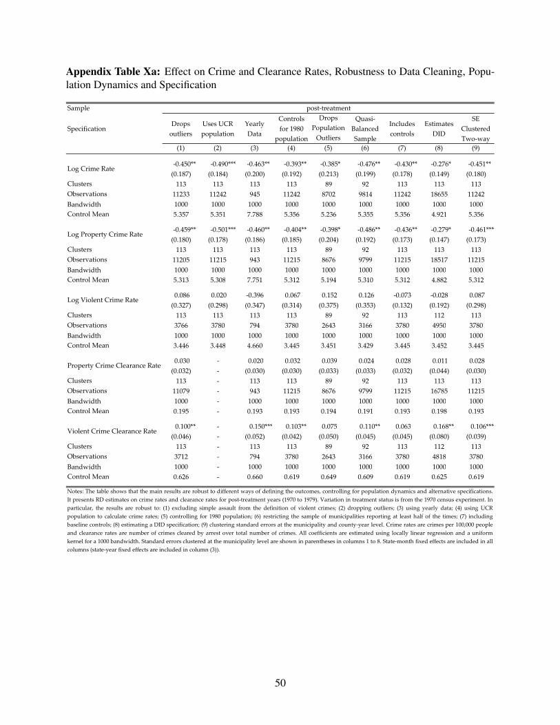
Appendix Table Xa: Effect on Crime and Clearance Rates, Robustness to Data Cleaning, Popu-lation Dynamics and Specification

Sample

SpecificationDrops

outliersUses UCR population

Yearly Data

Controls for 1980

population

Drops Population

Outliers

Quasi-Balanced Sample

Includes controls

Estimates DID

SE Clustered Two-way

(1) (2) (3) (4) (5) (6) (7) (8) (9)

-0.450** -0.490*** -0.463** -0.393** -0.385* -0.476** -0.430** -0.276* -0.451** (0.187) (0.184) (0.200) (0.192) (0.213) (0.199) (0.178) (0.149) (0.180)

Clusters 113 113 113 113 89 92 113 113 113Observations 11233 11242 945 11242 8702 9814 11242 18655 11242Bandwidth 1000 1000 1000 1000 1000 1000 1000 1000 1000Control Mean 5.357 5.351 7.788 5.356 5.236 5.355 5.356 4.921 5.356

-0.459** -0.501*** -0.460** -0.404** -0.398* -0.486** -0.436** -0.279* -0.461*** (0.180) (0.178) (0.186) (0.185) (0.204) (0.192) (0.173) (0.147) (0.173)

Clusters 113 113 113 113 89 92 113 113 113Observations 11205 11215 943 11215 8676 9799 11215 18517 11215Bandwidth 1000 1000 1000 1000 1000 1000 1000 1000 1000Control Mean 5.313 5.308 7.751 5.312 5.194 5.310 5.312 4.882 5.312

0.086 0.020 -0.396 0.067 0.152 0.126 -0.073 -0.028 0.087(0.327) (0.298) (0.347) (0.314) (0.375) (0.353) (0.132) (0.192) (0.298)

Clusters 113 113 113 113 89 92 113 112 113Observations 3766 3780 794 3780 2643 3166 3780 4950 3780Bandwidth 1000 1000 1000 1000 1000 1000 1000 1000 1000Control Mean 3.446 3.448 4.660 3.445 3.451 3.429 3.445 3.452 3.445

0.030 - 0.020 0.032 0.039 0.024 0.028 0.011 0.028(0.032) - (0.030) (0.030) (0.033) (0.033) (0.032) (0.044) (0.030)

Clusters 113 - 113 113 89 92 113 113 113Observations 11079 - 943 11215 8676 9799 11215 16785 11215Bandwidth 1000 - 1000 1000 1000 1000 1000 1000 1000Control Mean 0.195 - 0.193 0.193 0.194 0.191 0.193 0.198 0.193

0.100** - 0.150*** 0.103** 0.075 0.110** 0.063 0.168** 0.106***(0.046) - (0.052) (0.042) (0.050) (0.045) (0.045) (0.080) (0.039)

Clusters 113 - 113 113 89 92 113 112 113Observations 3712 - 794 3780 2643 3166 3780 4818 3780Bandwidth 1000 - 1000 1000 1000 1000 1000 1000 1000Control Mean 0.626 - 0.660 0.619 0.649 0.609 0.619 0.625 0.619

Notes: The table shows that the main results are robust to different ways of defining the outcomes, controlling for population dynamics and alternative specifications.It presents RD estimates on crime rates and clearance rates for post-treatment years (1970 to 1979). Variation in treatment status is from the 1970 census experiment. Inparticular, the results are robust to: (1) excluding simple assault from the definition of violent crimes; (2) dropping outliers; (3) using yearly data; (4) using UCRpopulation to calculate crime rates; (5) controlling for 1980 population; (6) restricting the sample of municipalities reporting at least half of the times; (7) includingbaseline controls; (8) estimating a DID specification; (9) clustering standard errors at the municipality and county-year level. Crime rates are crimes per 100,000 peopleand clearance rates are number of crimes cleared by arrest over total number of crimes. All coefficients are estimated using locally linear regression and a uniformkernel for a 1000 bandwidth. Standard errors clustered at the municipality level are shown in parentheses in columns 1 to 8. State-month fixed effects are included in allcolumns (state-year fixed effects are included in column (3)).

post-treatment

Log Crime Rate

Log Property Crime Rate

Log Violent Crime Rate

Property Crime Clearance Rate

Violent Crime Clearance Rate

50

Appendix Table Xb: Effect on Crime and Clearance Rates, Robustness to OverlappingLegislation

Sample

State being excluded AZ IL IA LA MT NE WI CITY WI VILL(1) (2) (3) (4) (5) (6) (7) (8)

-0.451** -0.443** -0.491** -0.460** -0.459** -0.439** -0.423* -0.466**

(0.187) (0.226) (0.200) (0.191) (0.189) (0.200) (0.221) (0.191)

Clusters 113 60 101 103 108 105 91 110

Observations 11242 5968 9923 10574 10995 10330 8779 10883

Bandwidth 1000 1000 1000 1000 1000 1000 1000 1000

Control Mean 5.356 5.356 5.356 5.356 5.356 5.356 5.356 5.356

-0.461** -0.442** -0.505*** -0.465** -0.467** -0.453** -0.439** -0.476***

(0.180) (0.225) (0.191) (0.182) (0.182) (0.192) (0.214) (0.184)

Clusters 113 60 101 103 108 105 91 110

Observations 11215 5957 9896 10552 10968 10303 8758 10856

Bandwidth 1000 1000 1000 1000 1000 1000 1000 1000

Control Mean 5.312 5.312 5.312 5.312 5.312 5.312 5.312 5.312

0.087 0.027 0.094 0.123 0.082 0.077 0.066 0.087

(0.320) (0.264) (0.335) (0.352) (0.320) (0.326) (0.325) (0.320)

Clusters 113 60 101 103 108 105 91 110

Observations 3780 1338 3409 3376 3742 3543 3506 3766

Bandwidth 1000 1000 1000 1000 1000 1000 1000 1000

Control Mean 3.445 3.445 3.445 3.445 3.445 3.445 3.445 3.445

0.028 0.078 0.028 0.032 0.026 0.016 0.013 0.027

(0.031) (0.057) (0.033) (0.032) (0.031) (0.032) (0.030) (0.032)

Clusters 113 60 101 103 108 105 91 110

Observations 11215 5957 9896 10552 10968 10303 8758 10856

Bandwidth 1000 1000 1000 1000 1000 1000 1000 1000

Control Mean 0.193 0.193 0.193 0.193 0.193 0.193 0.193 0.193

0.106** 0.258*** 0.101** 0.091** 0.103** 0.102** 0.099** 0.105**

(0.042) (0.068) (0.044) (0.044) (0.042) (0.044) (0.044) (0.042)

Clusters 113 60 101 103 108 105 91 110

Observations 3780 1338 3409 3376 3742 3543 3506 3766

Bandwidth 1000 1000 1000 1000 1000 1000 1000 1000

Control Mean 0.619 0.619 0.619 0.619 0.619 0.619 0.619 0.619

Notes: The table shows that the results are not driven by any single state and thus do not depend on other state-specific laws also changing at the same

threshold. The table presents RD estimates on crime and clearance rates for post-treatment years (1970 to 1979), excluding one state at the time. Variation in

treatment status is from the 1970 census experiment. Crime rates are crimes per 100,000 people and clearance rates are number of crimes cleared by arrest over

total number of crimes. Arizona does not have any municipality in the risk set within the specified bandwidth from the threshold. West Virginia is not shown

as there are no municipalities in the risk set within a 3,000 bandwidth from the threshold. The coefficients are estimated using locally linear regression and a

uniform kernel for a 1000 bandwidth. Standard errors clustered at the municipality level are shown in parentheses. State-month fixed effects are included in all

columns.

post-treatment

Log Crime Rate

Log Violent Crime Rate

Property Crime Clearance Rate

Violent Crime Clearance Rate

Log Property Crime Rate

51

Appendix Table Xc: Effect on Crime and Clearance Rates, Robustness to the Estimation

Sample

Estimation

LLR,

Triangular

Kernel

LLR,

Epanech-

nikov

Kernel

LQR,

Uniform

Kernel

LCR,

Uniform

Kernel

LLR,

Uniform

Kernel, no

FEs

LLR,

Uniform

Kernel,

more

flexible

running

variable(1) (2) (3) (4) (5) (6)

-0.550*** -0.541*** -0.632** -0.428 -0.403** -0.452**

(0.207) (0.202) (0.274) (0.291) (0.202) (0.187)

Clusters 113 113 113 113 113 113

Observations 11242 11242 11242 11242 11243 11242

Bandwidth 1000 1000 1000 1000 1000 1000

Control Mean 5.356 5.356 5.356 5.356 5.356 5.356

-0.558*** -0.548*** -0.640** -0.451* -0.422** -0.462**

(0.197) (0.193) (0.259) (0.269) (0.192) (0.180)

Clusters 113 113 113 113 113 113

Observations 11215 11215 11215 11215 11216 11215

Bandwidth 1000 1000 1000 1000 1000 1000

Control Mean 5.312 5.312 5.312 5.312 5.312 5.312

0.108 0.081 0.128 0.342 0.132 0.092

(0.389) (0.364) (0.454) (0.485) (0.268) (0.320)

Clusters 113 113 113 113 113 113

Observations 3780 3780 3780 3780 3941 3780

Bandwidth 1000 1000 1000 1000 1000 1000

Control Mean 3.445 3.445 3.445 3.445 3.445 3.445

0.013 0.016 -0.007 0.008 0.033 0.028

(0.032) (0.032) (0.040) (0.039) (0.034) (0.031)

Clusters 113 113 113 113 113 113

Observations 11215 11215 11215 11215 11216 11215

Bandwidth 1000 1000 1000 1000 1000 1000

Control Mean 0.193 0.193 0.193 0.193 0.193 0.193

0.082* 0.088** 0.067 0.056 0.176*** 0.099**

(0.044) (0.044) (0.057) (0.059) (0.063) (0.042)

Clusters 113 113 113 113 113 113

Observations 3780 3780 3780 3780 3941 3780

Bandwidth 1000 1000 1000 1000 1000 1000

Control Mean 0.619 0.619 0.619 0.619 0.619 0.619

x

Notes: *** p<0.01, ** p<0.05, * p<0.1. The table shows robustness to different choices made in the estimation. It presents RD

estimates on crime and clearance rates for post-treatment years (1970 to 1979). In particular, column 1 and 2 are estimated using

locally linear regression and a triangular kernel and an Epachnikov kernel respectively. They include state-month fixed effects.

Column 3 is estimated using locally quadratic regression and a uniform kernel and includes state-month fixed effects. Column 4

is estimated using locally cubic regression and a uniform kernel and also includes state-month fixed effects. Column 5 is

estimated using locally linear regression and a uniform kernel but does not include state-month fixed effects. Finally, column 6 is

also estimated using locally linear regression and a uniform kernel but allows the running variable to vary by year. Crime rates

are crimes per 100,000 people and clearance rates are number of crimes cleared by arrest over total number of crimes. All

columns present estimates restricting to a 1000 bandwidth. Standard errors clustered at the municipality level are shown in

parentheses.

post-treatment

Violent Crime Clearance Rate

Log Crime Rate

Log Violent Crime Rate

Property Crime Clearance Rate

Log Property Crime Rate

52

Appendix Table XI: Descriptive Statistics for Employment and Expenditures

Statistics N Mean Sd

Employment per 1,000 people 507 26.645 (25.577)

Police Employees per 1,000 people 381 2.681 (1.235)

x

Notes: This table reports summary statistics (number of observations, mean and

standard deviation) for exployment and police employees per 1,000 people for the

baseline sample of post-treatment. Post-treatment years are 1970 to 1979 for

expenditures and 1972 to 1979 for employment.

Appendix Table XII: Descriptive Statistics for Police Officers 1960-1980

Census year 1960 1970 1980 pooled

(1) (2) (3) (4)

Experiment year 1950 1960 1970 1950-1970

Municipalities 132 127 106 365

Police Officers 300 300 250 800

Age 41.350 37.220 34.010 37.730

(12.74) (12.47) (10.41) (12.34)

Highest grade achieved 11.210 13.390 14.940 13.080

(2.416) (2.119) (1.964) (2.663)

Finished high school 0.414 0.712 0.738 0.614

(.493) (.454) (.441) (.487)

Finished two years of college 0.616 0.713 0.455

(.487) (.453) (.498)

Veteran status 0.583 0.434 0.475 0.499

(.494) (.497) (.5) (.5)

x

Panel (a): information on the sample

Panel (b): descriptive statistics

Notes: This table reports descriptive statistics for policemen characteristics. Columns 1 to 3 report

information for a specific census, while column 4 reports information for the pooled sample. The

census year reported at the top of the column refers to when the outcomes are measured; variation

in treatment status is from the census experiment ten year prior. Panel (a) reports the states in the

sample, the number of municipalities, the number of police officers and the number of newly hired

police officers. Panel (b) reports mean and standard deviation for the police officers in

municipalities in the control groups and within a 3000 population bandwidth.

53

Appendix Table XIII: Effect on Demographic Composition of Police Departments, IndividualLevel Regressions

Sample

(1) (2) (3) (4)

-0.088 0.009 -0.002 -0.069

(0.097) (0.093) (0.076) (0.101)

Clusters 136 176 221 134

Observations 400 500 650 400

Bandwidth 750 1000 1250 716

1.362 -1.594 -0.993 -0.892

(2.412) (2.220) (2.054) (2.245)

Clusters 136 176 221 191

Observations 400 500 650 550

Bandwidth 750 1000 1250 1105

-0.019 0.028 0.054 0.036

(0.093) (0.087) (0.074) (0.086)

Clusters 136 176 221 186

Observations 400 500 650 550

Bandwidth 750 1000 1250 1081

Notes: *** p<0.01, ** p<0.05, * p<0.1. The table shows that the effect of merit systems on the

demographic composition of police departments is robust to estimating regressions at the

individual level. It presents RD estimates on a dummy for having a high school degree, age and a

dummy for having veteran status for post-treatment years. Outcomes are measured in the 1960, 1970

and 1980 census, and variation in treatment assignment is from the 1950 to 1970 census. The

coefficients are estimated using locally linear regression and a uniform kernel for four different

bandwidths: 750, 1000, 1250 and an outcome and sample specific MSE-optimal bandwidth. Standard

errors clustered at the municipality level are shown in parentheses. State-census year fixed effects

are included in all columns. Observation numbers are rounded to avoid disclosure.

post-treatment

Finished High School

Age

Veteran

Appendix Table XIV: Effect of Merit Systems on Turnover and Wages

Sample

(1) (2) (3) (4)

-0.000 0.098 0.088 -

(0.127) (0.123) (0.109) -

Clusters 119 159 191 -

Observations 99 129 155 -

Bandwidth 750 1000 1250 -

0.395 0.628 0.651 0.579

(0.636) (0.529) (0.463) (0.608)

Clusters 179 236 302 197

Observations 136 176 221 149

Bandwidth 750 1000 1250 823

x

x

Notes: *** p<0.01, ** p<0.05, * p<0.1. The tables shows the effect of the merit system mandate on

outcomes related to the organization of police departments. The table presents RD estimates on

turnover and wages for post-treatment years. The outcomes are fraction of police officers who are

certaintly new hires and average wage. Outcomes are measured in the 1960, 1970 and 1980 census,

and variation in treatment assignment is from the 1950 to 1970 census. The coefficients are

estimated using locally linear regression and a uniform kernel for four different bandwidths: 750,

1000, 1250 and an outcome and sample specific MSE-optimal bandwidth. Standard errors clustered

at the municipality level are shown in parentheses. State-census year fixed effects are included in all

columns.

post-treatment

Average Wage

Fraction New Hire

54

Appendix Table XV: Heterogeneous Effects by Whether Chief under Merit System

Sample

(1) (2) (3) (4)

-0.480** -0.363* -0.303* -0.535**

(0.238) (0.201) (0.175) (0.246)

-0.817*** -0.640*** -0.584*** -0.883***

(0.228) (0.208) (0.191) (0.239)

Clusters 89 113 137 76

Observations 8906 11242 13623 7730

Bandwidth 750 1000 1250 661

Control Mean 5.410 5.356 5.313 5.453

Pvalue 0.127 0.150 0.112 0.123

post-treatment

Log Crime Rate*Chief Not Protected

Log Crime Rate*Chief Protected

Notes: *** p<0.01, ** p<0.05, * p<0.1. The table shows that heterogeneous effects by whether the police

chief was also covered by a merit system. The table presents RD estimates on crime rates interacted with

a dummy for being in a state whether the chief was or was not covered for post-treatment years (1970 to

1979). Variation in treatment status is from the 1970 census experiment. The coefficients are estimated

using locally linear regression and a uniform kernel for four different bandwidths: 750, 1000, 1250 and

an outcome and sample specific MSE-optimal bandwidth. Standard errors clustered at the municipality

level are shown in parentheses. The p-value reported is from a test of equality of the two coefficients.

State-month fixed effects are included in all columns.

Appendix Table XVI: Effect of Merit System Mandates on Reporting post-1980

Sample(1) (2) (3) (4)

0.005 0.041 0.056 0.060(0.053) (0.059) (0.053) (0.053)

Clusters 74 103 130 49Observations 8880 12360 15600 5880Bandwidth 750 1000 1250 553Control Mean 0.070 0.071 0.101 0.073

x

post-treatment

Monthly Crime Report Missing

Notes: *** p<0.01, ** p<0.05, * p<0.1. The table shows that police departments did not differentiallyreport crime data to the police in the 1980 census experiment. It presents RD estimates of the effectof merit systems on a dummy equal to one if the department did not submit a report for the monthfor post-treatment years (1980 to 1989, columns 1 to 4). Variation in treatment status is from the1980 census experiment. The coefficients are estimated using locally linear regression and a uniformkernel for four different bandwidths: 750, 1000, 1250 and an outcome and sample specific MSE-optimal bandwidth. Standard errors clustered at the municipality level are shown in parentheses.State-month fixed effects are included in all columns.

55