Civil Service and Patronage in Bureaucracies∗

John D. Huber

Department of Political Science

Columbia University

Michael M. Ting

Department of Political Science and SIPA

Columbia University

October 9, 2016

Abstract

We develop a model of government personnel policy with electoral competition in aneffort to understand when high quality bureaucracies will be created and sustained.In the model, two parties compete for office over an infinite horizon, and politiciansin office choose a mix between civil servants (who produce public goods in a goodbureaucracy) and patronage appointees (who produce private goods and can influencere-election). Civil servants make future good bureaucracies more likely, and thus per-sonnel policies depend on incumbents’ electoral prospects and the anticipated actionsof future politicians. Civil service hiring is maximized when both parties value pub-lic goods. It is also affected by the electoral vulnerability of the incumbent, but thedirection of this relationship depends on characteristics of the opposition, calling intoquestion previous arguments about electoral vulnerability and civil service reforms.Numeric results on long-run behavior suggest that electorally dominant parties canincrease long-term bureaucratic quality, electorally weak parties are associated withhigher bureaucratic quality, and that polarization reduces bureaucratic quality andamplifies partisan advantages. Finally, we present empirical evidence regarding a coreimplication of our model about the relationship between party preferences and meri-tocratic civil service hiring.

∗We thank Anna Bassi, Katherine Bersch, Scott Desposato, Francisco Garfias, Samuel Kernell, MalteLierl, Carlo Prato, Christian Schuster, Tara Slough, conference participants at the 2015 APSA, 2016 EmoryCSLPE, and 2016 EPSA meetings, and seminar participants at Columbia, UCSD, Stanford, Yale, Vanderbilt,and the Inter-American Development Bank for helpful comments.

1 Introduction

Good governance requires good bureaucracy, where civil servants do the day-to-day work

delivering the public goods that government can best provide. But in democracies, politicians

who worry about re-election and the policy consequences of losing may lack incentives to

create good bureaucracy. Incumbents may instead prefer patronage-based systems that

encourage bureaucrats to work on behalf of electoral or other political goals. Such activities

undermine professionalism and make it more difficult to achieve good governance.

This paper develops a theory to study this trade-off. Its central purpose is to understand

the electoral, ideological, and social factors that affect the creation of good bureaucracies.

At the heart of the model is the premise that personnel systems determine bureaucratic

production. On one hand, professional civil servants can produce public goods like defense,

property rights enforcement, contract enforcement, education, internal security and public

infrastructure that benefit the vast majority of citizens, regardless of who controls public

office (e.g., Rauch 1995, Rauch and Evans 2000, Krause, Lewis and Douglas 2006, Lewis

2008, Gerber and Gibson 2009). Professional civil servants are largely insulated from political

pressure, with policies in place – and respected – that ensure job security and merit-based

hiring and promotion.

On the other hand, patronage appointees produce private goods that specifically benefit

the party in power. Such private goods can include policies that benefit the party elite,

policies that benefit party supporters, and campaign activities that help the party get re-

elected (e.g., Pollock 1937, Reid and Kurth 1989, Folke, Hirano and Snyder 2011). Election

winners can hire and fire patronage appointees at will, and patronage jobs are at once

rewards for helping a party win an election and incentives to help that party win re-election.

Patronage-based bureaucrats typically lack the skills, experience and especially the incentives

to produce public goods. Even in advanced countries, most bureaucracies mix civil servants

and patronage appointees, and the goal of the model is to understand how democratic

1

competition generates the distribution of personnel and its attendant governance outcomes.

Several features of bureaucracy and political competition are central to our model. First,

investing in civil service reform does not automatically produce good governance. In the U.S.,

for example, federal civil service reform began with the 1883 Pendelton Act, which required

merit-based selection of civil servants. But civil servants were not protected from dismissal

until the 1912 Lloyd-La Follette Act, and were not restricted from political activities until

the 1939 Hatch Act. In addition, the histories of civil service reform in numerous U.S. states

show that legislated reforms can be reversed by future political actions. Reforms that persist

can also be weakened. In Latin America, most countries have adopted civil service reforms

in recent decades but have adopted a range of strategies to circumvent them (Grindle 2012).

This observation implies that the factors that contribute to the existence of high quality

bureaucracies – e.g., insulation from political pressure, merit based-hiring and promotion,

and competitive salaries – take time to take effect. Thus, investments in the civil service

require some anticipated future benefit. Low-quality, patronage-based bureaucracies do not

have this feature. Indeed, they are valuable precisely because the incumbent expects a

short-term benefit of putting “its own people” in public positions. We therefore consider a

dynamic model, where incumbent politicians must anticipate not only how personnel policies

affect their current policy choices and electoral prospects, but also how the opposition will

approach these issues if it wins the election.

Second, incumbents cannot exploit a good bureaucracy for electoral gain. Voters thus

know that civil servants will produce public goods no matter which party is in control,

decreasing the salience of bureaucracy to vote choice. Civil service rules also prevent all

bureaucrats from knocking on doors at election time, or from engaging in other activities for

the benefit of incumbents. By contrast, under a low quality bureaucracy, parties can exploit

patronage appointees for electoral gain. Thus, politicians care about government personnel

not only because they affect policy outcomes, but also because they can affect elections. The

model therefore incorporates differential electoral implications of bureaucratic quality.

2

Third, parties differ in their induced preferences for high quality bureaucracy. These

preferences may be linked to policy. A class-based party, for example, may value public goods

like tax enforcement because such enforcement facilitates redistribution. The preferences

might also be linked to electoral considerations. An ethnic-based party, for example, may

rely on patronage appointments to encourage ethnic political competition. And parties in

the same political system may differ in their ability to attract civil servants. This may

be a particular issue following transitions from authoritarian rule to democracy, especially

if there has been a history of ethnic or racial politics. Following the second Iraq war, for

example, the Shia-dominated party that won the first election faced a bureaucracy loyal to the

Sunni-dominated government under Saddam Hussein, and most individuals with experience

running the state were Sunnis. Even if there had been formal civil service procedures in

place, it would have been more challenging for the inexperienced Shia party to hire qualified

individuals to produce public goods, which in turn could have increased that party’s emphasis

on patronage. A similar situation likely existed in South Africa following the fall of apartheid,

and in some British colonies following independence. The model therefore allows differences

in the parties’ preferences for public goods and their costs of hiring civil servants.

These features undergird our model of bureaucratic structure. In the model, two parties

compete for power over an infinite horizon. Each party is led by a candidate who can serve

in government for up to two periods. The winning candidate chooses the mix of civil servants

and patronage appointees. Civil servants contribute to the production of public goods if the

bureaucracy is high quality, and also increase the likelihood of a high quality bureaucracy

in the subsequent period. Patronage appointments produce private goods in the current

period regardless of bureaucratic quality. Each party has an exogenous base probability of

winning each election, but under a low quality bureaucracy patronage appointments improve

the incumbent party’s electoral prospects.

We derive a unique Markov perfect equilibrium of the game, which allows us to address

three types of questions about bureaucratic structure. First, following any given election,

3

what affects the incentives of the winning candidate to invest in the civil service rather

than patronage? Second, over the long-run, under what conditions should we expect good

governance to prevail? And third, how do politicians’ incentives with respect to bureaucratic

structure influence electoral competition?

To see the intuition of the equilibrium, consider the situation of a newly elected politician

who inherits a low quality bureaucracy. The incentive to hire civil servants is affected not

only by the politician’s preferences and costs, but also by characteristics of the opposition.

This is because investments in civil service take time to bear fruit, and can effect public

goods production only in the subsequent period. Additionally, if the politician is not re-

elected, the public goods that will be produced in the subsequent period will increase as

the opposition has greater incentives to produce public goods. Thus, a politician will hire

more civil servants when there are dynamic complementarities; i.e., if the opposition places

a high value on public goods and has low costs of civil service hiring. These features of the

opposition matter more when the incumbent is electorally vulnerable.

This observation highlights a considerable challenge of creating a high quality bureaucracy

where none exists. A collective action problem of sorts emerges from the fact that the party

that initially invests in good government bears a cost (forgoing the electoral benefits of

patronage while reaping no public goods) that the other party does not. Thus, each party

prefers that the other make the initial investment. To overcome this problem, it is not

enough for the incumbent party to have characteristics that foster good governance. If there

are competitive elections, it is crucial that the opposition has these characteristics as well.

Our theory unifies two common but conflicting accounts linking incumbent electoral

vulnerability and with political reforms such as civil service systems. One view is that in-

cumbents will undertake reform when they are electorally vulnerable in order to constrain or

induce particular policy choices of future politicians (Moe 1989, Geddes 1994, de Figueiredo

2002, Ruhil and Camoes 2003, Lewis 2008, Besley and Persson 2011, Ting, Folke, Hirano,

and Snyder 2013, Lavertu 2013, Mueller 2015). The opposite argument is that incumbents

4

undertake reform when they are electorally secure. This perspective treats reforms as an

“investment,” and politicians need the assurance of remaining in power in order to reap the

benefits of reform (Besley and Persson 2010, Acemoglu, Ticchi, and Vindigni 2011). Our

results suggest that the direction of the relationship depends on the characteristics of the

opposition. When the opposition favors private goods, the incumbent has less to gain from a

good bureaucracy and more to gain from patronage appointees who can help win re-election.

In this situation, the investment logic prevails and civil service hires should decrease with

electoral vulnerability. That is, reform is useful in this situation because the incumbent can

expect the opposition party to to produce public goods if it wins.

We exploit the Markov structure of the equilibrium to arrive at numerical results on

the persistence of bureaucratic quality and the long-run probabilities of a high quality bu-

reaucracy. This analysis suggests that electoral competition – where no party has a large

electoral advantage – will maximize bureaucratic quality only under quite limited condi-

tions. In particular, there need to be even costs of civil service hiring across parties, and low

party system polarization. Otherwise, long-run bureaucratic quality is maximized when the

electorally advantaged party also has low costs. Yet interestingly, the opposition party is

able to reap the benefits of this investment, as the electorally disadvantaged party will more

frequently govern with a good bureaucracy.

Our numerical results also demonstrate that polarization creates a consequential electoral

role for the bureaucracy. When party system polarization is high, personnel strategies help

to entrench the electoral security of the favored party, particularly when the favored party

has higher costs of hiring civil servants. When polarization is low, personnel strategies have a

much weaker relationship with electoral outcomes. Thus, the model suggests that patronage-

based systems persist in countries where there is high polarization across parties or groups

and electorally advantaged parties do not have a cost advantage in civil service hiring.

In addition to developing the theoretical model, we use cross-national data to provide

two types of empirical evidence relevant to out model. First we show that countries that are

5

most meritocratic in their civil service hiring practices also have the highest levels of good

government. Second, we examine the link between party preferences and civil service hiring

by assuming that a reasonable proxy for whether parties are oriented more towards providing

public or private goods is the degree to which parties receive support from specific ethnic

groups. When parties tend to receive support from different ethnic groups, they should have

weaker incentives to produce public goods that benefit all citizens equally. Our cross-national

data show that ethnic diversity itself is unrelated to lower levels of meritocratic hiring but

the ethnification of parties is associated with lower levels of such hiring.

The paper proceeds as follows. Section 2 describes the model and section 3 describes

the equilibrium. Sections 4 and 5 analyzes comparative statics, with section 4 focusing on

incentives politicians have to invest in civil service and section 5 focusing on the on long-run

numerical results about bureaucratic quality and electoral impacts. Section 6 provides our

empirical results and section 7 concludes.

1.1 Related Literature

Our model joins an emerging body of theoretical work on the relationship between elections

and bureaucrats. The distinction between the production of political appointees and civil

servants resembles that of Rauch’s (1995) study of U.S. municipal governments. More recent

models that incorporate electoral concerns include Ujhelyi (2014) and Nath (2015). All of

these papers focus on the incentives of bureaucrats, while we focus on the long-run behavior

of politicians and leave bureaucratic behavior non-strategic. One exception that explores

politician’s personnel policy choices over an infinite horizon is Ting, Folke, Hirano, and

Snyder (2013), who consider a simpler environment with non-reversible civil service reforms.

A closely related and now extensive literature explores the origins of civil service re-

form (Knott and Miller 1987, Johnson and Libecap 1994, Horn 1995, Gailmard and Patty

2007, Hollyer 2011). Elections typically play a prominent role in these accounts, and the

6

lock-in arguments described previously have also featured prominently in arguments about

judicial independence (e.g., Ramseyer 1994, Stephenson 2003) and state politicization (e.g.,

Grzymala-Busse 2003). Some of the non-electoral factors emphasized include interest group

politics, economic development, expertise, and the costs of patronage systems.

A number of recent papers have explored the political determinants of dynamic public

goods provision (e.g., Azzimonti 2011). Our emphasis on its institutional foundations relates

to a growing scholarly interest in “state capacity” (Huber and McCarty 2004, Ting 2011),

which has sometimes been interpreted as the ability to collect taxes (Besley and Persson

2010). The theoretical approach most closely related to ours is Acemoglu, Ticchi, and

Vindigni (2011), who develop a theory of redistribution and state efficiency with an infinite

horizon model that features electoral competition and endogenous taxes, pork, bureaucratic

quality, and bureaucratic size. Their paper shares our assumptions about the constraints

of bureaucratic quality on policy and the effect of personnel choices on future quality, but

it focuses on emerging democracies and how the rich can use inefficient personnel policy to

affect redistribution, particularly when inequality is high.

Finally, the model serves as a potential basis for theoretically informed empirical research

on government personnel systems and the quality of government. Numerous authors have

documented the effects of public sector employment on electoral outcomes in the U.S. (e.g.,

Folke, Hirano and Snyder (2011) and elsewhere (e.g., Roett 1999, Golden 2003). In our view,

a logical next step would be to address directly the relationships between personnel policies

and measures of the quality of governance (Knack and Keefer 1995, La Porta, Lopez-de-

Silanes, Shleifer, and Vishny 1999, Rauch and Evans 2000).

2 Model

The model features partisan elections and personnel decisions over an infinite horizon. There

are two political parties, A and B, each of which produce a sequence of identical candidates,

7

with one drawn each period. A newly elected candidate may hold office for up to two periods,

and cares about retaining office and policies over both periods of political life regardless of

whether she is re-elected. The politician in office determines the distribution of government

personnel, which affects the quality of the bureaucracy, the production of public and private

goods, and the probability that the incumbent can be re-elected. There is no discounting. If

a sitting incumbent is in her first term, she becomes her party’s candidate in the subsequent

election. Otherwise, the party draws a new candidate.

The bureaucracy is composed of a unit measure of non-strategic bureaucrats, who can

be of two types: civil servants can produce public goods that benefit both parties, while

patronage appointees can produce private goods that benefit only the incumbent party.

Patronage appointees can also directly enhance the incumbent party’s chance of re-election

(see below). In each period, t, the a party i politician chooses the proportion of civil servants

cti ∈ [0, 1]. The remaining 1− cti bureaucrats are patronage appointees.

The composition of the bureaucracy affects its quality, denoted by qt ∈ 0, 1. A bad bu-

reaucracy (qt = 0) can produce private but not public goods. A good bureaucracy (qt = 1)

has the combination of professionalism, talent and insulation from political pressure nec-

essary to produce public goods. Importantly, incumbents cannot instantly establish good

bureaucracies; civil service rules and procedures take time to develop and take hold. Thus,

bureaucratic quality is determined by personnel choices in the previous period. If party i

was in power in period t − 1, then the bureaucracy is good in period t with probability

Prqt = 1 | ct−1i = ct−1

i and bad with probability Prqt = 0 | ct−1i = 1 − ct−1

i . Thus, the

probability of a good bureaucracy in period t is increasing in the previous period’s level of

civil servants, and is also independent of quality in preceding periods.

Public goods production under a good bureaucracy in period t with a party i incumbent

is given by cti. Private goods production does not depend on bureaucratic quality, and is

given by 1− cti. Politicians can therefore exploit a good bureaucracy by hiring civil servants,

and in so doing, they increase the probability of a good bureaucracy in the future. Incentives

8

to produce public and private goods can vary across parties. Let wi ∈ [0, 1] denote party

i’s marginal valuation of public goods, and let 1 − wi be its marginal valuation of its own

private goods. Party i’s valuation of party j 6= i’s private goods is 0. The parameter wi is

an inverse measure of party i’s policy extremism: as wi increases, i becomes more interested

in the mutually beneficial policy. Thus, we say that party system polarization increases as

wA and wB both decrease.

Politicians face two kinds of costs. First, each incumbent politician incurs a fixed cost k ∈

[0, 1] for losing her re-election bid.1 This assumption assures that no politician can be better

off from losing than from winning, and can be considered a simple form of office motivation.

Second, the relative costs of hiring civil servants as opposed to patronage appointees can

vary within and across parties. The cost to a party i politician of cti civil servants is βi(cti)

2,

and the cost of the remaining 1− cti patronage appointees is αi(1− cti)2, where αi = 2 − βi

and βi ∈ (12, 3

2).

A party i politician’s utility from bureaucratic appointments in period t can therefore be

written as follows:

ui(ct, qt) =

qtwicti + (1−wi)(1−cti)−βi(cti)2−αi(1−cti)2 if party i is in power

qtwictj if party j 6= i is in power.

(1)

Bureaucratic appointments can influence election outcomes. Each party i has a base

re-election probability of γi ∈ (0, 1), where γA = 1 − γB. When the bureaucracy is good,

patronage appointments do not affect election prospects because the civil service system

ensures that even patronage appointees cannot undertake activities that benefit the incum-

bent’s electoral prospects. When the bureaucracy is bad, patronage appointees improve the

incumbent party’s election prospects. Thus, if i is an incumbent eligible for re-election at

1We bound k so that its magnitude can be no greater than the maximal policy benefit in a given period.

9

time t, her re-election probability is given by:

ρi(cti, q

t) = γi + (1− qt)mi(1− cti), (2)

where mi ∈ (0, 1−γi) measures the effectiveness of patronage appointees at delivering votes.

The opposition party wins the election with probability 1−ρi(qt). In what follows, we assume

that m = mA = mB, though this assumption is not necessary for the results.

The model captures a number of incentives in the choice of a personnel system. Profes-

sional civil servants can provide public goods when the bureaucracy is good, and also improve

the chances that a good bureaucracy will be sustained in the future. First term incumbents

may then invest in civil servants not only to produce public goods if they are re-elected, but

also to benefit from public goods if they lose their re-election bids. By contrast, patronage

appointees produce private goods for the incumbent, and can be used to maintain power

when the bureaucracy is bad. A newly-elected politician therefore faces different trade-offs

depending on inherited bureaucratic quality, but must always consider the future ability to

produce public goods.

We derive a unique Markov Perfect equilibrium, and therefore dispense with notation for

time periods in what follows. The state variables are given by the triple (i, n, q), where

i ∈ A,B is the party in power, n ∈ 1, 2 is the term of the current incumbent, and

q ∈ 0, 1 is bureaucratic quality. Denoting the set of states by S, each party’s strategy

is a mapping S → [0, 1] from the state space to a level of civil service appointments. For

convenience, we denote the civil service appointments by a party i politician in her n-th term

of office under bureaucratic quality q by cnqi , so for example civil service hiring by a newly

elected Party A politician who inherits a bad bureaucracy is c10A .

Using this notation, the expected utility of a newly-elected (first-term) party i incumbent

as a function of her level of civil service appointments c and bureaucratic quality q can be

10

written as follows:

EUi(c|s) = ui(c, q) + ρi(c, q)[cui(c

21i , 1) + (1− c)ui(c20

i , 0)]

+

(1− ρi(c, q))[cui(c

11j , 1) + (1− c)ui(c10

j , 0)− k]. (3)

The first term is the utility in the current period (as described in equation (1)) from the

public and private goods that are produced as a function of c, as well as the cost of her

personnel appointments. The second term in equation (3) is the probability of re-election

ρi(·) and her payoff conditional upon re-election, and the third term analogously expresses

the case where party j 6= i wins the election and sets future personnel policy. In both cases,

bureaucracy quality is good in the subsequent period with probability c. Thus the choice of

c affects i’s expected utility through immediate bureaucratic production, its possible effect

on re-election, and future bureaucratic quality.

3 Equilibrium

We begin by solving for c2qi , or the personnel choices of second term party i politicians. A

second term politician simply chooses the level of civil service that maximizes her utility

according to (1). The stage utility function is concave for all c ∈ [0, 1] with a second

derivative of −4, and thus i’s optimal level of civil service hires is:

c2qi =

3 + wi(1 + q)− 2βi4

. (4)

This expression is obviously interior for all q.

When choosing the level of civil servants in the first period, the politician anticipates

that she will adopt c2qi if re-elected. She further anticipates how her choice will affect not

only her probability of re-election, but also what a party j politician would choose. To this

11

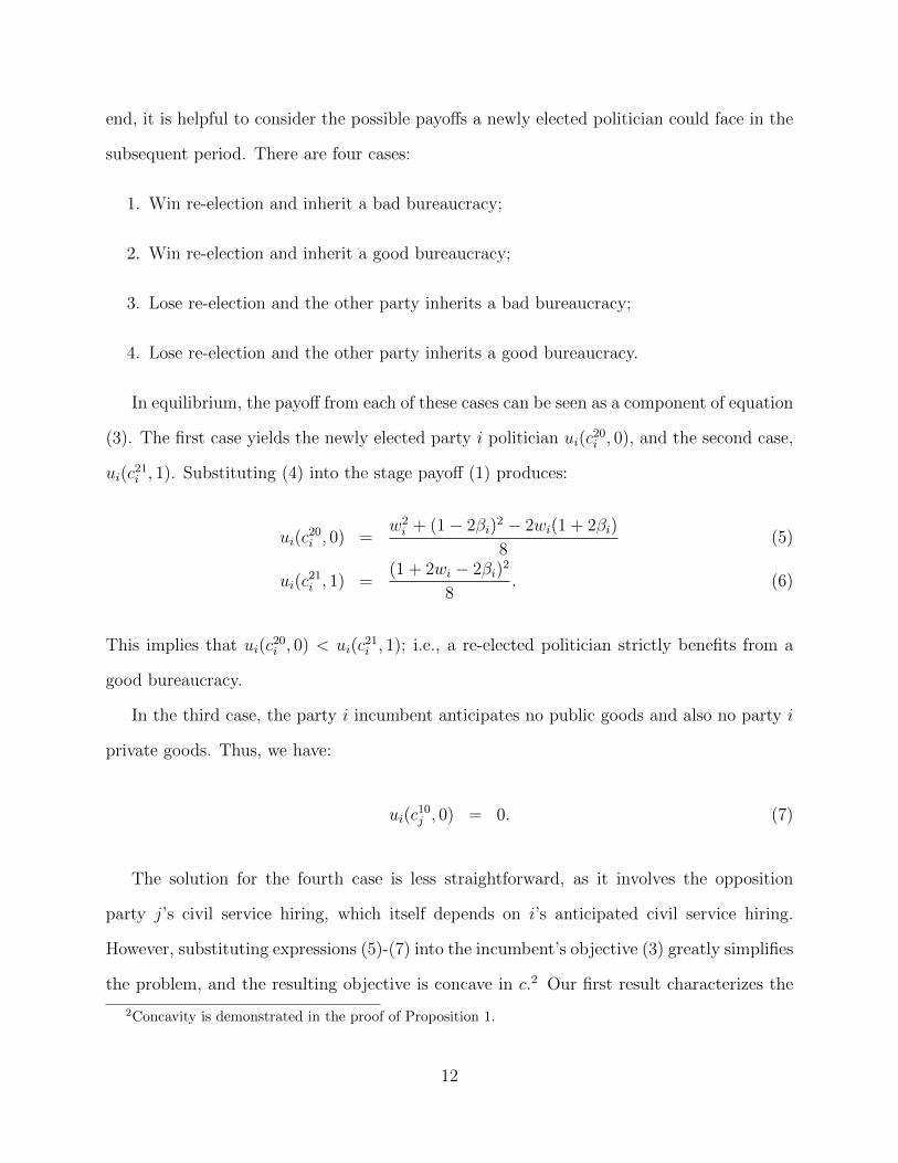
end, it is helpful to consider the possible payoffs a newly elected politician could face in the

subsequent period. There are four cases:

1. Win re-election and inherit a bad bureaucracy;

2. Win re-election and inherit a good bureaucracy;

3. Lose re-election and the other party inherits a bad bureaucracy;

4. Lose re-election and the other party inherits a good bureaucracy.

In equilibrium, the payoff from each of these cases can be seen as a component of equation

(3). The first case yields the newly elected party i politician ui(c20i , 0), and the second case,

ui(c21i , 1). Substituting (4) into the stage payoff (1) produces:

ui(c20i , 0) =

w2i + (1− 2βi)

2 − 2wi(1 + 2βi)

8(5)

ui(c21i , 1) =

(1 + 2wi − 2βi)2

8. (6)

This implies that ui(c20i , 0) < ui(c

21i , 1); i.e., a re-elected politician strictly benefits from a

good bureaucracy.

In the third case, the party i incumbent anticipates no public goods and also no party i

private goods. Thus, we have:

ui(c10j , 0) = 0. (7)

The solution for the fourth case is less straightforward, as it involves the opposition

party j’s civil service hiring, which itself depends on i’s anticipated civil service hiring.

However, substituting expressions (5)-(7) into the incumbent’s objective (3) greatly simplifies

the problem, and the resulting objective is concave in c.2 Our first result characterizes the

2Concavity is demonstrated in the proof of Proposition 1.

12

unique equilibrium level of civil servants chosen by new politicians. The result is stated in

terms of Ωi = ui(c11j , 1), which is a party i first-term incumbent’s stage game payoff when

she is not re-elected and the bureaucracy is good. All proofs are found in the Appendix.

Proposition 1 Civil Servants for First Term Politicians. In the unique Markov perfect

equilibrium, the interior solution is

c10i =

1

2+

3w2i γi −m(8k + w2

i + (1− 2βi)2 − 2wi(1 + 2βi))+

wi(8 + (6− 4βi)γi) + 8(1− 2βi + (1− γi)Ωi)

32 + 2m(3w2i + wi(6− 4βi)− 8Ωi)

, (8)

c11i =

1

2+

3w2i γi + wi(16 + (6− 4βi)γi) + 8(1− 2βi + (1− γi)Ωi)

32, (9)

where

Ωi =

wi(96− 64βj + 12w2j (1− γi) + wj(88− 16βj(1− γi)−

16βiγi + 3w2i γ

2i + 2wiγi(8 + 3γi − 2βiγi)))

8(16− wiwj(1− γi)γi).

Along with expression (4), Proposition 1 characterizes the unique interior equilibrium

personnel strategies. We focus on the interior solutions for the remainder of the paper, and

note that corner solutions for the personnel choices of newly elected politicians exist only for

some extreme parameter values.

Comparing policy choices across periods provides a first glimpse at the roles of bureau-

cratic quality and electoral concerns. It is easily verified that c11i > c21

i , as the maintenance

of a good bureaucracy strictly increases a new politician’s incentive to hire civil servants. By

contrast, the relationship between c10i and c20

i is ambiguous. This is because a new politician

additionally takes her election prospects into account when choosing c under a low quality

bureaucracy.

The comparative statics on personnel strategies with respect to the incumbent party’s

cost and preference parameters are straightforward to derive and summarized in the fol-

lowing comment. Regardless of bureaucratic quality, civil service hiring is increasing in the

13

incumbent’s valuation of public goods and decreasing in its cost of hiring civil servants. Ad-

ditionally, it can be shown that civil service hiring is decreasing in m when k is high enough

for politicians to want re-election. As the next sections will show, the results for electoral

advantage and characteristics of the opposition party are somewhat less intuitive.

Comment 1 Basic Comparative Statics. When a first term party i politician inherits a

bureaucracy of quality q,

∂c1qi

∂wi> 0 and

∂c1qi

∂βi< 0.

4 Investing in Good Government

What factors influence the creation of good bureaucracy where none exists? Suppose that

party A’s candidate has won the election and must decide how much to invest in civil

service (i.e., c10A ) and patronage, and that party B is in opposition, and will thus make

its own personnel choice if A loses. We consider three factors that affect A’s investment:

characteristics of the opposition, party system polarization, and the electoral environment.

4.1 Opposition Characteristics

When A inherits a bad bureaucracy, the value of investing in civil service lies strictly in the

future because civil servants cannot produce public goods in the current period. If A wins

re-election, she will adopt her optimal level of civil service according to equation (4), which

is independent of any characteristic of B. But if A loses re-election, she receives a payoff in

the next period only if B produces public goods, which can only occur if A’s investment in

civil service produces a good bureaucracy. A’s payoff from hiring civil servants is therefore

affected by characteristics of B that affect B’s incentives to hire civil servants if B inherits

a good bureaucracy.

14

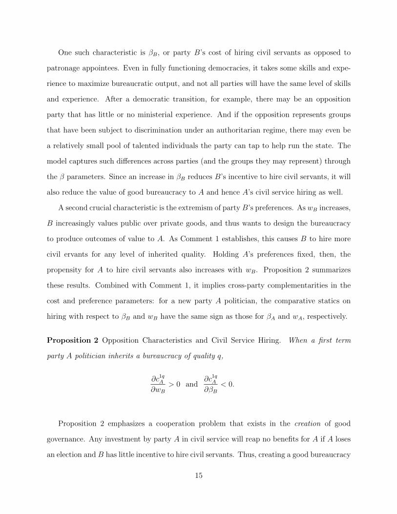
One such characteristic is βB, or party B’s cost of hiring civil servants as opposed to

patronage appointees. Even in fully functioning democracies, it takes some skills and expe-

rience to maximize bureaucratic output, and not all parties will have the same level of skills

and experience. After a democratic transition, for example, there may be an opposition

party that has little or no ministerial experience. And if the opposition represents groups

that have been subject to discrimination under an authoritarian regime, there may even be

a relatively small pool of talented individuals the party can tap to help run the state. The

model captures such differences across parties (and the groups they may represent) through

the β parameters. Since an increase in βB reduces B’s incentive to hire civil servants, it will

also reduce the value of good bureaucracy to A and hence A’s civil service hiring as well.

A second crucial characteristic is the extremism of party B’s preferences. As wB increases,

B increasingly values public over private goods, and thus wants to design the bureaucracy

to produce outcomes of value to A. As Comment 1 establishes, this causes B to hire more

civil ervants for any level of inherited quality. Holding A’s preferences fixed, then, the

propensity for A to hire civil servants also increases with wB. Proposition 2 summarizes

these results. Combined with Comment 1, it implies cross-party complementarities in the

cost and preference parameters: for a new party A politician, the comparative statics on

hiring with respect to βB and wB have the same sign as those for βA and wA, respectively.

Proposition 2 Opposition Characteristics and Civil Service Hiring. When a first term

party A politician inherits a bureaucracy of quality q,

∂c1qA

∂wB> 0 and

∂c1qA

∂βB< 0.

Proposition 2 emphasizes a cooperation problem that exists in the creation of good

governance. Any investment by party A in civil service will reap no benefits for A if A loses

an election and B has little incentive to hire civil servants. Thus, creating a good bureaucracy

15

requires cooperation across parties. The prospect of such cooperation will diminish when the

other party has relatively high costs of civil service or relatively extreme preferences. Even

when A inherits a good bureaucracy, incentives to invest in civil service will diminish when

B has extreme preferences or high civil service hiring costs.

4.2 Party System Polarization

Another measure of party systems of interest is party system polarization, which is a situ-

ation where both A and B want to produce private goods. We can capture the inverse of

polarization in a single parameter by assuming w = wA = wB. Proposition 3 shows that

investment in civil service is decreasing in party system polarization, regardless of whether

A inherits a good or bad bureaucracy. The result follows directly from the application of

Comment 1 and Proposition 2.

Proposition 3 Party System Polarization. Let w = wA = wB. Then:

∂c10A

∂w> 0 and

∂c11A

∂w> 0.

Polarized party systems, then, are bad for good government in a competitive democracy.

When both parties use the bureaucracy for electoral gain and private goods production, they

will be unable to “cooperate” by sustaining consistently high civil service hiring. Thus, the

model suggests that electoral systems and social structures that encourage centripetal rather

than centrifugal party competition will help in the creation of good bureaucracy.

4.3 Electoral Context

Next consider the electoral context. As noted in the introduction, scholars have emphasized

that politicians may wish to invest in the civil service when they are electorally vulnerable

16

as a way to improve outcomes if they fall out of power. The typical mechanism in these

arguments is some form of lock-in. If an incumbent party expects to lose an election, the

argument goes, rigid civil service procedures can make it difficult for the electoral foe to

change policy, or to divert the bureaucracy’s actions to its own private ends. Civil service,

then, emerges from conflict and distrust between parties.

The model here departs from this lock-in logic in one important respects. The first

concerns the mechanism by which an incumbent faced with electoral loss might benefit from

hiring civil servants. When the bureaucracy is bad, an investment in the civil service can

reap only a future benefit. And the future benefit will be realized only if the opposition

hires civil servants after winning. The opposition cannot be forced to do so; that is, its

hands cannot be tied. Thus, rather than tying the hands of the other party, the incumbent

invests in civil service to encourage the opposition party to also invest in civil service, and

thus to produce public goods. This perspective suggests that good bureaucracy requires –

and emerges from – synergistic commitments to civil service that exist across parties, rather

than from conflict and distrust between them.

A key feature of our model is that decisions about bureaucratic structure can affect elec-

toral outcomes. Since vulnerable incumbents can choose personnel structures that increase

their chances of re-election, and hiring civil servants carries an electoral cost, investment in

civil service need not increase with electoral vulnerability, as the lock-in logic argues. The

model predicts that both positive and negative relationships between electoral vulnerabil-

ity and civil service investment are possible, and the direction of the effect depends on the

expected benefits to the incumbent of creating good government for the opposition.

As an example, if the opposition’s preferences are relatively moderate (so that wB is

relatively high), as A becomes more electorally insecure, she benefits in the future from a

good bureaucracy because so doing will give B an incentive to appoint civil servants. This

situation therefore results in a relationship that is consistent (in direction) with that of lock-

in arguments: the more electorally insecure the incumbent, the more the incumbent invests

17

in civil service. However, as B’s preferences become more extreme, A has less to gain from

investing in civil service (because the future production of public goods when B wins will

be lower). This weakens the relationship between γA and civil service investment. Figure 1

depicts how the equilibrium level of civil servants changes with γA at different values of wB.

If B’s preferences become sufficiently extreme (i.e., wB sufficiently low), the direction

of the effect of γA on civil service investment can change. The future value to A of a

good bureaucracy under B is low if B has little desire for public goods. This increases A’s

incentives to get re-elected and encourages the hiring of patronage appointees. But as A’s

electoral security increases, she will have an increasing incentive to appoint civil servants in

order to take advantage of the public goods they may produce upon re-election. Thus, we

have the opposite of the lock-in argument: the optimal level of civil servants is increasing

in γA at sufficiently low wB. We can see this in Figure 1, where civil service investment is

increasing in γA when wB is low.

By an identical logic, the direction and magnitude of the effect of γA on hiring varies

with civil service personnel costs βB. A high value of βB plays a similar role to a low value of

wB: A will reap little in terms of public goods if she creates a good bureaucracy and B wins.

Thus, A has considerable incentive to hire patronage appointees to avoid losing, creating a

positive relationship between γA and civil service hiring, contrary to the lock-in argument.

This relationship is reversed when βB is low.

Proposition 4 formally states how the effect of electoral security on government employ-

ment depends on wB and βB, under both good and bad bureaucracies. We obtain stronger

results in the former case, where the relationship between γA and c11A changes monotonically

with wB and βB. However, the preceding intuitions essentially hold for both cases.3

Proposition 4 Electoral Context.∂c10A∂γA

and∂c11A∂γA

can be positive or negative, and

3The cross-partial derivatives for c11A imply not only that the effect of electoral vulnerability depends ofthe opponent’s preferences and costs of civil service, but also that the effects of the opponent’s preferencesand costs of civil service are conditional on γA.

18

Figure 1: Electoral Security and Civil Service Hiring

wB = 0.75

wB = 0.5

wB = 0.25

0.3 0.4 0.5 0.6 0.7 0.8γA

0.430

0.435

0.440

0.445

0.450

0.455

0.460

cA10

Note: Here m = 0.2, βA = βB = 1, wA = 0.5 and k = 0.15. When party B has moderatepreferences, civil service hiring is decreasing in γA, but as B’s preferences become moreextreme civil service hiring flattens and then becomes increasing in γA.

19

(i) There exist w∗B, w∗B ∈ [0, 1] such that

∂c10A∂γA

> 0 if wB < w∗B, and∂c10A∂γA

< 0 if wB > w∗B.

(ii) There exists β∗B ∈ [1/2, 2] such that∂c10A∂γA

< 0 for βB < β∗B, and∂c10A∂γA

> 0 for βB > β∗B.

(iii)∂2c11A

∂γA∂wB< 0 and

∂2c11A∂γA∂βB

> 0.

Figure 2 illustrates the relationships described in Propositions 2 and 4. The top panel

depicts the relationship between wB and civil service investment at different levels of γA.

As Proposition 2 states, A’s investment in civil service is always increasing in wB. But by

Proposition 4, the effect of wB is decreasing as electoral security increases. Consistent with

Figure 1, Figure 2 also depicts how the direction of the effect of γA can change with wB. For

values of wB below a critical value w∗B, civil service investment increases as electoral security

increases, but when wB > w∗B, the opposite is true. And near w∗B, the effect of electoral

security on civil service investment is quite small, but it grows in absolute magnitude as wB

moves away from w∗B. Note that while Proposition 4 only establishes the (possibly different)

thresholds w∗B and w∗B, in this example these thresholds coincide. The figure therefore

suggests thatdc10AdγA

will be monotonic in many applications.

The bottom panel of Figure 2 depicts an analogous example for βB. A’s civil service

investment is always decreasing as the opposition’s cost of civil services increase (Proposition

2), but by Proposition 4, the magnitude of the effect of βB is largest when the incumbent is

most electorally vulnerable. And the direction of the effect of γA depends on whether βB is

larger or smaller than the critical value β∗B.

5 Long-Run Governance Outcomes

The previous section highlights factors that influence the incentives of a politician to invest

in civil service after winning an election. But a central motivation for studying a dynamic

model is to understand factors influencing whether good government can be sustained over

time. Since a winning party can undo what has gone before, good governance requires a

20

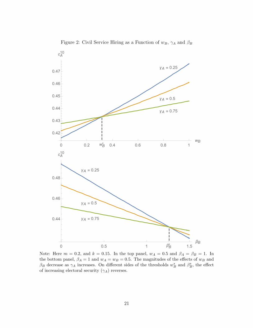
Figure 2: Civil Service Hiring as a Function of wB, γA and βB

γA = 0.25

γA = 0.5

γA = 0.75

0 0.2 wB*

0.4 0.6 0.8 1wB

0.42

0.43

0.44

0.45

0.46

0.47

cA10

γA = 0.25

γA = 0.5

γA = 0.75

0 0.5 1 βB*

1.5βB

0.44

0.46

0.48

cA10

Note: Here m = 0.2, and k = 0.15. In the top panel, wA = 0.5 and βA = βB = 1. Inthe bottom panel, βA = 1 and wA = wB = 0.5. The magnitudes of the effects of wB andβB decrease as γA increases. On different sides of the thresholds w∗B and β∗B, the effectof increasing electoral security (γA) reverses.

21

commitment by both parties to the civil service. For some variables, the static results will be

the same as the dynamic ones. For example, if one party’s cost of hiring civil servants goes

up, both parties will hire more patronage appointees because they are sensitive to their own

costs and those of the other party. This reduces the long run probability of good bureaucracy.

The same is true for policy preferences. If wi increases for either party, both parties have

greater incentive hire civil servants, and thus we should expect a higher probability of good

governance in the long-run if extremism is low.

The more interesting questions about long-run good governance are therefore related to

the electoral environment. When (exogenous) electoral security is increasing for one party

it is decreasing for the other, making it unclear how γA should be related to the long-run

likelihood of good governance. This relationship is all the more complicated by the fact that

the direction of the effect of γA can change with changes in variables like wi and βi.

Since the Markov perfect equilibrium defines a Markov process over states of play, we

can use standard techniques to analyze the long-run behavior of the political system. Recall

that the equilibrium states are denoted (i, n, q), where i is the party in power, n is its term

of office, and q is bureaucratic quality. This defines eight states, as illustrated in Figure 3.

The personnel strategies and re-election probabilities characterized in the previous section

allow us to write an 8 × 8 matrix P of state transition probabilities, where each element

Ps,s′ = Prs | s′ gives the probability of transitioning from state s to state s′ in one period.

For example the probability of transitioning from (i, 1, q) to (i, 2, 1) – that is, for a first-term

party i incumbent with bureaucratic quality q to be re-elected with a good bureaucracy – is

Pi1q,i21 = ρi(c1qi , q)c

1qi . And as no state can repeat itself in consecutive periods, the transition

probability from any state s to itself is Ps,s = 0.

We restrict our analysis to non-corner equilibria where all civil service hiring levels are

interior. The first step is to show the existence of a unique limiting distribution φ = (φA10,

φA20, φA11, φA21, φB10, φB20, φB11, φB21) over the states, which has the property that

limn→∞ Pns,s′ = φs′ for all s, s′. Thus, the long-run probability of state s′ is independent

22

of the starting state s. The following result shows this by invoking the basic limit theorem of

Markov chains, which requires that the underlying Markov process be recurrent, aperiodic,

and irreducible.4

Proposition 5 Limiting Distribution. If cnqi is interior for all states, then there exists a

unique limiting distribution φ over the states of the equilibrium.

The distribution φ allows us to calculate several informative statistics about sample

paths and the distribution of outcomes. Unfortunately, due to the complexity of P (in

particular the fact that there are no absorbing states in the game), calculating φ is not a

trivial exercise. We therefore rely on numerical results generated by Mathematica. In the

remainder of this section we consider the persistence of bureaucratic quality as well as the

long-run probabilities of some sets of states of substantive interest, such as those with good

governance or control by a particular party.

5.1 Persistence of Bureaucratic Quality

A standard calculation in the analysis of discrete Markov Chains is the distribution of initial

“hitting” times for some set of states. This allows us to ask, for instance, the average number

of periods it takes to attain good government from either party starting from a newly elected

party A with low quality bureaucracy (i.e., moving from state (A, 1, 0) to states of the form

(i, n, 1)). This provides a measure of the persistence of bad governance. Likewise, we can

calculate the average time it takes to move to a good bureaucracy, starting from a newly

elected party A with high quality bureaucracy (i.e., moving from state (A, 1, 1) to states of

the form (i, n, 0)).

Figure 4 plots these statistics using the same parameters as Figure 2. The results largely

confirm the intuitions of our short run comparative statics. As wB increases, a new party

A politician is motivated to hire more civil servants, thus hastening the arrival of a good

4For a reference, see Karlin and Taylor (1975).

23

Figure 3: Equilibrium States and Possible Transitions

(A,1,0)(A,2,0)

(A,2,1)

(B,1,0)

(B,1,1)

(A,1,1)

(B,2,0)(B,2,1)

Note: Party A control in red, party B control in blue; light denotes first term and darkdenotes second term.

24

bureaucracy or delaying the arrival of a bad bureaucracy. Electoral advantages also matter:

a good bureaucracy is more likely to persist and a bad one more likely to die when the

electorally advantaged party has the higher public goods motivation wi.

5.2 Sustaining Good Government

Consider the relationship between the electoral environment and good governance, which

corresponds to states of the form (i, n, 1). Figure 5 presents examples of the relationship

between γA and the probability of good bureaucracy under different assumptions about

polarization and the cost of hiring civil servants. The top panel presents the subcase of low

polarization. Civil service hiring and hence good bureaucracy are obviously more likely when

the cost of hiring civil servants for both parties are lower. More interestingly, when these cost

are equal for both parties, the long-run probability of good bureaucracy is maximized when

γA = 0.5. Under these conditions, then, electoral competition fosters good governance. The

role of electoral competition in fostering good governance disappears when the two parties

have asymmetric costs of hiring civil servants. In this case, good governance is enhanced in

low polarization systems if the party with lower costs has an electoral advantage.

The bottom panel presents graphs under the same assumptions about costs, but in a high

polarization environment. The long-run probability of good bureaucracy is now much lower

under any assumptions about costs. There is no discernible impact of electoral competition

when costs are the same for both parties, but good bureaucracy is again most likely when

the party with lower costs has an electoral advantage.

We next ask whether there are partisan differences in bureaucratic quality; that is, which

party is more likely to govern with a good bureaucracy, conditional upon being in power?

The answer is not easily deduced from each party’s hiring decisions because of the delay be-

tween civil service hiring and the realization of good bureaucracies. Moreover, as Proposition

4 establishes, the relationship between civil service hiring and electoral prospects can go in

25

Figure 4: Persistence of Good and Bad Bureaucracy

0.0 0.2 0.4 0.6 0.8 1.0wB

2.0

2.2

2.4

2.6

2.8

3.0

3.2Mean Time

γA = 0.3

γA = 0.5

γA = 0.7

0.2 0.4 0.6 0.8 1.0wB

0.5

1.0

1.5

2.0

2.5

3.0

3.5

Mean Time

γA = 0.3

γA = 0.5

γA = 0.7

Note: Here m = 0.2, k = 0.15, wA = 0.5 and βA = βB = 1. The top panel shows theaverage number of periods before a government is good, starting from a bad governmentand a first term party A politician. The bottom panel shows the average number ofperiods before a government is bad, starting from a good government and a first termincumbent. Good government arrives more quickly and decays more slowly as publicgoods motivations become stronger, and as the more public goods-minded party gains anelectoral advantage.

26

Figure 5: Electoral Competition and the Long-Run Probability of Good Bureaucracy

0.4 0.5 0.6 0.7γA

0.65

0.70

0.75

0.80

0.85

Probability

βA=βB=1.25

βA=βB=0.6

βA=1.25, βB=0.6

βA=0.6, βB=1

(a) Low party system polarization (wA = wB = .9)

0.4 0.5 0.6 0.7γA

0.1

0.2

0.3

0.4

Probability

βA=βB=1.25

βA=βB=0.6

βA=1.25, βB=0.6

βA=0.6, βB=1

(b) High party system polarization (wA = wB = .1)

Note: m = 0.3 and k = 0.1 in both panels. In the top panel, the long-runprobability of good bureaucracy is maximized when elections are com-petitive and costs are equal. In the bottom panel, political polarizationremoves the role of competitive elections. In both panels, the long-runprobability of good bureaucracy is maximized when civil service hiringcosts are low and there is an electoral advantage for the party with lowercivil service hiring costs.

27

either direction. Figure 6 suggests that when parties have symmetric parameters, the elec-

torally disadvantaged party will more often have a good bureaucracy, regardless of whether

polarization is low or high.

Figure 6: Electoral Competition and Bureaucracy Quality by Party

0.3 0.4 0.5 0.6 0.7γA

0.750

0.755

0.760

Probability

Good bureaucracy

Good bureaucracy | A

Good bureaucracy | B

(a) Low party system polarization (wA = wB = .9)

0.3 0.4 0.5 0.6 0.7γA

0.281

0.282

0.283

0.284

0.285

Probability

Good bureaucracy

Good bureaucracy | A

Good bureaucracy | B

(b) High party system polarization (wA = wB = .1)

Note: m = 0.3, βA = βB = 1 and k = 0.1 in both panels. Under both highand low polarization, the electorally disadvantaged party is more likely tobe associated with good bureaucracy, conditional on being in power.

28

5.3 Personnel Policy and Electoral Advantage

The discussion to this point has focused on how electoral politics shapes the long-run proba-

bility of good government. But we can also turn the question around. Personnel decisions by

a party in power affect not only the nature of bureaucracy, but also the electoral prospects

of each party. If one party has a greater incentive to invest in patronage, it can reap an elec-

toral advantage. If a party does this when it has a built-in electoral advantage, the politics

of bureaucracy will entrench advantaged parties. If a party does this when it suffers an elec-

toral disadvantage, it will lessen this disadvantage. We can use the model to consider how

the party system interacts with differential civil service costs to affect a long-run electoral

advantage.

Figure 7 plots the long-run probability that A holds office (corresponding to the states of

the form (A, n, q)) against γA. When party system polarization is high and the costs of civil

service hiring are equal, the effect of strategic personnel decision-making is to increase the

electoral advantage of the favored party. This increase grows larger as the electoral advantage

grows larger, further entrenching the party with the stronger electoral base. This is due to

the relatively strong incentives for patronage politics when party systems are polarized. But

consider what happens when hiring costs are not symmetric, for instance when A has higher

costs of civil service than B. These higher costs of course encourage A to use more patronage

than B, and thus increases the electoral advantage of A when A is favored and decreases the

electoral advantage of B when B is favored (as one would expect given the cross-partials in

Proposition 4). By comparison, when polarization is low, the same basic pattern exists. But

the most striking feature of the figure is how muted these effects are. This suggests that the

politics of personnel will entrench parties that have an electoral advantage, and that this will

be particularly true when the favored party has relatively high costs of hiring civil servants.

However, the extent to which it does so declines as party system polarization declines.

29

Figure 7: Electoral Competition and the Long-Run Probability that A is in Office

0.4 0.5 0.6 0.7γA

0.2

0.4

0.6

0.8

Probability

βA=βB=1

βA=1.2, βB=1

γA

(a) High party system polarization (wA = wB = .1)

0.4 0.5 0.6 0.7γA

0.2

0.4

0.6

0.8

Probability

βA=βB=1

βA=1.2, βB=1

γA

(b) Low party system polarization (wA = wB = .9)

Note: m = 0.3 and k = 0.1 in both panels. Personnel policies help to en-trench the electorally advantaged party, especially under high polarizationand high civil service hiring costs.

30

6 Empirical Implications of the Model

A central assumption in the model is that politicians can make civil service or patronage

appointments in the bureaucracy, and that the more civil servants they hire, the greater the

likelihood that good government will prevail in the future. This assumption undergirds our

argument that politicians are most likely to emphasize civil service hiring when a partic-

ular type of party competition prevails, one where parties that are electoral foes mutually

benefit from good government. The civil service should therefore be least developed when

winning parties have incentives to narrowly target specific groups. This section explores

empirically two questions related to this argument. First, are civil service hiring and good

government related? Second, is civil service hiring least well-developed in countries where

parties narrowly target specific groups for electoral support?

Answering these questions requires measures of good government and civil service, and to

this end we rely on a recent data set by Dahlstrom, Teorell, Dahlberg, Hartmann, Lindberg

and Nistotskaya (2015). The data set is based on a survey of experts in a wide range of

countries that occurred in 2014-15. The experts were asked to place their bureaucracies on

a 1-7 scale on a variety of different dimensions. In using the Dahlstrom et al. data, we have

recoded all variables so that a larger number corresponds to better civil service or better

government. The empirical appendix includes the text of the survey questions that we use

in our analysis. Since our model focuses on democratic electoral competition, we will focus

on countries that have maintained a Polity2 score of 6 or higher (a standard threshold for

coding countries as democratic) for at least five years.

Measuring good government. The theoretical model assumes that good government ben-

efits all parties. We therefore need to consider dimensions of bureaucratic output that do

not have a distributive bias. One dimension is bureaucratic efficiency. If bureaucrats exert

little effort, fail to show up for work, or suffer limitations in their ability to get things done,

everyone (except the bureaucrats) is worse off than they would be if bureaucrats provided

31

services efficiently. Another dimension is neutrality, or unbiasedness. If in providing public

services, bureaucrats favor some groups over others, then citizens and the parties they sup-

port will not benefit equally from bureaucratic output. Finally, good government is honest.

If bureaucrats extract bribes for providing services or embezzle funds from the state, citizens

suffer. And if bribes target some groups of citizens over others, corruption also results in

biased bureaucratic output.

Three different variables in the Dahlstrom et al. data can be used to measure bureaucratic

efficiency. The first (q4 e) is Absenteeism, which takes a higher value when workers do not

skip work without permission. The second (q5 k) is Efficiency, which taps the extent to

which bureaucrats strive to be efficient. And the third (q5 l) is Helpful, which takes a higher

value when bureaucrats strive to be helpful.

There are two variables related to neutrality. Group Bias (q5 f) takes a higher value

when public sector workers are less likely to treat some groups in society differently than

others. Licensing Bias (q5 g) takes a higher value when public sector workers are less likely

to base licensing decisions on personal contacts. Finally, to measure honesty, Bribes (q8 c)

takes a higher value when public sector worker are less likely to grant favors in exchange for

money, while Steals (q8 d) takes a higher value when public sector employees are less likely

to steal or embezzle public monies.

The empirical appendix provides descriptive statistics for these good government vari-

ables, as well as the correlation matrix. Not surprisingly, the variables are strongly related

to each other, with correlations ranging from .63 to .98 among the democracies in our data.

Measuring civil service. How might we measure whether hiring practices are oriented

more towards civil service versus patronage? Scholars often emphasize the institutional

structures for hiring bureaucrats, and in particular whether there exists a formal exam for

hiring bureaucrats (which can limit opportunities to make patronage appointments). This

approach is central to Rauch and Evans (2000), who regard the presence of such an exam

as an important element of Weberian civil service. Exam (q2 d) allows us to measure the

32

importance of merit based exams in hiring, taking a higher value when some form of exam

is central to hiring decisions.

There are a number of reasons to expect that merit exams might be only weakly related

to civil service. Modern personnel system often hire talented individuals using criteria other

than uniform exams, and there are many strategies politicians use to subvert the intended

effects of institutions like merit exams (e.g., Grindle 2012). Thus, we can use a less institu-

tional and more impressionistic approach to measuring civil service: Merit Selection (q2 a)

takes a higher value when experts believe that obtaining a job in the bureaucracy depends

most heavily on skills and merit. It is interesting to note that the two measures are positively

related, but that the correlation is not particularly strong (r = .41), making it worthwhile

to examine which has a stronger relationship with good government.

To this end, we regress each governance quality measure on a set of controls, and on

either Merit Selection or Exam. The controls include the log of GDP/capita (GDP), the

level of democracy (measured using Polity2 ), ethnic polarization (EP),5 an indicator variable

for presidential systems (Presidential), an indicator variable for proportional representation

(PR), the number of years that the county has been democratic (Age Democratic) and

regional indicator variables. Table 1 presents the results from these regressions for the two

measures of civil service. For example, when we regress Absenteeism on Merit Selection and

the controls, the coefficient on Merit Selection is .31 with a standard error of .11.

The regressions that include Merit Selection as the measure of civil service hiring show

a strong, precisely estimated coefficient between this variable and each measure of good

government. The size of the coefficients suggest that a one-unit increase in Merit Selection

on the 7-point scale is often associated with more than a one-half unit increase in the good

government measure. And all coefficients are estimated with standard errors that yield a

p-value of less than .01. By contrast, the regressions using Exam show that this variable has

5EP takes a higher value as society becomes divided into two equally-sized ethnolinguistic groups (seeReynal-Querol 2002). This variable is more closely related to polarization in our model than is the widelyused alternative, ethnolinguistic fractionalization (ELF ).

33

Table 1: Civil Service and Good Government

Measure of Dependent variable: Measure of good governmentcivil service Absenteeism Efficiency Helpful Group Bias Licensing Bias Bribes StealsMerit Selection .31*** .58*** .53*** .43*** .79*** .66*** .64***

(.11) (.09) (.10) (.12) (.14) (.13) (.12)

Exam −.03 .06 .05 .13 .09 .04 .05(.09) (.09) (.08) (.08) (.10) (.10) (.10)

Note. Each cell presents the coefficients from OLS model where the dependent variable is the measureof good government listed at the top of each column and the measure of civil service is listed in theleft-most column. All models also include a number of (unreported) controls which are described in thetext. Robust standard errors are in parentheses. * p < .10, ** p < .05, *** p < .01.

a tiny and very imprecisely estimated coefficient for each measure of good government. In

short, the association between Merit Selection and good government is strong and robust

but the association between Exam and good government is not.

These results are informative for two reasons. First, a key feature of our model is that

the current majority can undo civil service hiring procedures adopted by the previous gov-

ernment. They may do this by adopting new laws or by simply circumventing the intent of

existing procedures. That the associations are stronger for Merit Selection than for Exam

is consistent with the idea that institutional lock-in of civil service hiring is difficult, and

that elected majorities can circumvent the intention of civil service rules meant to tie their

hands. Second, the results have implications for how one should test the relationship be-

tween the electoral context and hiring strategies. In particular, we should expect variables

that encourage civil service appointments to be related to measures of civil service hiring

that are actually associated with good government. Thus, Table 1 strongly suggests that

the theoretical model’s implications for civil service hiring strategies need to tested using

variables like Merit Selection rather than variables like Exam.

We now explore the link between the electoral context and civil service hiring. In the

model, w is the degree to which parties prefer public goods versus private or pork barrel

goods. When w is small it is very difficult to sustain hiring practices that encourage good

34

government. While a range of factors can plausibly affect party preferences, one reasonable

proxy for a party system with low w is one where parties have strong and distinct ethnic

bases of support. When parties rely on different ethnic groups for votes, incumbents have

incentives to serve the narrow interests of the ethnic groups they represent, and also to give

them public sector jobs. Thus, we should expect institutions and practices related to good

government to be negatively correlated with the ethnic basis of support for parties.

We use “Party Voting Polarization” (PVP) to measure the ethnic basis of support for

parties in a country. Given the two-party assumption of the theoretical model, PVP is par-

ticularly appropriate because it increases (a) when political parties tend to have distinctive

bases of support, and (b) when the party system moves toward two main parties (which

is a function of the polarization assumption of the measure). Details of the variable’s con-

struction are found in the empirical appendix and in Huber (2012). The data are taken

from Huber (2012), supplemented by additional observations from the World Values Survey.

There are 74 observations from 42 countries. The surveys are from 1992-2008, prior to the

date of the 2014 civil service survey – at times substantially so – a point we return to below.

Figure 8 shows the scatterplot of the bivariate relationship between PVP and Merit

selection. The expected negative relationship clearly exists, though it is modest in size

(r = −.21). It does not seem driven by any particular outliers. For comparison, the right

panel shows the scatterplot between PVP and Exam. The correlation is positive – the wrong

direction – but extremely weak (r = .11).

Table 2 presents the results of OLS estimations. All models contain EP as a control

variable to ensure that any result are capturing voting behavior, not underlying distributions

of ethnic groups. We also include the controls discussed above, as well as regional fixed effects

(which are not reported in the table). Models 1-3 include each country-year observation for

which we have PVP data, and thus include data as far back as 1992, and include multiple

observations for some countries. The models estimate robust standard errors, clustered by

country, and also include (unreported) year indicator variables.

35

Figure 8: Party Ethnification (PV P ) and Civil Service Hiring

AUSAUSAUSAUS

BGDBGD

BEL BEL

BEN

BRABRA BRA

BGRBGRBGR

CANCANCAN

COLCYP

ESTEST

FINFIN

FRADEU

GHA

GTM

HUN

INDINDIND

IDNISRLVA LVA

LTU

MKDMKDMDG

MEX

MDAMDA MDA

NAM NAM

NZL NZLNZL

PER

ROMSEN

SVK

SVN

ZAFZAF ZAF

ESPESPESPESPESP

SWE

TUR

UKR

USA USA USA USAUSA

URYURY

VENVEN23

45

67

Mer

it se

lect

ion

0 .1 .2 .3 .4Party ethnification (PVP)

AUSAUSAUSAUS

BGDBGD

BEL BEL

BENBRABRA BRA

BGRBGRBGR

CANCANCAN

COL

CYP

ESTEST

FINFIN

FRA

DEU

GHA

GTM

HUN

INDINDINDIDN

ISR

LVA LVA

LTU

MKDMKD

MDGMEX

MDAMDA MDA

NAM NAM

NZL NZLNZL

PER

ROMSEN

SVK

SVN

ZAFZAF ZAF

ESPESPESPESPESP

SWE

TUR

UKR

USA USA USA USAUSA

URYURY

VENVEN

23

45

67

Exam

0 .1 .2 .3 .4Party ethnification (PVP)

Model 1 regresses Merit Selection on each of the right-hand variables except PVP, and

shows that EP actually has a positive coefficient, but one that is not at all precisely estimated.

Model 2 adds PVP, which has a coefficient that is negative and very precisely estimated. The

size of the coefficient suggests that a one standard deviation increase in PVP is associated

with a .31 standard deviation decrease in Merit Selection. By comparison, a one standard

deviation increase in GDP is associated with a .03 standard deviation decrease in Merit

Selection (though this relationship is not precisely estimated). Of the controls other than

EP, only Age Democratic is at all precisely estimated. Model 3 therefore re-estimates model

2, but excluding those variables that seem to have no clear relationship with the dependent

variable in models 1 and 2. PVP continues to have a negative and precisely estimated

coefficient, and the magnitude is larger than in the previous model.

Models 1-3 include an observation for each of the country-years for which data is available

for PVP, which span the period 1992-2008. In some ways, this is not a concern: if we think

that the electoral context influences civil service and that both civil service and voting

patterns evolve slowly over time, it is good that the PVP measures exist for years prior to

the measurement of civil service. Concerns that we have a different number of observations

36

for some countries than others (while our measure of civil service is a constant for each

country) are mitigated to some extent by the fact that the models include year indicators

and estimate robust standard errors clustered by country. It is nonetheless useful to explore

whether the results are robust when we use only one observation per country. To this end, we

create the variable PV PAll, which is the country mean of PVP using all available data. We

then estimate the model with robust standard errors using data from 2008 (the last year for

which we have PVP data). While this approach has the disadvantage that one must choose

an arbitrary year for the cross-section, it has the advantage of assuring us that any results

are not due to overweighting countries that happen to have more surveys. Model 4 provides

the results when all controls are included, and model 5 re-estimates model 4 but omitting

those control variables in model 4 that have no clear relationship with Merit Selection. In

both models, the coefficient on PV PAll remains negative and very precisely estimated.

Finally, to bring the date of the PVP surveys closer to the date of Merit Selection, we

create PV P>2000, which is the country mean of PVP using only data from 2000 or later.

Model 6 includes the full set of controls and model 7 excludes imprecisely measured controls.

In both models, the coefficient for PV P>2000 is negative and precisely estimated. We also

regressed Exam on each of the three measures of PVP (and controls) and in each model (not

reported here) the coefficient for PVP was estimated with very large error.

The analysis therefore provides evidence of a robust negative association between contexts

that encourage narrow, group-based politics and merit-based hiring. There is no evidence

that the electoral context is related to exams, which are not strongly associated with good

government. And there is no negative correlation between ethnic diversity itself – measured

by ethnic polarization – and civil service hiring: only when this diversity is reflected in

electoral competition do we see this relationship.

37

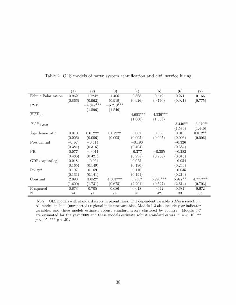
Table 2: OLS models of party system ethnification and civil service hiring

(1) (2) (3) (4) (5) (6) (7)Ethnic Polarization 0.962 1.724* 1.406 0.868 0.549 0.271 0.166

(0.866) (0.962) (0.919) (0.926) (0.740) (0.921) (0.775)PVP −4.342*** −5.210***

(1.596) (1.546)PV PAll −4.603*** −4.530***

(1.660) (1.563)PV P>2000 −3.440** −3.379**

(1.539) (1.440)Age democratic 0.010 0.012** 0.012** 0.007 0.008 0.010 0.012**

(0.006) (0.006) (0.005) (0.005) (0.005) (0.006) (0.006)Presidential −0.367 −0.314 −0.196 −0.326

(0.381) (0.316) (0.404) (0.384)PR 0.077 −0.011 -0.377 −0.305 −0.282

(0.436) (0.421) (0.295) (0.258) (0.316)GDP/capita(log) 0.018 −0.054 0.025 −0.054

(0.165) (0.149) (0.190) (0.246)Polity2 0.197 0.169 0.110 −0.035

(0.131) (0.141) (0.191) (0.214)Constant 2.098 3.052* 4.303*** 3.935* 5.290*** 5.977** 4.777***

(1.600) (1.731) (0.675) (2.201) (0.527) (2.614) (0.703)R-squared 0.673 0.705 0.686 0.648 0.642 0.687 0.672N 74 74 74 41 42 33 33

Note. OLS models with standard errors in parentheses. The dependent variable is Meritselection.All models include (unreported) regional indicator variables. Models 1-3 also include year indicatorvariables, and these models estimate robust standard errors clustered by country. Models 4-7are estimated for the year 2008 and these models estimate robust standard errors. * p < .10, **p < .05, *** p < .01.

38

7 Conclusions

In recent years, there has been growing interest in both the adoption of civil service re-

forms and the somewhat elusive concept of state capacity. To our knowledge, no theoretical

work has yet considered the combination of these features in a framework that allows the

examination of their long-run viability. Our theory of personnel policy attempts to do so

by modeling competing political parties over an infinite horizon. Its main features include

the differentiation between types of bureaucratic personnel, a bureaucratic production func-

tion that affects election outcomes, and relationships between civil service appointments, the

quality of bureaucracy and public goods production.

The model brings into sharp relief the deep challenges associated with creating good

government, which is not something that can be imposed by one party on another, but rather

emerges from the mutual interest of competing political parties. Given that cooperation over

time sustains good government, a party’s civil service hiring will be influenced not simply

by its own preferences, but also by characteristics of the opposition. Expectations about

electoral outcomes are also important. When the other party is moderate and can hire civil

servants inexpensively, civil service hiring is increasing in electoral vulnerability, reflecting

an insurance motive. When this is not true, such hiring is an investment and is therefore

decreasing in electoral vulnerability. The model therefore raises questions about both the

generality and the mechanisms of “lock-in” arguments. Over the long-run, sustaining good

government is enhanced by electoral competition only when party system polarization is low

and the costs of civil service hiring are the same for each party. When these conditions are

not met, good governance is maximized when the advantaged party has lower costs and less

extreme preferences. And electoral incentives associated with personnel policies will entrench

favored parties when these parties have non-centrist preferences.

The analysis suggests several avenues for further research. With respect to the theoretical

model, a difficult but useful extension would be to eliminate the exogenous constraint on the

39

size of the bureaucracy. This would produce predictions about not only the composition of

government, but its size as well. In addition, by including longer time horizons and electoral

constituencies for public goods, the model might shed light on the apparent permanence of

reforms in some countries. More broadly, we believe that the model can serve as a useful

framework for modeling public good investments under electoral competition.

With respect to empirical applications, we have presented evidence using ethnic voting

to describe the link between the nature of electoral competition and civil service hiring. It is

important to consider other ways in which party competition shapes party preferences, and

to examine how such elements of party preferences interact with electoral vulnerability to

influence hiring practices. We have also presented evidence that descriptions of institutional

features of bureaucracy – such as the existence of hiring exams – are inadequate proxies

for civil service. It is important, however, to consider alternatives to experts surveys for

measuring attributes of bureaucratic personnel. Information about bureaucrats themselves

could be very useful in this regard. The model also underlines the importance of thinking

about factors that affect the differential costs of civil service investment across parties. Such

factors may be linked to things like ethnicity if particular ethnic groups are routinely excluded

from civil service positions and ethnic identity is related to vote choice.

40

REFERENCES

Acemoglu, Daron, Davide Ticchi, and Andrea Vindigni. 2011. “Emergence and Persistence

of Inefficient States.” Journal of the European Economic Association 9(2): 177-208.

Azzimonti, Marina. 2011. “Barriers to Investment in Polarized Societies.” American Eco-

nomic Review 101(4): 2182-2204.

Besley, Timothy, and Torsten Persson. 2010. “State Capacity, Conflict, and Development.”

Econometrica 78(1): 1-34.

Besley, Timothy, and Torsten Persson. 2011. Pillars of Prosperity: The Political Economics

of Development Clusters. Princeton, NJ: Princeton University Press.

de Figueiredo, Rui J. P. 2002. “Electoral Competition, Political Uncertainty, and Policy

Insulation.” American Political Science Review 96(2): 321-333.

Folke, Olle, Shigeo Hirano, and James M. Snyder. 2011. “Patronage and Elections in U.S.

States.” American Political Science Review 105(3): 567-585.

Gailmard, Sean, and John W. Patty. 2007. “Slackers and Zealots: Civil Service, Policy

Discretion and Bureaucratic Expertise.” American Journal of Political Science 51(4):

873-889.

Gailmard, Sean, and John W. Patty. 2012. “Formal Models of Bureaucratic Politics.”

Annual Review of Political Science 15: 353-377.

Geddes, Barbara. 1994. Politician’s Dilemma: Building State Capacity in Latin America.

Los Angeles: University of California Press.

Gerber, Elizabeth R., and Clark C. Gibson. 2009. “Balancing Regionalism and Local-

ism: Regional Governance in American Transportation Policy.” American Journal of

Political Science 53(3): 633-648.

Golden, Miriam A. 2003. “Electoral Connections: The Effects of the Personal Vote on

Political Patronage, Bureaucracy and Legislation in Postwar Italy.” British Journal of

Political Science 33: 189-212.

Grindle, Merilee S. 2012. Jobs for the Boys: Patronage and the State in Comparative

Perspective. Cambridge, MA: Harvard University Press.

Grzymala-Busse, Anna. 2003. “Political Competition and the Politicization of the State

in East Central Europe.” Comparative Political Studies 36(10): 1123-1147.

41

Hollyer, James R. 2011. “Patronage or Merit?: Civil Service Boards in US Cities.” Un-

published manuscript, University of Minnesota.

Horn, Murray J. 1995. The Political Economy of Public Administration. New York: Cam-

bridge University Press.

Huber, John D. 2012. “Measuring Ethnic Voting: Do Proportional Electoral Laws Politicize

Ethnicity” American Journal of Political Science 56 (4):9861001.

Huber, John D., and Nolan M. McCarty. 2004. “Bureaucratic Capacity, Delegation, and

Political Reform.” American Political Science Review 98(3): 481-494.

Johnson, Ronald N., and Gary D. Libecap. 1994. The Federal Civil Service and the Problem

of Bureaucracy. Chicago: University of Chicago Press.

Karlin, Samuel, and Howard M. Taylor. 1975. A First Course in Stochastic Processes. San

Diego, CA: Academic Press.

Knack, Stephen, and Philip Keefer. 1995. “Institutions and Economic Performance: Cross-

Country Tests Using Alternative Institutional Measures.” Economics and Politics 7(3):

207-227.

Knott, Jack H., and Gary J. Miller. 1987. Reforming Bureaucracy: The Politics of Insti-

tutional Choice. Englewood Cliffs, NJ: Prentice-Hall.

Krause, George A., David E. Lewis, and James W. Douglas. 2006. “Political Appointments,

Civil Service Systems, and Bureaucratic Competence: Organizational Balancing and

Executive Branch Revenue Forecasts in the American States.” American Journal of

Political Science 50(3): 770-787.

La Porta, Rafael, Florencio Lopez-de-Silanes, Andrei Shleifer, and Robert W. Vishny. 1999.

“The Quality of Government.” Journal of Law, Economics, and Organization 15(1):

222-279.

Lavertu, Stephane. 2013. “Issue-specific Political Uncertainty and Policy Insulation in

Federal Agencies.” Journal of Law, Economics, and Organization 29: 145-177.

Lewis, David E. 2008. The Politics of Presidential Appointments: Political Control and

Bureaucratic Performance. Princeton: Princeton University Press.

Moe, Terry, 1989. “The Politics of Bureaucratic Structure.” In ed. John E. Chubb and Paul

E. Peterson, Can the Government Govern? Washington, DC: Brookings Institution.

42

Montalvo, Jose G., and Marta Reynal-Querol. 2005. “Ethnic Polarization, Potential Con-

flict and Civil War.” American Economic Review 95(3): 796–816.

Mueller, Hannes. 2015. “Insulation or Patronage: Political Institutions and Bureaucratic

Efficiency.” B.E. Journal of Economic Analysis & Policy 15(3): 961-996.

Nath, Anusha. 2015. “Bureaucrats and Politicians: How Does Electoral Competition

Affect Bureaucratic Performance?” Unpublished manuscript, Boston University.

Pollock, James K. 1937. “The Cost of the Patronage System.” Annals of the American

Academy of Political and Social Science 189: 29-34.

Ramseyer, J. Mark. 1994. “The Puzzling (In)dependence of Courts: A Comparative

Approach.” The Journal of Legal Studies 23(2): 721-747.

Rauch, James E. 1995. “Bureaucracy, Infrastructure, and Economic Growth: Evidence

from U.S. Cities During the Progressive Era.” American Economic Review 85(4): 968-

979.

Rauch, James, and Peter B. Evans. 2000. “Bureaucratic Structure and Bureaucratic

Performance in Less Developed Countries.” Journal of Public Economics 75(1): 49-71.

Reid, Joseph D., and Michael M. Kurth. 1989. “Public Employees in Political Firms: Part

B, Civil Service and Militancy.” Public Choice 60(1): 41-54.

Reynal-Querol, Marta. 2002. “Ethnicity, Political Systems, and Civil Wars.” Journal of

Conflict Resolution 46(1): 29-54.

Roett, Riordan. 1999. Brazil: Politics in a Patrimonial Society. Westport, CT: Praeger.

Ruhil, Anirudh V.S., and Pedro J. Camoes. 2003. “What Lies Beneath: The Political

Roots of State Merit Systems.” Journal of Public Administration Research and Theory

13(1): 27-42.

Stephenson, Matthew C. 2003. “When the Devil Turns: The Political Foundations of

Independent Judicial Review.” The Journal of Legal Studies 32(1): 59-89.

Ting, Michael M. 2011. “Organizational Capacity.” Journal of Law, Economics, and Or-

ganization 27(2): 245-271.

Ting, Michael, Olle Folke, Shigeo Hirano, and James Snyder. 2013. “Elections and Reform:

The Adoption of Civil Service Systems in the U.S. States.” Journal of Theoretical

Politics 25(3): 363-387.

43

Ujhelyi, Gergely. 2014. “Civil Service Reform.” Journal of Public Economics 118: 15-25.

44

THEORETICAL APPENDIX

Proof of Proposition 1. Let Ωi denote a party i first-term incumbent’s conjectured payoff

from a subsequent period in which she is not re-elected and the bureaucracy is good, where in

equilibrium Ωi = ui(c11j , 1). Additionally, let c1q

i (Ωi) denote the optimal level of civil service

hiring for a newly elected party i politician, given Ωi. Differentiating the objective (3) with

respect to c produces:

dEUi(c|s)dc

= ((1−q)m(1−2c) + γi)[ui(c

10j , 0)−Ωi−ui(c20

i , 0)+ui(c21i , 1)

]− ui(c10

j , 0) +

Ωi + (1−q)m(ui(c10j , 0)−ui(c20

i , 0)−k)− 2βi + (1+q)wi − 4c+ 3. (10)

Substituting in expressions (5)-(7) into (10) and solving this first order conditions yields

the following solutions for c10i (Ωi) and c11

i (Ωi):

c10i (Ωi) =

1

2+

3w2i γi −m(8k + w2

i + (1− 2βi)2 − 2wi(1 + 2βi))+

wi(8 + (6− 4βi)γi) + 8(1− 2βi + (1− γi)Ωi)

32 + 2m(3w2i + wi(6− 4βi)− 8Ωi)

, (11)

c11i (Ωi) =

1

2+

3w2i γi + wi(16 + (6− 4βi)γi) + 8(1− 2βi + (1− γi)Ωi)

32. (12)

Expressions (11) and (12) are identical to (8) and (9) in the proposition, respectively, so

it only remains to solve for Ωi. Using the definition of Ωi, we have the following relationships:

Ωi = ui(c11j (Ωj), 1)

Ωj = uj(c11i (Ωi), 1).

Solving for Ωi yields:

Ωi =wi(96−64βj+12w2

j (1−γi) + wj(88−16βj(1−γi)− 16βiγi + 3w2i γ

2i + 2wiγi(8 + 3γi−2βiγi)))

(8(16− wiwj(1− γi)γi)).

45

We next verify that the objective is concave. Substituting from (5)-(7) into (3), the

second order condition is:

m

4(8Ωi + wi(4βi − 3wi − 6))− 4.

By the bounds on the stage game payoffs, Ωi < 1, and thus this expression is negative.

Proof of Comment 1. We show that c1qi is increasing in wi. The results for βi are derived

identically and are therefore omitted.

First consider when a party i politician inherits a bad bureaucracy. Let G(c) = dEUi(c|s)dc

be her first order condition, as given by equation (10). By the implicit function theorem,

at a maximum,∂c10i∂x

= −∂G∂x∂G∂c

for any exogenous parameter x. Since ∂G∂c

< 0 (this is the

second order condition, established in the proof of Proposition 1), sign∂c10i∂x

= sign∂G∂x

(c10i ).

Evaluating ∂G∂wi

(c10i ) produces:

∂G

∂wi=

2αi − (2c10Am− γi)(3wi + 2αi − 1) + 2βi + 2m(wi + αi + βi)

2(αi + βi).

Given αi + βi = 2, this partial derivative is positive if z = 4 + 2c10i m− (3wi + 2αi)(2c

10i m−

γi)+2m(wi+2)−γi > 0. Since z is linear in m and m is bounded by 0 and γi, it is sufficient

to check that z positive at these bounds. At m = 0, z = 4 − γi + (3wi + 2αi)γi > 0. At

m = γi, z = 4 + (3 + 5wi + c10i (2− 6wi − 4αi) + 2αi)γi > 0 for all possible c10

i ∈ [0, 1].

Next consider when a party i politician inherits a good bureaucracy. Evaluating the

derivative of c11i directly produces:

∂c11i

∂wi=

12w2j (1− γi)2 + 32(7 + 2αj(1− γi) + 3wiγi + 2αiγi)−

wj(1− γi)(3w2i γ

2i − 16αj(1− γi)− 16αγi − 56)

2(16− wiwj(1− γi)γi)2.

Each term in this expression is positive, and thus∂c11i∂wi

> 0.

46

Proof of Proposition 2. We first establish the result for∂c10A∂wB

. Let G(c) = dEUA(c|s)dc

be A’s first order condition, as given by equation (10). Following the implicit function

theorem argument in the proof of Comment 1, we show that ∂G∂wB

(c10A ) > 0. Since G(c)

depends on ΩA (i.e., the value to A of the public goods produced by B if B wins and the

bureaucracy is good, as defined in the proof of Proposition 1) and ΩA depends on wB, we

have ∂G∂wB

(c10A ) = ∂G

∂wB+ ∂G

∂ΩA

∂ΩA

∂wB. Evaluating each component gives:

∂G

∂wB= 0

∂G

∂ΩA

= 1 + (2c10A − 1)m− γA

∂ΩA

∂wB=

wA(96wB(1− γA)− 3wAw2B(1− γA)2γA+

4(3w2Aγ

2A + 4αB(1− γA)(4 + wAγA) + 8(7 + 2αAγA) + 2wAγA(7 + 2αAγA))

2(16− wAwB(1− γA)γA)2).

Noting that ∂G∂ΩA

> 0 by our assumptions on m and γi, these expressions imply that

sign∂c10A∂wB

= sign∂ΩA

∂wB. This derivative is clearly positive given that 96wB(1−γA)−3wAw

2B(1−

γA)2γA > 0 and all other terms are positive.

For∂c10A∂βB

, we perform the analogous exercise. Since ∂G∂βB

= 0, we have sign∂c10A∂βB

= sign∂ΩA

∂βB,

which evaluates to 2wA(γA−5)16−wA(1−γA)γA

< 0.

For c11A , by analogous arguments, sign

∂c11A∂wB

= sign∂ΩA

∂wB, which we have shown is positive,

and sign∂c11A∂βB

= sign∂ΩA

∂βB, which we have shown is negative. This establishes the result.

Proof of Proposition 3. For both levels of bureaucratic quality, Comment 1 shows that

party A’s civil service hiring is increasing in wA, and Proposition 2 shows that it is increasing

in wB. Thus, civil service hiring is increasing in w = wA = wB.

Proof of Proposition 4. It can easily be shown (see Figure 1, for example) that there

exist cases where∂c1qA∂γA

> 0 and∂c1qA∂γA

< 0.

Throughout, let G(c) = dEUA(c|s)dc

be A’s first order condition, as given by equation (10),

and let ΩA denote the value to A of the public goods produced by B if B wins and the

47

bureaucracy is good, as defined in the proof of Proposition 1.

(i) We characterize conditions under which∂c10A∂γA

> (<) 0 for wB sufficiently small (large).

Using the implicit function theorem, it is straightforward to show that∂c10A∂γA

> (<) 0 iff

∂G∂γA

(c10A ) > (<) 0. Taking the total derivative, we have ∂G

∂γA(c10A ) = ∂G

∂γA+ ∂G

∂ΩA

∂ΩA

∂γA. Evaluating

each component gives:

∂G

∂γA=

3w2A + wA(6− 4βA)

16− ΩA

∂G

∂ΩA

= 1 + (2c10A − 1)m− γA

∂ΩA

∂γA=

wAwB [3γ2Aw

3AwB − 2γAw

2((2βA − 11)γAwB + 48) + 64(4βA − 4βB + 3wB)−4wA [32γA(βB−βA)−16βB+88+3(1−γA)2w2

B+wB (4βAγ2A−4βB(1−γA)2−44γA+22)]]

8(16− (1− γA)γAwAwB)2.

We next provide two bounds on ∂G∂γA

(c10A ), and show that these bounds are decreasing in

wB. From the expressions above it is clear that ∂G∂γA

(c10A ) is linear in µ = (−1 + 2c10

A )m, and

hence ∂2G∂γA∂wB

(c10A ) is also linear in µ. Since γA + γB = 1, µ is bounded by max−γA, γA− 1

and minγA, 1 − γA. Abusing notation slightly, we verify that ∂2G∂γA∂wB

∣∣∣µ=γA−1

< 0 and

∂2G∂γA∂wB

∣∣∣µ=γA

< 0, and therefore ∂G∂γA

(c10A ) must be bounded from above and below by two

functions that are decreasing in wB.

∂2G∂γA∂wB

∣∣∣µ=γA−1

has a positive denominator and is therefore negative if it has a negative

numerator. This condition reduces to:

+ 4(3w2Aγ

2A + 4αB(1− γA)(4 + wAγA) + 8(7 + 2αAγA) + 2wAγA(7 + 2αAγA)) > 0.

96wB(1− γA)− 3wAw2B(1− γA)2γA

This must be true given that 96wB(1− γA)− 3wAw2B(1− γA)2γA > 0 and each term in the

second line of the expression is positive.

Next, ∂2G∂γA∂wB

∣∣∣µ=γA

has a positive denominator and is therefore negative if it has a negative

48

numerator. This condition reduces to:

4wA(3w2B(1−γA)2 + 8(7+αB(2−4γA)+4αAγA)+2wB(7+2αB(1−γA)2−14γA−2αAγ

2A)) < 0

(−16− wAwB(1− γA)γA)(64(3wB − 4αA + 4αB) + 3w3AwBγ

2A + 2w2

AγA(wB(7 + 2αA)γA − 48)−wB(16αB(1− γA) + 3w2

Aγ2A + 8(7 + 2αAγA) + 2wAγA(8− γA + 2αAγA))

]+

−wA(1− γA)γA(16− wAwB(1− γA)γA)[64αB + 12w2

B(1− γA)− 32+

2αB(1− γA)2 − 14γA − 2αAγ2A))

−wB(16− wAwB(1− γA)γA)(192 + 3w3Aγ

2A + 2w2

A(7 + 2αA)γ2A − 8wA(7 + 3wB(1− γA)2+

3w2Aγ

2A + 8(7 + 2αAγA) + 2wAγA(8− (1− 2αA)γA))

−(16 + wAwB(−1 + γA)γA)2(24wB(1− γA) + 16αB(1− γA)+

Of the four terms in this expression, only the last can be positive. The sum of the first

and last term is linear in αB, and thus the entire expression is negative if this sum is negative

at αB = 0 and at αB = 3/2, which is true for all possible parameter values.

These bounds imply that ∂G∂γA

(c10A ) > 0 for wB sufficiently low, and ∂G

∂γA(c10A ) < 0 for wB

sufficiently high. Define the functions G : R → R and G : R → R, where G(wB) = ∂G∂γA

,

evaluated at µ = γA and arbitrary values of wB, and G(wB) = ∂G∂γA

evaluated at µ =

γA− 1, and arbitrary values of wB. By the preceding derivation, both of these functions are

decreasing in wB. Define w∗B andw∗B as follows:

w∗B =

0 if minG(0), G(0) < 0

wB if minG(wB), G(wB) = 0 and wB ∈ (0, 1)

1 if minG(1), G(1) > 0.

w∗B =

0 if maxG(0), G(0) < 0

wB if maxG(wB), G(wB) = 0 and wB ∈ (0, 1)

1 if maxG(1), G(1) > 0.

Thus, ∂G∂γA

(c10A ) > 0 if wB < w∗B, and ∂G

∂γA(c10A ) < 0 if wB > w∗B. The comparative statics

result for∂c10A∂γA

follows from the implicit function theorem.

49

(ii) To prove the result for βB, we differentiate ∂G∂γA

(c10A ) with respect to βB, yielding:

−

2wA ((1− γA)2wAw2B((2c10

A − 1)m+ 1)−4wB((2c10

A − 1)m((2γA − 1)wA + 4) + (1− γA)((γA − 1)wA + 8))− 64)

(16− (1− γA)γAwAwB)2

Since the denominator is clearly positive, ∂G∂γA

(c10A ) is increasing in βB if the numerator is

negative. To verify this, we define µ = (2c10A − 1)m and substitute this into the numerator,

noting that µ is bounded between−1 and 1. Then taking the derivative of the numerator with

respect to µ yields 2wAwB (wA ((1− γA)2wB − 8γA + 4)− 16). This expression is negative,

and thus the numerator is maximized at µ = −1. Substituting this into the numerator

produces an upper bound of 8wA (wB (8γA + γ2AwA − 4)− 16), and thus the numerator is

negative for all possible values of µ.

Now define the function G : R→ R, where G(βB) = ∂G∂γA

, evaluated at c10A and arbitrary

values of βB. We define β∗B as follows:

β∗B =

1/2 if G(1/2) < 0

βB if G(βB) = 0 and βB ∈ (1/2, 2)

1 if G(1) > 0.

Thus, ∂G∂γA

(c10A ) < 0 if βB < β∗B, and ∂G

∂γA(c10A ) > 0 if βB > β∗B. The comparative statics

result for∂c10A∂γA

follows from the implicit function theorem.

(iii) We calculate the derivatives of c11A directly.

∂c11A∂γA

, in terms of ΩA, is:

1

32(16− (1− γA)γAwAwB)2

[w3Aw

2Bγ

2A(1− γA) ((4β − 6)γA − 3γAwA − 16)−

4w2A

(3(γA − 1)3w3

B + 2(1− γA)w2B

(−2βAγ

2A + 2βB(1− γA)2 + 22γA − 11

)−

8(1− γA)wB(βB(4γA − 2)− 6γA + 11)− 192) +

64wA(−16βA − 3(1− γA)w2

B − 4(1− γA)wB(βA − βB) + 24)]− ΩA

4. (13)

50

Differentiating (13) with respect to wB produces:

wA8(16− (1−γA)γwAwB)3

[12(γA−1)γ3

Aw3AwB + 512(βA(4γA−2) + (4βB − 6wB)(1−γA)− 11)+

γAw2A

(3(γA−1)3w3

B − 8(1−γA)wB(2βB(1−γA)2 − 2βAγ

2A + 22γA − 11

)− 576γA + 384

)+

16wA(8(6βAγ

2A − 4βAγA + βB

(−6γ2

A + 8γA − 2)− 22γA + 11

)+ 9(1− γA)2w2

B−

2(1− γA)wB(2βAγA(1− 2γA) + 4βB(1− γA)2 + 33γA − 22

))].

The denominator of this expression is obviously positive, and so the sign of the cross partial

equals the sign of the numerator. It is straightforward to verify that the numerator must be

negative, and therefore∂2c11A

∂γA∂wB< 0.

For∂2c11A∂γA∂βB

, differentiating (13) with respect to βB produces:

wA (64− (1− γA)2wAw2B + 4(1− γA)wB(8− (1− γA)wA))

2(16− (1− γA)γAwAwB)2.

This expression is obviously positive, as claimed.

Proof of Proposition 5. We show that the Markov chain with transition probability

matrix P is irreducible and aperiodic. Since the chain is finite, these features imply that it

is recurrent and therefore has a unique limiting distribution.

To show irreducibility it is sufficient to demonstrate that all states communicate with

a distinguished state, which we designate (A, 1, 0). By our assumptions on γi and m, all

re-election probabilities are interior. By assumption, all cnqi are also interior. Thus P can be

depicted as follows, where ‘+’ indicates Ps,s′ ∈ (0, 1):

A10 A20 A11 A21 B10 B20 B11 B21

51

A10 0 + 0 + + 0 + 0

A20 + 0 + 0 + 0 + 0

A11 0 + 0 + + 0 + 0

A21 + 0 + 0 + 0 + 0

B10 + 0 + 0 0 + 0 +

B20 + 0 + 0 + 0 + 0

B11 + 0 + 0 0 + 0 +

B21 + 0 + 0 + 0 + 0

It is clear that Pinq,A10 > 0 for all states except (A, 1, 0) and (A, 1, 1). Since PA10,A20 > 0

and PA11,A20 > 0, all states can reach (A, 1, 0) in two periods. Next, from (A, 1, 0) only

(A, 1, 0), (A, 1, 1), (B, 2, 0) and (B, 2, 1) cannot be reached in one period. But since

PA10,B10 > 0 and all four of these states are reachable from (B, 1, 0) in one period, we

conclude that all states communicate.

To show aperiodicity, we first observe that irreducibility implies that all states have the

same period. Since (A, 1, 0) can return to itself in two periods (e.g., through (B, 1, 0)) and

in three periods (e.g., through (B, 1, 0) and (B, 2, 0)), the state (A, 1, 0) is aperiodic, and

hence the Markov chain is aperiodic.

52

8 EMPIRICAL APPENDIX

Text of Expert Survey Questions

Questions from Dahlstrom et al. (2015) are of the form: “Thinking about the country you

have chosen, how often would you say the following occurs today?” Answers were provided

on a scale from 1 (almost never) to 7 (almost always).

Variables related to good government

Bureaucratic efficiency

q4 e. Public employees are absent from work with-out permission. (Abensteeism)

q5 k. Public sector employees strive to be efficient. (Efficiency)

q5 l. Public sector employees strive to help citizens. (Helpful)

Neutrality

q5 f. When deciding how to implement policies in individual cases, public sector employees

treat some groups in society unfairly. (Group Bias)

q5 g. When granting licenses to start up private firms, public sector employees favor appli-

cants with whom they have strong personal contacts. (Licensing Bias)

Honesty

q8 c. Public sector employees grant favors in exchange for bribes, kickbacks or other ma-

terial inducements. (Bribes)

q8 d. Public sector employees steal, embezzle or misappropriate public funds or other state

resources for personal or family use. (Steals)

Variables related to civil service hiring practices

q2 a. When recruiting public sector employees, the skills and merits of the applicants decide

who gets the job. (Merit Selection)

q2 d. Public sector employees are hired via a formal examination system. (Exam)

53

The PVP Measure

For each pair of parties, the measure calculates the difference in their ethnic bases of support.

It then sums these differences using a polarization metric (where polarization scores are a

measure that increases as one moves toward two equal sized groups).

Formally, the measure is defined as follows. First, for each pair of political parties i and

j in a state, we calculate the distance between their electoral bases of support, rij. Formally,

rij =

√√√√1

2

G∑g=1

(P ig − P

jg )2, (14)

where P ig and P j

g are the proportion of supporters of parties i and j who come from group g,

and there are G groups. The maximum rij is 1, which occurs when all of party i’s support

comes from one group, and all of party j’s support comes from another group. The minimum

distance is zero, which occurs when the proportion of support that comes from each group

for party i is the same as the proportion of support that comes from each group for party j.

In general, as the distribution of groups supporting any two parties becomes more similar,

rij will decline.

Second, we use the vote shares of parties to aggregate the rij’s, yielding the system-level

measure of PVP :

PV P = 4N∑i=1

N∑j=1

pip2j rij, (15)

where pi is the proportion of the vote received by party i and there are N parties.

The pip2j term in the definition of PVP ensures that holding the ethnic distance between

parties constant (and assuming it is non-zero), the measure increases as the party system

moves toward two parties of equal size.

54

The Data

The PVP data are from 1995-2008.

Table 3: Summary statistics of good government variables in democracies

count mean sd min maxAbensteeism 71 4.878 1.118 2.333 6.875Efficiency 70 3.976 1.077 2.000 6.286Helpful 70 4.182 1.084 2.000 6.286Group Bias 70 4.366 1.036 1.667 6.167Licensing Bias 70 4.231 1.402 1.250 6.750Bribes 71 4.394 1.510 1.667 7.000Steals 71 4.558 1.489 1.750 7.000

Table 4: Bivariate correlations of good government variables in democracies

Variables Abensteeism Efficiency Helpful Group Licensing Bribes StealsBias Bias

Abensteeism 1.000Efficiency 0.629 1.000Helpful 0.707 0.917 1.000Group Bias 0.632 0.711 0.753 1.000Licensing Bias 0.734 0.831 0.824 0.776 1.000Bribes 0.746 0.860 0.873 0.765 0.930 1.000Steals 0.783 0.837 0.865 0.761 0.913 0.980 1.000

55