civil 3d, the modern
DESCRIPTION
The 3D in Civil 3D could standfor Design, Delineation, Depiction because of its strengths in developing curvilinearand rectilinear geometry objects.TRANSCRIPT

Chapter Objectives
After reading this chapter, the student should know/be able to:• Understand the mathematics behind the Civil 3D geometry tools.• Understand distances; bearings; information on traverses used for estab-
lishing control on projects; and formulas for circles, arcs, triangles, andlines.
• Use Civil 3D for creating and editing these geometry items.• Use the many Transparent commands that are in Civil 3D.• Understand how to develop, label, and edit alignments and parcels.
INTRODUCTION
Civil 3D is a modern curvilinead. What is a curvilinead? It is an instrumentthat draws curvilinear and rectilinear objects. The 3D in Civil 3D could standfor Design, Delineation, Depiction because of its strengths in developing curvi-linear and rectilinear geometry objects. This chapter begins with some of theformulas needed to design geometry and discusses curvilinear linework gener-ation, roadway alignment, and parcel creation, editing, and drafting. The abil-ity to modify these data and the development of curvilinear 2D geometry (Lines,Arcs, Spirals), parcels, alignments, and labels are discussed in detail.
REVIEW OF FUNCTIONS AND FEATURES TO BE USED
This chapter uses engineering functions to compute angles, slopes, and dis-tances. Civil 3D has many tools for creating lines and curves, and this chapterexamines how these are then used to create disciplinary objects such as align-ments and parcels.
COMPUTATIONS OF LINES AND THEIR ANGLES
In a vector-based program, points create lines. Points occupy a position con-sisting of only an X coordinate, a Y coordinate, and a Z coordinate. A linear con-nection of the dots occurs with a clear start, a distance, and direction. Refer toFigure 4-1 for a line starting at 0, 0 and continuing through a point of 7.5, 2.5.
The points can be Civil 3D points or simply just AutoCAD points or pickson the screen, but they are points nevertheless. When drawing lines in AutoCAD,you can easily find out information about them by using the LIST command.
124Civil 3D, the ModernCurvilinead
WARDMC04_0131713507 6/23/06 5:10 PM Page 145

146 Chapter 4 Civil 3D, the Modern Curvilinead
But where does the LIST command compute its results from? Can theseresults be accomplished by hand, using manual techniques? You certainlyshould be able to reproduce these results using manual techniques just incase you want to check the computer. One of the worst things that someoneusing a computer can do when asked, “How do you know that the value iscorrect?” is to say, “Because the computer said so.” A better response wouldbe: “I know this is a correct estimate of the value based on my knowledge ofthe software’s algorithms and the data I developed.” It is necessary to knowthe engineering and mathematical formulas behind these algorithms, andeach chapter in this text explores them. This chapter discusses linear andcurvilinear computations.
Example 4-1: Find the Angle of a Two-Dimensional Line from the X Axis
To find the angle from the X axis of the two-dimensional line with the samecoordinate values as shown in Figure 4-1, follow this process.
The angle then is computed as: (ATAN((ABS)slope)) � ATAN(1) � 45°
Example 4-2: Find the Angle of a Three-Dimensional Line from the X Axis
To find the angle from the X axis of the three-dimensional line with thesame coordinate values as shown in Figure 4-1, follow this process.
The angle then is computed as: (ATAN((ABS)slope)) � ATAN(0.70710678) �35.254°The formula for a line � Y � mX � b was discussed in Chapter 3 underPoint Basics.The Y coordinate � the slope of the line times the X coordinate plus the yintercept. Therefore, in Figure 4-1 m � .333, X � 7.5, and b � 0; Y � 2.5.
DISTANCES AND BEARINGS
Distances and bearings are used to show course and lengths for many itemssuch as parcel lines, boundaries, alignments, pipelines, and so forth. The bear-ing has four quadrants, each no larger than 90 degrees. It always starts ateither north or south and is followed by the angle and then the direction towhich it turns, which is either east or west. See Figure 4-2.
Slope = ¢Z >2A2+ B2
= (5 - 10)>(7.0710678) = 0.70710678
Slope = ¢Y>¢X = (20 - 15)>(10 - 5) = 5>5 = 1
Figure 4-1 A vector
WARDMC04_0131713507 6/23/06 5:10 PM Page 146

Chapter 4 Civil 3D, the Modern Curvilinead 147
3D LINEWORK USES SLOPE DISTANCES FOR DISTANCEMEASUREMENT
Distances measured can include horizontal lengths, vertical lengths, slope
distances, or vertical angles. Figure 4-3 shows what these are in establishingdata connecting Point A to Point B.
Figure 4-2 Bearing quadrants
Example 4-3: Computing the Difference in Height Between Rods
As shown in Figure 4-4,
Difference in Elevation = 7.21 - 2.63 = 4.58¿
Rod reading = 2.63¿
Rod reading = 7.21¿
Figure 4-3 Slope distances
Slope Distances—The dis-
tance measured along an
incline
Figure 4-4 Computing the difference in height between rods
WARDMC04_0131713507 6/23/06 5:10 PM Page 147

148 Chapter 4 Civil 3D, the Modern Curvilinead
CONTROL SURVEYS
Control Surveys establish reference points and reference lines for preliminaryand construction surveys. Vertical reference points called benchmarks are alsoestablished. These are then tied into state coordinate systems, property lines,road centerlines, or arbitrary grid systems. The various types of tie-in methodsare shown in Figure 4-5.
Control Survey—The “monu-
mentation” for projects
• Type A, rectangular tie-in, is also known as a right angle offset. Remem-ber in Chapter 3 how many commands assisted us in developing thesePerpendiculars?
• Type B, polar tie-in, is also known as the angle/distance technique.
• Type C, intersection tie-in, uses two angles from a baseline to locate aposition.
Example 4-4: Stationing
Distances along baselines are called stations, as in Figure 4-6. Right anglescan be achieved from the baseline. The distance along this right angle iscalled an offset.
Station 2 � 36.517 is 236.517′ from the intersection of Elm and Pine.The left corner of the building is 236.517′ from Elm and 40.01′ at a 90 degreeangle from Pine.
Figure 4-5 Tie-in methods
Figure 4-6 Stationing
Example 4-5: Doubling the Angle
A surveying technique to enhance precision when shooting data in the fieldis called Doubling the Angle. The angles are effectively shot and computedtwice for each interior angle. Due to human error, ambient condition error,or equipment error, these measures are often slightly different. So the
WARDMC04_0131713507 6/23/06 5:10 PM Page 148

Chapter 4 Civil 3D, the Modern Curvilinead 149
surveyor often creates a mean of the two angles, anticipating that the meanangular error is less than any one of the angles independently.
Station Direct Angle Double Angle Mean
A 101-24-00 202-48-00 101-24-00
B 149-13-00 289-26-00 149-13-00
C 80-58-00 161-57-00 80-58-30
D 116-20-00 232-38-00 116-19-00
E 92-04-00 184-09-00
Total Degrees 538-119-00 � 539-59-00 (Is this correct?)
The total number of degrees within a closed polygon depends on the numberof sides and is computed using the following formula. ANGULAR CLOSURE �(N � 2) � 180; therefore, our polygon � 3 � 180 � 540-00-00. So subtractingthese yields 540-00 minus 539-59-00 � 01′-00′′ ERROR. See Figure 4-7.
92-04-30
Figure 4-7 Polygons
VECTOR DATA AND FORMULAS
As a refresher in order to fully understand the computations that the Civil 3Dsoftware performs, the following information is provided along with examples.Formulas for computing the following data manually follow:
Circles
• Radius, Perimeter, Area
Right triangles
• Lengths of sides, Interior angles
Curvilinear Objects Including Arcs, Circular Curves, and Spirals
• Arc definition, Chord definition
• Define the components of an arc
• Formulas for computing Arc Length (L), Radius (R), Chord length (C),Mid-ordinate chord distance (M), External secant (E), and Tangentlength (T)
• Define the components of a spiral
• Types of horizontal curves
Secant—Geometry term
WARDMC04_0131713507 6/23/06 5:10 PM Page 149

150 Chapter 4 Civil 3D, the Modern Curvilinead
Circle Formulas
Right Triangle Definitions and Formulas
Sides
Note
Example 4-6: Triangles
If the right triangle in Figure 4-8 has a 27.5′ base and a height of 38.7′, howwould you find:
B° = Tan-1(a>b) or Sin-1(a>c) or Cos-1(b>c)A° = Tan-1 (b>a) or Sin-1(b>c) or Cos-1(a>c)A° = 180° - 90° - B° or, 90° - B° : B° = 90° - A°
A + B + C = 180°Cos = Adjacent>HypotenuseSin = Opposite>HypotenuseTan = Opposite>Adjacent
c2= (a2
+ b2)b2
= (c2- a2)
a2= (c2
- b2)a2
+ b2= c2
Area = � * r2Perimeter = 2 * � * r or, � * Diameter2 Pi radians = 3601 radian = 180>�Pi radians = 180°Radius = 1>2 * Diameter
Figure 4-8 Triangles
1. The angle B.
0.1569 * 60 = 9.414 = 54 - 36 - 9
0.60261522 * 60 = 36.1569
B = Tan-1(opp>adj) = Tan-1 (38.7>27.5) = 54.60261522
WARDMC04_0131713507 6/23/06 5:10 PM Page 150

Chapter 4 Civil 3D, the Modern Curvilinead 151
2. The remaining angle of the triangle:
3. The length of the hypotenuse:
4. The area of the triangle:
5. What is the closest distance from C to any point along the hypotenuse?
6. Where does the shortest distance line intersect the hypotenuse in rela-tion to point A?
We know two sides of the new triangle so,
Because a right triangle is being divided into smaller right triangles, theinterior always remains the same as with the original triangle.
Example 4-7: A Practical Problem
See Figure 4-9. A homeowner wants to remove the Ex. Tree and put a wellthere. County regulations say the well must be 50� from the drain field and25� from the house. Does it work?
a = 2(c2- b2) = 2((27.5)2 - (22.42)2) = 15.92¿
a2+ b2
= c2 and that c = 22.42 and b = 27.5
* Sin (54.6026) = 22.42¿
If X = Y>Z, then Y = X * Z and Z = Y>X, then 27.5We know that Sin (54.6026) = opp>hyp
We know angle B = 54.6026°
(27.5 * 38.7)>2 = 532.13 ft2
c = 2((27.5)2 + (38.7)2) = 47.48¿
90 - 54.6026 = 35.40
Figure 4-9 Locating a proposed well—1
The measured distance from the tree to the house � 26′; OK. The dis-tance from the drain field to the house is 32.5′. Distance from the tree tothe drain field Not OK. See Figure 4-10.
Suggested new location for well could be:
An alternative #2 might be: b = 2(502- 262) = 42.71, say, 43¿
An alternative #1 might be: a = 2(c2- b2) = 2(502
- 32.502) = 38¿
= 2(32.52+ 262) = 41.60;
WARDMC04_0131713507 6/23/06 5:10 PM Page 151

152 Chapter 4 Civil 3D, the Modern Curvilinead
From the corner of the drain field looking at the corner of the house, whatis the angle to locate the proposed well?
For alternative #2,
CURVILINEAR OBJECTS—ARCS, CIRCULAR CURVES, AND SPIRALS—DEFINITIONS AND FORMULAS
Another aspect of drawing is the ability to compute curves and arcs. Arcs aredefined as those curvilinear objects that have a fixed radius, and curves arethose objects that may have a fixed radius but may also be dynamic. Spiralsand parabolas fall into the curve category.
Some specific formulas for computing arc data and spiral data need to bediscussed in detail before moving toward automated solutions.
For arcs there are two definitions, the Arc definition (Figure 4-11) and theChord definition (Figure 4-12). The Arc definition is the most widely used and typ-ically used by highway designers and other land development staff. It is also calledthe “Roadway definition.” The Chord method is called the “Railway definition.”
= Cos-1 (32.5>50) = 49.45° = Sin-1 (40>50) = 53.13°
A = Tan-1 (40>32.5) = 50.9°
Figure 4-10 Locating a proposed well–2
Figure 4-11 The Arc definition
WARDMC04_0131713507 6/23/06 5:10 PM Page 152

Chapter 4 Civil 3D, the Modern Curvilinead 153
The Arc method of curve calculation occurs where the degree of curve ismeasured over an arc length of 100′. The formulas are:
The Chord method of curve calculation occurs where the degree of curve ismeasured over a chord length of 100’. The formulas are:
Circular Curves
According to Figure 4-13,
If Dc = 1°, then R = 5729.648 units.R = 50>Sin (1>2)Dc, where Dc is in degrees.Sin (Dc>2) = 50>R
And R = 5729.578>Da. If Da = 1°, then R = 5729.578 m and � = 3.14159 Á
And R = 5729.578>Da. If Da = 1°, then R = 5729.578¿ and � = 3.14159 Á
R = 5729.578>Da. If Da = 1°, then R = 5729.578 units and � = 3.14159 Á
Da = 5729.578>R.Da = 36000>(2 * � * R), orDa>100 = 360°>(2 * PI * R),
Figure 4-12 The Chord definition
Figure 4-13 Circular Curves
L = Length of curveT = Tangent length
PT = Point of TangencyPI = Point of Intersection
WARDMC04_0131713507 6/23/06 5:10 PM Page 153

154 Chapter 4 Civil 3D, the Modern Curvilinead
Arc Formulas
Note in the formulas, the difference between the letter I and the number 1.
Example 4-8: Basic Curve Formulas
Example 4-9: Curve Application
Two highway tangents intersect with a right intersection angle I � 12-30-00at station 0 � 152.204 m. If a radius of 300 m is to be used for the circu-lar curve, prepare the field book notes to the nearest minute in order to layout the curve with 20 m staking.
Solution:
Station of PT = 0 + 184.799 m+L = + (0 + 65.450)Station of PC = 0 + 119.349-T = - (0 + 32.855)Station of PI = 0 + 152.204
= 65.450 mL = RI�>180 = (300)(12.50)(�)>180
= 32.855 mT = R * Tan (I>2) = 300 * Tan (6°15¿)
C = 2(95.49) * Sin (45>2) = 73.08 M = 95.49 * (1 - (Cos (I>2))) = 95.49 * (1 - .92387) = 7.268
* 0.08239 = 7.867= 95.49((1>Cos(I>2)) - 1) = 95.49 R = 5729.578>60 = 95.49; E
75 = (100 * 45)>Da, therefore Da = (100 * 45)>75 = 60.0000M = 7.27, Da = 60.0000
= 39.55, C = 73.09, E = 7.87, If I = 45, L = 75, then R = 95.49, T
M = E * Cos (I>2) R = 50>(Sin (D>2))
M = R(1 - Cos (I>2)) E = T * Tan (I>4)
E = R((1>Cos (I>2)) - 1) (R - M)>R = Cos (I>2)
C = 2R * Sin (I>2) R>(R + E) = Cos (I>2)
T = R * Tan (I>2)R = 5729.578>Da°
L = 100 * I°>Da° L = RI (where I is in radians), or RI�>180
PCC = Point of Compound Curvature (not shown)PRC = Point of Reverse Curvature (not shown)M = Middle ordinate distanceC = Chord lengthR = RadiusI = Deflection angle (Delta)PC = Point of CurvaturePOC = Point on CurveD = Dc degree of curve, chord definitionD = Da degree of curve, arc definitionE = External distance
Note:The deflection angle for achord length of 20 m from the
PC is (20/L)(I/2). The fieldnotes are set up in the following table.
WARDMC04_0131713507 6/23/06 5:11 PM Page 154

Chapter 4 Civil 3D, the Modern Curvilinead 155
Station Chord Dist from PC Point Deflection Angle
0 � 184.799 65.450 PT 6-15-00
0 � 180 60.651 5-47-30
0 � 160 40.651 3-52-55
0 � 140 20.651 1-58-19
0 � 120 0.651 00-03-44
0 � 119.349 0 PC 00-00-00
Procedure: 180 � 119.349 � 60.651
(60.651/65.45) � 6.25 � 5.7917° � 5-47-30°
Example 4-10: Centerline Curve
Find the arc distance for the roadway centerline shown in Figure 4-14.If this were a complete circle, the perimeter would be:
Shortcut = (angle * R2)/114.59 = 9424.91 ft2Partial area = angle>360 * �r2Shortcut = (angle * R)>57.30 = 94.25¿
Therefore, 27°>360° * 1256.64 = 94.25¿.2�r = 2�200 = 1256.64¿
Figure 4-14 Arc distance
Example 4-11: Miscellaneous Applications for Curve Solutions
These concepts can be used in widely varying problems. Here is an exam-ple of a pipe problem in which you need to compute flow through a pipe. A48′′ diameter RCP is flowing 14′′ deep (Figure 4-15). What are the area offlow and wetted perimeter?
Figure 4-15 Flow through a pipe
WARDMC04_0131713507 6/23/06 5:11 PM Page 155

156 Chapter 4 Civil 3D, the Modern Curvilinead
Figure the angles of the triangle and base width (across water surface).
Cos angle � Adjacent/Hyponteuse
Then, the total angle across the water surface The base width Then, the total width of the water surface Figure the flow area. Area (triangle) � ((base � height)/2) � 2; the 2scancel out.
This information could be used in Mannings formula as follows.The RCP is sloped at a grade of 5%. We know that the n � 0.013 for Mannings
friction coefficient. Then,
Spiral Definitions and Formulas
Spirals are used to create a smooth transition as one travels from a tangent toa curve and then back out to a tangent again. Figure 4-16 shows the parame-ters for coming into a spiral. The parameters are the same for leaving a spiral.
Q = 1.55 * a1.554.57
b2>3
* 10.05 *
1.4860.013
= 19.26 cfs.
Q = A * aA
Wpb
2>3* 2S * a
1.486nb
The wetted perimeter = angle * R/57.30 = 130.95614 * 2/57.30 = 4.57¿
Flow area = 4.57 - 3.02 = 1.55 sq. ft2Area of water = angle * R2>114.59 = 130.9614 * 22/114.59 = 4.57 ft23.64 * 0.83 = 3.02 ft2
= 2 * 1.82 = 3.64¿
= 2(c2- a2) = 1(22 - 0.832) = 1.82¿
= 2 * 65.4807 = 130.9614°
Angle = Cos - 1 (0.83¿>2.0¿) = 65.4807°
Figure 4-16 Spirals
R = Radius of circular curve T = Total tangent length Dc = Circular curve delta Ds = Spiral delta angle D = Total deflection angle PI = Point of Intersection CS = Curve to spiral SC = Spiral to Curve TS = Tangent to spiral point
WARDMC04_0131713507 6/23/06 5:11 PM Page 156

Chapter 4 Civil 3D, the Modern Curvilinead 157
curve referred to the straight end of the spiral
Formulas for Approximate Solutions to Spiral Problems
Types of Horizontal Curves
The curves shown in Figure 4-17 illustrate the various types of curves that arein the civil engineering business. The broken back curve is usually not allowedby review agencies because the tangent is not tangent to the curve.
ST = (Sin (1>3 * �)) * L>Sin (�)LT = (Sin (2>3 * �)) * L>Sin (�)
P = Y>4K = X>2
X = 1(L2 - Y2)X2 = L2 - Y2
Y = L * Sin (�)Y>L = Sin (�)
SPI = Spiral PI
K = Abscissa of the PC of the shifted circular P = Offset of the tangent line to the PC of the shifted curve Y = Total ”Vertical” Spiral Length X = Total ”Horizontal” Spiral length ST = Short tangent LT = Long tangent L = Length of spiral
Figure 4-17 Types of horizontal curves
CIVIL 3D’S DEFAULT ANGULAR SYSTEM
In Civil 3D, the default angle definitions occur using the Cartesian system, inwhich the positive X direction is to the right on the screen or monitor and neg-ative X is to the left. Positive Y is up the screen and negative Y is down. Posi-tive Z is basically in the user’s face with negative Z going into the monitor.Angles increase counterclockwise from 0° along the X axis to 360°, back to theX axis. Figure 4-18 shows a 90° angle from the X axis.
Broken Back Curve—Non-
tangent data
WARDMC04_0131713507 6/23/06 5:11 PM Page 157

158 Chapter 4 Civil 3D, the Modern Curvilinead
Another default in AutoCAD and Civil 3D is that the units for the anglestend to be set to decimal degrees and 0 places of precision. These should alsobe set up prior to usage so that the desired angles and criteria are to the com-pany’s liking. Some people prefer to use degrees, minutes, and seconds as theangle units type, and the precision is usually set to, at least, the nearest sec-ond. If the user prefers to use decimal degrees then the precision should be toat least four places. The software converts any output listings to the units theuser sets. So if the units are set to decimal degrees and a LIST command is is-sued, the CAD system responds with decimal degrees as part of the listing. Ifthe units are set to degrees, minutes, and seconds, then the system respondsaccordingly. These can be flipped at any point in the working session to achievethe desired units reporting.
CONVERTING DECIMAL DEGREES TO D-M-S
If the user must perform these computations manually, here are some exam-ples of converting angular units from decimal degrees to degrees, minutes, andseconds.
Example 4-12: Angular Conversions Decimal Degrees to D-M-S
49.5566° breaks down to 49° and 0.5566 of a degree. Then, multiply0.5566 degree � 60 (minutes per degree) to get the number of minutes,which � 33.396 minutes. Now you have 33 minutes and 0.396 of aminute. Then multiply 0.396 minute � 60 seconds per minute to get thenumber of seconds, which is � 23.76 seconds. Therefore, 49.5566° �49°�33′�23.76′′.
Example 4-13: Angular Conversions D-M-S to Decimal Degrees
To convert DMS 49°�33′�23.76′′ to decimal degrees perform the follow-ing: 23.76′′/60 (seconds per minute) � 0.396 minute. Then add the 33′to the 0.396′ to get 33.396′. Then divide 33.396’ by 60 (minutes perdegree) and get 0.5566 degree. Then add the 49° to the 0.5566 to get49.5566°.
ANGLES IN CIVIL ENGINEERING
Now that you can compute the angles of linework manually and based on theCartesian coordinate system, it is time to discuss in more depth how to talkabout angles in terms that civil engineers and surveyors use. This industryuses angles to describe many things, such as property line directions, roadcenterline directions, and construction instructions for stakeout. Some of thetypes of important angles to understand are interior angles, azimuths, bear-ings, cardinal directions, deflection angles, and turned angles.
Figure 4-18 Angles in AutoCAD
WARDMC04_0131713507 6/23/06 5:11 PM Page 158

Chapter 4 Civil 3D, the Modern Curvilinead 159
Figure 4-19 Interior angles
An azimuth can be measured from either the North or South. The Northazimuth measures angles from the North axis, in a clockwise direction to360°. The South azimuth measures angles from the South axis, clockwiseto 360°.
Bearings (Figure 4-20) measure a heading and are broken into four quad-rants: North, South, East, and West. Each quadrant has 90°. The quadrantusually referred to as quadrant 1 is the North-East quadrant and measuresfrom North and turns toward the East. Therefore, a bearing of N 45°�30′30′′ Eis located by facing North and turning toward the East an angle of45°�30′�30′′. Quadrant 2 is South-East and begins by facing South and turn-ing the angle toward the East. Quadrant 3 is South-West and also begins byfacing South but turns toward the West. Quadrant 4 is North-West, begins byfacing North and turning the angle toward the West.
Figure 4-20 Bearings
There are also angles known as cardinal directions, which are North,South, East, and West, routinely seen in describing the heading of a hurricane.“Hurricane Ivan is heading North-North-West,” which is halfway between Northand North-West. In degrees that would be N 22°�30′00′′ W.
Figure 4-21 illustrates a person standing at Point B, looking forward at theangle defined from Point A to Point B and then turning 28°�16′�51′′ to theright to get to Point C. This shows deflection angles.
Figure 4-21 Deflection angles
Interior angles (Figure 4-19) measure the angle between two linear objects.The angle can be acute or obtuse.
WARDMC04_0131713507 6/23/06 5:11 PM Page 159

160 Chapter 4 Civil 3D, the Modern Curvilinead
Figure 4-22 illustrates a person standing at Point B, looking back at PointA, and then turning 208°�16′�51′′ to the right to get to Point C. This showsturned angles.
Figure 4-22 Turned angles
On the subject of angles, there are two other types of angle measurement,one called Grads and another called Radians. A Grad is 1/400th of a circle,where North is what would be zero, East is 100 g, South is 200 g, West is 300 g,and back to North is 400 g. This angular system is used in some internationalcountries and by the United States Department of State. A Radian is 180°/�and is often used in computer programming and in the calculation of some arcformulas.
Exercise 4-1: Units
1. Begin the Civil 3D software.2. Draw a line from 11,7 to 38, 18 and terminate the command.3. Then type LIST at the command prompt. The software responds as
follows.Select objects:
Select the object, hit <Enter> and this listing will display.LINE Layer: “0”Space: Model spaceHandle = 3F2from point, X = 11.0000 Y = 7.0000 Z = 0.0000to point, X = 38.0000 Y = 18.0000 Z = 0.0000Length = 29.1548, Angle in XY Plane = 22Delta X = 27.0000, Delta Y = 11.0000, Delta Z = 0.0000
Note the angle of 22 degrees. Is it an even 22°?
4. Next, at the command prompt, type UN for Units to bring up the Units
dialog box. See Figure 4-23.5. Note under the Angle Type pop-down window are the supported angle
types. Decimal Degrees is the default. The default Precision is set to 0;
Figure 4-23 Units dialog box
WARDMC04_0131713507 6/23/06 5:11 PM Page 160

Chapter 4 Civil 3D, the Modern Curvilinead 161
hence there is no precision for display beyond the nearest degree. Setthe Precision to 4 and hit OK.
6. Type LIST again, select the line, and hit <Enter>. Notice that the angleshown now is 22.1663 degrees.
7. Next, at the command prompt, type UN again to bring up the Units
dialog box.8. Under the Angle Type pop-down window choose Deg/Min/Sec and hit
OK. Type LIST again, select the line, and hit <Enter>. Notice that theAngle in XY Plane � 22d9′59′′.
9. Next at the command prompt type UN again to bring up the Units dialogbox.
10. Under Angle Type pop-down window, choose Surveyor’s Units and hitOK. Type LIST again, select the line, and hit <Enter>. Notice that theAngle in XY Plane is a bearing of N 67d50′1′′ E.
Many Geometry commands can be performed using the Parcels andAlignments menus. Discussion of other tools as well will follow but here is abrief explanation of the menu pull-downs for Parcels and Alignments.
The Parcels pull-down menu (Figure 4-24) commands include:
Figure 4-24 The Parcels pull-down menu
Create By Layout... invokes the Parcel Creation Layout toolbar.
Create From Objects allows for creating new parcels from entities.
Create ROW allows for creating automatic offsets for Right of Way creation.
Edit Parcel Segments... invokes the Layout toolbar for editing parcels thatalready exists.
Edit... invokes the Layout toolbar for editing parcels that already exist.
Edit User Defined Properties... allows editing of user defined propertiesthat are attached to parcels.
Add Labels... adds specific labels to parcels.
Tables allow for creating property tables of lines, arcs, and so on.
Renumber/Rename Parcels allows the same.
The Alignments pull-down menu (Figure 4-25) commands are:
Create By Layout... invokes the Alignment Creation Layout toolbar.
Create From Polyline allows for creating new alignments from polylines.
Edit Alignment Geometry... invokes the Layout toolbar for editing align-ments that already exist.
Edit... invokes the Layout toolbar for editing alignments that already exist.
to AutoCADNEW
2007
to AutoCADNEW
2007
WARDMC04_0131713507 6/23/06 5:11 PM Page 161

162 Chapter 4 Civil 3D, the Modern Curvilinead
Add Labels... adds specific labels to alignments.
Tables allow for creating alignment tables of lines, arcs, and so on.
Reverse Alignment Direction allows the same.
GEOMETRY COMPUTATIONS
Now that the chapter has covered the basic and fundamental mathematicsbehind curvilinear and rectilinear geometry, discussion proceeds with thecapabilities of Civil 3D in these areas. Again, enormous functionality existswithin AutoCAD alone, and because it is a prerequisite to know AutoCAD, cov-erage of those routines within Civil 3D follows.
In addition to investigating some of the primitive geometry tools, the toolsfor creating parcels and alignments are also explored.
THE TRANSPARENT COMMANDS TOOLBAR
To begin, type in Toolbar at the command prompt. In the Toolbar dialog box,choose the Toolbars tab. In the menu group Window, select Civil. In theToolbars window, turn on the check for Transparent commands. If it is alreadyon, leave it on. Hit Close. The Transparent Commands toolbar should be dis-played on the screen, as in Figure 4-26.
Figure 4-26 The Transparent toolbar
Figure 4-25 The Alignment pull-down menu
You can use Transparent commands within other commands that needdata entry consisting of multiple points such as the AutoCAD LINE command.These can be used just like the AutoCAD Transparent commands by precedingthem with an apostrophe. You can also pick them as needed from the toolbar.A user can set a series of points using that data entry format because it re-mains in that data entry mode until you change it or exit.
The Civil Transparent commands are used to enter values based on infor-mation that can be supplied when you are prompted for a radius, a point, or adistance. Most of these commands are used to specify point locations within
WARDMC04_0131713507 6/23/06 5:11 PM Page 162

Chapter 4 Civil 3D, the Modern Curvilinead 163
J
They are fun to use and provide excellent visuals as you work with them.The command definitions from left to right across the toolbar are described asfollows with the accompanying abbreviation that can be typed in as the com-mand is being used.
• ‘AD—Angle and Distance
• ‘BD—Bearing and Distance
• ‘ZD—Azimuth and Distance
• ‘DD—Deflection Angle and Distance
• ‘NE—Northing and Easting
• ‘GN—Grid Northing and Grid Easting
• ‘LL—Latitude and Longitude
• ‘PN—Point Number
• ‘PA—Point Name (alias)
• ‘PO—A Point in a Drawing
• Three new commands were added to the toolbar. They include: ProfileStation from Plan, Profile Station and Elevation from Plan and ProfileStation and Elevation from COGO Point. These commands prompt forand allow for the user to select information for the profile by referring tothe plan view of the alignment. These can be beneficial in that an impor-tant location can be identified using plan view objects that can not beseen when viewing the profile. This could be the location of a horizontalutility manhole perhaps.
• ‘SO—Station and Offset
• ‘SS—Side Shot From a Point
• Transparent command filters exist at this location in the toolbar. Theseallow for selecting point information by Point Number, by selecting
to AutoCADNEW
2007
Job skills will benefit because these routines save hours of manual computation for designers.
another operation, such as the creation of property lines for parcel data. Thesecommands provide great flexibility of obtaining information from data alreadyexisting within the drawing without forcing you to accumulate the informationahead of time. This allows you to calculate the location for a point from a vari-ety of angles and distances.
WARDMC04_0131713507 6/23/06 5:11 PM Page 163

164 Chapter 4 Civil 3D, the Modern Curvilinead
the Point anywhere the point data are visible, or via a Northing/Easting entry.
• ‘PSE—Station and Elevation in a Profile View
• ‘PGS—Grade and Station in a Profile View
• ‘PGL—Grade and Length in a Profile View
• ‘MR—An Object’s Length
• ‘ML—An Object’s Radius
Exercise 4-2: The ‘AD Command
You now explore how these commands work. Let us begin with the ‘AD
command. This command allows you to build linework using a turnedangle and distance (Figure 4-27).
Figure 4-27 Turned angle and distance
This command can be used to describe a traverse based on an occupied point, a backsight,turned angles, and distances.TIP
1. Open the drawing called Chapter-4-Geometry.Dwg.2. Using the V for View command, highlight the view called Geom-A, hit
Restore, and then hit OK. You draw linework using turned angles anddistances from the line visible on the screen.
3. Type L for Line. Follow the prompts:4. LINE Specify first point: Using an Endpoint Osnap pick the north-
ern end of the line in the view.5. Specify next point or [Undo]: Type ‘AD or select the first icon on the
Transparent Commands toolbar.
TIP
WARDMC04_0131713507 6/23/06 5:11 PM Page 164

Chapter 4 Civil 3D, the Modern Curvilinead 165
8. >>Specify angle or [Counter-clockwise]: Type 128.0996
9. >>Specify distance: 75
10. Resuming LINE command.11. Specify next point or [Undo]: (922.563 1060.79 0.0)12. Specify next point or [Undo]:13. Current angle unit: degree, Input: DD.DDDDDD (decimal)14. >>Specify angle or [Counter-clockwise]: 279.8302 (Figure 4-28).
Figure 4-28 Turned angle of 279.8302
15. >>Specify distance: 100
Resuming LINE command.
16. Specify next point or [Undo]: (1020.06 1038.57 0.0)17. Specify next point or [Close/Undo]:
Current angle unit: degree, Input: DD.DDDDDD (decimal)
18. >>Specify angle or [Counter-clockwise]: 233.3313 (Figure 4-29).19. >>Specify distance: 75
20. Resuming LINE command.21. Specify next point or [Close/Undo]: (1050.37 969.965 0.0)
6. >>Specify ending point or [.P/.N/.G]: Using an Endpoint Osnappick the southern end of the line in the view.
7. Current angle unit: degree, Input: DD.DDDDDD (decimal)
If the prompt shows DD.MMSS then you can type 128d5′58.56′′ or change the drawingsettings so it asks for DD.DDDDDD. This is done by going to the Toolspace, clicking onthe Settings tab, right clicking on the drawing name, and choosing Edit Drawing Set-
tings. Choose the Ambient Settings tab and expand the Angle. Change the Value for
the Format to the desired setting.
TIPTIP
WARDMC04_0131713507 6/23/06 5:11 PM Page 165

166 Chapter 4 Civil 3D, the Modern Curvilinead
22. Specify next point or [Close/Undo]:23. Current angle unit: degree, Input: DD.DDDDDD (decimal)24. >>Specify angle or [Counter-clockwise]: *Cancel*
Resuming LINE command.
25. Specify next point or [Close/Undo]: <ESC>26. Save your file with the same name and a suffix of your initials.
Notice the almost video game–style graphics that appear to help you throughthe computations. The yellow marker simulates a station setup while the green“rodman” is placed at the backsight and the red “rodman” is placed at the fore-sight location. The red arc indicates that the computations are using a turnedangle from the backsight to the foresight.
Exercise 4-3: The ‘BD Command
This command allows you to build linework using a bearing anddistance.
Figure 4-29 Turned angle of 233.3313
Job skills will benefit from the use of this command because surveyors routinely draw property andeasement linework using distances and bearings.J
1. Continue in the same drawing or open the drawing you just saved.2. Using the V for View command, highlight the view called Geom-A,
hit Restore, and then hit OK. You draw linework using a bearingand distance from where you left off in the previous command. Youcan also use the line visible on the screen if you did not perform thelast example. Of course your results may vary from the figure some-what.
3. Command: L4. LINE Specify first point: Using an Endpoint Osnap pick the end
of the last line you drew in the previous example. It is near 1050, 969.
WARDMC04_0131713507 6/23/06 5:11 PM Page 166

Chapter 4 Civil 3D, the Modern Curvilinead 167
Figure 4-30 The Northeast quadrant
7. A reminder displays: Current direction unit: degree, Input:
DD.MMSSSS (decimal dms)
8. >>Specify bearing: 41.3329, indicates a bearing angle of 41 degrees,33 minutes, and 29 seconds.
9. >>Specify distance: 75
10. Resuming LINE command. Specify next point or [Undo]: (1100.121026.09 0.0)
11. Specify next point or [Undo]: Quadrants - NE = 1, SE = 2, SW =3, NW = 4
12. >>Specify quadrant (1-4): 3 Current direction unit: degree, Input:
DD.MMSSSS (decimal dms)
13. >>Specify bearing: 16.1907
14. >>Specify distance: 80
15. Resuming LINE command. Specify next point or [Undo]: (1077.64949.309 0.0)
16. Specify next point or [Close/Undo]: Quadrants - NE = 1, SE = 2,SW = 3, NW = 4
17. >>Specify quadrant (1-4): <ESC>18. Save your file with the same name and a suffix of your initials.
Exercise 4-4: The ‘ZD Command
This command allows you to build linework using an azimuth (from North)and distance (Figure 4-31).
5. Specify next point or [Undo]: Type ‘BD or select the second icon onthe Transparent Commands toolbar. A reminder displays: Quadrants -NE = 1, SE = 2, SW = 3, NW = 4
6. >>Specify quadrant (1-4): 1, for Northeast quadrant (Figure 4-30).
If your jurisdiction requires the use of Azimuth (or South Azimuth), this command assistsin laying out deed information.TIPTIP
WARDMC04_0131713507 6/23/06 5:11 PM Page 167

168 Chapter 4 Civil 3D, the Modern Curvilinead
1. Continue in the same drawing or open the drawing you just saved.2. Using the V for View command, highlight the view called Geom-A, hit
Restore, and then hit OK. You draw linework using a bearing and dis-tance from where you left off in the previous command. You can alsouse the line visible on the screen if you did not perform the last exam-ple. Of course your results may vary from the figure somewhat.
3. Command: L
4. LINE Specify first point: Using an Endpoint Osnap pick the end ofthe last line you drew in the previous example. It is near 1077, 949.
5. Specify next point or [Undo]: Type ‘ZD or select the third icon on theTransparent Commands toolbar. Current direction unit: degree, Input: DD.MMSSSS (decimal dms)
6. >>Specify azimuth: 260.2256
7. >>Specify distance: 100
8. Resuming LINE command. Specify next point or [Undo]: (979.048932.602 0.0)
9. Specify next point or [Undo]: Current direction unit: degree, In-put: DD.MMSSSS (decimal dms)
10. >>Specify azimuth: <ESC>11. Save your file with the same name and a suffix of your initials.
Exercise 4-5: The ‘DD Command
This command allows you to build linework using a deflection angle and adistance (Figure 4-32).
1. Continue in the same drawing or open the drawing you just saved.2. Using the V for View command, highlight the view called Geom-A, hit
Restore, and then hit OK. You draw linework using a bearing and dis-tance from where you left off in the previous command. You can also usethe line visible on the screen if you did not perform the last example. Ofcourse your results may vary from the figure somewhat.
3. Command: L4. LINE Specify first point: Using an Endpoint Osnap pick the end of
the last line you drew in the previous example. It is near 979, 932.
Figure 4-31 Linework using a North Azimuth
WARDMC04_0131713507 6/23/06 5:11 PM Page 168
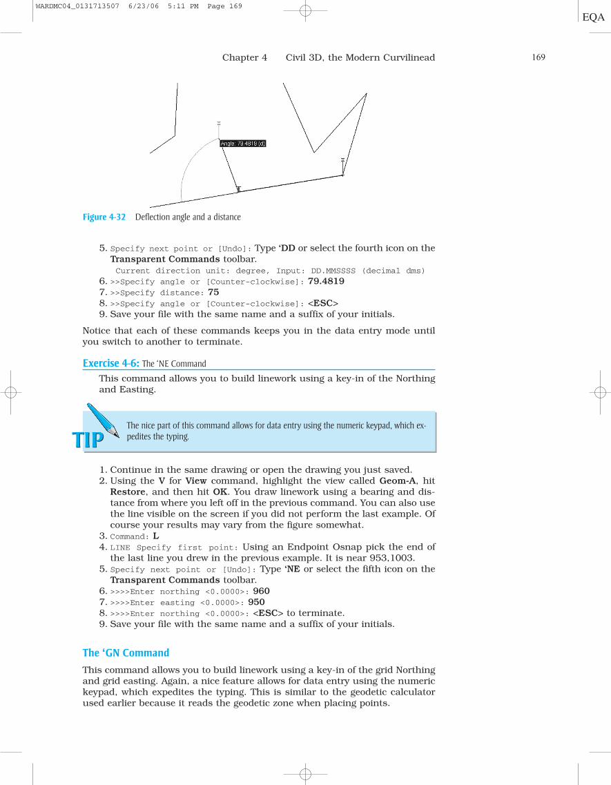
Chapter 4 Civil 3D, the Modern Curvilinead 169
5. Specify next point or [Undo]: Type ‘DD or select the fourth icon on theTransparent Commands toolbar. Current direction unit: degree, Input: DD.MMSSSS (decimal dms)
6. >>Specify angle or [Counter-clockwise]: 79.4819
7. >>Specify distance: 75
8. >>Specify angle or [Counter-clockwise]: <ESC>9. Save your file with the same name and a suffix of your initials.
Notice that each of these commands keeps you in the data entry mode untilyou switch to another to terminate.
Exercise 4-6: The ‘NE Command
This command allows you to build linework using a key-in of the Northingand Easting.
Figure 4-32 Deflection angle and a distance
The nice part of this command allows for data entry using the numeric keypad, which ex-pedites the typing.TIP
1. Continue in the same drawing or open the drawing you just saved.2. Using the V for View command, highlight the view called Geom-A, hit
Restore, and then hit OK. You draw linework using a bearing and dis-tance from where you left off in the previous command. You can also usethe line visible on the screen if you did not perform the last example. Ofcourse your results may vary from the figure somewhat.
3. Command: L
4. LINE Specify first point: Using an Endpoint Osnap pick the end ofthe last line you drew in the previous example. It is near 953,1003.
5. Specify next point or [Undo]: Type ‘NE or select the fifth icon on theTransparent Commands toolbar.
6. >>>>Enter northing <0.0000>: 960
7. >>>>Enter easting <0.0000>: 950
8. >>>>Enter northing <0.0000>: <ESC> to terminate.9. Save your file with the same name and a suffix of your initials.
The ‘GN Command
This command allows you to build linework using a key-in of the grid Northingand grid easting. Again, a nice feature allows for data entry using the numerickeypad, which expedites the typing. This is similar to the geodetic calculatorused earlier because it reads the geodetic zone when placing points.
TIP
WARDMC04_0131713507 6/23/06 5:11 PM Page 169

170 Chapter 4 Civil 3D, the Modern Curvilinead
The ‘LL Command
This command allows you to build linework using a key-in of the latitude andlongitude. This is similar to the geodetic calculator used earlier because itreads the geodetic zone when placing points.
Exercise 4-7: The ‘PN Command
This command allows you to build linework using a key-in of the pointnumber.
This command is not limited to simply typing a point number; it can also connect multi-ple points using commas and apostrophes. For instance, you can draw a polyline by start-ing at a point number of, say, 100 and for the remaining vertices of the polyline you canrefer to points in the file by 101-110, 100, which will draw linework through the consecu-tive points 101 through 110 and connect back to the starting point of 100.
TIP
1. Continue in the same drawing or open the drawing you just saved.2. Using the V for View command, highlight the view called Geom-A, hit
Restore, and then hit OK. You draw linework using a bearing and dis-tance from where you left off in the previous command. You can alsouse the line visible on the screen if you did not perform the last exam-ple. Of course your results may vary from the figure somewhat.
3. Command: L
4. LINE Specify first point: Type ‘PN or select the eighth icon on theTransparent Commands toolbar.
5. >>Enter point number <1>: <Enter>6. Resuming LINE command. Specify first point: (826.126 943.344 0.0)7. Specify next point or [Undo]:8. >>Enter point number <1>: 2
9. Resuming LINE command. Specify next point or [Undo]: (908.0381000.71 0.0)
10. Specify next point or [Undo]:11. >>Enter point number <2>:<ESC> to terminate.12. Save your file with the same name and a suffix of your initials.
Exercise 4-8: The ‘PO Command
This command allows you to build linework using a pick of a point on thescreen without snapping to it. You can pick any visible portion of the pointor its text attributes.
1. Continue in the same drawing or open the drawing you just saved.2. Using the V for View command, highlight the view called Geom-A, hit
Restore, and then hit OK. You draw linework using a bearing and dis-tance from where you left off in the previous command. You can alsouse the line visible on the screen if you did not perform the last exam-ple. Of course your results may vary from the figure somewhat.
3. Command: L
4. LINE Specify first point: Type ‘PO or select the tenth icon on theTransparent Commands toolbar.
5. Select point object: Simply pick on the word UNIT for Point 2.6. Resuming LINE command. Specify first point: (908.038 1000.71 0.0)7. Specify next point or [Undo]:8. >> Select point object: Hit <Enter>
TIP
WARDMC04_0131713507 6/23/06 5:11 PM Page 170

Chapter 4 Civil 3D, the Modern Curvilinead 171
9. >> Specify next point or [Undo]: Type in 950,960
10. Resuming LINE command.11. >> Specify next point or [Undo]: <ESC> to terminate.12. Save your file with the same name and a suffix of your initials.
Exercise 4-9: The ‘SO Command
This command allows you to build linework using a station and offset(positive for right and negative for left) from an alignment.
This routine is useful because it also works inside other AutoCAD commands and refer-ences the alignment in question. It can be used to draw manholes at a station offset froman alignment.TIPTIP
1. Continue in the same drawing or open the drawing you just saved.2. Using the V for View command, highlight the view called Geom-B, hit
Restore, and then hit OK. You see a shot alignment in the view. Drawlinework using a station and offset of this alignment.
3. Type CIRCLE or pick it from the Draw toolbar.4. CIRCLE Specify center point for circle or [3P/2P/Ttr (tan tan
radius)]: Type ‘SO or select the eleventh icon on the Transparent
Commands toolbar.5. >>Select alignment: Pick the alignment in the view.6. >>Specify station: 75
7. >>Specify station offset: 25
8. Resuming CIRCLE command. Specify center point for circle or
[3P/2P/Ttr (tan tan radius)]: (920.909 655.768 0.0)
9. Specify radius of circle or [Diameter] <5.0000>:10. >>Specify station: <ESC> to terminate the station, offset part of the
routine.11. Resuming CIRCLE command. Specify radius of circle or [Diameter]
<5.0000>: 1.5
12. Save your file with the same name and a suffix of your initials.
Exercise 4-10: The ‘SS Command
This command allows you to build linework using side shot data. You pickan occupied point on which to establish your station and then a secondpoint representing your backsight. Following that you provide an angle anddistance to locate your object.
1. Continue in the same drawing or open the drawing you just saved.2. Using the V for View command, highlight the view called Geom-B, hit
Restore, and then hit OK. You see an alignment in the view. You drawlinework using a station and offset of this alignment.
3. Type L for Line or pick it from the Draw toolbar.4. Command: l LINE Specify first point: Using a Center Osnap pick the
center of the circle you drew in the last exercise.5. Specify next point or [Undo]: Type ‘SS or select the twelfth icon on
the Transparent Commands toolbar.6. >>Specify ending point or [.P/.N/.G]: Current angle unit: degree,
Input: DD.DDDDDD (decimal)
7. >>Specify angle or [Counter-clockwise/Bearing/Deflection/aZimuth]:60.9261, as in Figure 4-33.
WARDMC04_0131713507 6/23/06 5:11 PM Page 171

172 Chapter 4 Civil 3D, the Modern Curvilinead
8. >>Specify distance: 100
9. Line Specify first point: <ESC> to terminate.10. Save your file with the same name and a suffix of your initials.
Exercise 4-11: The ’PSE Command
This command allows you to build linework using profile, station, and ele-vation criteria.
Figure 4-33 Building linework using side shot data
When using this routine notice that graphics appear to show you where the station youtype is on the profile, and then a graphic appears to show you the elevation that you type.TIPTIP
1. Open the drawing called Chapter-4-Profile.Dwg.2. Using the V for View command, highlight the view called Access Road-
Profile View, hit Restore, and then hit OK. You see a shot profile in theview. You draw a bridge crossing over the road using a station and ele-vation data from this profile.
3. Type L for Line or pick it from the Draw toolbar.4. Command: l LINE Specify first point: Type ‘PSE or select the four-
teenth icon on the Transparent Commands toolbar.5. >>Select a Profile View: Pick a grid line in the profile.6. >>Specify station: 300
7. >>Specify elevation: 364
8. Resuming LINE command. Specify first point: (18300.0 21640.0 0.0)9. >>Specify station: 300
10. >>Specify elevation: 355
11. Resuming LINE command. Specify next point or [Undo]: (18300.021550.0 0.0)
12. Specify next point or [Undo]:13. >>Specify station: 350
14. >>Specify elevation: 355
15. Resuming LINE command. Specify next point or [Undo]: (18350.021550.0 0.0)
16. Specify next point or [Close/Undo]:17. >>Specify station: 350
18. >>Specify elevation: 364
19. Resuming LINE command. Specify next point or [Close/Undo]:
(18350.0 21640.0 0.0)
20. Specify next point or [Close/Undo]:21. >>Specify station: <ESC> to terminate.22. Save your file with the same name and a suffix of your initials.
WARDMC04_0131713507 6/23/06 5:11 PM Page 172

Chapter 4 Civil 3D, the Modern Curvilinead 173
Figure 4-34 Using profile, station, and elevation Criteria
Exercise 4-12: The ‘PGS Command
This command allows you to build linework using profile, grade, and sta-tion criteria (Figure 4-35).
Figure 4-35 Using profile, grade, and station criteria
You see the outline of an overhead bridge in a thick linestyle, Figure 4-34.
WARDMC04_0131713507 6/23/06 5:11 PM Page 173

174 Chapter 4 Civil 3D, the Modern Curvilinead
1. Continue on the same drawing, or open the drawing called Chapter-4-Profile.Dwg.
2. Using the V for View command, highlight the view called Access Road-
Profile View, hit Restore, and then hit OK. You see a shot profile in theview. You draw a culvert from a point at �2% using the profile data.
3. Type L for Line or pick it from the Draw toolbar.4. Command: l LINE Specify first point: 18217,21215
5. Specify next point or [Undo]: Type ‘PGS or select the fifteenthicon on the Transparent Commands toolbar.
6. >>Select a Profile View: Pick a grid line in the profile.7. >>Specify grade <0.00>: -2
8. >>Specify station: 285
9. Resuming LINE command. Specify next point or [Undo]: (18285.0
21201.4 0.0)
10. Specify next point or [Undo]:11. >>Specify grade <�2.00>: <ESC> to terminate.12. Save your file with the same name and a suffix of your initials.
Exercise 4-13: The ‘PGL Command
This command allows you to build linework using profile, grade, and lengthcriteria.
1. Continue on the same drawing, or open the drawing called Chapter-4-Profile.Dwg.
2. Using the V for View command, highlight the view called Access Road-
Profile View, hit Restore, and then hit OK. You see a shot profile in theview. You draw a culvert from a point at �2% using the profile data.
3. Type L for Line or pick it from the Draw toolbar.4. Command: l LINE Specify first point: 18418,21222
5. Specify next point or [Undo]: Type ‘PGL or select the sixteenth iconon the Transparent Commands toolbar.
6. >>Select a profile view: Pick a grid line in the profile.7. Current grade input format: percent8. >>Specify grade <0.00>: -2
9. >>Specify length: 100
10. Resuming LINE command. Specify next point or [Undo]: (18518.0
21202.0 0.0)
11. Specify next point or [Undo]:12. Current grade input format: percent13. >>Specify grade <-2.00>: <ESC> to terminate.14. Save your file with the same name and a suffix of your initials.
Note that these commands can be used for almost any AutoCAD command. For instance,you can draw a pipe in profile while maintaining the grade of the pipe. You can draw theinvert of the pipe and the other invert can be established using a grade and station.TIP
You can continue drawing linework in this command if you have a series of pipe inverts todraw. This command can be used to draw anything in the profile that has a length andgrade, such as the bottom of a ditch.TIP
TIP
TIP
WARDMC04_0131713507 6/23/06 5:11 PM Page 174

Chapter 4 Civil 3D, the Modern Curvilinead 175
Exercise 4-14: The ‘MR and ‘ML Commands
These commands allow you to build linework by matching the radius orlength of an object.
These commands are excellent for obtaining data from other criteria either known orwithin the file somewhere. Remember to use these as you create parcel and alignmentdata in the future.TIP
1. Continue on the same drawing, or open the drawing called Chapter-4-Profile.Dwg.
2. Using the V for View command, highlight the view called Geom-D, hitRestore, and then hit OK. You see an arc and a line.
3. Type Circle or pick it from the Draw toolbar.4. Command: _circle Specify center point for circle or [3P/2P/Ttr
(tan tan radius)]: 19135, 20050
5. Specify radius of circle or [Diameter]: Type ‘MR or select the sec-ond from last icon on the Transparent Commands toolbar.
6. >>Select entity to match radius: Pick the arc on the screen.7. Notice a circle shows up with the same radius of the arc.8. Type L for Line or pick it from the Draw toolbar.9. Command: l LINE Specify first point: 18530,20100
10. Specify next point or [Undo]: Type ‘ML or select the second from lasticon on the Transparent Commands toolbar.
11. >>Select entity to match length: Pick the line on the screen.12. Notice a line shows up with the same length as the other line.13. Terminate and save your file with the same name and a suffix of your
initials.
PARCELS
This next section explores parcel information. You begin with the Parcel Set-tings and move toward generating parcels and see how Civil 3D handles themin a state-of-the-art manner.
Parcel Development in Civil 3D
Due to the potential complexities of laying out parcels, the Autodesk Civil 3Dincludes a wide range of tools to assist in the construction of the primitive com-ponents of the parcels, namely the horizontal geometry, the lines and the arcs.We have already seen the concepts in the earlier examples, of the dynamic linkthat exists between the display styles for an object and the appearance of theobject. The act of updating an object’s style results in automatic changes to theappearance of the object in AutoCAD. For example, if you update the label stylefor a parcel, the parcel linework annotation is updated.
Open the Settings tab in the Toolspace. If you expand Parcel, notice ParcelStyles, Label Styles, Table Styles, and Commands. See Figure 4-36.
These are discussed in detail, but generally the Parcel Styles handle how theparcel appears, what displays, and on which layers. The Label Styles controlwhat annotation appears and how it looks for the components of the parcel; inother words, the area and the rectilinear and curvilinear linework. The Table
Styles setting controls how tables involving parcel data appears and which lay-ers are involved. The Commands settings include preestablished settings for thedetails of building annotation and tables, such as units and precisions.
Table Styles—A library of
styles
TIP
WARDMC04_0131713507 6/23/06 5:11 PM Page 175

176 Chapter 4 Civil 3D, the Modern Curvilinead
Exercise 4-15: Creating Parcel Styles
This exercise allows some serious practice in establishing styles for parcels.Civil 3D allows for some new features that are often used to add to the aes-thetics of parcel drafting such as placing a hatch pattern around the edgeof the parcels. You explore this and annotation styles as well in the nextseries of exercises.
1. Open the file Chapter-4-Parcel.Dwg.2. Type V for View and select and restore the view called Parcel – A.3. Then go to the Settings tab in the Toolspace; expand the items for Par-
cel.4. Open Parcel Styles and you see Standard and Chapter 4. These can be
edited by right clicking on them and choosing Edit... Right click on theChapter 4 Style item and select Edit...
5. In the Information tab ensure that Chapter 4 is the name of the style.Choose the Design tab in the dialog box. This is where the Fill setting isset. It defaults to 5’. This sets a 5’ hatch around the perimeter of the par-cel, which is often found on engineering and surveying drawings as ahighlighting method for parcels. We accept this.
6. Choose the Display tab and turn on the Parcel Area fill layer, so you cansee the fill when it occurs. Note that for Parcel Segments under the Layer
column is where the layer can be set. The layer V-Prcl-Sgmt is set to red andthe layer V-Prcl-Htch is set to color 254. Hit OK to exit. Hit Apply and OK.
You now have a Parcel Style called Chapter 4 with layers set for the parcels,as in Figure 4-37.
Exercise 4-16: Creating an Area Label Style
Now create an Area Label Style for the parcels.
1. In the same drawing, expand Label Styles, right click on the Chapter 4
Area Style and choose Edit...2. In the Information tab ensure that Chapter 4 Area Style is the name.
Select the General tab and observe the settings.
Figure 4-36 Parcel Settings
WARDMC04_0131713507 6/23/06 5:11 PM Page 176

Chapter 4 Civil 3D, the Modern Curvilinead 177
3. Click in the Value column for Text Style and you see a button with threedots (ellipses) on it. Click this button to see the available styles.
4. Select Romans and hit OK.5. Select the Layout tab next. Note in the Value column for the Property of
Text Contents. Click in the Value column for this item, and take notehow the field and the related appearance of the area text can be altered.The Preview window on the right of Figure 4-38 can be edited by the userand prefixes or suffixes can be typed in if needed.
6. Now select the Dragged State tab and observe the settings in here thatcontrol the properties for labels when they are dragged away from theirinitial insertion points.
Figure 4-37 Parcel Label Style Composer
Figure 4-38 Text Component Editor
The Summary tab provides a single location to review and set all of the settings at once.This is a great destination for experts.TIPTIP
WARDMC04_0131713507 6/23/06 5:11 PM Page 177

178 Chapter 4 Civil 3D, the Modern Curvilinead
7. You use the Standard Style for Lines and Curves, but you may want totake a moment to review these by selecting either Lines or Curves andright clicking and choosing Edit... Hit OK to depart the editing.
Although most of the settings are fairly routine and easy to understand, letus pause for a moment to explore some settings that may not be so self-evident. Expand the item for Command Settings. Right click on the Create-
ParcelbyLayout setting and choose Edit Command Settings... An Edit
Command Settings dialog box displays, shown in Figure 4-39. The interestingsettings to take note of are the blue icons. These are expanded in Figure 4-39and specify the default options for Parcel commands.
Figure 4-39 Edit Command Settings
Figure 4-40 Transparent Commands settings
Another area of note is at the bottom of this same dialog tab. It is theTransparent Commands settings, shown in Figure 4-40.
There is a myriad of settings here that can control whether you have Nor-things/Eastings or X/Y prompts, whether you are prompted for the third
WARDMC04_0131713507 6/23/06 5:11 PM Page 178

Chapter 4 Civil 3D, the Modern Curvilinead 179
dimension, how the order for latitude/longitude will be prompted for, and whatunits slopes and grades are being asked for in.
Figure 4-41 Parcel Layout tools
Observe these settings carefully because they are similar to the Command Settings inother items.TIPTIP
The commands available are described from the left and are referred to asButtons 1 through 10 in their descriptions that follow:
• Button 1: Create Parcel
• Button 2: Add Fixed Line—Two Points, which draws a lot line as aline segment. Choose a starting point and an endpoint tocreate it.
• Button 3: Add Fixed Curve:
• By 3 Points, which draws a lot line as a curved component. You woulddefine a starting point, a point on curve, and an endpoint.
• By 2 Points and a Radius, which draws a lot line as a curve compo-nent. You would define a starting point, a radius value, the curve’s di-rection, and an endpoint.
• Button 4: Draw Tangent with No Curves, which draws a connectedseries of lot line components. You would identify a seriesof points.
• Button 5: This button has several options to it including:
• Slide Angle—Create, creates one or more new lot lines defined withstarting and ending points along the frontage of the lot or, at your op-tion, using an angle relative to the frontage. These angles are meas-ured in positive degrees, from 0 degrees (toward the endpoint) through180 degrees (toward the start point).
• Slide Angle—Edit, moves a lot line. The user can keep or modify theline’s frontage angle in this routine.
• Slide Direction—Create, develops one or more new lot lines. You candefine starting and ending points along the frontage of the lot and an
Now that you have explored many of the settings controlling parcel devel-opment and display, let us create some using the commands provided.
In this same drawing and in the view provided earlier, Parcel-A, you createsome linework for a parcel.
From the Parcels pull-down menu, choose Create By Layout and a toolbardisplays as shown in Figure 4-41. Note that it can be expanded/retracted byusing the arrow at the far right of the toolbar.
WARDMC04_0131713507 6/23/06 5:11 PM Page 179

180 Chapter 4 Civil 3D, the Modern Curvilinead
absolute direction for the lot line using azimuths, bearings, or anyother two points in the drawing.
• Slide Direction—Edit, moves a lot line. The user can keep or modifythe line’s absolute direction.
• Swing Line—Create, develops a lot line defined with starting and end-ing points along the frontage of the lot and a fixed swing point on theopposite side of the parcel. The size of the parcel can be modified byswinging the lot line to intersect a different point along the frontage.This is limited by the user through minimum areas and frontage lim-its that are established.
• Swing Line—Edit, moves a lot line by pivoting it from one end. You canselect which end to use as the swing point on the fly.
• Free Form Create, develops a new lot line. You can define an attach-ment point to begin and then use bearings, azimuths, or a snap to asecond attachment point to complete the command.
• Button 6: PI Commands for:
• Inserting, creates a vertex at the point clicked on a parcel segment.• Deleting, eliminates a vertex that is selected on a parcel segment. It
then redraws the lot line between the vertices on either side to repairthe parcel line. This command can delete or merge parcels dependingon how the vertex was deleted.
• Breaking apart PIs, separates end points at a vertex selected with aseparation distance specified by the user. This command does notdelete or merge parcels; it does, however, make them incomplete andthe components that are affected become geometry elements. Theseelements become parcels again once any loose vertices are reconnectedto a closed figure.
• Button 7: Delete Sub-Entity, eliminates parcel components. If asub-entity is eliminated when it is not shared by anotherparcel, the parcel is deleted. If a shared sub-entity is elim-inated, the two parcels that shared it are merged together.
• Button 8: Parcel Union, merges two adjacent parcels togetherwhere the first parcel selected determines the iden-tity and properties of the joined parcel, similar tothe AutoCAD PEDIT command.
• Button 9: Pick Sub-Entity, selects a parcel component for displayin the Parcel Layout Parameters dialog box. Use theSub-Entity Editor before choosing this command.
• Button 10: Sub-Entity Editor, displays the Parcel Layout Parame-
ters dialog box that allows for the review or editing ofattributes of selected parcel components.
• There is also an Undo and a Redo button for creating and editing parceldata.
The graphics capabilities that accompany these commands are extraordi-nary, and a few are used next to explore how they work.
Exercise 4-17: Create Parcel By Layout
1. Remain in the same drawing. In the Prospector, expand Open Drawings,
expand the Chapter-4-Parcel.dwg, expand Sites, expand Site 1.
2. Then right click on Parcels. Choose Properties.3. Under the Composition tab, set the Site Parcel Style to Chapter 4,
which was created earlier. Set the Site Area Label Style to Chapter 4
Area Style, also created earlier. Hit Apply and OK.
WARDMC04_0131713507 6/23/06 5:11 PM Page 180

Chapter 4 Civil 3D, the Modern Curvilinead 181
4. In the Chapter-4-Parcel.Dwg drawing, select Create By Layout... fromthe Parcels pull-down menu.
5. When the Create By Layout toolbar displays, select the Add Fixed Line
command. The dialog box for Create Parcels Layout displays. Set theParcel Style to Chapter 4. Set the Area Label Style to Chapter 4 Area
Style. Turn on the toggle for Automatically add segment labels. Hit OK.6. When it asks for a start point, use an Endpoint snap to select the point
at 16000,19000, which is a vertex of the parcel polyline already drawnin the file.
7. Then using Endpoint snaps select the vertices of the polyline in a clock-wise fashion. Set the second and third vertex and stop after selecting anendpoint at the third vertex at X � 16268.9231 Y � 19285.9656.
Note that after you draw one line, you must begin the next line again, unlike an AutoCADline.TIPTIP
8. While staying in the command, select the third button in the toolbar,Add Fixed Curve, By 3 Points. Use an Endpoint snap to select the thirdvertex, use a nearest snap to pick a point on the curve and an endpointto select the fourth vertex.
9. Then use the second button, Add Fixed Line, to select a first point atthe endpoint at the fourth vertex and the second point at the beginningof the parcel where you started.
10. When the software asks for a new start point, hit <Enter> and then typeX for Exit, as shown in the command prompt. You see a parcel, fullydeveloped with annotation and hatching, as discussed in the setup ofthe settings earlier.
If you look in the Prospector (Figure 4-42), you see this parcel listed there,with a Preview of the parcel.
Figure 4-42 Preview of the parcel
WARDMC04_0131713507 6/23/06 5:11 PM Page 181

Exercise 4-19: Creating Parcel Data from Objects
A second option for creating parcel data is to select it directly from pre-drawn entities. Let us perform an example of this.
1. Type V for View and select the view called Parcel—B.2. A copy of the same parcel data displays. Select Create From Objects
from the Parcels pull-down menu. The Create Parcels dialog box inFigure 4-44 displays.
3. It asks you to: Select the Lines, arcs or polylines to convert intoparcels: Select the polyline displayed.
4. The dialog box for Create Parcels From Objects displays. Set the Parcel
style to Chapter 4. Set the Area label style to Chapter 4 Area Style. Turnon the toggle for Automatically add segment labels. Hit OK.
5. Again the parcel is defined, hatched, labeled, and displayed in theProspector. Note that you may need to choose Refresh from the rightclick menu to see both parcels in the Prospector.
Exercise 4-20: Creating Rights of Way
Another command within the Parcels pull-down menu is the Create
ROW command. This creates a right of way along an alignment. When aright of way is developed, adjacent parcel boundaries are offset by auser-specified distance from the right of way on each side of the
182 Chapter 4 Civil 3D, the Modern Curvilinead
Exercise 4-18: Editing Parcel Data
1. To edit the parcel, use the Create By Layout... from the Parcels pull-down menu again.
2. This time select button 6, Insert PI.3. When prompted, pick the north parcel line. It requests that you pick a
point for the new PI. Type 16100, 19300 as the new PI location. Hit<Enter> to terminate and X to leave the routine.
4. You see the parcel updated with the new PI, new annotation, and a newarea. The Prospector is updated if you select Refresh when right click-ing the parcel item. Refer to Figure 4-43.
Figure 4-43 Updated Preview of the Parcel
WARDMC04_0131713507 6/23/06 5:11 PM Page 182

Chapter 4 Civil 3D, the Modern Curvilinead 183
Figure 4-44 Create Parcels dialog box
alignment. Radii can be defined for end returns that exist along the rightof way at intersections.
The Right of Way command works like a parcel, albeit a narrow varia-tion of a parcel. When the Create ROW command is used, it prompts theuser to pick parcels. If an alignment is found on one of the edges of theselected parcels, a right of way is created in accordance with the preestab-lished parameters.
1. Type in V for View and select the view called Parcel—C. This shows analignment and several parcels along the alignment.
2. Select Create From Objects from the Parcels pull-down menu.3. It asks you to: Select the Lines, arcs or polylines to convert into
parcels: Select the polylines of the three parcels in the view.4. The dialog box for Create Parcels From Objects displays. Set the Parcel
style to Chapter 4. Set the Area label style to Chapter 4 Area Style.Turn on the toggle for Automatically add segment labels. Set layers forthe parcels to V-Prcl-Sgmt and V-Prcl-Htch. Hit OK.
5. Again the parcels are defined, hatched, labeled, and displayed in theProspector.
6. Now choose the command Create ROW from the Parcels pull-down menu.When it asks you to select the parcels, choose the three parcels you justcreated. Then the Create Right of Way dialog box, shown in Figure 4-45,displays to obtain the criteria for developing the ROW.
7. Set the value for Offset from alignment to 45. Set the Cleanup at parcel
boundaries to 35. Set the Cleanup at alignment intersections to 35 aswell. Hit OK.
8. The configuration should appear as shown in Figure 4-46.
For the next step in this exercise, let us add a line table for the parcelin the View Parcel—B.
WARDMC04_0131713507 6/23/06 5:11 PM Page 183

184 Chapter 4 Civil 3D, the Modern Curvilinead
Figure 4-45 Create Right of Way dialog box
Figure 4-46 Results of parcel layout
9. Type in V for View and select the view called Parcel—C. This shows analignment and several parcels along the alignment.
10. Select Tables from the Parcels Pull-down menu. Select Add Line table.11. The Table Creation dialog box displays, as shown in Figure 4-47.
Figure 4-47 Table Creation dialog box
WARDMC04_0131713507 6/23/06 5:11 PM Page 184

Chapter 4 Civil 3D, the Modern Curvilinead 185
Figure 4-48 Completed Table
In the selection window in the center of the dialog box, turn on the Apply
button and make sure it is checked as in Figure 4-47. Then hit OK. A tableis on your cursor and asks you to pick a point for the table.
Pick a point away from the parcel graphics. It appears as shown inFigure 4-48. Other tables can be brought in as well for curves and areas.
ALIGNMENTS
Alignments are developed to assist engineers, surveyors, and contractors intheir computations and layout of projects. Alignments provide a commonstructure by which they can refer to the corridor and locate the positions eas-ily and be able to duplicate that location reliably. An alignment consists of“primitive elements” such as lines, arcs, and spirals. Although each of these isan independent component, when strung together they create an alignmentand can be thought of and referred to as a single object.
Alignments can be used in all corridor situations whether they are road-ways, channels, aqueducts, or utilities such as waterlines.
The notion of “stationing” is what unifies thinking about alignments. Sta-tioning (Figure 4-49) is a mathematical concept whereby the beginning of thealignment commences with a value, say 0, and this number increases bythe lengths of the lines, arcs, and spirals until terminating at the end of thealignment. To make it a little easier to understand and work with, stationingalso includes the concept of dividing the actual linear value by 100′. In otherwords, station 2 � 50 would be located 250′ from the beginning of the align-ment. Station 18 � 32.56 would be 1,832.56′ from the beginning. The even sta-tions are denoted on the left side of the plus sign and the leftover value is onthe right side of the plus sign. Unless otherwise instructed, corridor alignmentsoften begin with the station 10 � 00 or 1000′. This allows for changes to be
WARDMC04_0131713507 6/23/06 5:11 PM Page 185

186 Chapter 4 Civil 3D, the Modern Curvilinead
made to the alignment and within reason you will at least remain in positivenumbers when computing stationing. For example, if you began a roadway atstation 0�00, it could happen that a superior would want to extend the road-way length 100′ from the beginning, thereby causing the beginning station to be-1�00. This causes potential confusion simply because of the addition of nega-tive numbers. Anything designers can do to simplify the design and construc-tion process pays off in the long run, and this is one of those things it isimportant to do.
In combination with stationing, a concept of offset values is also used inconjunction with alignments. Typically, a positive offset is to the right of thealignment and a negative value is to the left, when looking forward toward in-creasing stationing. This additional concept allows users to locate objects, ei-ther existing or proposed, using the stationing for the alignment as the baselinefor computations. For instance, it would not be difficult to locate a proposedfire hydrant with a station of 18�32.56 and an offset of 55′ Right, or the cor-ner of a drain inlet at station 9�55.32 and an offset of �14.5 (Left).
One last item associated with alignments and their respective stationing isthe concept of station equations or equalities. This is a situation in which theroadway begins, say, at station 10�00 and perhaps the alignment is 2000’long. Thus the ending station is 30�00. Now let us further say that a side roadintersects the roadway halfway through it, at station 20�00. The hypotheticalState Department of Transportation (DOT) has decided that the intersectingroadway is the predominant roadway and yours is not. Therefore, it decreesthat your roadway will have your stationing from the beginning and will main-tain your stationing until it intersects with the side road. At that point, theDOT wants the stationing of your road to pick up where the side street leavesoff and continue on until your road ends.
This is where a station equation will exist. Our roadway stationing beginsat 10�00 and progresses until station 20�00 where the side road enters theproject, as in Figure 4-50.
If the side road has an ending station of, say, 11�96.32 when it intersectsyour road, then your road continues from that point onward accumulating itsadditional stationing values and adding them to the 11�96.32 from the sideroad. So your road would end at station 11�96.32 plus 10�00 remaining af-ter the side road intersects your road for a total ending station of 21�96.32.To complicate things just a little further, note that the stationing could be de-creasing instead of increasing. If it were, then your road could end at11�96.32. It could also occur that there would be multiple stations on thealignment of the same value depending on how the station equations are ap-plied to the alignment. See Figure 4-51.
Figure 4-49 Stationing
WARDMC04_0131713507 6/23/06 5:11 PM Page 186

Chapter 4 Civil 3D, the Modern Curvilinead 187
Figure 4-50 Side road intersecting main road
Figure 4-51 Station equation
In a subdivision corridor, items that reference horizontal alignments aregutters, sidewalks, and lot corners; water, sanitary, and storm sewers; catchbasins; and manholes. This conversation is limited for the time being to road-way applications. However, they can be generalized to the other aforementionedproject types.
The criteria used for the design of horizontal alignments for roadways arerepresented in terms of number of lanes, design speeds, and minimum curveradii. The minimum radius for curves increases with design speed such thatlarge radius curves are required for high vehicle speeds. Correspondingly,there also tends to be a minimum radius once you go below a certain designspeed such as that found in residential subdivisions. A governmental agency,perhaps a DOT, usually specifies horizontal alignment design criteria for high-ways. For subdivision roads, it may be the county’s highway department or themunicipality that dictates the design criteria.
Horizontal Alignment Development in Civil 3D
Autodesk Civil 3D includes a robust toolset to assist in the construction of theprimitive components of the horizontal alignment, namely the horizontal geom-etry, the lines, arcs, and spirals. You have already seen the concepts in the pre-vious examples, of the dynamic link that exists between the display styles foran object and the appearance of the object. The act of updating an object’s styleresults in automatic changes to the appearance of the object in AutoCAD. Forexample, if you update a component within the alignment, a ripple-through ef-fect updates profiles, sections, and annotations as well. There are similar toolsfor developing alignments as there are for creating parcel data. You can drawthe alignment using polylines and convert them to alignment objects, or you
WARDMC04_0131713507 6/23/06 5:11 PM Page 187

188 Chapter 4 Civil 3D, the Modern Curvilinead
can use the Layout toolbar to develop the design with alignment tools customdeveloped for use in design alignments.
Exercise 4-21: Alignment Settings
Alignment creation is explored in this section, beginning with theAlignment Settings. You see how Civil 3D handles them in a state-of-the-art manner.
1. Remain in the same drawing, Chapter-4-Parcel.dwg.2. Open the Settings tab in the Toolspace. If you expand Alignments no-
tice Alignment Styles, Label Styles, Table Styles, and Commands.Each of these is discussed in detail, but generally the Alignment Styles
handle how the alignment appears, what will display, and on what lay-ers. The Label Styles control what annotation appears and how it willlook for the components of the alignment; in other words, the station-ing, equations, alignment components, station/offsets, and so on. TheTable Styles setting, shown in Figure 4-52, controls how tables involvingalignment data appear and what layers are involved. The Commands
settings include preestablished settings for the details of building an-notation and tables, such as units and precisions.
Figure 4-52 Table Styles setting
3. Right click on the Alignment Styles item and select Edit.... TheInformation tab allows for naming and optional descriptions. In thename field type a name of Chapter 4—Alignments.
4. The Design tab allows you to control the Grip Edit Behavior. This canbe enabled or disabled as a toggle, and it controls whether the cursorsnaps to a specified increment when grip editing the radius of a curvein the alignment. The Radius Snap Value specifies the curve’s incre-menting radius. Enable the Grip Edit Behavior and set the value to 25.
5. In the Display tab you can set the layers for individual components ofthe alignment if you choose to. For this example, set the color for Lines
to red and the color for Curves to green.6. Hit Apply and Close.
WARDMC04_0131713507 6/23/06 5:11 PM Page 188

Chapter 4 Civil 3D, the Modern Curvilinead 189
7. Now click on the Label Styles item, select Stations, and then right clickon Major Stations. Select New....
8. Click on the Information tab, type in the name of our style as Chapter
4—Major Stations Label Style.9. Then in the Layout tab, Figure 4-53, under the Text Property, click in
the Value column for Contents. Notice that a button appears on theright side of the field. Click on the button with the ellipsis (...).
Figure 4-53 Text Component Editor—Label Text
10. A dialog box called Text Component Editor—Label Text displays.11. You see the formula in the window to the right. There is a parameter in
the formula, P2 for Precision to 2 decimal places. Click in there anddelete the entire current formula.
12. In the Modifier column notice the Precision item. Click in the Valuecolumn for this modifier. The default is 0.01. Change it to 1.
13. This next step is important. Make sure you click the button with theblue right arrow on it to send the parameter change into the formulawindow to the right.
14. If you look in the formula, notice that the parameter P is now set to 0.15. Hit OK. The Preview in the Label Style Composer shows the stationing
with no decimal places now.16. Hit Apply and OK to exit.17. Repeat this for the Minor Stations and call the label style Chapter 4—
Minor Stations Label Style. Repeat steps 8 through 15 for the Minor
Label Styles.
WARDMC04_0131713507 6/23/06 5:11 PM Page 189

190 Chapter 4 Civil 3D, the Modern Curvilinead
This exercise should provide you with the idea of how the settings foralignments work. They are intended to be prebuilt into the Civil 3D prod-uct and then take effect on the creation of the alignment.
Now that you have gone through these basic examples, note that the dia-log boxes for all of the settings work essentially the same way and have thesame types of parameters. This is true for the Label Styles for Label Sets; all ofthe Stationing styles; the styles for lines, curves, spirals, tangent intersections;and Table Styles.
The dialog boxes for the Commands section of the Settings were discussedunder Parcels, Command Settings.
Fixed, Floating, and Free Lines and Curves
In getting started developing alignment objects, an important concept must bediscussed first. That concept involves “Constraint-based” commands and thecreation of fixed, floating, and free lines and curves. These objects can be ed-ited dynamically and the objects retain their tangencies.
A Fixed entity is fixed in its position and is defined by criteria such as aradius or located points. It is not dependent on other entities for geometry de-velopment or tangency. A Floating entity is always tangent to one entity andis defined by the parameters provided or is dependent on one other entity todefine its geometry. A Free entity is always tangent to an entity before and af-ter it and must have at least two other entities to attach to that define itsgeometry.
Although a user can always develop polylines to create their alignments,there are also some state-of-the-art tools in the Create By Layout toolbar(Figure 4-54). They are called up by choosing the Alignments pull-down menuand selecting Create By Layout. A dialog box first displays asking you for some
Figure 4-54 Create By Layout toolbar
initial alignment style parameters but then the Alignment Layout Tools tool-bar displays. The commands available within it are described from the left andare referred to as buttons 1 through 12 in their descriptions below:
• Button 1: This button has three choices. They are Draw Tangent-
Tangent without Curves, Draw Tangent-Tangent with Curves, and Curve
Settings. By using the Tangent-Tangent command, the user can pick aseries of points end-to-end in order to draw a fixed alignment in a fashionsimilar to drawing AutoCAD lines. The choices provide options to insertfree curves automatically at each PI. These commands can be effectivelyused to create quick layouts of an alignment. The lines and curves can bemodified by the user, and as the linework is edited it always maintainstangency.
• Button 2: Insert PI.
• Button 3: Delete PI.
• Button 4: Break-Apart PI.
WARDMC04_0131713507 6/23/06 5:11 PM Page 190

Chapter 4 Civil 3D, the Modern Curvilinead 191
• Button 5: This button allows for creating Fixed, Floating, and
Free lines. This concept is defined by the characteristics inherent withineach type of line. These commands have several options tool, including:
• Draw Fixed Line and Draw More Fixed Lines—These commands allowyou to enter a fixed line through two points, or enter a fixed linethrough two points where the line is tangent to the end of the selectedfixed or floating entity.
• Draw Floating Line and Draw More Floating Lines—These commandsallow you to enter floating lines through points that are always tangentto fixed or floating curves, or you can enter a floating line tangentthrough a point. The lines drawn are always tangent to the end of fixedor floating curves.
• Draw Free Lines Between Two Curves—Allows you to enter a free linethat is always tangent to a Fixed or Floating curve, either before or af-ter the line.
• Button 6: This button has several options to it including:
• Draw Fixed Curve and Draw More Fixed Curves—These commands, inFigure 4-55, allow you to enter a fixed curve using 3 points, or you can
Figure 4-55 Draw fixed curve and draw more fixed curves
enter a fixed curve using the following criteria to define the curves asshown in the figure.• The first three commands are performed by specifying two points
and some additional criteria. They all achieve a fixed curve throughthree points.
• The next command develops a fixed curve tangent to the end of anentity and through a chosen point. This achieves a fixed curvethrough three points that is also tangent to the end of the entity youselected.
• Following that is the fixed Curve developed by selecting a centerpoint, providing a radius, and a curve direction, which achieves afixed circle.
• The next command allows entering a fixed curve by specifying a cen-ter point, a pass-through point, and the curve’s direction, whichachieves a fixed curve that passes through the specified point.
• The last command enters a fixed curve by specifying a point, thecurve’s direction at the point, and a radius, which achieves a fixedcircle with a center point and a radius.
• Draw Floating Curve and Draw More Floating Curves—These com-mands (Figure 4-56) allow you to enter floating curves using a varietyof criteria that will be maintained on modification of those curves. TheDraw Floating Curve allows you to enter a floating curve that is at-tached to a fixed or floating line or curve entity, by specifying a radius,
WARDMC04_0131713507 6/23/06 5:11 PM Page 191

192 Chapter 4 Civil 3D, the Modern Curvilinead
a pass-through point, and an angle range. This achieves a floatingcurve, which is always tangent to the entity to which it is attached. Thesubmenu Draw More Floating Curves is shown in the figure and dif-fers from the Fixed commands in that these entities are not pinned toany specific location in the drawing. These commands are described asfollows:• Draw Floating Curve—Attach to Entity End and specify a pass-
through point achieves a floating curve that is always tangent to theentity to which it is attached.
• Draw Floating Curve—Attach to Entity End and specify a radiusand length, which achieves a floating curve entity that always startsat the end of the entity to which it is attached.
• Draw Floating Curve—Attach to Entity by specifying a pass-throughpoint and a direction at that point, which achieves a floating curvethat remains tangent to the entity to which it was attached.
• Draw Free Curves and Draw More Floating Curves—The first com-mand, Draw Free Curves Attached to Two Entities, allows you to en-ter a free curve that is attached to two objects by specifying a radiusand an angle range, which achieves a free curve that remains tangentto the two entities to which it is attached. The command Draw More
Floating Curves allows entering a free curve that is attached to two ob-jects by specifying a pass-through point, which achieves a free curvethat remains tangent to the entities to which it is attached.
These next three button tools were added to 2007.
• Button 7: Floating Spirals:
• Floating line with Spiral: (From Curve through point)—adds a floatingspiral from an entity with a line at its end.
• Floating line with Spiral: (From Curve end, length)—adds a floatingspiral from an entity with a line at its end.
• Button 8: (More) Floating Spirals:
• Floating curve with Spiral: (From entity end, radius, length)—adds afloating spiral from an entity based on the radius and length provided.
• Floating curve with Spiral: (From entity, radius, through point)—adds afloating spiral from an entity based on the radius and a point provided.
• Free spiral—curve—spiral: between two entities. This will prompt toselect the incoming and outgoing tangents and then prompt for spirallengths and a radius for the curve.
• Button 9: This button allows for a large number of sophisticated spiralgeometry commands. These routines are summarized in the commandswhich follow.• Fixed Spiral: develops a spiral with a spiral in length and a curve radius.• Free spiral: (between two entities)—requests length and radius infor-
mation and then shows extraordinary graphics in the placement of theobject.
• Free compound Spiral-spiral (between two curves)—develops two spi-rals back to back
• Free Reverse spiral (between two curves)—develops two spirals back toback but in a reverse curve scenario.
• Free compound Spiral-Line-spiral (between two curves, spiral lengths)—develops two spirals back to back
Figure 4-56 Draw Floating Curve and Draw More Floating Curves
to AutoCADNEW
2007
WARDMC04_0131713507 6/23/06 5:11 PM Page 192

Chapter 4 Civil 3D, the Modern Curvilinead 193
• Free Reverse spiral-line-spiral (between two curves, spiral lengths)—develops two spirals back to back but in a reverse curve scenario.
• Free compound Spiral-line-spiral (between two curves, line lengths)—develops two spirals back to back
• Free Reverse spiral-line-spiral (between two curves, line lengths)—develops two spirals back to back but in a reverse curve scenario.
• Button 10: Delete Sub-Entity, eliminates alignment components.
• Button 11: Pick Sub-Entity, selects an alignment component for
display in the Alignment Layout Parameters dialog box. Use the Sub-
Entity Editor before choosing this command.
• Button 12: Sub-Entity Editor, displays the Alignment Layout
Parameters dialog that allows for the review or editing of attributes ofselected alignment components.
• Button 13: Alignment Grid View, brings up the Panorama view for
reviewing the alignment.
• There is also an Undo and a Redo button for creating and editing Parceldata.
How to Design an Alignment
Now let us use some of the alignment development routines to check out theadvantages that Civil 3D provides to its users. Begin with the first Layout toolin the toolbar.
Exercise 4-22: Tangent-Tangent (With Curves)
1. Open the file called Chapter 4 Alignments-2.Dwg.2. Type V for View and select Align-A and restore it.3. Set your current layer to C-Road-Cntr.4. Turn off the surface’s contour layers on C-Topo-Existing Ground.5. From the Alignments pull-down menu select, Create By Layout.6. Accept the defaults except choose the Alignment Style of Chapter 4—
Alignments. Figure 4-57 shows this dialog box. Hit OK when finished.7. The Create By Layout toolbar now displays.8. Using the down arrow next to the first button, select the command
shown in Figure 4-58, called Curve Settings....9. In the Properties dialog box that displays, use the Clothoid type, which
is the most commonly used, and hold the 200′ radius.10. Now choose the command Tangent-Tangent (With Curves). At the com-
mand prompt when asked to provide the first point, type in the follow-ing coordinates: 14685,18545. Then follow these instructions.
11. Specify next point: Enter 15175,18510
Specify next point: 15250,18275
Specify next point: 15475,18175
Specify next point: <Enter> to terminate.12. Zoom in on the Alignment and notice it has the component coloring as
described earlier. Curves are already developed. Annotation is evidentas well.
13. Now pick the Alignment and grips appear. Select a grip on the PI for thefirst curve. Drag it slightly to a new location while watching the curve.
WARDMC04_0131713507 6/23/06 5:11 PM Page 193

194 Chapter 4 Civil 3D, the Modern Curvilinead
Figure 4-57 Create By Layout
Do not move the PI so far that the curve cannot be computed andcauses it to disappear. Cancel when finished moving the PI.
14. Now go to the Alignments pull-down menu and choose Edit Alignment
Geometry.... Select the alignment and the Edit toolbar appears. Choosethe command on the right of the toolbar called Alignment Grid View
and the Panorama displays. Scroll through the Panorama and noticethat the alignment held the radii of 200′.
Exercise 4-23: Insert PI
Now use the second tool called Insert PI.
1. Again, go to the Alignments pull-down menu and choose Edit.... Selectthe Alignment in Figure 4-59 and the Edit toolbar appears.
2. Choose the second command, Insert PI.
Figure 4-58 Curve Settings...
WARDMC04_0131713507 6/23/06 5:11 PM Page 194

Chapter 4 Civil 3D, the Modern Curvilinead 195
Figure 4-59 Select the alignment
3. When asked to Pick a point near PI to insert, use the Midpoint snapand pick the first tangent. It places a new PI at 1�77.90 and a labelappears.
4. Hit <Enter> to leave the editing facility.5. Now pick the Alignment and notice that grips appear at keypoints on
the alignment.6. There are different types of grips denoted by their shape and include
square, triangular and circular grips. The Square grips are on align-ment endpoints and allow the entire tangent component to be moved.The curves are the connecting segments and hold their radius as thetangent is relocated. The circular grips identify the curve geometry inthe alignment. These can be slid along the tangents to lengthen orshorten the curve. The triangular grips are located at the PIs and canbe moved to any other location as needed. When they are moved, theydrag the curve along all the while holding the radius of the curves. Referto Figure 4-60.
Figure 4-60 Edit with grips
WARDMC04_0131713507 6/23/06 5:11 PM Page 195

196 Chapter 4 Civil 3D, the Modern Curvilinead
7. Experiment with moving and relocating these grips. Move the PI grip forthe PI you just added and observe how the alignment recomputes andredisplays.
8. Move that PI to a coordinate at or near an X,Y of 14865,18560.9. Then pick the Alignment, right click, and select Edit Alignment... to
redisplay the Layout toolbar.10. Choose the down arrow on the sixth button from the left in the toolbar.
When the menu drops down, select the command Draw Free Curves
Attached to Two Entities, Specify Radius.
11. The software responds and asks you to: Select entity before to
attach to: Pick the tangent before the PI you just created.12. Select entity after to attach to: Pick the tangent after the PI you
just created.13. Is curve solution angle [Greaterthan180/Lessthan180] <Lessthan180>:
It is, so hit <Enter>.14. Specify radius in or [curveLen/Tanlen/Chordlen/midOrd/External]:
Type 250.15. Select entity before to attach to: <Enter> to terminate. Refer to
Figure 4-61.
Notice that you now have a new curve in the alignment with a radius of250�.
Exercise 4-24: Grips
Because you have seen several types of grips, let us take a moment tofurther experiment with these grips.
1. Now pick the Alignment and notice that grips appear at keypoints on thealignment.
2. Move the circular grip for a curve and slide it along the tangent. Observehow the curve gets shorter or longer.
3. Grab a rectangular grip for an internal tangent segment and move it toa new location. Watch how the tangents and curves attached to itbecome relocated as well, while maintaining the curve radius.
Exercise 4-25: Using Spirals in Alignments
The software also supports spirals within the alignments. State DOTs usespirals in different ways. In some states, entrance and exit ramps forhighways may be designed using spiral mathematics. Remember from theearlier description in this chapter of spirals that a spiral is a constantlychanging radius. This differentiates spirals from simple arcs, which havea constant radius. You often need more physical space to build spiralramps than those with arcs; hence you might find that the Texas DOTuses spirals more often than does the DOT in the Washington, DC, region,which has less available space. You may find that the DOT uses arcs forurban design but requires spirals for rural design for the same reasons.
Figure 4-61 Specifying a radius
WARDMC04_0131713507 6/28/06 8:18 PM Page 196

Chapter 4 Civil 3D, the Modern Curvilinead 197
What you do here for the alignment is add a spiral to the end of thealignment.
1. Pick the Alignment, right click, and select Edit Alignment... and theEdit toolbar appears.
2. Choose the eighth icon from the left called Floating curve with Spiral:(From entity end, radius, length).
3. The following prompts appear; provide the suggested responses shown.4. Select entity for start point and direction: Use the Endpoint snap
and snap to the right end of the alignment.5. Select spiral type [Compound/Incurve/Outcurve] <Incurve>: Hit
<Enter>.6. Specify curve direction [Clockwise/counterclockwise] <Clockwise>:
Hit <Enter>.7. Specify length: 200
8. Specify radius: 100
9. Select entity for start point and direction: Hit <Enter> to terminate.
Observe that a spiral curve has been added to the end of the alignment asexpected; refer to Figure 4-62. Notice that the stationing is automaticallycontinued from the previous length of the alignment.
Figure 4-62 A spiral curve has been added to the end of the alignment
When an alignment is being constructed, you may want to know de-tailed information about any of the components.
Exercise 4-26: Spiral Information
Run through the following routine to obtain information about the spiral,which as you know can become quite complex in its mathematics.
1. Pick the Alignment, right click, and select Edit Alignment Geometry...and the Edit toolbar appears.
WARDMC04_0131713507 6/23/06 5:11 PM Page 197

198 Chapter 4 Civil 3D, the Modern Curvilinead
2. Pick the Sub-Entity Editor, the fourth icon in the toolbar from theright. Then select the command Pick Sub-Entity, the fifth icon fromthe right.
3. Select the Spiral Component.4. A Criteria window is populated with all of the spiral criteria for your in-
spection. See Figure 4-63.
Figure 4-63 Spiral Criteria
Notice that you can pick any sub-entity to obtain its respective data as well.
Exercise 4-27: Fixed Lines and Curves
The next routine explores creating fixed lines and curves and shows whatthese features offer.
1. In the same file called Chapter 4 Alignments-2.Dwg, type V for View andselect Align-A and restore it.
WARDMC04_0131713507 6/23/06 5:11 PM Page 198

Chapter 4 Civil 3D, the Modern Curvilinead 199
2. Set your current layer to C-Road-Cntr.3. Turn off the surface’s contour layers on C-Topo-Existing Ground.4. From the Alignments pull-down menu, select Create By Layout.5. Select the black down arrow for the fifth icon from the left, and select
the command called Fixed Line (Two Points). Enter the following datato construct that line and stay in the Layout toolbar when you are fin-ished creating the line.
6. The prompt responds: Specify start point: 15200,18700
7. Specify next point: @200<30
8. Now select the black down arrow for the sixth icon from the left, andselect the command called More Fixed Curves. In the submenu choosethe Fixed Curve (Tangent to end of entity, through point).
9. The prompts requests: Select entity for start point and direction:10. Pick near the end of the line you just drew.11. The prompt requests: Specify end point: 15900,18800 and notice the
curve emerges from the end of the line and is also tangent. The align-ment expands with the associated stationing.
12. Once again, stay in the Layout toolbar.13. Now use a command to add another tangent off of the end of the curve.14. Select the black down arrow for the fifth icon from the left, and select
the command called More Fixed Lines and in the submenu choose theFixed Line (Two Points, Tangent to end of entity). Enter the followingdata to construct that line.
15. Select entity for start point and direction: Pick near the end ofthe curve you just drew.
16. Specify length: 400.
Figure 4-64 Line emerges that is tangent to curve
17. Notice that a line emerges from the end of the curve that is also tangentto the end of the curve. See Figure 4-64.
18. Hit <Enter> to terminate the routine and leave the Layout toolbar.
If at some point you accidentally left the Layout toolbar, no problem. Justselect the Alignment, right click, and choose Edit Alignment... to reenterthe toolbar.
Do not pick Create From Layout when attempting to edit an alignment because this cre-ates a New alignment.TIPTIP
WARDMC04_0131713507 6/23/06 5:11 PM Page 199

Chapter 4 Civil 3D, the Modern Curvilinead
CHAPTER TEST QUESTIONS
Multiple Choice
200
1. Tie-in methods include which of the following?
a. Rectangular tie-inb. Polar tie-inc. Intersection tie-ind. All of the above
2. The total number of degrees within a closedpolygon depends on the number of sides and iscomputed using the following formula:
a. ANGULAR CLOSURE � (N) � 180b. ANGULAR CLOSURE � (N � 2) � 180c. ANGULAR CLOSURE � 180/�d. ANGULAR CLOSURE � (N � 2)/180
3. The Arc method of curve calculation occurswhere:
a. The degree of curve is measured over achord length of 100′
b. The degree of curve is measured at a radiusof 100′
c. The degree of curve is measured over anarc length of 100′
d. None of the above
4. The following terms are associated with hori-zontal arcs:
a. PVI, PVT, PVCb. ST, TS, SC, CSc. PI, POC, PRC, PC, PTd. All of the above
5. Some of the types of important angles to un-derstand for civil design are:
a. Interior angles, azimuths, bearingsb. Cardinal directions
c. Deflection angles, turned anglesd. All of the above
6. For constraint-based design, there are:
a. Fixed objectsb. Free objectsc. Floating objectsd. All of the above
7. Constraint-based design includes the followingobjects:
a. Splines and spiralsb. Polylinesc. Terrain modelsd. Civil 3D lines and curves
8. Civil 3D will:
a. Automatically label alignments on creationb. Draft alignments based on stylesc. Annotate stationing equations or equalitiesd. All of the above
9. Civil 3D Parcel commands will:
a. Locate buildings on lotsb. Fit structures into tight BRL line limitsc. Warn when BRL lines are violatedd. None of the above
10. In a subdivision corridor, items that referencehorizontal alignments comprise:
a. Gutters and sidewalks and lot cornersb. Utilities such as water, sanitaryc. Storm drainage structures such as catch
basins and manholesd. All of the above
True or False
1. True or False: Transparent commands occurwithout the user knowing about them.
2. True or False: A bearing has two quadrants,North and South.
3. True or False: Intersection tie-in uses two an-gles from a baseline to locate a position.
4. True or False: Distances along baselines arecalled stations.
5. True or False: The distance along the stationand at a right angle to it is called an offset.
6. True or False: Arcs have a constantly changingradius.
7. True or False: Spirals and parabolas fall intothe rectilinear category.
8. True or False: There are two type of arcs andthey are defined using the Roadway and Rail-way methods.
9. True or False: A PI for an arc is an abbrevia-tion of Point of Interest.
10. True or False: A POC for an arc is an abbrevi-ation of Point of Curvature.
11. True or False: Interior angles are measuredonly in buildings.
12. True or False: An azimuth angle can be meas-ured from North, South, East, or West andcannot exceed 90 degrees.
13. True or False: Constraint-based design allowsdesigners to embed certain parameters intoobjects that will be retained during modifications.
WARDMC04_0131713507 6/23/06 5:11 PM Page 200

Chapter 4 Civil 3D, the Modern Curvilinead 201
STUDENT EXERCISES, ACTIVITIES, AND REVIEW QUESTIONS
1. What is the slope of a line with coordinates of 5000,5000 and 5100,5050?
2. What is the bearing of that same line in Problem 1?
3. What is a slope distance?
4. Describe the term stationing as used in alignment design.
5. How are station/offset values used?
6. Use the Layout toolbar to create fixed, free, and floating lines and fixed, free, and floating curves.Draw two unconnected fixed lines. Then add a floating curve to the two lines and note how itreacts after you leave the Layout toolbar and edit the grips.
7. Use the Layout toolbar to create fixed, free, and floating lines and fixed, free, and floating curves.Draw two unconnected fixed curves. Then add a floating line to the two curves and note how itreacts after you leave the Layout toolbar and edit the grips.
8. Name the parts of the arc shown in Figure 4-65.
Figure 4-65
What is 1? What is 2?
What is 3? What is 4?
What is 5? What is 6?
What is 7? What is 8?
What is 9? What is 10?
What is 11? What is 12?
What is 13? What is 14?
What is 15? What is 16?
14. True or False: Free objects must have both in-coming and outgoing objects to define them.
15. True or False: Floating objects must have anincoming object to define them correctly.
WARDMC04_0131713507 6/23/06 5:11 PM Page 201

Chapter 4 Civil 3D, the Modern Curvilinead
9. Compute the missing values and the degree of curve for the data below. Use the formulas dis-cussed in the chapter to solve these. Show your work.
Curve 1: R � 93.55, L � XXX.XX, Tan � 44.46, Included angle (Delta) � 50-50-38, ChordLength � 80.32Curve 1: L � _________ Degree of Curve: _________
Curve 2: R � 52.10, L � 46.01, Tan � XX.XX, Included angle (Delta) � 50-35-50, ChordLength � 44.53Curve 2: T � _________ Degree of Curve: _________
10. Fill in the missing blanks for the parts of the alignment (i.e., PI, PC, etc.) in Figure 4-66. Note:A spiral, curve, spiral begins at 14�86.68.
202
Figure 4-66
What is 1? _________ What is 2? _________ What is 3? _________
What is 4? _________ What is 5? _________ What is 6? _________
What is 7? _________ What is 8? _________
What is the total length of this alignment?
11. Plot the following alignment into your CAD file. Plot the drawing at a scale of 1′′ � 50′.
Horizontal Alignment Station and Curve Report—Alignment
Desc. Station Spiral/Curve Data Northing Easting
PI 10�00 17405.34 14810.53
Length: 102.81 Course: N 34-23-28 E
PI 11�02.81 17490.18 14868.60
Length: 163.49 Course: N 68-46-06 E
Delta: 34-22-39
Circular Curve Data
PC 10�71.88 17464.65 14851.13
RP 17408.17 14933.65
PT 11�31.88 17501.38 14897.44
Delta: 34-22-39 Type: RIGHT Radius: 100.00 Es: 4.68
DOC: 57-17-45 Length: 60.00 Tangent: 30.93
Mid-Ord: 4.47 External: 4.68 Chord: 59.10 Course: N 51-34-47 E
WARDMC04_0131713507 6/23/06 5:11 PM Page 202

PI 12�64.43 17549.39 15021.00
Length: 157.56 Course: S 15-44-19 E
Delta: 95-29-35
Circular Curve Data
PC 11�81.88 17519.49 14944.04
RP 17449.58 14971.20
PT 13�06.88 17469.92 15043.39
Delta: 95-29-35 Type: RIGHT Radius: 75.00 Es: 36.54
DOC: 76-23-40 Length: 125.00 Tangent: 82.56
Mid-Ord: 24.57 External: 36.54 Chord: 111.03 Course: S 63-29-06 E
PI 13�81.88 17397.74 15063.74
Chapter 4 Civil 3D, the Modern Curvilinead 203
WARDMC04_0131713507 6/23/06 5:11 PM Page 203

WARDMC04_0131713507 6/23/06 5:11 PM Page 204