city research onlineopenaccess.city.ac.uk/18175/1/jbeng_nguyen_camara_2017.pdf · technical...
TRANSCRIPT

City, University of London Institutional Repository
Citation: Nguyen, K., Camara, A., Rio, O. & Sparowitz, L. (2017). Dynamic Effects of Turbulent Crosswind on the Serviceability State of Vibrations of a Slender Arch Bridge Including Wind-Vehicle-Bridge Interaction. Journal of Bridge Engineering, 22(11), 06017005. doi: 10.1061/(ASCE)BE.1943-5592.0001110
This is the accepted version of the paper.
This version of the publication may differ from the final published version.
Permanent repository link: http://openaccess.city.ac.uk/18175/
Link to published version: http://dx.doi.org/10.1061/(ASCE)BE.1943-5592.0001110
Copyright and reuse: City Research Online aims to make research outputs of City, University of London available to a wider audience. Copyright and Moral Rights remain with the author(s) and/or copyright holders. URLs from City Research Online may be freely distributed and linked to.
City Research Online: http://openaccess.city.ac.uk/ [email protected]
City Research Online

Dynamic effects of turbulent crosswind on the
serviceability state of vibrations of a slender arch bridge
including wind-vehicle-bridge interaction
K. Nguyen 1, A. Camara 2 O. Rio 3, L. Sparowitz 4
ABSTRACT
The use of high performance materials in bridges is leading to structures that are1
more susceptible to wind- and traffic-induced vibrations due to the reduction in the2
weight and the increment of the slenderness in the deck. Bridges can experience con-3
siderable vibration due to both moving vehicles and wind actions that affect the comfort4
of the bridge users and the driving safety. This work explores the driving safety and5
comfort in a very slender arch bridge under turbulent wind and vehicle actions, as well6
as the comfort of pedestrians. A fully coupled wind-vehicle-bridge interaction model7
based on the direct integration the system of dynamics is developed. In this model, the8
turbulent crosswind is represented by means of aerodynamic forces acting on the vehicle9
1Department of Continuum Mechanics and Structure Theories, School of Civil Engineering,
Technical University of Madrid, Madrid, Spain. Email: [email protected] of Civil Engineering, School of Mathematics, Computer Science & Engineering,
City University of London, UK. Email: [email protected] researcher of department of Construction, Eduardo Torroja Institute for Construc-
tion Science - CSIC, Serrano Galvache No 4, 28033, Madrid, Spain. Email: [email protected] for Structural Engineering, Graz University of Technology, Graz, Austria.
Email:[email protected]
1

and the bridge. The vehicle is modelled as a multibody system that interacts with the10
bridge by means of moving contacts that also simulate the road surface irregularities.11
An user element is presented with generality and implemented using a general-purpose12
finite element software package in order to incorporate the aeroelastic components of13
the wind forces, which allows to model and solve the wind-vehicle-bridge interaction in14
time domain without the need of using the modal superposition technique. An exten-15
sive computational analysis programme is performed on the basis of a wide range of the16
turbulent crosswind speeds. The results show that the bridge vibration is significantly17
affected by the crosswind in terms of the peak acceleration and the frequency content18
when the intensity crosswind is significant. The crosswind has more effect on the ride19
comfort of the vehicle in lateral direction, and consequently on its safety in terms of20
overturning accidents.21
Keywords: turbulent wind, wind-vehicle-bridge-interaction, serviceability limit
state of vibrations, human response to vibrations
INTRODUCTION22
The concern about wind and traffic-induced vibrations of structures have in-23
creased in recent years. Road vehicles can be exposed to accident risks when24
crossing a location where the topographical features magnify the wind effects,25
such as bridges located in wind-prone regions. The recent advent of high-strength26
materials is leading to slender bridges that experience significant vibrations un-27
der moving vehicles and turbulent winds. Therefore, the comfort and safety of28
the bridge users (pedestrians and vehicle users) are important issues that cannot29
be neglected in the design of slender bridges. Recent studies in this field have30
been mainly focused on the driving comfort and safety of the vehicle running on31
the ground or in long span cable-supported bridges with conventional materials32
(Cai and Chen 2004; Xu and Guo 2004; Chen and Cai 2004; Guo and Xu 2006;33
Snæ bjornsson et al. 2007; Sterling et al. 2010; Zhou and Chen 2015). Unfor-34
2

tunately, there is a clear lack of applications to other slender structures such35
as arch bridges. Furthermore, the comfort of other users of the bridge, such as36
pedestrians, has been routinely ignored.37
In order to ensure the users’ comfort, most codes and standards establish the38
design criteria for the Serviceability Limit State (SLS) of vibrations, in which two39
types of analysis procedures can be classified: deflection- and acceleration-based40
methods. The first one intends to control the bridge vibration by limiting the41
bridge deflection under a the static load. This is the approach followed by the42
American Association State Highway Transportation Officials (AASHTO) (Amer-43
ican Association of State Highway and Transportation Officials 1998), which spec-44
ifies a deflection criteria of L/800 for vehicular bridges and L/1000 for bridges45
with footpaths. Other criteria established in standards and guidelines (BS 5400-46
2:2006 2006; RPX-95 1995) uses a value calculated from the fundamental fre-47
quency of bridge. However, researchers and practitioners widely recognize that48
deflection limits are not appropriate for controlling the bridge vibrations (Wright49
and Walker 2004; Azizinamini et al. 2004; Roeder et al. 2004).50
From the point of view of human comfort, the acceleration-based methods51
seem to be more rational because the human response depends on the character-52
istics of the excitation (Griffin 1990). Some codes (BS 5400-2:2006 2006; RPX-9553
1995) propose a limit of the peak vertical acceleration alim = 0.5√f0 (f0 is the54
fundamental frequency of structure in Hz) for both footbridges and road bridges55
with footpath, but the use of this value is questionable. The acceleration of the56
deck nearby the abutments would far exceed the admissible limit when the vehicle57
enters and leaves the bridge (Moghimi and Ronagh 2008; Nguyen et al. 2015).58
This limit can also be easily exceeded anywhere on the deck if the pavement irreg-59
ularities are large (Camara et al. 2014; Nguyen et al. 2015). Additionally, (Boggs60
and Petersen 1995) observed that the application of some laboratory test results61
3

based on the peak acceleration results in unrealistically severe evaluations in real62
buildings which are inconsistent with observation. The Root Mean Square (RMS)63
acceleration seems to be the most appropriate index in the context of the evalu-64
ation of human comfort. In fact, the ISO 2631 (ISO 2631-1:1997 1997) and the65
BS 6841:1987 (BS 6841:1987 2012) propose the use of weighted RMS acceleration66
in vibration evaluation. However, no specified limit of weighted RMS accelera-67
tion is defined in these codes in order to assess the comfort. Furthermore, the68
human response to vibration depends not only on the exposure time, magnitude69
and direction of excitation, human posture, but also on the frequency content70
of the vibration. In this sense, the frequency weighting curve is widely used to71
incorporate the frequency-related human perception to the comfort evaluation.72
Irwin (Irwin 1978) suggested base curves for acceptable human response to the73
vibration of a bridge for both vertical and lateral direction. On the other hand,74
the ISO 2631 (ISO 2631:1978 1978) defines three distinct limit curves for whole-75
body vibration for different levels of exposure time (see Fig. III): i) exposure76
limits (concerned with the preservation of health or safety), ii) fatigue-decreased77
proficiency boundary (concerned with the preservation of working efficiency) and78
iii) reduced comfort boundary (concerned with the preservation of comfort). The79
vibration levels below the base curves are regarded as comfortable and those80
above these curves are considered uncomfortable. In the present investigation,81
the Irwin’s curves for vertical and lateral bridge vibration in storm conditions82
are selected as base curves to assess the pedestrians’ comfort, while the fatigue-83
decreased proficiency boundaries for 1-min exposure time are used as the base84
curve for the ride comfort evaluation of vehicle users.85
In the last decades, there have been many comprehensive studies based on86
frequency- and time-domain analyses to estimate the wind-induced buffeting re-87
sponse of bridges (Davenport 1962; Scanlan 1978; Miyata and Yamada 1990; Chen88
4

et al. 2000; Xu et al. 2000; Xu and Guo 2003; Cai and Chen 2004). Favoured89
by the linear and elastic response of the bridges, almost all the studies are based90
on the modal superposition technique. This requires advanced coding skills to91
solve the coupled dynamic wind-vehicle-bridge interaction, which is hindering its92
widespread application by engineering practitioners and researchers. With the93
advancement of Finite Element (FE) methods and computing technologies, a va-94
riety of FE software, such as Abaqus, Ansys or Nastran have been widely applied95
to various disciplines. These software packages combine a friendly graphical user96
interface and powerful computational capabilities. One of the main difficulties97
of using commercial FE programs for wind engineering studies is the definition98
of the aeroelastic effects due to the dependence with the instantaneous deformed99
configuration, which is not included in standard distribution packages.100
This work develops a new type of element that can be applied with generality101
to any commercial software in order to represent the aeroelastic components of102
wind forces. The proposed fully coupled wind-vehicle-bridge interaction model103
allows the direct time-domain integration of the system of dynamics which can be104
used to consider nonlinear effects such as the loss of contact between the wheels105
and the pavement, among others. This model is applied in an extensive analysis106
programme to assess the driving safety and users’ comfort in a very slender arch107
bridge made of Ultra-High Performance Fiber-Reinforced concrete, focusing on108
the users comfort subject to turbulent crosswind.109
THE BRIDGE AND ITS PAVEMENT110
The Wild Bridge (Sparowitz et al. 2011) is part of the new Eastern access of111
Volkermakt (Austria) and uses Ultra High Performance Fiber Reinforced Con-112
crete (UHPFRC), which confers design a remarkable slenderness and light-weight.113
The arched structure is adopted due to the shape of the valley as shown in Figure114
5

2. Detailed description of this bridge can be found in (Nguyen et al. 2015).115
A three-dimensional finite element model of the Wild Bridge was developed116
in Abaqus (SIMULIA 2011). The deck, arches and piers were modelled by means117
of three-dimensional beam elements. Some auxiliary surface elements are intro-118
duced in the model to materialize the deck surface. These elements do not have119
inherent stiffness and mass and are constrained rigidly to the deck beam elements,120
therefore, these elements are only used for establishing the contact between the121
tire element and the deck surface and distribute the forces to the beam elements.122
Multi-point constraints were used to impose the kinematic relationship between123
the node of the pier and the corresponding node of the deck in order to model the124
fixed connection between both. The deck is connected to the abutments by four125
elastomeric bearings (EBs) of 350×300×126 mm that allow vertical and horizon-126
tal displacements. Each EB was modelled by means of linear springs representing127
the vertical and horizontal stiffness, according to (CEN 2005a).128
The mechanical properties of the materials employed in different parts of129
the bridge have been obtained from the modal updating of site measurements130
conducted in a precursor work (Nguyen et al. 2015). These are summarized in131
the Table 1, including its designation, adopted and updated value, respective unit132
and references. The frequencies of the first six modes of vibration of the bridge133
are listed in the Table 2.134
In this study, we focus on the study of the wind effects on the vehicle-bridge135
vibration, however, the road surface always has some geometric imperfections. In136
order to take this into account in the vehicle-bridge interaction, a road surface137
roughness is defined. Appropriate road roughness profiles under the left and138
right wheels are generated so that there is an adequate coherence between them139
accepting the hypothesis of the isotropy of the road surface (Dodds and Robson140
1973; Kamash and Robson 1978). The road roughness profile is generated as a141
6

zero-mean stationary Gaussian random process and can be generated as the sum142
of a series of harmonics:143
r1(x) =N∑i=1
√2G(ni)∆n cos(2πnix+ φi) (1)
and the second parallel profile at distance 2b is defined by (Sayers 1988):144
r2(x) =N∑i=1
(√
2G(ni)∆n cos(2πnix+φi)+√
2(G(ni)−Gx(ni))∆n cos(2πnix+θi))
(2)
in which N is the number of discrete frequencies ni in range [nmin, nmax], ∆n is the145
increment between successive frequencies, φi is the random phase angle uniformly146
distributed from 0 to 2π, θi is other random uniformly distributed phase angles.147
G(n) and Gx(n) are the one-sided direct and cross power spectral density (PSD)148
functions, respectively. In this work, the PSD value at a reference frequency of149
0.1 cycle/m is defined as 64 × 10−3 m3 that corresponds to the “good” quality150
of road surface. A range of frequency of interest from 0.01 to 10 cycle/m as151
recommended by ISO 8608:1995 (ISO 8608:1995 1995) were also considered in152
this work.153
THE VEHICLE154
The high-sided truck model shown in Fig. 3 is considered in this work as155
it combines large velocities and exposed areas to wind. This vehicle model is156
consistent a large number of previous works (Xu and Guo 2003; Chen and Cai157
2004; Snæ bjornsson et al. 2007; Sterling et al. 2010). The high-sided truck is158
modelled as a multibody system composed by individual rigid bodies (the vehicle159
body and two rigid bodies for each axle set). The vehicle body connects to160
the axle sets by means of the suspension system, which is modelled by linear161
7

spring-dashpot elements. The tires are considered as the linear spring-dashpot162
elements, in which the bottom node has a contact with the bridge surface. The163
vehicle body has five degrees of freedom (DOFs): vertical displacement zc, lateral164
displacement yc, rolling motion θcx, pitching motion θcy and yawing motion θcz.165
Each rigid body in either the front axle set or rear axle set is assigned two DOFs:166
vertical displacement zij and lateral displacement yi,j (where i = r, f is the index167
for rear and front axle, respectively and j = 1, 2 distinguish the right and left168
wheels respect to the driver). A constraint is applied to the two rigid bodies169
of each axle set in order to put a rigid connection between them. Altogether,170
the vehicle model has 11 DOFs. The geometry and mechanical properties of the171
high-sided vehicle are listed in Appendix I.172
Only one vehicle is considered to be crossing the bridge in each analysis. The173
presence of multiple vehicles in the deck is a more realistic traffic scenario. How-174
ever, previous research works have observed that the vibration induced by other175
vehicles does not change significantly the contact forces of individual vehicles176
(Zhou and Chen 2015).177
TURBULENT CROSSWIND GENERATION178
The turbulent crosswind is characterized by its stochastic properties: turbu-179
lence intensity, integral length scale, power spectral density function and coher-180
ence function. For a certain point at height z in space, the wind speed U(x, y, z, t)181
is composed of three components:182
U(x, y, z, t) =
U + u(t)
v(t)
w(t)
(3)
where U is the mean wind speed and u(t), v(t), w(t) are the fluctuating compo-183
8

nents of the wind in the longitudinal, lateral and vertical directions, respectively.184
The mean wind speed depends on the height z, the terrain roughness and terrain185
orography. The mean speed is adopted by the following expression (CEN 2005b):186
U = kr ln
(z
z0
)co(z)Ub (4)
with kr the terrain factor, z0 the roughness length, co(z) orography factor taken187
as 1.0 and Ub the basic wind speed at 10 m above ground of terrain. The terrain188
category II is considered for this study, therefore, the value of kr and z0 are 0.19189
and 0.05 m, respectively. It is noted that expression (4) ignores possible funnelling190
effects induced by the narrow shape of the valley where the considered bridge is191
located. This is deemed acceptable since the scope of the paper is to apply a192
FE-based wind-vehicle-bridge interaction model to a slender arch bridge, without193
losing generality in the results by adopting a wind-profile that is particular to an194
specific emplacement.195
The generation of the turbulent wind speed time-histories in different points196
in space is carried out by applying the method proposed by Veers (Veers 1988),197
considering that these time-histories of wind speed are different but are not in-198
dependent. In order to apply the aerodynamic forces of turbulent wind on the199
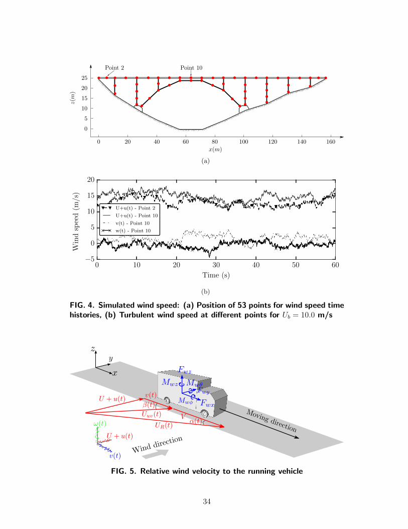
bridge and vehicle, the time histories of turbulent wind components in 53 points200
(see Fig. 4) are generated. For this generation of time histories, the value of201
the basic wind speed Ub is firstly proposed, and the mean wind speed at each202
point are then calculated according to its height. The main data of simulating203
conditions are adopted as follows:204
• Integral length scale: Lu = 100 m, Lv = 0.25Lu and Lω = 0.10Lu (Strømmen205
2006)206
• Turbulent intensities: Iu(z) = 1/ ln(z/z0), Iv = 0.75Iu and Iω = 0.50Iu207
9

(Strømmen 2006)208
• Upper cutoff frequency: fup = 12.0 Hz209
• Dividing number of frequency: Nf = 1024210
• Time interval: dt = 0.002 s211
A range of the basic wind velocity from 5.0 to 30.0 m/s in increments of212
0.5 m/s has been considered to study the influence of the crosswind velocity,213
Figure 4(b) shows the time histories of the longitudinal component of turbulent214
crosswind velocity at the two points indicated in figure 4(a) for Ub = 10.0 m/s.215
WIND-VEHICLE-BRIDGE INTERACTION216
The coupled vehicle-bridge system under turbulent crosswind is governed by217
a complicated dynamic interaction problem that involves interaction between the218
wind and the vehicle, the wind and the bridge, and the vehicle and the bridge.219
The interaction wind-vehicle and wind-bridge interaction is modelled through the220
aerodynamic forces applied to the vehicle and the bridge. A detailed description221
on how to obtain these aerodynamic forces is given in the next section. On the222
other hand, the vehicle-bridge interaction is established between the tires and223
the deck surface. In this study, a perfectly guided path is considered for the224
tire-deck surface interaction model, i.e. contact points between the tires and the225
deck surface share the position and velocity. In order to develop this tire-deck226
interaction model in Abaqus, a “node to surface” contact formulation (SIMULIA227
2011) is used between the bottom node of the tire elements and the deck surface.228
The augmented Lagrange method is applied then for the kinematic relations229
to enforce the corresponding contact constraints. Using augmented Lagrange230
formulation, the force vector applied on the vehicle and the bridge systems due231
to the interaction can be determined as:232
10

FCv
FCb
= ∇ΦTΛ +∇ΦTΥΦ (5)
where∇ΦT = ∂Φ/∂x; x = [xv,xb] is the global vector of displacement unknowns,233
Φ is the constraints vector that links the bottom node of the tire elements with the234
deck surface; Λ and Υ are the Lagrange multiplier vector and the penalty matrix235
of the coupled system, respectively; Fcv is force vector applied on the vehicle as236
consequence of the interaction with structure, and FCb their counterparts on the237
structure.238
The proposed methodology is developed in Abaqus (SIMULIA 2011), which239
allows to model the bridge structure by means of finite elements and the vehicle240
using multibody systems. The multibody dynamic equilibrium equations include241
second order and nonlinear terms related to the inertial forces (gyroscopic, cori-242
olis, centrifugal) that, in addition to the inherent nonlinearity introduced by the243
moving contact in the wheels, leads to a nonlinear coupled system of equations244
that defines the wind-vehicle-bridge interaction problem. This system can be245
expressed in the following matrix form, including the interaction forces and aero-246
dynamic forces:247
Mv 0
0 Mb
xv
xb
+
Cv 0
0 Cb
xv
xb
+
Kv 0
0 Kb
xv
xb
=
Fwv
Fwb
+
FCv
FCb
(6)
where Fwv , Fw
b is the aerodynamic wind force vector applied on the vehicle and248
bridge, respectively; Mv, Cv, Kv are the mass, damping and stiffness matrix of249
the vehicle, respectively; Mb, Cb, Kb are the mass, damping and stiffness matrix250
of the bridge, respectively.251
11

The HHT-α implicit integration method (Hilber et al. 1977) is used to solve252
the system of differential equations (6) in the time domain. A constant time step253
of 0.001 s is adopted, which is small enough to accurately capture high frequency254
vibrations and to account for the contribution of high-order spatial frequencies255
of the roughness profile.256
WIND-INDUCED EFFECTS257
Wind forces on the vehicle258
The aerodynamics forces and moments acting on the running vehicle under259
crosswind are represented in Fig. 5. These are determined using the quasi-static260
approach according to (Snæ bjornsson et al. 2007). Assuming that the mean261
wind velocity U is perpendicular to the longitudinal axis of the bridge deck (the262
x axis) and the vehicle runs over the bridge with a constant speed V the relative263
wind velocity UR and the angle of incidence α (see Fig. 5) can be determined at264
each instant t as follows:265
UR(t) =√
(U + u(t))2 + (v(t) + V )2 (7)
α(t) = arctan
(U + u(t)
v(t) + V
)(8)
where u(t) and v(t) are the longitudinal and horizontal components of turbulent266
crosswind, respectively. It should be noted that the wind time-history applied on267
the running vehicle is different from that applied on the surrounding nodes of the268
deck, from which it is linearly interpolated maintaining the compatibility.269
Wind forces on the bridge270
Based on the buffeting theory, the wind induced forces on the bridge structure271
can be determined from the instantaneous velocity pressure and the loads coeffi-272
12

cients. The wind-induced forces per unit length on the bridge may be expressed273
in vector form as follows (Strømmen 2006):274
FD(x, t)
FL(x, t)
Mx(x, t)
=1
2ρU2
R
DCD(αe)
BCL(αe)
B2CM(αe)
(9)
where UR is the instantaneous relative wind velocity, CD(αe), CL(αe), CM(αe)275
are drag, lift and moment aerodynamic coefficients that are functions of the angle276
of wind incidence αe (see Fig. 6), D and B are height and width of deck bridge277
section. In structural axis, the equation (9) is transformed into:278
Fwb (x, t) =
Fy
Fz
Mx
=
cos β − sin β 0
sin β cos β 0
0 0 1
FD
FL
Mx
(10)
The formulation using the Scalan’s frequency dependent flutter derivatives279
(Scanlan and Tomko 1971) is usually used in the modal frequency domain. How-280
ever, in this study the dynamic calculation is performed in the direct time domain,281
therefore, the aerodynamic forces can be decomposed, using the linearization ap-282
proach, as follows (Strømmen 2006):283
Fwb = Fs︸︷︷︸
static
+ B · v︸ ︷︷ ︸aerodynamic
+ Cae · r + Kae · r︸ ︷︷ ︸aeroelastic
(11)
where Fs, B·v and Cae·r+Kae·r represent the static, aerodynamic and aeroelastic284
13

effects, respectively, and are defined as:285
Fs =1
2ρU2B
(D/B)CD
CL
BCM
∣∣∣∣∣∣∣∣∣∣αs
(12a)
B =1
2ρUB
2(D/B)CD (D/B)C ′D − CL
2CL C ′L + (D/B)CD
2BCM BC ′M
∣∣∣∣∣∣∣∣∣∣αs
(12b)
Cae = −1
2ρUB
2(D/B)CD (D/B)C ′D − CL 0
2CL C ′L + (D/B)CD 0
2BCM BC ′M 0
∣∣∣∣∣∣∣∣∣∣αs
(12c)
Kae =1
2ρU2B
0 0 (D/B)C ′D
0 0 C ′l
0 0 BC ′M
∣∣∣∣∣∣∣∣∣∣αs
(12d)
v =
[u w
]T(12e)
r =
[p h α
]T(12f)
in which αs is the angle of attack of the wind respect to the position of the bridge286
elements (deck, arch, piers) at the static equilibrium position. p, h, α are the287
horizontal, vertical and torsional displacement of the structure under turbulent288
wind (see Fig. 6). The prime symbol in C ′D, C′L, C
′M indicates derivation of the289
aerodynamic coefficients with respect to the angle of attack. These derivatives290
are obtained from the computational fluid dynamic analysis of the deck, arch291
and piers (see Appendix III). It can be seen that the static and aerodynamic292
parts are functions of the mean wind (U) and its turbulence (u and w), while293
14

the aeroelastic part is associated with the structural velocity and displacement.294
The static and aerodynamic parts can be introduced into the structural elements295
via nodal forces in Abaqus software. However, due to the structural motion296
dependence of the aeroelastic part there is no direct way to introduce these forces297
in Abaqus software. In order to model the aeroelastic wind forces an user element298
has been developed within Abaqus using user subroutine UEL (SIMULIA 2011).299
The basic idea used here is that the user element is attached to each node of the300
structural bridge element as shown in Fig. 7. The user element will provide to301
the model during the transient analysis steps the forces Fi at the node i that302
depend on the values of the degrees of freedom Xbi at this node (each structural303
bridge element has six degrees of freedom).304
It is noted that the forces Fi generated by user element must be the same305
aeroelastic wind forces acting on this node, therefore, the nodal forces Fi can be306
expressed as307
Fi = Caei Xb
i + Kaei Xb
i (13)
where Kaei and Cae
i represent the local aeroelastic stiffness and damping matrices308
at the node i, respectively. From the equations (12d) and (12e), the expressions309
15

of Kaei and Cae
i can be determined as following310
Kaei =
1
2ρU2Blwi
0 0 0 0 0 0
0 0 0 (D/B)C ′D 0 0
0 0 0 C ′L 0 0
0 0 0 BC ′M 0 0
0 0 0 0 0 0
0 0 0 0 0 0
∣∣∣∣∣∣∣∣∣∣∣∣∣∣∣∣∣∣∣∣αs
(14a)
Caei = −1
2ρUBlwi
0 0 0 0 0 0
0 2(D/B)CD (D/B)C ′D − CL 0 0 0
0 2CL C ′L + (D/B)CD 0 0 0
0 2BCM BC ′M 0 0 0
0 0 0 0 0 0
0 0 0 0 0 0
∣∣∣∣∣∣∣∣∣∣∣∣∣∣∣∣∣∣∣∣αs
(14b)
where lwi is the length along which the wind forces acting on the structural311
element are lumped to the node i. The above definition of the UEL is presented312
with generality and it is readily applicable to any FE software. Further details on313
the specified implementation of this UEL to Abaqus are described in Appendix314
II. Using this methodology, the wind induced forces are applied to all the bridge315
elements, including the deck, the arch and the piers.316
RESULTS AND DISCUSSION317
The deck of the Wild bridge has been designed to support two road lanes and318
one sidewalk as shown in Fig. 8. With this design, the road axis is eccentric319
0.35 m with respect to the bridge axis which implies that the vehicles run over320
the bridge with certain eccentricity. In the previous work (Nguyen et al. 2015),321
16

it’s observed that the larger the vibration at the sidewalk is obtained when the322
passing vehicle is transversely closer to the sidewalk. Therefore, the load case in323
which the vehicle runs on the lane 1 with eccentricity of 1.4 m is selected for this324
study (see Fig. 8). To eliminate the possible effect generated due to the suddenly325
applied aerodynamic wind forces on the dynamic response of the vehicle and to326
study the possible effect generated during the time that the vehicle enters and327
leaves the bridge, the external platforms with roughness surface are considered328
at both abutments of the bridge in all calculations.329
As mentioned in section 4, in order to study the influence of the crosswind330
different levels of the basic wind velocity are used. In fact, a range from 5.0 to331
30.0 m/s in increment of 0.5 m/s has been considered. Furthermore, for each332
level of basic wind velocity, a range of vehicle velocities ranging from 60 to 120333
km/h, in increments of 10 km/h, is considered to investigate the ride comfort and334
safety of the road vehicle. An extensive number of analyses are performed and335
the main obtained results are presented and discussed below.336
Effects of crosswind on the bridge vibration337
In order to assess effects of the turbulent crosswind on the bridge vibration, the338
time histories of vertical and lateral acceleration of all points along the sidewalk339
are recorded in all calculations. The maximum acceleration at each point is then340
determined. Fig. 9(a) shows the peak vertical acceleration along the sidewalk341
for different levels of the basic wind velocity when the vehicle crosses the bridge342
at v = 100 km/h. The result without crosswind is also included for comparison.343
It can be observed that for gentle crosswind (Ub = 5 m/s) the vibration of deck344
is similar to the case without crosswind. It can be due to that the aerodynamic345
wind forces are too low to produce any meaningful inertia effects, comparing with346
the forces generated by the passing vehicle. But, as the crosswind is stronger and347
17

more moderate, the vibration of deck is larger. Furthermore, it is seen that the348
zone of arch span is the one more affected by the crosswind as expected, since349
the wind velocity in this zone is higher. In fact, if the basic wind velocity is of350
25.0 m/s, the maximum vertical acceleration obtained at point C1 can be up to351
10.5 times higher than the case without crosswind and 1.5 times higher than the352
maximum acceleration allowed (alim = 0.5√f0 = 0.81 m/s2) by some codes (BS353
5400-2:2006 2006; RPX-95 1995) for deck vibration. Moreover, from Fig. 9(a)354
the impact effect can be observed when the vehicle enters and leaves the bridge.355
Such peak acceleration at the deck nearby the abutments would far exceed the356
admissible limit in SLS of vibration (alim). The human response to vibration357
depends, of course, on the level or magnitude of vibration, but also depends on358
the other important factors such as frequency content of the vibration, exposure359
time, direction of application, etc. Further analysis have been done in order to360
evaluate the human comfort. The RMS acceleration in one-third octave frequency361
bands are obtained from the acceleration time histories. These RMS acceleration362
are then compared with the vertical base curve for acceptable human response363
under storm conditions proposed by Irwin (Irwin 1978). A representative result364
is shown in Fig. 9(b), in which the vertical RMS accelerations at the point C1365
are represented for different levels of the basic wind velocity. The result in Fig.366
9(b) reaffirms the important influence of crosswind on the vertical vibration of367
this bridge and the need for considering the aerodynamic actions introduced by368
wind in the general vibration assessment of bridges. Additionally, it can be seen369
that the RMS accelerations will exceed the limit comfort curve considering the370
threshold for frequent events when the wind is strong (25.0 m/s), which means371
that the human, in this case, pedestrian users feel or sense discomfort due to the372
bridge vibration.373
Respect to the lateral vibration of the bridge, the same results are represented374
18

in Fig. 10. The peak lateral accelerations along the sidewalk are obtained and375
plotted for different levels of the basic wind velocity (Ub), and compared with376
the limit of comfort established by IAP-11 (IAP-11 2011) (alim = 0.8 m/s2) (see377
Fig. 10(a)). The RMS accelerations in one-third octave frequency bands at378
the point C1 are also plotted and compared with the lateral acceleration base379
curve for acceptable human response proposed by Irwin (Irwin 1978). Figure380
10(a) shows that the peak lateral acceleration on the deck is only increased by381
the crosswind on the sections corresponding to the arch due to the increased382
transverse flexibility of the bridge in this area. Furthermore, this effect is only383
appreciable for relatively strong wind speeds, which is attributed to important384
slenderness of the deck and the reduced aerodynamic forces. However, from Fig.385
10(b) it can be noted that the crosswind has an important effect on the frequency386
content of the acceleration signals of this structure, specially in the range [0.4−10]387
Hz. The RMS acceleration in one-third octave bands at point C1 increases with388
the wind velocity, and it nearly reaches the limit curve for Ub = 25.0 m/s. This389
demonstrates that, as expected, the pedestrians comfort decreased by increasing390
the lateral wind speed and it can only be tackled by using criteria that account391
for the excitation frequency, such as Iwin’s392
In order to explore the participation of the wind- and traffic-induced vibration393
on the frequency content of the response of the deck, the time histories of the deck394
acceleration is analyzed in the frequency domain. Fig. 11 shows the frequency395
content of the vertical and lateral acceleration at point C1 when the vehicle crosses396
over the bridge at V = 100 km/h, for different basic wind speeds. It can be397
observed from Fig. 11(a) that three modes dominate the vertical deck vibration.398
The dominance of the first vertical mode is observed, specially for strong winds399
(Ub = 25.0 m/s), but it is also apparent the important participation of the third400
vertical mode (approximately 5 Hz) and the torsional mode (in the range of 10401
19

Hz). This result directly questions the applicability of extended comfort criteria402
that are based on the assumption that the structure is completely dominated403
by a fundamental mode of vibration (BS 5400-2:2006 2006; RPX-95 1995). In404
comparison to the vertical vibration of the deck, the lateral vibration (Fig. 11(b))405
is more dominated by the first lateral mode for wind velocities below 20 m/s,406
beyond this value a group of closely spaced high-order mode between 5 and 10407
Hz increases significantly the response as shown in Fig. 11(b).408
Effects of crosswind on the road vehicle vibration409
In this section, the ride comfort and safety of road vehicle are addressed410
through the accelerations at the driver seat (see Fig. 3), the contact forces be-411
tween the tire and road. The weighted RMS acceleration and the RMS acceler-412
ation in one-third octave frequency bands are obtained from the time histories413
of the vertical and lateral acceleration at the driver’s seat in order to evalu-414
ate the vehicle users’ comfort. The resulting accelerations are compared with415
the indicative ranges of comfort given by ISO 2631 (ISO 2631-1:1997 1997) and416
fatigue-decreased proficiency boundaries proposed by ISO 2631 (ISO 2631:1978417
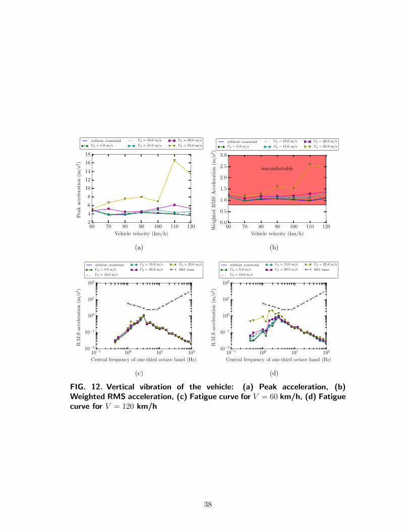
1978), respectively. Figure 12 shows the results for the vertical vibration of the418
vehicle. It can be observed that the maximum acceleration at driver’s seat is419
hardly affected by crosswinds below ranging from 5 to 20 m/s (see Fig. 12(a)),420
which is also noticed for the the weighted RMS accelerations (see Fig. 12(b)).421
Furthermore, there are high increments of acceleration for strong wind (Ub = 25.0422
m/s) compared with the other lower wind velocities. This is due to the fact that423
the strong wind increases the vehicle vibration on the one hand, and increases424
the bridge vibration on the other which also influences the vehicle vibration, as425
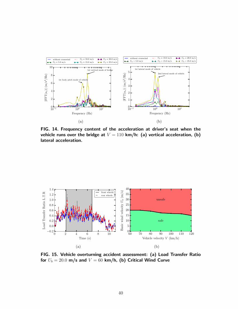
shown in Fig. 14(a). Interestingly, all recorded values of RMS accelerations in426
the vehicle are regarded as “uncomfortable” according to ISO’s criterion (ISO427
20
2631-1:1997 1997), including the case in which the wind is not considered and for428
all the vehicle velocities considered. The validity of the comfort criteria for the429
vertical vibrations in the vehicle considered should be questioned based on these430
results. Firstly, it is noted that the scope of this work is the global assessment of431
the user’s comfort and safety due to the wind-vehicle-bridge interaction, and no432
attempt was made to simulate the filtering effect of the vehicle seat or other local433
effects in the vehicle. Secondly, the indicative comfort range proposed by ISO434
2631 (ISO 2631-1:1997 1997) gives approximate indications of likely reactions to435
various magnitudes of overall vibration total values in public transport, and ISO436
2631 does not define any limit for acceptable values of magnitude for comfort.437
From Fig. 12(c) and 12(d), it can be seen that the crosswind hardly effect on the438
vertical ride comfort of vehicle.439
Fig. 13 shows the results of the lateral vibration of vehicle. It is observed440
that the crosswind influences significantly the lateral acceleration in the vehicle441
and the comfort of its user regarding vibrations in this direction. Indeed, the442
peak acceleration and the weighted RMS acceleration increase by increasing the443
crosswind velocity. The RMS accelerations in the one-third octave bands are444
also larger when the crosswind speed increases. The RMS accelerations almost445
reach the limit curve for fatigue-decreased proficiency when the velocity of the446
vehicle is 120 km/h and the crosswind speed is 25.0 m/s, indicating that the447
driver could feel fatigue and decrease his proficiency to drive. In contrast to448
the vertical vibration of the vehicle, its lateral vibration is not influenced by the449
bridge vibration, but is only influenced by its lateral vibration modes, as shown450
in Fig. 14(b).451
Vehicle accidents can be categorized in three main types: overturning, side-452
slipping and yawing (rotational) accidents (Baker and Reynolds 1992). Side-453
slipping accidents and yawing may occur if the coefficient of friction between the454
21

tires and the road surface is low (Snæ bjornsson et al. 2007; Zhou and Chen 2015)455
(e.g. in wet pavements). However, the assessment of side-slipping and, especially,456
yawing accidents, requires detailed information about the contact between the457
tires and the pavement, as well as the model of the driver’s response (Chen and458
Cai 2004). This work will focus only on vehicle overturnings because it represents459
the most common type of wind-induced vehicle accidents (Baker and Reynolds460
1992). It should be noted, however, that the methodology presented in this paper461
is applicable to the study of the other types of accidents.462
An overturning accident occurs when one of the tire reactions is zero, in other463
words, the vertical load is transferred from the tires on the windward side of the464
vehicle to those on the leeward side. The Load Transfer Ratio (LTR) is employed465
to quantify the load transference and is defined as:466
LTR =FL − FRFL + FR
(15)
where FL and FR are the vertical tire reactions on the left (leeward) and right467
(windward) sides, respectively. The LTR is 0.0 when the loads on two sides468
are equal and ±1.0 when all the load is transferred to the leeward side and the469
vehicle is on the verge of an overturning accident. The LTR of the front and rear470
wheels are plotted in Fig. 15(a) for a certain vehicle and wind velocity. It can471
be observed that the load transfer reaches larger value when the vehicle is at the472
arch span, as expected. This is because that the crosswind velocity in this section473
of the bridge is higher than those of other sections of the bridge. The LTR at474
the rear wheel is higher than at the front wheel, as expected. It is due to that475
the rear wheels have less gravity load from the carbody by the position of gravity476
centre, and therefore these wheels govern the overturning accident.477
Based on the LTR, the critical wind speed can be determined for each vehicle478
22

velocity when at this speed the vehicle overturns. Consequently, the critical wind479
curve (CWC) can be obtained from the all critical wind speed for the whole range480
of the vehicle velocities. Figure 15(b) represents the CWC obtained in this work481
for the bridge. Assuming a vehicle velocity limit of 120 km/h, it is observed that482
no restriction should be imposed when the wind speed is below 15 m/s, which483
could be considered as the critical wind speed for this bridge.484
CONCLUSIONS485
In this paper, the dynamic effects of turbulent crosswind on the serviceability486
state of vibrations and the vehicle accident risk are addressed in a slender arch487
by means of the wind-vehicle-bridge interaction analyses. A new finite element is488
developed for the application of aerodynamic wind actions in general Finite Ele-489
ment Analysis software packages. This element is able to provide the aeroelastic490
wind forces. The results of the fully coupled nonlinear dynamic analysis drawn491
the following conclusions on the dynamic response of the studied bridge:492
• The bridge vibration is significantly affected by the crosswind in terms493
of the peak acceleration and the frequency content when the crosswind is494
moderate and strong (Ub > 15 m/s). However, for lower wind speeds (below495
10 m/S) the deck vibration is governed by the passing vehicle.496
• The criteria for the SLS of vertical vibration based on the peak acceleration497
is easily exceeded at almost point of the deck when the crosswind is strong498
(Ub = 25.0 m/s). Analyzing in the frequency domain the vibration level is499
still below the limit comfort curve, and therefore, is comfortable. Further-500
more, the vertical bridge vibration is significantly influenced by high-order501
vibration modes between 5 and 10 Hz that would be ignored according to502
code-based comfort criteria such as (BS 5400-2:2006 2006; RPX-95 1995).503
23
• Previous research works observed the importance of the road roughness504
surface on the ride comfort of the vehicle. In this study, it is observed that it505
also depends on the vehicle velocity and the crosswind speed. It is observed506
that the crosswind has more effect on ride comfort of the vehicle in lateral507
direction than in the vertical direction. When the vehicle runs over the508
bridge with the velocity of 120 km/s and with a strong crosswind velocity509
(Ub = 25.0 m/s), the driver could experience the fatigue and decrease his510
proficiency to drive.511
• For the “good” road surface quality considered in this study, the basic wind512
speed of 15 m/s could be considered as the critical speed in the studied513
bridge for the circulation.514
ACKNOWLEDGEMENTS515
The authors thank to other members of the team of Intitut fur Betonbau at516
Technical University of Graz: Berhard Freytag, Michael Reichel, who provided517
the necessary information of the Wild bridge design. K.Nguyen and O. Rio also518
thank to the MINECO of Spain for the support of the project BIA2013-48480-519
C2-1R.520
REFERENCES521
American Association of State Highway and Transportation Officials (1998).522
AASHTO LRFD: Bridge design specifications. Washington, EE UU.523
Azizinamini, A., Barth, K., Dexter, R., and Rubeiz, C. (2004). “High Performance524
Steel: Research FrontHistorical Account of Research Activities.” Journal of525
Bridge Engineering, 9(3), 212–217.526
Baker, C. J. and Reynolds, S. (1992). “Wind-induced accidents of road vehicles.”527
Accident Analysis and Prevention, 24(6), 559–575.528
24

Boggs, D. and Petersen, C. P. (1995). “Acceleration indexes for human comfort529
in tall buildings - peak or rms?530
BS 5400-2:2006 (2006). Steel, concrete and composite bridges - Part 2: Specifica-531
tion for loads. British Standard, UK.532
BS 6841:1987 (2012). Guide to measurement and evaluation of human exposure533
to whole-body mechanical vibration and repeated shock.534
Cai, C. and Chen, S. (2004). “Framework of vehiclebridgewind dynamic analysis.”535
Journal of Wind Engineering and Industrial Aerodynamics, 92(7-8), 579–607.536
Camara, A., Nguyen, K., Ruiz-Teran, A., and Stafford, P. (2014). “Serviceabil-537
ity limit state of vibrations in under-deck cable-stayed bridges accounting for538
vehicle-structure interaction.” Engineering Structures, 61, 61–72.539
CEN (2005a). EN 1337-3:2005 Structural bearings. Part 3: Elastomeric bearings.540
rue de Stassart, 36B-1050 Brussels.541
CEN (2005b). EN 1991-1-4: Actions on structures - Part 1-4: General actions -542
Wind actions. rue de Stassart, 36B-1050 Brussels.543
Chen, S. R. and Cai, C. S. (2004). “Accident assessment of vehicles on long-span544
bridges in windy environments.” Journal of Wind Engineering and Industrial545
Aerodynamics, 92(12), 991–1024.546
Chen, X., Matsumoto, M., and Kareem, A. (2000). “Time Domain Flutter and547
Buffeting Response Analysis of Bridges.” Journal of Engineering Mechanics,548
126(1), 7–16.549
Davenport, A. (1962). “Buffeting of a Suspension Bridge by Storm Winds.” Jour-550
nal of the Structural Division, 88(3), 233–270.551
Dodds, C. and Robson, J. (1973). “The description of road surface roughness.”552
Journal of Sound and Vibration, 31(2), 175–183.553
Griffin, M. J. (1990). Handbook of Human Vibration. Academic Press Inc. (Lon-554
don) Limited.555
25

Guo, W. H. and Xu, Y. L. (2006). “Safety Analysis of Moving Road Vehicles on556
a Long Bridge under Crosswind.” Journal of Engineering Mechanics, 132(4),557
438–446.558
Hilber, H. M., Hughes, T. J., and Taylor, R. L. (1977). “Improved numerical559
dissipation for time integration algorithms in structural dynamics.” Earthquake560
Engineering and Structural Dynamics, 5, 283–292.561
IAP-11 (2011). IAP-11: Instruccion sobre las acciones a considerar en el proyecto562
de puentes de carretera (in Spanish).563
Irwin, A. W. (1978). “Human response to dynamic motion of structures.” The564
Structural Engineer, 56A(9), 237–244.565
ISO 2631-1:1997 (1997). Mechanical vibration and shock – Evaluation of human566
exposure to whole-body vibration – Part 1: General requirements. International567
Organization for Standardization, Gineva.568
ISO 2631:1978 (1978). Guide for the evaluation of human exposure to whole-body569
vibration. International Organization for Standardization, Gineva.570
ISO 8608:1995 (1995). Mechanical vibration - Road surface profiles - Reporting of571
measured data. International Organization for Standardization (ISO), Gineva.572
JCSS (2001a). Probabilistic Model Code - Part 2: Load Models.573
JCSS (2001b). Probabilistic Model Code - Part 3: Material Properties.574
Kamash, K. M. A. and Robson, J. D. (1978). “The Application of Isotropy in575
Road Surface Modelling.” Journal of Sound and Vibration, 57(1), 89–100.576
Kuhne, M. and Orgass, M. (2009). “Prufbericht PB 1.1/09-126-4 : Uberwachung577
und Prufung von UHFRC fur das Bauvorhaben, Wild-Brucke.” Report no.,578
MFPA Leipzig GmbH.579
Miyata, T. and Yamada, H. (1990). “Coupled flutter estimate of a suspension580
bridge.” Journal of Wind Engineering and Industrial Aerodynamics, 33, 341–581
348.582
26

Moghimi, H. and Ronagh, H. R. (2008). “Development of a numerical model583
for bridgevehicle interaction and human response to traffic-induced vibration.”584
Engineering Structures, 30(12), 3808–3819.585
Nguyen, K., Freytag, B., Ralbovsky, M., and Rio, O. (2015). “Assessment of586
serviceability limit state of vibrations in the UHPFRC-Wild bridge through an587
updated FEM using vehicle-bridge interaction.” Computers & Structures, 156,588
29–41.589
Roeder, C. W., Barth, K. E., and Bergman, A. (2004). “Effect of Live-Load590
Deflections on Steel Bridge Performance.” Journal of Bridge Engineering, 9(3),591
259–267.592
RPX-95 (1995). RPX-95: Recommendations for the project of composite road593
bridges (in Spanish). Spain.594
Sayers, M. W. (1988). “Dynamic Terrain Inputs to Predict Structural Integrity of595
Ground Vehicles.” Report No. UMTRI-88-16, University of Michigan, Trans-596
portation Research Institute, Michigan.597
Scanlan, R. (1978). “The action of flexible bridges under wind, II: Buffeting598
theory.” Journal of Sound and Vibration, 60(2), 201–211.599
Scanlan, R. and Tomko, A. (1971). “Airfoil and Bridge Deck Flutter Derivatives.”600
Journal of the Engineering Mechanics Division, 97(6), 1717–1737.601
SIMULIA (2011). Abaqus Analysis User’s Manual, v6.11. Dassalt Systemes602
SIMULIA Corp.603
Snæ bjornsson, J. T., Baker, C. J., and Sigbjornsson, R. (2007). “Probabilistic604
assessment of road vehicle safety in windy environments.” Journal of Wind605
Engineering and Industrial Aerodynamics, 95(9-11), 1445–1462.606
Sparowitz, L., Freytag, B., Reichel, M., and Zimmermann, W. (2011). “Wild607
Bridge - A Sustainable Arch Made of UHPFRC.” 3rd Chinese - Croatian Joint608
Colloquium: Sustainable Arch Bridges, Zagreb, Croatia, 45–70.609
27

Sterling, M., Quinn, A. D., Hargreaves, D. M., Cheli, F., Sabbioni, E., Tomasini,610
G., Delaunay, D., Baker, C. J., and Morvan, H. (2010). “A comparison of611
different methods to evaluate the wind induced forces on a high sided lorry.”612
Journal of Wind Engineering and Industrial Aerodynamics, 98(1), 10–20.613
Strømmen, E. (2006). Theory of Bridge Aerodynamics. Springer.614
Veers, P. S. (1988). “Three-dimensional wind simulation.” SANDIA report,615
SAND88-0152 UC-261, Sandia National Laboratories, California, USA.616
Weller, H. G., Tabor, G., Jasak, H., and Fureby, C. (1998). “A tensorial ap-617
proach to computational continuum mechanics using object-oriented tech-618
niques.” Computers in Physics, 12(6), 620–631.619
Wright, R. N. and Walker, W. H. (2004). “Criteria for deflection of steel bridges.”620
Bulletin for the America Iron and Steel Institute, 19.621
Xu, Y. and Guo, W. (2004). “Effects of bridge motion and crosswind on ride622
comfort of road vehicles.” Journal of Wind Engineering and Industrial Aero-623
dynamics, 92(7-8), 641–662.624
Xu, Y. L. and Guo, W. H. (2003). “Dynamic analysis of coupled road vehicle and625
cable-stayed bridge systems under turbulent wind.” Engineering Structures, 25,626
473–486.627
Xu, Y. L., Sun, D. K., Ko, J. M., and Lin, J. H. (2000). “Fully coupled buffeting628
analysis of Tsing Ma suspension bridge.” Journal of Wind Engineering and629
Industrial Aerodynamics, 85(1), 97–117.630
Zhou, Y. and Chen, S. (2015). “Fully coupled driving safety analysis of moving631
traffic on long-span bridges subjected to crosswind.” Journal of Wind Engi-632
neering and Industrial Aerodynamics, 143, 1–18.633
APPENDIX I. PROPERTIES OF THE HIGH-SIDED TRUCK634
The main properties of the high-sided truck are listed in Table III.635
28

APPENDIX II. IMPLEMENTATION OF USER ELEMENT636
The user element is composed by 2 nodes. Each node has six degrees of637
freedom. In order to implement this element into the Abaqus software, there638
are two essential outputs that are required to be updated in the UEL subroutine639
(SIMULIA 2011). In particular, the residual quantity RHS := F and the element640
Jacobian AMATRX := −∂F/∂u must be updated in every interaction. The641
program Abaqus uses an implicit time integration and a full Newton solution642
technique to solve the static and dynamic problem. In the static analysis, the643
user element implemented here does not contribute any stiffness to the model,644
while this element will provide the nodal forces to the model in the dynamic645
analysis. The nodal forces depend on the values of the degrees of freedom of the646
nodes and according to (13) the nodal forces provided by the element is expressed647
as648
G = Cu + Ku (16)
where649
C =
Caei 0
0 Caei
and K =
Kaei 0
0 Kaei
(17)
According to (SIMULIA 2011), for the integration dynamic analysis the residual650
quantity and the element Jacobian at time t+∆t must be determined as following651
RHS = F = −Mut+∆t + (1 + α)Gt+∆t − αGt (18a)
AMATRX = M(du/du) + (1 + α)C(du/du) + (1 + α)K (18b)
29

where MNM is the mass matrix of the user element (for the implemented element,652
MNM = [0]), α is the factor for numerical damping used in HHT method. The653
values of the nodal forces are recorded as solution-dependent state variables for654
each time increment in order to determine RHS as defined in equation (18a).655
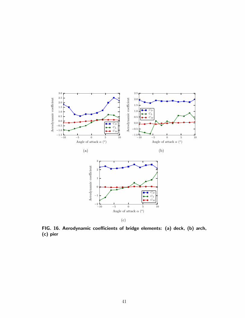
APPENDIX III. AERODYNAMIC PROPERTIES OF BRIDGE656
The aerodynamic coefficients and their derivatives are obtained from two di-657
mensional Computational Fluid Dynamic analysis of the deck, arch and pier658
sections using OpenFOAM v.2.3 (Weller et al. 1998). The turbulence model fol-659
lows the Reynolds Average Simulation (RAS) technique. The Reynolds number660
in the analyses is in the order of 107. Care was taken on the selection of the mesh661
size. After a sensitivity analysis the element size in the vicinity of the obstacles662
is selected as 3 mm.663
30

List of figures664
1 10 100 1 10 100
Longitudinal (z-axis) Vibration Transverse (x-axis and y-axis) Vibration
0.1
1.0
10
100
1 Minute
Exposures
24 Hour
Exposures
1 Minute
Exposures
24 Hour
Exposures
Exposure limit
Fatigue-decreased
proficiency boundary
Reduced comfort
boundary
0.1
1.0
10
100
0.01 0.01
Accele
ration (
m/s
2r.
m.s
)
Frequency (Hz)
FIG. 1. Exposure limits, fatigue-decreased proficiency boundaries and re-duced comfort boundaries to whole-body vibrations given in ISO 2631:1978(adapted from Handbook of Human Vibration, M. J. Griffin (Griffin 1990),Chapter 10 “Whole-body Vibration Standards”, 415–451, Copyright 1990,with permission from Elsevier)
31

(a)
(b) (c)
FIG. 2. Wild Bridge: (a) general view (image by L. Sparowitz), (b) crosssection, (c) knee node
32

(a) (b)
FIG. 3. High-sided vehicle model in dynamic analysis: (a) side view, (b)front view
33
(a)
0 10 20 30 40 50 60
Time (s)
−5
0
5
10
15
20
Windspeed(m
/s)
U+u(t) - Point 2
U+u(t) - Point 10
v(t) - Point 10
w(t) - Point 10
(b)
FIG. 4. Simulated wind speed: (a) Position of 53 points for wind speed timehistories, (b) Turbulent wind speed at different points for Ub = 10.0 m/s
FIG. 5. Relative wind velocity to the running vehicle
34

FIG. 6. Diagram of turbulent crosswind actuating on bridge elements
FIG. 7. User element for modelling the aeroelastic wind forces
(a) (b)
FIG. 8. Load case considered in this study: (a) cross section, (b) plan viewand elevation of the bridge, including some control points employed to referthe ongoing results
35

0 20 40 60 80 100 120 140
Distance; X (m)
0.0
0.5
1.0
1.5
2.0
2.5
Peakacceleration
(m/s
2)
without crosswind
Ub = 5.0 m/s
Ub = 10.0 m/s
Ub = 15.0 m/s
Ub = 20.0 m/s
Ub = 25.0 m/s
alim
(a)
10−1 100 101 102
Central frequency of one-third octave band (Hz)
10−4
10−3
10−2
10−1
100
101
102
RMSacceleration
(m/s
2)
without crosswind
Ub = 5.0 m/s
Ub = 10.0 m/s
Ub = 15.0 m/s
Ub = 20.0 m/s
Ub = 25.0 m/s
Irwin (storm cond.)
Irwin (freq. events)
(b)
FIG. 9. Effects of crosswind on the vertical vibration of the bridge at v=100km/h: (a) Peak acceleration along sidewalk, (b) RMS acceleration in one-third octave frequency bands at point C1
0 20 40 60 80 100 120 140
Distance; X (m)
0.0
0.1
0.2
0.3
0.4
0.5
0.6
0.7
0.8
0.9
Peakacceleration
(m/s
2)
without crosswind
Ub = 5.0 m/s
Ub = 10.0 m/s
Ub = 15.0 m/s
Ub = 20.0 m/s
Ub = 25.0 m/s
alim
(a)
10−1 100 101 102
Central frequency of one-third octave band (Hz)
10−5
10−4
10−3
10−2
10−1
100
101
RMSacceleration
(m/s
2)
without crosswind
Ub = 5.0 m/s
Ub = 10.0 m/s
Ub = 15.0 m/s
Ub = 20.0 m/s
Ub = 25.0 m/s
Irwin (storm cond.)
Irwin (freq. events)
(b)
FIG. 10. Effects of crosswind on the lateral vibration of the bridge at v=100km/h: (a) Peak acceleration along sidewalk, (b) RMS acceleration in one-third octave frequency bands at point C1.
36

100 101
Frequency (Hz)
0.0
0.1
0.2
0.3
0.4
0.5
|FFT(a
v)|(m
/s2/H
z)
1st vertical mode
3rd vertical mode
torsional mode
without crosswind
Ub = 5.0 m/s
Ub = 10.0 m/s
Ub = 15.0 m/s
Ub = 20.0 m/s
Ub = 25.0 m/s
(a)
10−1 100 101
Frequency (Hz)
0.00
0.01
0.02
0.03
0.04
0.05
0.06
0.07
|FFT(a
v)|(m
/s2/H
z)
1st lateral mode
without crosswind
Ub = 5.0 m/s
Ub = 10.0 m/s
Ub = 15.0 m/s
Ub = 20.0 m/s
Ub = 25.0 m/s
(b)
FIG. 11. Frequency content of deck acceleration at point C1 when the ve-hicle runs over the bridge at V = 100 km/h: (a) vertical acceleration, (b)lateral acceleration.
37
60 70 80 90 100 110 120
Vehicle velocity (km/h)
2
4
6
8
10
12
14
16
18
Peakacceleration
(m/s
2)
without crosswind
Ub = 5.0 m/s
Ub = 10.0 m/s
Ub = 15.0 m/s
Ub = 20.0 m/s
Ub = 25.0 m/s
(a)
60 70 80 90 100 110 120
Vehicle velocity (km/h)
0.0
0.5
1.0
1.5
2.0
2.5
3.0
Weigh
tedRMSAcceleration(m
/s2)
uncomfortable
without crosswind
Ub = 5.0 m/s
Ub = 10.0 m/s
Ub = 15.0 m/s
Ub = 20.0 m/s
Ub = 25.0 m/s
(b)
10−1 100 101 102
Central frequency of one-third octave band (Hz)
10−2
10−1
100
101
102
R.M
.Sacceleration
(m/s
2)
without crosswind
Ub = 5.0 m/s
Ub = 10.0 m/s
Ub = 15.0 m/s
Ub = 20.0 m/s
Ub = 25.0 m/s
ISO 1min
(c)
10−1 100 101 102
Central frequency of one-third octave band (Hz)
10−2
10−1
100
101
102
R.M
.Sacceleration
(m/s
2)
without crosswind
Ub = 5.0 m/s
Ub = 10.0 m/s
Ub = 15.0 m/s
Ub = 20.0 m/s
Ub = 25.0 m/s
ISO 1min
(d)
FIG. 12. Vertical vibration of the vehicle: (a) Peak acceleration, (b)Weighted RMS acceleration, (c) Fatigue curve for V = 60 km/h, (d) Fatiguecurve for V = 120 km/h
38

60 70 80 90 100 110 120
Vehicle velocity (km/h)
0
1
2
3
4
5
6
Peakacceleration
(m/s
2)
without crosswind
Ub = 5.0 m/s
Ub = 10.0 m/s
Ub = 15.0 m/s
Ub = 20.0 m/s
Ub = 25.0 m/s
(a)
60 70 80 90 100 110 120
Vehicle velocity (km/h)
0.0
0.5
1.0
1.5
2.0
2.5
Weigh
tedRMSAcceleration(m
/s2)
uncomfortable
without crosswind
Ub = 5.0 m/s
Ub = 10.0 m/s
Ub = 15.0 m/s
Ub = 20.0 m/s
Ub = 25.0 m/s
(b)
10−1 100 101 102
Central frequency of one-third octave band (Hz)
10−5
10−4
10−3
10−2
10−1
100
101
102
R.M
.Sacceleration
(m/s
2)
without crosswind
Ub = 5.0 m/s
Ub = 10.0 m/s
Ub = 15.0 m/s
Ub = 20.0 m/s
Ub = 25.0 m/s
ISO 1min
(c)
10−1 100 101 102
Central frequency of one-third octave band (Hz)
10−4
10−3
10−2
10−1
100
101
102
R.M
.Sacceleration
(m/s
2)
without crosswind
Ub = 5.0 m/s
Ub = 10.0 m/s
Ub = 15.0 m/s
Ub = 20.0 m/s
Ub = 25.0 m/s
ISO 1min
(d)
FIG. 13. Lateral vibration of the vehicle: (a) Peak acceleration, (b)Weighted RMS acceleration, (c) Fatigue curve for V = 60 km/h, (d) Fatiguecurve for V = 120 km/h
39
10−1 100 101
Frequency (Hz)
0
2
4
6
8
10
|FFT(a
v)|(m
/s2/H
z)
1st body pitch mode of vehicle
1st vertical mode of bridge
without crosswind
Ub = 5.0 m/s
Ub = 10.0 m/s
Ub = 15.0 m/s
Ub = 20.0 m/s
Ub = 25.0 m/s
(a)
10−1 100 101
Frequency (Hz)
0
1
2
3
4
5
|FFT(a
v)|(m
/s2/H
z)
1st lateral mode of vehicle
2nd lateral mode of vehicle
without crosswind
Ub = 5.0 m/s
Ub = 10.0 m/s
Ub = 15.0 m/s
Ub = 20.0 m/s
Ub = 25.0 m/s
(b)
FIG. 14. Frequency content of the acceleration at driver’s seat when thevehicle runs over the bridge at V = 110 km/h: (a) vertical acceleration, (b)lateral acceleration.
0 2 4 6 8 10
Time (s)
−0.2
0.0
0.2
0.4
0.6
0.8
1.0
1.2
1.4
LoadTransfer
Ratio
L.T.R
front wheels
rear wheels
(a)
60 70 80 90 100 110 120
Vehicle velocity V (km/h)
0
5
10
15
20
25
30
35
40
Basic
windvelocity
Ub(m
/s)
safe
unsafe
(b)
FIG. 15. Vehicle overturning accident assessment: (a) Load Transfer Ratiofor Ub = 20.0 m/s and V = 60 km/h, (b) Critical Wind Curve
40
−10 −5 0 5 10
Angle of attack α (o)
−1.5
−1.0
−0.5
0.0
0.5
1.0
1.5
2.0
2.5
3.0
Aerodynamic
coeffi
cient
CD
CL
CM
(a)
−10 −5 0 5 10
Angle of attack α (o)
−1.0
−0.5
0.0
0.5
1.0
1.5
2.0
2.5
Aerodynamic
coeffi
cient
CD
CL
CM
(b)
−10 −5 0 5 10
Angle of attack α (o)
−2
−1
0
1
2
3
Aerodynamic
coeffi
cient
CD
CL
CM
(c)
FIG. 16. Aerodynamic coefficients of bridge elements: (a) deck, (b) arch,(c) pier
41

TABLE 1. Main characterization of parameters of the numerical model ofWild bride
Notation Parameter UnitAdopted and/or
Referencesupdated value
Ea Elastic modulus of arches GPa 53.3 (Nguyen et al. 2015)ρa Mass density of arches kg/m3 2590 (JCSS 2001a; Kuhne and Orgass 2009)Ep Elastic modulus of bridge piers GPa 41.4 (Nguyen et al. 2015)ρp Mass density of bridge piers kg/m3 2500 (JCSS 2001a)Ed Elastic modulus of deck GPa 38.0 (Nguyen et al. 2015)ρd Mass density of deck kg/m3 2518.7 (Nguyen et al. 2015)md Nonstructural mass on deck kg/m2 216.0 (JCSS 2001a)hd Thickness of deck m 0.601 (Nguyen et al. 2015)Eeb Bulk modulus of the bearing GPa 834 (JCSS 2001b)
TABLE 2. Summary of first six modes of vibration of the bridge
Mode Frequency (Hz) Description1 0.874 1st lateral bending2 2.371 2nd lateral bending3 2.586 1st vertical bending4 2.895 2nd vertical bending5 3.971 3rd vertical bending6 4.607 3rd lateral bending
42

TABLE 3. Main parameters of the high-sided truck
Notation Parameter Valuemc Mass of truck body (kg) 4480Jcy Pitching moment of inertia of track body (kg.m2) 5516Jcx Rolling moment of inertia of track body (kg.m2) 1349Jcz Yawing moment of inertia of track body (kg.m2) 100000mr,i (i = 1, 2) Mass of rear axle set(kg) 710mf,i (i = 1, 2) Mass of front axle set(kg) 800kz,si (i = 1, 2, 3, 4) Vertical stiffness of suspension along Z axis (kN/m) 399ky,si (i = 1, 2, 3, 4) Lateral stiffness of suspension along Z axis (kN/m) 299cz,si (i = 1, 2) Vertical damping of rear suspension along Z axis (kN s/m) 5.18cy,si (i = 1, 2) Lateral damping of rear suspension along Z axis (kN s/m) 5.18cz,si (i = 3, 4) Vertical damping of front suspension along Z axis (kN s/m) 23.21cy,si (i = 3, 4) Lateral damping of front suspension along Z axis (kN s/m) 23.21kz,fi (i = 1, 2) Vertical stiffness of front tire (kN/m) 351kz,ri (i = 1, 2) Vertical stiffness of rear tire (kN/m) 351ky,fi (i = 1, 2) Lateral stiffness of front tire (kN/m) 121ky,ri (i = 1, 2) Lateral stiffness of rear tire (kN/m) 121cz,fi (i = 1, 2) Vertical damping of front tire (kN s/m) 0.80cz,ri (i = 1, 2) Vertical damping of rear tire (kN s/m) 0.80cy,fi (i = 1, 2) Lateral damping of front tire (kN s/m) 0.80cy,ri (i = 1, 2) Lateral damping of rear tire (kN s/m) 0.80l1 Distance (m) 3.0l2 Distance (m) 5.0l3 Distance (m) 2.7b1 Distance (m) 1.10b2 Distance (m) 0.80h2 Distance (m) 1.30Af Reference area (m2) 10.5hf Reference height (m) 1.5
List of figure captions665
• Figure 1: Exposure limits, fatigue-decreased proficiency boundaries and re-666
duced comfort boundaries to whole-body vibrations given in ISO 2631:1978667
(adapted from Handbook of Human Vibration, M. J. Griffin (Griffin 1990),668
Chapter 10 Whole-body Vibration Standards, 415–451, Copyright 1990,669
with permission from Elsevier)670
43
• Figure 2: Wild Bridge: (a) general view (taken by L. Sparowitz), (b) cross671
section, (c) knee node672
• Figure 3: High-sided vehicle model in dynamic analysis: (a) side view, (b)673
front view674
• Figure 4: Simulated wind speed: (a) Position of 53 points for wind speed675
time histories, (b) Turbulent wind speed at different points for Ub = 10.0676
m/s677
• Figure 5: Relative wind velocity to the running vehicle678
• Figure 6: Diagram of turbulent crosswind actuating on bridge elements679
• Figure 7: User element for modelling the aeroelastic wind forces680
• Figure 8: Load case considered in this study: (a) cross section, (b) plan681
view and elevation of the bridge, including some control points employed682
to refer the ongoing results683
• Figure 9: Effects of crosswind on the vertical vibration of the bridge at684
v=100 km/h: (a) Peak acceleration along sidewalk, (b) RMS acceleration685
in one-third octave frequency bands at point C1686
• Figure 10: Effects of crosswind on the lateral vibration of the bridge at687
v=100 km/h: (a) Peak acceleration along sidewalk, (b) RMS acceleration688
in one-third octave frequency bands at point C1689
• Figure 11: Frequency content of deck acceleration at point C1 when the690
vehicle runs over the bridge at V = 100 km/h: (a) vertical acceleration, (b)691
lateral acceleration692
44

• Figure 12: Vertical vibration of the vehicle: (a) Peak acceleration, (b)693
Weighted RMS acceleration, (c) Fatigue curve for V = 60 km/h, (d) Fatigue694
curve for V = 120 km/h695
• Figure 13: Lateral vibration of the vehicle: (a) Peak acceleration, (b)696
Weighted RMS acceleration, (c) Fatigue curve for V = 60 km/h, (d) Fatigue697
curve for V = 120 km/h698
• Figure 14: Frequency content of the acceleration at driver’s seat when the699
vehicle runs over the bridge at V = 110 km/h: (a) vertical acceleration, (b)700
lateral acceleration701
• Figure 15: Vehicle overturning accident assessment: (a) Load Transfer Ra-702
tio for Ub = 20.0 m/s and V = 60 km/h, (b) Critical Wind Curve703
• Figure 16: Aerodynamic coefficients of bridge elements: (a) deck, (b) arch,704
(c) pier705
45