city crowd

IEEE TRANSACTIONS ON VEHICULAR TECHNOLOGY, VOL. 62, NO. 4, MAY 2013 1527

Detecting Crowdedness Spot in City TransportationSiyuan Liu, Member, IEEE, Yunhuai Liu, Member, IEEE, Lionel Ni, Fellow, IEEE,

Minglu Li, Member, IEEE, and Jianping Fan, Member, IEEE

Abstract—Crowdedness spot is a crowded area with an abnor-mal number of objects. Detecting the crowdedness spots of movingvehicles in an urban area is essential to many applications. Anintuitive method is to cluster the objects in areas to get the densityinformation. Unfortunately, the data capturing vehicle mobilitypossesses some new features, such as highly mobile environments,supremely limited size of sample objects, and nonuniform biasedsamples, and all these features have raised new challenges thatmake traditional density-based clustering algorithms fail to re-trieve the real clustering property of objects, making the resultsless meaningful. In this paper, we propose a novel nondensity-based approach called mobility-based clustering. The key idea isthat sample objects are employed as “sensors” to perceive thevehicle crowdedness in nearby areas using their instant mobilityrather than the “object representatives.” As such, the mobilityof samples is naturally incorporated. Several key factors beyondthe vehicle crowdedness have been identified, and techniques tocompensate these effects are accordingly proposed. Furthermore,taking the detected crowdedness spots as a label of the taxi, wecan identify one particular taxi to be a crowdedness taxi thatcrosses a number of different crowdedness spots. We evaluate theperformance of our methods and baseline approaches based onreal traffic situations (to retrieve the real traffic crowdedness) andreal-life data sets. Finally, the interesting findings are provided forfurther discussions.

Index Terms—Data mining, intelligent transportation systems,vehicular and wireless technologies.

I. INTRODUCTION

A S more and more people are immigrating to urban cities,many metropolitan cities, particularly in China, are facing

a number of serious problems, such as frequent traffic jams,unexpected emergency events, and even disasters. Many ofthese problems are relative to crowded moving objects such as

Manuscript received June 2, 2012; revised October 5, 2012; acceptedNovember 29, 2012. Date of publication December 5, 2012; date of currentversion May 8, 2013. This work was supported in part by HKUSTNanshaResearch Fund NRC06/07.EG01, by China NSFC under Grant 60933011 andGrant 60933012, by the National Basic Research Program of China (973Program) under Grant 2006CB303000, by the Singapore National ResearchFoundation under its International Research Centre at Singapore FundingInitiative and administered by the IDM Program Office, and by the Uni-versity Transportation Center Grant DTRT12-G-UTC11 from the U.S. De-partment of Transportation. The review of this paper was coordinated byProf. A. Jamalipour.

S. Liu is with Heinz College, Carnegie Mellon University, Pittsburgh, PA15213 USA (e-mail: [email protected]).

Y. Liu is with the Research Center of Internet of Things, Third ResearchInstitute of Ministry of Public Security, Shanghai, China.

L. Ni is with The Hong Kong University of Science and Technology,Kowloon, Hong Kong.

M. Li is with the Shanghai Jiaotong University, Shanghai 200240, China.J. Fan is with the Shenzhen Institute of Advanced Technology, Chinese

Academy of Sciences, Shenzhen 518055, China.Color versions of one or more of the figures in this paper are available online

at http://ieeexplore.ieee.org.Digital Object Identifier 10.1109/TVT.2012.2231973

vehicles, trains, pedestrians, etc. Research on the Smart CityProject, which is recently attracting growing attention [1], aimsto address these problems.

One of the major tasks in the Smart City study is identi-fying the crowdedness spots of moving vehicles in an urbanarea [1]. Informally, the crowdedness spots of vehicles canbe described as areas of high crowdedness of vehicles. Thecrowdedness spots of extremely high crowdedness are usuallythe sites of traffic congestion. An immediate application of thecrowdedness spot study is that we can predict vehicle speedsbased on the crowdedness distribution. Indeed, crowdednessspots are often the potential sites of interests due to the higherlikelihood of events and opportunities (e.g., traffic jam, ex-hibitions, and commercial promotions). However, it is hardto collect the location information of all the vehicles in thecity because of the privacy issues or localization equipmentlimitations [2], [3]. In this paper, we study crowdedness spotrelated issues by utilizing the taxi’s statistics as sample data.The raw data set is from the City Traffic Bureau of a majorcity in China [2], [3]. The ultimate goal of this paper is to havea better understanding of city traffic via quantitative researchon crowdedness spots. To do so, we have several key tasks toaccomplish: 1) define and quantify the vehicle crowdedness ofan area; 2) picture the crowdedness distribution and identifythe crowdedness spots; and 3) investigate the evolution ofcrowdedness spots.

Given the dynamic temporal and spatial information of mov-ing vehicles, crowdedness spots can be considered as a generalcase of object clustering in mobile environments. Clusteringfor static objects is a well-studied topic (e.g., DBSCAN [4],BIRCH [5], R-trees, CLARANS [6]). Many interesting algo-rithms have been proposed, and exciting achievements havebeen made. In recent years, web related clustering, evolutionaryclustering in low mobility environments, and uncertain datastreams have also drawn a lot of attention (e.g., microclustering[7], [8], evolutionary clustering [9], UMicro [10]–[12]). In ourapplication scenarios, however, some new unique features makeprevious algorithms fail to capture the real clustering propertyof moving vehicles.

The first major challenge is incomplete information. Ex-isting algorithms (for static or mobile) are all density-basedapproaches that use internode distances as a critical measure.They depend on the location information of target objects toexploit the clustering property. However, in many practical ap-plications, it is unlikely to obtain such information from the to-tal population of vehicles. It greatly degrades the effectivenessof density-based algorithms. The second major challenge is theextremely limited samples. The sample object set is a specifictype of vehicles. It has very limited generality to represent

0018-9545/$31.00 © 2012 IEEE

1528 IEEE TRANSACTIONS ON VEHICULAR TECHNOLOGY, VOL. 62, NO. 4, MAY 2013

Fig. 1. Vehicle crowdedness distribution and instant locations of sample taxisat 14:00 PM on December 12, 2006.

general vehicles. In addition to these, there are also somepractical challenges and concerns, such as drastic dynamismand high mobility of the object.

To deal with these challenges, we propose a novelnondensity-based approach called mobility-based clustering.Mobility-based clustering is based on a simple observation thatusually vehicles are intended to have high mobility (speed).Based on the history data learning, a vehicle of high mobilitycan largely indicate a low crowdedness and vice versa. By this,the sample vehicles are not simply used as objects but employedas “sensors” to perceive the vehicle crowdedness in nearbyareas. The main advantages of mobility-based clustering areseveral folds. First, mobility-based clustering is less sensitiveto the size of the sample object set, although a larger sample setcan produce more precise readings of the crowdedness sensing.Second, mobility-based clustering does not require accuratelocation information and thus is robust to location inaccuracy.Third, mobility-based clustering naturally incorporates the mo-bility of vehicles. It is therefore particularly suitable for high-mobility environments.

Because of these advantages, mobility-based clusteringgreatly outperforms the existing density-based clustering al-gorithm in terms of prediction accuracy of vehicle density.Fig. 1 illustrates a snapshot of the vehicle crowdedness in thecity at 14:00 PM on December 12, 2006. The crowdednesssituations are represented by color density. The dots indicate theinstant locations of the sample taxis. If we run the density-basedclustering using taxis as samples, Region 2 is considered as acrowdedness spot, and Region 1 is not considered as a crowd-edness spot. However, actually, Region 1 is a crowdedness spot,and Region 2 is not a crowdedness spot. Hence, it is clear thatthe density-based clustering using taxis as samples will gener-ate a quite deviated result. Such a deviation, which is mainlydue to the inherent limitation of density-based approaches, isour main motivation for this paper.

In this paper, we make contributions in the following aspects.First, we propose a novel mobility-based model to quantifythe crowdedness of certain areas, fully taking the mobilityand object dynamism as an advantage. This is, to the best of

our knowledge, the first attempt of nondensity-based objectclustering in the literature. Second, several key factors, whichhave great impact on the accuracy of the vehicle crowdednessmeasurements, are identified and investigated. Effective tech-niques to compensate the negative effects have been devel-oped. Third, we find that different spots can be categorizedusing the presented spot mobility (it is actually the mobilityof vehicles at the spot) and the crowdedness dynamism. Thisresult provides useful insight to the city planners for future citydevelopments. Fourth, we study the crowdedness spots of topvehicle crowdedness values, and investigation results show thatseveral top crowdedness spots are quite locality consistent overtime, whereas more crowdedness spots present more localityvariations. Furthermore, based on the detected crowdednessspots, we can classify taxis. Specifically, we identify one par-ticular taxi to be a crowdedness taxi, which crosses a number ofcrowdedness spots.

We validate the results of mobility-based clustering throughthree ways. One is to use a subset of the sample set as the testset. We then compare the predicted speed with the actual speedof the test set. Our prediction error is less than 10 km/h. The sec-ond is to use traces of taxies and buses. We compare the resultsfrom these two traces. Comparisons show that the two tracesproduce quite consistent outcomes with the correlation coeffi-cient up to 63% in average. The third is through field study.Referring to the real traffic situation in Shanghai, mobility-based clustering can accurately measure the spot crowdedness.The accuracy is 61.3% at a certain spot using 0.3% of the totalvehicle population as the samples, compared with the accuracyof 3.3% of UMicro under the same scenarios [12].

The remainder of this paper is organized as follows.In Section II, we provide some preliminary information.Section III will be the foundation of vehicle crowdedness,focusing on an appropriate function of spot crowdedness. InSection IV, we discuss the crowdedness spot issues in morepractical environments, including spot characterization, vehicleprofiling, spatial–temporal crowdedness spots, and crowded-ness regions. In Section V, the crowdedness spot acquisitionis also discussed in this section. We validate the mobility-based clustering through field study, which is presented inSection VI. In Section VII, we provide interesting findingsvia our methods running on real-life data sets and furtherdiscussions. In Section VIII, we give an overview of the relatedwork. At last, we conclude this paper and outline the directionsfor future work.

II. PRELIMINARIES

In this section, we first present the characteristics of the rawdata set used in this paper. Moreover, we introduce road griding.At last, we present the main observations and design principlesof mobility-based clustering.

A. Raw Data Set Characteristics

The data set originated from the City Traffic Bureau. Itcontains one-year-long real traces from 5631 taxis that havebeen equipped with GPS receivers (one for each). The GPS

LIU et al.: DETECTING CROWDEDNESS SPOT IN CITY TRANSPORTATION 1529

receivers periodically report their current states to a data centervia general packet radio service (GPRS) links. The reportsinclude the instant speed, speed direction, geographic location,and status of occupied or unoccupied (by guest) of the taxi.In the remainder of this paper, we use the terms “sample”and “taxi” interchangeably, as well as the terms “location” and“spot” if not otherwise stated. The term “vehicle” is used torepresent general vehicles, including taxi samples, taxis notsampled, buses, and private cars.

The GPS system that we use is installed for civic appli-cations. Due to the low cost of these applications, the datareports mainly have the following limitations. First, the dataset is incomplete. Although the data set contains statistics ofover 5631 taxis, it accounts for no more than 0.3% of the twomillion vehicles in the city. Moreover, the statistics of samplesmay not be complete. Notable amounts of reports were missingdue to weak GPRS signals (via which taxis are connected tothe system) or limited bandwidth of GPRS wireless channels.The error will be significant if we use this tiny sample torepresent the large number of general vehicles. Moreover, allsample objects are taxis that are only one specific type ofvehicles. Taxis are highly incentive oriented that have strongpreferences on some desired locations. They would like toaggregate on sites of high customer flows, such as businessareas, train stations, and traffic reconnections. Such preferencesmake it a bad option to employ this one type of vehicle as therepresentative of others.

Second, it is known that the reported GPS data may notbe accurate due to the blocked GPS signals (e.g., taxis intunnel or surrounded by high buildings). Since GPRS is a paidcommunication service, it is costly to frequently report theircurrent status information. In the city, taxis are allowed to reporttheir data at an arbitrary time, with a desired 5-s period. In5 s, a vehicle can drive more than 80 m at 60-km/h speed.Concerning all these factors, the location errors of vehiclesare on the order of hundreds of meters. It becomes impracticalto apply traditional density-based approaches, which criticallyrely on the accurate locations.

Third, the data are biased in temporal and spatial spaces. Forexample, 90% roads have no data for more than 80% of the timein a day, and 50% have no data in 12 continuous hours. To theopposite, 80% of the reports are collected from 20% of roads.How to mine meaningful information from the biased samplesis another great challenge. Motivated by these new challenges,we propose a novel mobility-based clustering method.

B. Road Griding

For ease of computation, we discretize the time dimension inthe unit of second. The time instance t = 0 is the initial time.The time instances t and t+ 1 are consecutive time instances.We discretize the physical space by dynamically partitioningthe whole area into a number of rectangle grids. The size of eachgrid depends on the intensity of the reports at the area, rangingfrom 10 m for report-rich areas to 90 m for report-scarceareas. We believe that this granularity is sufficient for mostapplications. Each grid is represented by its center location sothat all spots in the grid will be treated the same as that of the

Fig. 2. Experimental verification on the mobility observation.

grid center. A 2-tuple ι = (x, y) represents one grid, where x isthe index of the grid along the longitude, and y is that along thelatitude.

From our raw data, we are able to capture the speed direction.Generally speaking, the road is divided into two directions.Accordingly, we divide the speed mainly into two different sets:1) road direction set and 2) reverse direction set.

We particularly introduce domain knowledge to amend thegrids and retrieve much more accurate spot locations. Becausethe road topology and type will impact the vehicle, not onlythe speed, but also the drive pattern, hence we study the fol-lowing problems based on road grid. At the same time, domainknowledge could help us purify the reports. For example, inpractice, there may be some vehicles having low speed, but notindicating crowded spots, because these spots may be the taxistops or residential areas. Hence, to achieve better detectionaccuracy, we preprocess the raw data sets by learning from thehistory data.

C. Observations and Design Principles

Different from traditional density-based approaches, themobility-based approach is based on two simple observations.The first one is that vehicles prefer high mobility in a sparseregion. To the opposite, for security concerns, vehicles willdrive slowly when the nearby area is crowded. Motivated byit, we employ vehicles as sensors using their instant speed tosense the vehicle crowdedness of the vicinity. In Fig. 2, weconduct three field experiments to illustrate this observation. InFig. 2, x-axis is the speed, and y-axis is the number of vehicles.We select three spots in the city to verify our observation.The result shows that low speed indicates high vehicle density,whereas high speed indicates low vehicle density. The secondone is that the reported locations can be erroneous, whereasthe reported speeds are usually quite accurate because they aredirectly obtained from the speedometers installed on taxis. Inaddition, for safety concerns, sudden changes of speeds are rare.Therefore, speed errors coming from unsynchronized reportsare also small.

Roughly speaking, in mobility-based clustering, we collectstatistics of taxi speeds at each spot. The spot crowdednessis then a relative measurement concerning the instant speed,maximum speed, and minimum speed. Although a highercrowdedness usually leads to a smaller mobility, a smaller


mobility is not always caused by high crowdedness. In additionto the spot crowdedness, there are many other factors havingsimilar effects on taxi mobility.

First, one fact is that drivers may have various driving stylesand habits. In particular, due to the incentive-oriented nature,occupied taxis (by guests) often have higher speeds than unoc-cupied taxis, which may be looking for guests (a typical drivingbehavior in China). Profiling these different drivers will help tointerpret taxi motility more precisely.

Second, the mobility of vehicles is environment dependent.Some roads are designed for high speed traffic, whereas someothers are mainly for connection purposes. Traffic lights clearlyslow down vehicles, which is not due to the high crowdednessof the spots. We should characterize spots to reduce thesenegative effects.

Third, spot crowdedness may have spatial and temporalcorrelations. Adjacent spots may have strong connections inbetween. A crowded spot is very likely to be crowded again inthe next time stamp. Crowdedness spots may evolve over bothtime and spatial dimensions. To well capture the crowdednessof spots, we should take all these factors into account so thatthe derived crowdedness values can adequately reflect the realcrowdedness of spots.

III. SPOT CROWDEDNESS FUNDAMENTAL

A. Assumptions and Notations

Intuitively, the crowdedness of a spot reflects how crowded aspot is. It becomes difficult when the distribution of the vehicleset is unknown. To quantify the crowdedness of an unknownobject set at a spot, we propose a mobility-based model.

We assume a set N of vehicles deployed in a 2-D cityplane A. Among these N vehicles, a small subset Ns ⊆ N ,|Ns| � |N |, is the sensor set that we have complete knowledge.We, however, have no knowledge of the rest part N\Ns. Ourtask is to use reports of Ns to infer the status of objects in theremainder part N\Ns, particularly their spatial properties.

Assume the city A is a given area. Sensory objects in Ns

move arbitrarily. Their mobility provides a means of sensingthe crowded conditions of vicinity of A unintentionally. Thesesensors are supposed to report their current states periodicallyevery 5 s in an asynchronous manner. The report is in a formof 6-tuple φ = (m,x, y, v, β, t), where m ∈ Ns is an objectidentifier to uniquely identify the sensor associated with thereport, (x, y) ∈ A is m’s current location, v represents m’sinstant speed, β is a binary value to indicate whether m isoccupied by a guest or not, and t is the reporting time. It is alsowritten as φ(t)

m = (x(t)m , y

(t)m , v

(t)m , β

(t)m ) if there is no confusion.

As the reports are sent back every 5 s, every second we willhave the reports from one-fifth of the sensors in average. Thesereports are called sensing reports. To increase the granularityof our sample data set, besides these real sensing reports, weestimate the states of vehicles during the nonreporting time byapplying a linear interpolation method.

More specifically, two sensing reports of a sensor are said tobe consecutive if there is no sensing report in between alongthe time dimension. Given two consecutive sensing reports

TABLE INOTATIONS USED IN THIS PAPER

φ(t1)m and φ

(t2)m , t2 ≥ t1, an interpolation report φ

(t)m at time

instant t ∈ [t1, t2] can be calculated by x(t)m = (t− t1/t2 −

t1)(x(t2)m − x

(t1)m ) + x

(t1)m . Those for other variables y

(t)m , v

(t)m

are similar. We assume β(t)m = β

(t1)m . Such reports generated

by applying the interpolation method are called interpolationreport. In this paper, we do not differentiate sensing reportand interpolation report, using both as input for our study andsimply call them reports. We denote the set of all reports as Φ =

{φ(t)m |∀t ∈ [0,+∞), ∀m ∈ Ns}. Note that the interpolation

report is an estimation of the vehicle’s mobility and thereforemay introduce errors. These errors will finally propagate tothe measurement and prediction of the crowdedness. Betterestimation schemes are left for future work.

Table I lists some of the notations used in this paper. In thenext section, we define the crowdedness functions that are usedto quantify the degree of spot crowdedness.

B. Simple Linear Crowdedness Function

A simple way to quantify the crowdedness of a spot is byapplying a linear function of the instant speed and the maximaland minimal speeds of the spot.

Definition 1: Given a physical location ι = (x, y) and thereport set Φ, the speed spectrum V

(t)Φ (ι) is the set of all reported

speeds (of vehicles) at time t in location ι in Φ, i.e.,

V(t)Φ (ι) =

{v|∃φ(t)

m ∈ Φ,(x(t)m , y(t)m , v(t)m

)= (x, y, v)

}. (1)

The speed spectrum at all time instances is also writtenas VΦ(ι) = ∪t∈[0,+∞]V

(t)Φ (ι). Since the time is discrete, Φ

contains a finite number of reports, and thus, the speed spectrumis finite as well.


Fig. 3. Speed spectrum.

Definition 2: The spot speed v(t)Φ (ι) is defined as the average

of the speed spectrum in location ι at t, i.e.,

v(t)Φ (ι) =

1∣∣∣V (t)Φ (ι)

∣∣∣∑

vm∈V (t)Φ

(ι)

vm. (2)

Definition 3: The linear crowdedness H(t)L (ι) of a given

spot ι is defined as an exponential moving average of thecomplementary relative ratio of the instant speed over the speedspectrum, i.e.,

H(t)L (ι) = αι ·H(t−τι)

L (ι) + (1 − αι)vmax(ι)− v

(t)Φ (ι)

vmax(ι)− vmin(ι)(3)

where vmax(ι) and vmin(ι) are the maximal and minimal speedsof ι, and αι and τι are two parameters to capture the dynamismof ι.

C. Statistical Crowdedness Function

The linear crowdedness function H(t)L (x, y) is based on an

implicit assumption that the speeds of vehicles are uniformlydistributed in the speed spectrum, which is not necessarilyaccurate in practice.

Fig. 3 depicts the speed spectrum of four different spots onDecember 18, 2006. It is a cumulative distribution function(cdf) of speeds. Apparently, the distributions are not uniform,and different spots present various distributions. For Spot 3,although the maximal speed is as large as 120 km/h, over80% of speeds are no more than 25 km/h. To well capture theeffect of this ununiform speed distribution on the crowdednessmeasurement, we propose a statistical crowdedness function.

Definition 4: The statistical crowdedness H(t)S (ι) of a given

spot ι = (x, y) is defined as an exponential moving averageof the complementary cdf of the instant speed over the speedspectrum, i.e.,

H(t)S (ι)=αι ·H(t−τl)

S (ι)+(1−αι) ·(

1−P(v≤v

(t)Φ (ι)

))(4)

where P(v ≤ v(t)(ι)), v ∈ VΦ(ι) represents the probability thatthe speed at ι is less than or equal to the spot instant speedv(t)Φ (ι). αι and τι are two parameters to capture the dynamism

of ι.

The statistical model is a more general form as the linearmodel can be considered as a special case with a linear cdf. Tocalculate the H

(t)S (ι), we maintain the spot history information

for six months. As the computation is carried out at a data centerin a centralized manner, the computational and storage cost isacceptable.

We validate the two models in Section VI-A, and concludethat the statistical crowdedness function produces a much betterfit crowdedness distribution. Accordingly, in the latter part ofthis paper, we will use the statistical crowdedness function tomeasure the spot crowdedness.

In the following section, we study the methods to improvethe statistical model to investigate the mobility.

IV. SPOT CROWDEDNESS IN PRACTICE

In practice, many factors influence the mobility of nearbyvehicles, making the mobility-based model fail to accuratelycapture the spot crowdedness property. In this section, we inves-tigate the significance of these factors and present techniques tocompensate these effects.

A. Characterizing Spots

Apparently, vehicle mobility is highly environmental de-pendent. The mobility (of vehicles) at different spots is notnecessary to be identical. In this section, we unveil the variouscharacteristics of spot mobility, focusing on the system parame-ters αι and τι, which are used to capture the distinctive propertyof the spot crowdedness.

The parameter αι is a smoothing factor of exponential mov-ing average in Hs. It is used to capture the degree of dynamismof the spot mobility. In general, a smaller αι indicates a higherdynamism and vice versa. The parameter τι is the intervalbetween two moving averages. It reflects the periodic propertyof the spot crowdedness.

In Section VI-A, we set parameters as αι = 0.5 and τι = 1for validation convenience, which may not be adequate in prac-tice. Indeed, different spots will present distinctive mobility be-haviors, resulting in various settings. As shown in Fig. 3, Spot 1presents a speed spectrum of nearly a step function. Spots 2and 3 are similar that the major portion of 60% of speeds arearound 20 km/h. Spot 4 has a mimic trend of Spot 2, but themajor part is around 40 km/h. Fig. 4 gives a more detailed speeddistribution of Spot 1 over one day on December 16, 2006.We hope to extract useful information from this deviated speedseries and bring insight into the dynamism of vehicle mobilityin the location.

To systematically study the speed distribution, we applyFourier transformation (FT). The FT can transform the functionfrom time domain to frequency domain, revealing the inherentperiodic property of the original function as well as the am-plitude of the corresponding frequency. Specifically, given thespeed distribution function over time v(t)(ι) at a spot ι, its FTcan be calculated by

f(ξ) =

+∞∫−∞

v(t)(l)e−2πitξdt (5)


Fig. 4. Speed distribution of Spot 1.

Fig. 5. Spot speed distribution.

where t is the variable. Fig. 5 depicts the FT function f(ξ) overthe frequency domain of the speed distribution in Fig. 4. Wecan clearly identify several periods of Spot 1. Among them, thedominating one is at the frequency of 0.15 (per minute) withthe amplitude of f(0.15) = 0.86. Notice that in this area theinterval between traffic lights is 5 min, which is consistent withthe period of the second largest amplitude with the frequency of0.2. We therefore believe that this second period does not reflectthe innate periodic property of the spot. As no other periods arecomparable to the dominating period in terms of the amplitude,we set the two parameters according to the dominating periodgiven by⎧⎨

⎩αι = max

(f(ξ)

)= 0.86

τι = 1/ argmaxξ

(f(ξ)

)= 6.67 minutes.

(6)

The two derived parameters αι and τι are called dominatingaverage weight and dominating period of the spot. They will becomputed and associated with each spot.

The evaluation of this approach is reported in Section VI-A.The error of speed predicting is reduced by 14%.

B. Sensor Object Profiling

Intuitively, vehicle mobility depends on the drivers’ drivingstyles. A younger driver may drive more aggressively withhigher speeds, whereas an older driver may be more prudent

Fig. 6. Mean speed grouped by taxis IDs at four different spots.

Fig. 7. Difference between the occupied and unoccupied taxis.

to drive slowly. In particular, taxis are supremely incentiveoriented. They prefer high mobility to deliver the guest as soonas possible, while low mobility when it is empty looking for anew guest.

The data show that the reality is, however, not always con-sistent with these intuitions. Fig. 6 depicts the cdf of meanspeeds of individual taxis at four different spots. The resultsof the other spots are similar. It shows that although differentspots present different mobilities, the majority of taxis have asimilar behavior at a same spot. Their mean speeds do not differtoo much. For instance, at spot NanJing Road, more than 40%have the mean speed between 20 and 30 km/h, and 30% arebetween 30 and 40 km/h, although the mean speed ranges from0.5 to 100 km/h. At spot YanAn Road, 50% taxis have the meanspeed between 20 and 30 km/h. As other factors have moreinfluences on spot mobility, we ignore the impacts of variousdrivers, assuming that different drivers have similar behavior atthe same spot.

We, however, find that the states of occupied/unoccupiedhave a more significant impact on taxi mobility. Fig. 7 depictsthe differences of mean speeds when taxis are occupied andunoccupied. The cdf of the differences at four different spotsare pictured. At NanPu Bridge, 76% taxis have the differencesbetween 4 and 12 km/h. At YanAn Road, 55% taxis havethe differences between 4 and 11.5 km/h. As the differenceis common for each spot, its impact can hardly be ignored.For this, we use a simple approach to calibrate the spot mo-bility according to the state of the reported taxis, whether it


is occupied/unoccupied. We use occupied taxis as the baseline, which are considered as normal. An unoccupied taxi willbe calibrated to have more mobility than the reported speedwhen we accordingly compute the spot mobility. The degreeof calibration is determined by the spot based on its differencesof mean speeds when taxis are occupied and unoccupied. Withthis state calibration, the prediction error is further reduced byabout 16% when Ns > 1200.

C. Crowdedness Spots and Crowdedness Regions

Intuitively, the crowdedness of a spot is correlated alongthe time dimension. In Section IV-A, we studied the generaltemporal property of spot crowdedness. In this section, weinvestigate the crowdedness spots of top crowdedness values.

Definition 5: Crowdedness spot set Ls(t) is defined as the setof spots with the local maximal of the crowdedness value, i.e.,

Ls(t) ={ι|∃ε > 0, ∀ι′ ∈ A, dist(ι′, ι)

< ε ⇒ H(t)s (ι′) < H(t)

s (ι)}

(7)

where dist(ι′, ι) denotes the physical distance between the spotι′ = (x′, y′) and ι = (x, y), i.e.,

dist(l′, l) =((x′ − x)2 + (y′ − y)2

) 12 . (8)

FD8It is, however, not straightforward to study the temporalproperty of crowdedness spots directly. One major reason isthat crowdedness spots depend on the crowdedness of nearbyspots. One crowdedness spot may disappear because of a minorchange of the nearby spot crowdedness and then reappear soondue to the same reason. From the application point of view,these two changes may be too minor to be taken into consider-ation. To facilitate the investigation on crowdedness spots, wedefine the crowdedness regions and top-k crowdedness regions.

Definition 6: Given the crowdedness distribution H(t)S (ι) and

a threshold ζth, the crowdedness regions Rs(t)(ζth) are the setof spots with the crowdedness value being more than ζth, i.e.,

Rs(t)(ζth) ={ι|ι ∈ A,H(t)

s (ι) ≥ ζth

}. (9)

Apparently, there is a one-on-one mapping between a thresh-old ζth and a crowdedness region. Given ζth, the derivedcrowdedness region can be continuous or the union of a setof disjointed subregions, depending on H

(t)S (ι) and ζth. Each

subregion contains at least one crowdedness spot, althoughnot all crowdedness spots are necessary to be contained incrowdedness regions. We are interested in the top crowdednessspots (e.g., top 10 crowdedness spots) and the crowdednessregions containing these crowdedness spots.

Definition 7: The top-k crowdedness region Rs(t)k is the

crowdedness region with ζth set as the kth largest spot crowd-edness of all crowdedness spots, i.e.,

Rs(t)k =

{Rs(t)(ζth)

}(10)

where ζth is the kth largest crowdedness in Ls(t).

Fig. 8. Correlation coefficients of spot crowdedness for all spots.

Theorem 1: Rs(t)k is the smallest (in area) crowdedness

region that contains the top-k crowdedness spots in the area.Proof: We prove the theorem by contradiction. If an area

contains the top-k crowdedness spots while is not the smallestcrowdedness region, there will be another crowdedness regionin the area to be the smallest one. According to the definitionsof crowdedness spot and top-k crowdedness region, it is con-tradictory. Hence, Rs

(t)k is the smallest (in area) crowdedness

region that contains the top-k crowdedness spots in the area. �Throughout the rest of this paper, we study the crowdedness

spot issues via investigations on the top-k crowdedness regions.

D. Temporal Crowdedness Spots

In this section, we study the temporal properties of crowded-ness spots. At first, we define the correlation coefficient asanjo

ρH1,H2

=T∑

h(t)1 h

(t)2 −

∑h(t)1

∑h(t)2

T√∑(h(t)1

)2

−(∑

h(t)1

)2√∑(

h(t)2

)2

−(∑

h(t)2

)2

(11)

where H1 = {h(0)1 , . . . , h

(T )1 } and H2 = {h(0)

2 , . . . , h(T )2 } are

two given time series.A higher correlation indicates more consistency, and the

upper limit of the correlation is the one that happens only whenthe two time series are linearly dependent.

For each spot, we compute correlation coefficients betweenits crowdedness of a day and that of the day before. We makethe computation for statistics over one month and computethe mean correlation coefficient for each spot. The cdfs of themean of correlation coefficients are plotted in Fig. 8. Thereare mainly three types of spots. About 15% spots have lowtemporal correlation around 0.2. About 45% spots have middlecorrelation ranging from 0.4 to 0.5. Finally, the other 40% spotspresent high temporal properties with coefficients around 0.8,indicating clear self-similarity of spot crowdedness over days.Hence, we can leverage this high temporal correlation to inferunexpected events.

As a case study, Fig. 9 pictures the spot crowdedness as afunction of time at Jiangwan Stadium on December 22 and


Fig. 9. Spot crowdedness of Jiangwan Stadium on December 22 and 23, 2006.

Fig. 10. Area difference ratio of top-k crowdedness regions over one day.

23, 2006. Their differences over time are also plotted. We canfind that in most of the time the two crowdedness curves arevery similar. A dramatic deviation appears from 18:00 PM,implying some unexpected events happened. Actually, therewas a big show then, and audiences were trying to aggregatein the stadium.

E. Evolutionary Crowdedness Regions

Let A(Rs) denote the area of a crowdedness region. Wequantify spatial correlations of crowdedness regions by the areadifference ratio θ. Given two crowdedness regions Rs1 andRs2, their area difference ratio is calculated by

θRs1,Rs2 = 1 − A(Rs1 ∩Rs2)

A(Rs1 ∪Rs2). (12)

A small ratio indicates more spatial correlations and a large ra-tio implies more spatial drift of the region. Notice that θRs1,Rs2

takes no spot crowdedness into account. Issues about regionscrowdedness are left for future work.

Fig. 10 depicts the area difference ratio between Rs(t)k and

Rs(t−1)k over one day with varying k = 2, 4, 10, 20. We can find

that the top-2 crowdedness region, which mainly characterizesthe top-1 crowdedness spot, does not vary dramatically over thewhole day. The maximal difference is no more than 1%, whichhappens during noon from 12:00 PM to 18:00 PM. The top-4 crowdedness region presents more variations during the daytime. The difference begins to arise at the morning peak time,

Fig. 11. Crowdedness difference ratio of top-k crowdedness regions.

maintains stable during working hours, and drops quickly dur-ing the afternoon peak time. This is similar for the top-10 andtop-20 crowdedness region, but having an even earlier arisingtime and later dropping time. These results reveal that the singletop crowdedness spot is fairly stable, whereas the several topcrowdedness spots have much larger dynamism. For the top-20crowdedness spots, their spatial drifts are up to 80% over a day.

To study the vehicle crowdedness in an region, we defineregion crowdedness as the average of spot crowdedness overall spots in the region. It is calculated by

H(t)s (Rs) =

∑ι∈Rs H

(t)s (ι)

|Rs| . (13)

Given two regions Rs1 and Rs2, their crowdedness differenceratio is defined as

ϑRs1,Rs2 =H

(t)s (Rs1)−H

(t)s (Rs2)

H(t)s (Rs2)

. (14)

Fig. 11 depicts ϑ between Rs(t)k and Rs

(t−1)k over one

day with varying k = 2, 4, 20. As expected, after the morningtraffic peak time, the crowdedness increases sharply. For k = 2,the crowdedness increases by more than 60% in three hours,maintains stable during the working hour, while drops evensharply from 21:00 PM to 24:00 PM. Other more spots presenta similar trend of changing.

V. CROWDEDNESS SPOT ACQUISITION

The crowdedness spot can be considered as a higher levelof feature retrieved from the taxi. Hence, we can furthermoreutilize the crowdedness spot to study the taxi. For example,the taxis always cross crowdedness spots may be have morechances to capture the crowded areas’ information or pick uppassengers; at the same time, these taxis’ behavior may helpus give more investigation of the city transportation. In thissection, we build the support vector machine (SVM)-based in-telligent search to classify the taxis. Limited to the page space,we take the crowdedness taxi as a case study to demonstrate thecrowdedness spot acquisition.

The flow chart in Fig. 12 illustrates the crowdedness taxiintelligent search process. First, a domain expert (in this paper,the data providers) prepares the targeted taxi features, uses them


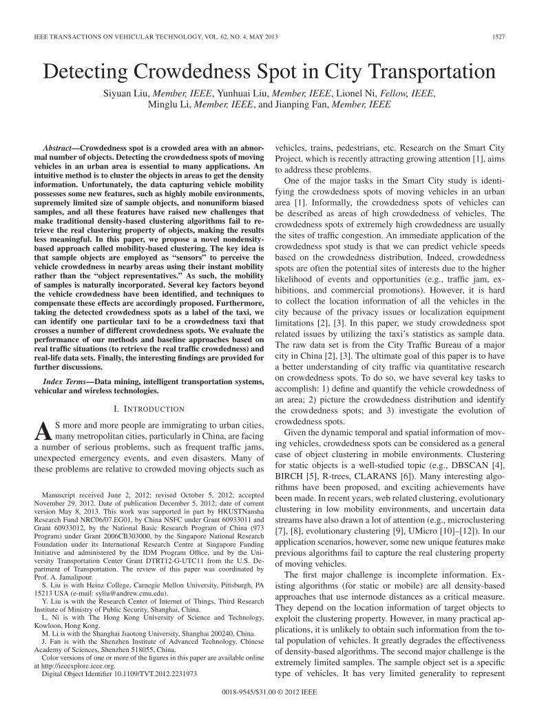
Fig. 12. Flow of the proposed crowdedness taxi intelligent search process.

to create the learning data sets, and utilizes the data sets to trainand build the predictive model. Second, the targeted features arepublished to the users. Third, a user selects a feature of interestto retrieve the relevant list of crowdedness taxis from a searchengine. Fourth, the retrieved taxis are analyzed and classifiedby the predictive model. Finally, only the taxis that are scoredas relevant are sent back to the user.

Definition 8: A taxi trace is a sequence of location samplesfrom the GPS reports in the time order.

Definition 9: Crowdedness taxi is a taxi whose trace crossesa number of different crowdedness spots (the threshold is λ) ina given time interval (t).

If a taxi m crosses a crowdedness spot ls(t)i , we assign 1 tothe taxi at this spot, while if not cross, 0 is assigned. Thus, wecan construct a “0–1” vector for each taxi to record its trace,e.g., xt

m = {0, 1, 1, . . . , 1}.To build the crowdedness taxi classifier, we employ SVM

[13]. Given a set of training vectors xi ∈ Rn, i = 1, 2, . . . , d,where d is the number of vectors, in two cases, and a targetvector y ∈ Rd such that yi ∈ {0, 1}, both classifiers solve thefollowing unconstrained optimization function:

minw

12wTw + C

d∑i=1

�(w;xi, yi) (15)

where C is a positive penalty parameter, and �(w;xi, yi) is aloss function.

In this paper, we choose L2-SVM to build our predictivemodel because of the great efficiency [14]. The evaluation ofthe method is provided in Section VI-C.

VI. FIELD STUDY EVALUATION

In this section, first, we evaluate the crowdedness functionby the real-life data sets (taxi data and bus data), and second,to verify the effectiveness of our mobility-based clustering, wecompare it with the current method on a number of field studies(field camera records) and empirical data sets. Finally, weevaluate the intelligent SVM-based crowdedness taxi classifier.

Fig. 13. Workflow of crowdedness function verification.

A. Crowdedness Function Validation

Our task of validation is to evaluate which of the linear andstatistical crowdedness functions produces a better-fit crowd-edness distribution. We carry out the validation through twoapproaches. One is by conducting the prediction about vehi-cle speed. By this, we look for an optimal configuration formobility-based clustering. The second validation is to comparethe optimal setting mobility-based clustering with traditionalalgorithms through field studies.

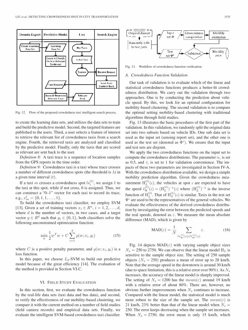
Fig. 13 illustrates the basic procedures of the first part of thevalidation. In this validation, we randomly split the original dataset into two subsets based on vehicle IDs. One sub data set isused as the input set (sensing report set), and the other one isused as the test set (denoted as Φc). We ensure that the inputand test sets are disjoint.

We apply the two crowdedness functions on the input set tocompute the crowdedness distributions. The parameter αι is setas 0.5, and τι is set to 1 for validation convenience. The im-pacts of these two parameters are investigated in Section IV-A.With the crowdedness distribution available, we design a simplemobility prediction algorithm. Given the crowdedness mea-surement H(t)

L (ι), the vehicles at spot ι are expected to have

the speed v(t)Φ (ι) = (H

(t)L )−1(ι) where (H

(t)L )−1 is the inverse

function of H(t)L . That of H(t)

S (ι) is similar. Taxis in the test setΦc are used to be the representatives of the general vehicles. Weevaluate the effectiveness of the derived crowdedness distribu-tion by investigating the error between the predicted speeds andthe real speeds, denoted as ε. We measure the mean absolutedifference (MAD), which is given by

MAD(ε) =1N

∑∀v(t)

Φc (ι)∈V (t)

Φc (ι)

ε. (16)

Fig. 14 depicts MAD(ε) with varying sample object sizesNs = 250 to 2750. We can observe that the linear model HL issensitive to the sample object size. The setting of 250 sampleobjects (Ns = 250) produces a mean of error up to 28 km/h.Note that the average speed in the downtown is around 30 km/h(due to space limitation, this is a relative error over 90%). As Ns

increases, the accuracy of the linear model is sharply improved.The setting of Ns = 1200 has the mean(ε) around 19 km/hwith a relative error of about 80%. There are, however, noobvious further improvements when Ns continues to increase.Compared with the linear model, the statistical model is muchmore robust to the size of the sample set. The mean(ε) is21 km/h, 23% better than that of the linear model when Ns =250. The error keeps decreasing when the sample set increases.When Ns = 2750, the error mean is only 15 km/h, which


Fig. 14. MAD(ε) of linear and statistical models; Ns is from 250 to 2750.

is 50% as the relative error. From the results, we can con-clude that our method achieves better accuracy when the datascale up.

To test the robustness, we validate the crowdedness functionsusing not only the traces of taxis but also traces of 3108 publicbuses.

It is notable that the bus traces are limited to fixed routes.Buses are a specific type of vehicle with more particular movingpatterns. They have regular service routes, periodic movingschedules, and fixed stops. Hence, they are not good enoughto help detect crowdedness spots. However, they are capableof validating our method. We apply the statistical crowdednessfunction on both taxi and bus traces, deriving two crowdednessdistributions. Results show that these two distributions are fairlyconsistent. The consistency is measured by the correlation coef-ficient as defined in Section IV-D. A higher correlation indicatesmore consistency, and the upper limit of the correlation isone that happens only when the two time series are linearlydependent. Note that the average correlation coefficient is up to63%. Over 70% spots have the correlation coefficient ρ between0.6 and 0.8, and about 10% are more than 0.8. Moreover, about20% spots have very low ρ in between. It is mainly becausemost of these spots are bus stops and traffic reconnection sites.In these areas, bus speeds are mainly determined by the sitetype and thus provide little information for spot crowdedness.

In Section IV, we study spot crowdedness in practice. Asa consequence, we find two approaches to reduce the error ofspeed predicting. The first one is to characterize spots, and thesecond one is to profile sensor objects. In Fig. 15, we reportthe evaluation of the first approach, and then we evaluate theimpact from the characteristics of sensor objects. Fig. 15 plotsthe MAD of HS with the simple parameter setting, that is,αι = 0.5, τι = 1, and with the advanced settings of dominatingaverage weight and dominating period. We observe that withthe improved setting, the error can be further reduced by 11%when Ns = 600 and by 15% when Ns = 2400. We concludethat the improved setting is more advantaged under low sampleset scenarios, whereas the advantages are largely revoked bythe larger sample set. With the state calibration by profilingthe sensor objects, the prediction error is further reduced byabout 16% when Ns > 1200. Hence, we can conclude that ourmethod achieves better accuracy when the data scale up.

Fig. 15. Comparison of MAD with simple and optimal parameter settings.

Fig. 16. Number of vehicles produced by three different approaches.

B. Mobility-Based Clustering Validation

To verify the effectiveness of our mobility-based clustering,we conduct a number of field studies. We setup video camerasat predetermined sites in Shanghai, record the real traffic sit-uations in fields, and then measure the crowdedness of theseareas through an offline manner. The results are denoted as“real situation”. Note that in the real situation, we take thecrowdedness as the density of vehicle in the area. On selectingthe comparison method, we choose UMicro, one of the latestrepresentative methods for clustering uncertain data streams[12]. For UMicro, we assume that each taxi in the sampleset represents 80 000 general vehicles, because our data sethas records of 5631 taxis, accounting 0.3% of the two millionof the total vehicle population in the city. For mobility-basedclustering, the produced crowdedness is a relative value. Itneeds an appropriate scalar to generate the absolute vehicledensities. To obtain this scalar, we need to collect the real initialstate of the spot for calibration. In practice, this calibrationusually incurs relatively high cost. We argue, nevertheless, thatthis calibration is a single-run operation such that the high costcan be amortized over a long operation time.

Fig. 16 depicts the real vehicle crowdedness, the estimatednumber by mobility-based clustering, and that by UMicro at thespot of Jiangsu Road over two hours (11:00 A.M. to 13:00 P.M.)on January 15, 2009. Recall the definition of correlation co-efficient defined in Section IV-D. It can be used to measure


TABLE IIMOBILITY-BASED CLUSTERING VERSUS UMICRO

TABLE IIIEVALUATION RESULTS FOR THE PREDICTIVE CLASSIFICATION MODEL

the accuracy of the derived spot crowdedness. Moreover, weutilize precision, recall, and F-score to give insight into theaccuracy. Precision means the percentage of true crowdednessspots in the detected crowdedness spots. Recall means the per-centage of detected true crowdedness spots in true crowdednessspots. F-score is the weighted harmonic mean of precision andrecall [15].

Table II lists the comparison between mobility-based clus-tering and UMicro approach (Appr.). We evaluate the resultsby correlation coefficient (Corr.), precision (Pre.), recall (Rec.),and F-score. The data are from three locations (Loc.). Theresults in the table are the mean results of different thresholds(we test the methods in top-10, top-20, top-30, top-40, and top-50 crowdedness spots’ detection). It shows that at Jiangsu Roadthe results of mobility-based clustering are 10 to 20 times betterthan UMicro under the same scenario. The interesting thinghere is that UMicro performs pretty well at Rail Station. Webelieve this is because the Rail Station is a taxi aggregated areawith high customer flows. Therefore, the samples at this spotare much larger than those at other spots, resulting in a muchbetter accuracy by density-based approaches.

C. Crowdedness Spot Acquisition Validation

We employ one month data to evaluate our SVM-basedintelligent classifying and searching the taxis. A domain ex-pert, such as a transportation officer, can accurately and easilyclassify each taxi’s traces to either relevant or irrelevant tothe taxi of interest (crowdedness taxi in this paper) through aquick inspection of its feature representation. Seven hundredtwenty-eight taxis (12.9% of the total 5631 collected taxis)were classified as relevant to the crowdedness taxis. In theexperiment, recall measures the ability of the model to retrieve agood rate of relevant taxis from the total original relevant taxisavailable, precision measures the rate of really relevant taxisfrom the total taxis that the model has claimed to be relevant,and F-score represents the overall look to both precision andrecall. In Table III, we report the experiment results. The resultsshow that the precision is over 89%, and the recall is over 81%.

VII. FINDINGS AND DISCUSSIONS

In our crowdedness model, we introduce two parameters todescribe the dynamics of the spot in a given location [αι and τιin (4)]. The parameter setting of the dominating average weight

Fig. 17. Categorizing spots by dominating average weight and period.

and the dominating period is unique for each spot and thus canbe utilized to characterize spots. A higher αι indicates lowerdynamism of the spot and larger τι indicates longer period ofspot crowdedness. We therefore categorize spots by presenteddynamism and periods.

Fig. 17 depicts αι and τι of different spots in the weight andperiod plane. We find that the spots are highly aggregated withclustering features. They can be roughly grouped to five groupsnamed from Group I to Group V. Mapping these groups withgeographic information, we have following findings:

1) Group I presents high dynamism and frequent change ofcrowdedness. About 30% spots, a major portion of thespots, belong to this group. Among these spots, over 93%are traffic reconnection sites (e.g., rail station and busconnections).

2) Group II also presents high dynamism but the crowd-edness changing frequency is much lower than that ofGroup I. About 10% spots fall into this category. Over94% of them are shopping and entertainment areas.

3) Group III is mostly traveler’s interests, with 7% spots.4) Group IV accounts another major portion of the spots

with over 40% spots. These spots have steady states andchange gently, which are mostly freeways and express-ways.

5) Group V presents very low dynamism and middle fre-quency of changing. About 8% spots fall into this group,which are mostly working, business, and living areas.

In addition to these five types, there are about 2% outlierspots that can hardly be clearly categorized. An interestingfinding is that the spots in one group are not necessary tobe of the same geographic type. For instance, 7% of Group Ispots are not the traffic reconnection spots but present the samecharacteristic as the spots in Group I. For this, we mainly havetwo hypotheses. One is that this is due to the inappropriateplanning of the city development. In other words, these sitesshould be constructed as the traffic reconnection spots to feedthe traffic requirements. Another is due to the limitation of ourmodel, which is unable to fully distinguish the characteristicsof different sites. By current data we can hardly state whichhypothesis is closer to the reality, while both of them are raisedfor the planning of future city development.


VIII. RELATED WORK

Clustering: Object clustering is a well-studied problem witha great deal of research efforts being devoted in. One of themost promising approaches for spatial static clustering can befound in the research work of DBSCAN [4], [16]. Recently,clustering moving objects has become a crowdedness researchissue. In the research work [7], Li et al. discussed the clusteringof moving objects and extended the concept of microclus-ter. High-quality moving microclusters are dynamically main-tained, which leads to fast and competitive clustering results.Chakrabarti et al. [9] proposed evolutionary clustering, whichis able to well deal with the mobile clusters in low dynamicenvironments. Chen et al. [16] proposed a framework D-Streamto efficiently identify outliers of clusters. Extensive efforts arealso devoted to the clustering with uncertain data [17]–[19],data streams [20], uncertain data streams [8], [12], [18], com-plex event processing [18], [20], co-clustering on large datasets [18], ranking queries [11], [18], [21], and evolutionaryclustering [9], [18]. The above existing works are density-based approaches. In particular, in their study scenario, they allconsider that the density or quantity of the objects is enoughto cluster. Thus, when the density or quantity of the objects isnot that good enough for special application scenarios, they willfail. In our application scenario, these methods do not work dueto the new arising features, such as extreme less samples andnotable data point location errors.

Traffic Data Analysis: Gaffney and Smyth [22] studied theproblem of clustering trajectories and proposed to use short datasequences as object movements. Li et al. [23] studied trafficflow patterns in road networks and proposed a density-basedalgorithm called FlowScan. Kriegel et al. [24] introduced a sta-tistical approach to describe the likelihood of any given individ-ual in road networks to be located at a certain position and time.These works mainly focused on how to accurately measureand predict vehicle speeds while showing very limited insightinto mobile vehicle clustering. Other proposals suggested touse dedicated sensors deployed on roads to perceive vehiclecrowdedness. Benjamin [25] studied how to detect freewayincidents by traffic detectors on roads. Some utilize vehiclesequipped with GPS and/or a cellular positioning system asprobes. Sirvio and Hollmén [26] studied spatiotemporal roadcondition forecasting by Markov chains and artificial neuralnetworks. Castro et al. [27] proposed a method to construct amodel of traffic density based on taxi traces. Bacon et al. [28]tried to use real-time road traffic data to evaluate congestion.Yuan et al. [29] presented a Cloud-based system computingcustomized and practically fast driving routes for an end userusing (historical and real-time) traffic conditions and driverbehavior. Zheng et al. [30] detected flawed urban planningusing the GPS trajectories of taxicabs traveling in urban areas.Liu et al. [31] proposed algorithms to construct outlier causalitytrees based on the temporal and spatial properties of detectedoutliers. Yoon et al. [32] tried to detect traffic conditions onsurface streets given location traces collected from on-road ve-hicles, such as GPS location data and infrequent low-bandwidthcellular updates. The current work assumed that dedicatedsensor devices had been deployed so that the collection of

vehicle crowdedness becomes straightforward. In this paper,we do not have dedicated sensors but employ mobile objects as“sensors” to perceive the crowdedness. The difference betweenour approach and the floating car [33] in intelligent transporta-tion system (ITS) is that the floating car in ITS focuses onthe speed of vehicles, and for crowdedness spot issues, theyhave the common assumptions that each float car representsa number of real vehicles. In our problem, however, taxis arenot good representatives of other vehicles, and therefore, suchapproaches will fail.

IX. CONCLUSION AND FUTURE WORK

In this paper, we have proposed mobility-based clustering,a novel approach to identify crowdedness spots in a highlymobile environment with extremely limited and biased objectsamples. The unique feature of mobility-based clustering isto use speed information to infer the crowdedness of movingobjects. Furthermore, we study the crowdedness spot categoriesand the crowdedness taxi acquisition from the detected crowd-edness spots. We evaluated the performance of mobility-basedclustering based on real taxi data collected in the city throughfield studies. Future work can be conducted along followingdirections. First, in mobility-based clustering, the speed infor-mation is critical. Due to the small sample data set, we useda simple approach to estimate the mobility of vehicles at thespot of no data. Better mobility estimation can produce bettercrowdedness values. Second, there are many factors besidesspot crowdedness that will have impact on vehicle mobility,such as traffic lights and car accidents. We leave them forfuture work. Third, we need more field studies, although laborintensive, to further verify the effectiveness of the mobility-based approach. Fourth, better road griding method is neededfor retrieving much more precious locations. Finally, dependingon other characteristics of moving objects, other nondensity-based clustering may be worth further investigations.

REFERENCES

[1] S. Liu, Y. Liu, L. Ni, J. Fan, and M. Li, “Towards mobility-based cluster-ing,” in Proc. ACM SIGKDD, 2010, pp. 919–928.

[2] H. Zhu, Y. Zhu, M. Li, and L. Ni, “SEER: Metropolitan-scale trafficperception based on lossy sensory data,” in Proc. IEEE INFOCOM, 2009,pp. 217–225.

[3] Smart City Research Group. [Online]. Available: http://www.cse.ust.hk/scrg

[4] J. Sander, M. Ester, H.-P. Kriegel, and X. Xu, “Density-based clustering inspatial databases: The algorithm gdbscan and its applications,” Data Min.Knowl. Discov., vol. 2, no. 2, pp. 169–194, Jun. 1998.

[5] T. Zhang, R. Ramakrishnan, and M. Livny, “BIRCH: An efficient dataclustering method for very large databases,” in Proc. ACM SIGMOD Int.Conf. Manag. Data, 1996, vol. 25, pp. 103–114.

[6] R. T. Ng and J. Han, “CLARANS: A method for clustering objects forspatial data mining,” IEEE Trans. Knowl. Data Eng., vol. 14, no. 5,pp. 1003–1016, Sep./Oct. 2002.

[7] Y. Li, J. Han, and J. Yang, “Clustering moving objects,” in Proc. ACMSIGKDD, 2004, pp. 617–622.

[8] H. Yoon and C. Shahabi, “Robust time-referenced segmentation of mov-ing object trajectories,” in Proc. IEEE ICDM, 2008, pp. 1121–1126.

[9] D. Chakrabarti, R. Kumar, and A. Tomkins, “Evolutionary clustering,” inProc. ACM SIGKDD, 2006, pp. 554–560.

[10] G. Aggarwal, T. Feder, K. Kenthapadi, S. Khuller, R. Panigrahy,D. Thomas, and A. Zhu, “Achieving anonymity via clustering,” in Proc.PODS, 2006, pp. 153–162.


[11] C. Jin, K. Yi, L. Chen, J. X. Yu, and X. Lin, “Sliding-window top-k querieson uncertain streams,” Proc. VLDB Endow., vol. 1, no. 1, pp. 301–312,Aug. 2008.

[12] C. Aggarwal and P. Yu, “A framework for clustering uncertain datastreams,” in Proc. ICDE, 2008, pp. 150–159.

[13] B. E. Boser, I. M. Guyon, and V. N. Vapnik, “A training algorithm foroptimal margin classifiers,” in Proc. COLT , 1992, pp. 144–152.

[14] C. Cortes, M. Mohri, and A. Rostamizadeh, “L2 regularization for learn-ing kernels,” in Proc. UAI, 2009, pp. 109–116.

[15] R. A. Baeza-Yates and B. Ribeiro-Neto, Modern Information Retrieval.Reading, MA: Addison-Wesley, 1999.

[16] Y. Chen and L. Tu, “Density-based clustering for real-time stream data,”in Proc. ACM SIGKDD, 2007, pp. 133–142.

[17] B. Kao, S. D. Lee, D. W. Cheung, W.-S. Ho, and K. F. Chan, “Clusteringuncertain data using Voronoi diagrams,” in Proc. IEEE ICDM, 2008,pp. 333–342.

[18] T. Xu, Z. M. Zhang, P. S. Yu, and B. Long, “Evolutionary clustering byhierarchical Dirichlet process with hidden Markov state,” in Proc. IEEEICDM, 2008, pp. 658–667.

[19] F. Gullo, G. Ponti, A. Tagarelli, and S. Greco, “A hierarchical algorithmfor clustering uncertain data via an information-theoretic approach,” inProc. IEEE ICDM, 2008, pp. 821–826.

[20] T. Li and S. S. Anand, “HIREL: An incremental clustering algorithm forrelational datasets,” in Proc. IEEE ICDM, 2008, pp. 887–892.

[21] J. Pei, M. Hua, Y. Tao, and X. Lin, “Query answering techniques on un-certain and probabilistic data: tutorial summary,” in Proc. ACM SIGMOD,2008, pp. 1357–1364.

[22] S. Gaffney and P. Smyth, “Trajectory clustering with mixtures of regres-sion models,” in Proc. ACM SIGKDD, 1999, pp. 63–72.

[23] X. Li, J. Han, J.-G. Lee, and H. Gonzalez, “Traffic density-based discov-ery of hot routes in road networks,” in Proc. SSTD, 2007, pp. 441–459.

[24] H.-P. Kriegel, M. Renz, M. Schubert, and A. Zuefle, “Statistical densityprediction in traffic networks,” in Proc. IEEE ICDM, 2007, pp. 887–892.

[25] C. Benjamin, “Detecting the onset of congestion rapidly with existingtraffic detectors,” Transp. Res. Part A: Policy and Practice, vol. 37, no. 3,2003.

[26] K. Sirvio and J. Hollmén, “Spatio-temporal road condition forecastingwith Markov chains and artificial neural networks,” in Proc. HAIS, 2008,pp. 204–211.

[27] P. S. Castro, D. Zhang, and S. Li, “Urban traffic modelling and predictionusing large scale taxi GPS traces,” in Proc. Pervasive, 2012, pp. 57–72.

[28] J. Bacon, A. I. Bejan, A. R. Beresford, D. Evans, R. J. Gibbens, andK. Moody, “Using real-time road traffic data to evaluate cngestion,” inDependable and Historic Computing, vol. 6875, Lecture Notes in Com-puter Science. Berlin, Germany: Springer-Verlag, 2011, pp. 93–117.

[29] J. Yuan, Y. Zheng, X. Xie, and G. Sun, “Driving with knowledge from thephysical world,” in Proc. ACM SIGKDD, 2011, pp. 316–324.

[30] Y. Zheng, Y. Liu, J. Yuan, and X. Xie, “Urban computing with taxicabs,”in Proc. UbiComp, 2011, pp. 89–98.

[31] W. Liu, Y. Zheng, S. Chawla, J. Yuan, and X. Xing, “Discoveringspatio-temporal causal interactions in traffic data streams,” in Proc. ACMSIGKDD, 2011, pp. 1010–1018.

[32] J. Yoon, B. Noble, and M. Liu, “Surface street traffic estimation,” in Proc.ACM MobiSys, 2007, pp. 220–232.

[33] S. Messelodi, C. M. Modena, M. Zanin, F. G. B. De Natale, F. Granelli,E. Betterle, and A. Guarise, “Intelligent extended floating car data collec-tion,” Expert Syst. Appl., vol. 36, no. 3, pp. 4213–4227, Apr. 2009.

Siyuan Liu (M’12) received the Ph.D. degree fromThe Hong Kong University of Science and Technol-ogy, Kowloon, Hong Kong, in 2011.

He is a Researcher Scientist with Heinz Col-lege, Carnegie Mellon University, Pittsburgh, PA.His research interests include data mining in spatio-temporal data, time series, and social networks.

Yunhuai Liu (M’09) received the Ph.D. degreein computer science and engineering from TheHong Kong University of Science and Technology,Kowloon, Hong Kong, in 2008.

From 2008 to 2010, he was a Research AssistantProfessor with The Hong Kong University of Scienceand Technology. In 2011, he joined the ResearchCenter of Internet of Things, Third Research Instituteof Ministry of Public Security, Shanghai, China. Hisresearch papers have been published in many pres-tigious conferences and journals such as the ACM

Mobicom, IEEE INFOCOM, IEEE ICDCS, IEEE ICPADS, IEEE TPDS, andIEEE TMC. His paper entitled "Opportunity-based topology control in wirelesssensor networks" received the only Best Paper Award at the 2008 IEEE ICDCS(one out of 638). His research interests include wireless sensor networks,cognitive radio networks, and extreme-scale datacenter and data networks.

Lionel Ni (F’94) is a Chair Professor with the De-partment of Computer Science and Engineering, TheHong Kong University of Science and Technology(HKUST), Kowloon, Hong Kong. He also serves asthe Special Assistant to the President of HKUST,as Dean of the HKUST Fok Ying Tung GraduateSchool, and as a Visiting Chair Professor of theShanghai Key Laboratory of Scalable Computingand Systems, Shanghai Jiao Tong University, Shang-hai, China.

Dr. Ni has chaired over 30 professional confer-ences and has received six awards for authoring outstanding papers.

Minglu Li (M’00) received the Ph.D. degree in com-puter software from Shanghai Jiao Tong University,Shanghai, China, in 1996.

He is a Full Professor, the Vice Dean of the Schoolof Electronics Information and Electrical Engineer-ing, and the Director of the Grid Computing Center,Shanghai Jiao Tong University. He has publishedmore than 100 papers in academic journals and inter-national conferences. His current research interestsinclude grid computing, services computing, andsensor networks.

Dr. Li is a Member of the Executive Committee of the Technical Committeeon Services Computing of the IEEE Computer Society.

Jianping Fan (M’00) received the Ph.D. degreefrom the Institute of Software, Chinese Academy ofSciences (CAS), Beijing, China, in 1990.

From 1990 to 2006, he was with the Instituteof Computing Technology, where he served as theDeputy Chief Engineer of the National ResearchCenter for Intelligent Computing Systems, the Di-rector of the National Engineering Center on HighPerformance Computing, and the Vice Director ofthe Institute of Computing Technology. Since 2006,he has served as Director of the Shenzhen Institute

of Advanced Technology, CAS. He took part in and developed Dawning I,Dawning 1000, Dawning 3000, Dawning 4000, and other series of Dawningsupercomputers. He has published more than 70 papers and one book. Hisresearch interests include high-performance computing, grid computing, andcomputer architecture.

city crowd

Documents

thevehicle crowdedness

crowdedness taxi thatcrosses

detected crowdedness

moving objects

ieee transactions

abnormal number of objects

mobilitybased clustering

yunhuai liu