cise 302 linear control systems laboratory manual - …€¦ · 2 lab experiment 1: using matlab...
TRANSCRIPT
King Fahd University of Petroleum & Minerals
CISE 302
Linear Control Systems
Laboratory Manual Systems Engineering Department
Revised - September 2012

2 Lab Experiment 1: Using MATLAB for Control Systems
CISE 302 Lab Manual Page 2
Table of Contents
Lab Experiment 1: Using MATLAB for Control Systems ................................................................ 4
Part I: Introduction to MATLAB ........................................................................................................ 4
Part II: Polynomials in MATLAB .................................................................................................... 15
Part III: Scripts, Functions & Flow Control in MATLAB ................................................................ 19
Laboratory Experiment 2: Mathematical Modeling of Physical Systems ..................................... 26
Mass-Spring System Model .......................................................................................................... 26
Speed Cruise Control example: ..................................................................................................... 28
Mass-Spring System Example: ..................................................................................................... 29
Exercise 1 .......................................................................................................................................... 30
Exercise 2 .......................................................................................................................................... 30
Laboratory Experiment 3: Modeling of Physical Systems using SIMULINK .............................. 31
Overview: ...................................................................................................................................... 31
Mass-Spring System Model .......................................................................................................... 36
Exercise 1: Modeling of a second order system ................................................................................ 37
Exercise 2: Simulation with system parameter variation .................................................................. 39
Exercise 3: System response from the stored energy with zero input ............................................... 40
Exercise 4: Cruise System ................................................................................................................ 40
Laboratory Experiment 4: Linear Time-invariant Systems and Representation ......................... 41
Objectives: This experiment has following two objectives: ............................................................. 41
Mass-Spring System Model .......................................................................................................... 41
Transfer Function: ......................................................................................................................... 42
Linear Time-Invariant Systems in MATLAB: .............................................................................. 42
Examples of Creating LTI Models ................................................................................................ 42
Simulation of Linear systems to different inputs .............................................................................. 44
Exercise 1: ......................................................................................................................................... 46
Exercise 2: ......................................................................................................................................... 46
Exercise 3: ......................................................................................................................................... 46
Exercise 4: ......................................................................................................................................... 46
Lab Experiment 5: Block Diagram Reduction ................................................................................. 47
Exercise 1: ......................................................................................................................................... 51
Exercise 2: ......................................................................................................................................... 51
Exercise 3: ......................................................................................................................................... 52
Lab Experiment 6: Performance of First order and second order systems .................................. 53
3 Lab Experiment 1: Using MATLAB for Control Systems
CISE 302 Lab Manual Page 3
Exercise 1: ......................................................................................................................................... 54
Exercise 2: ......................................................................................................................................... 56
Lab Experiment 7: DC Motor Characteristics ................................................................................. 57
Model of the armature-controlled DC motor: ................................................................................... 58
Model Simulation using Simulink: ................................................................................................... 59
Parameter Identification: ................................................................................................................... 65
Lab Experiment 8: Validation of DC Motor Characteristics ......................................................... 68
Model validation: .............................................................................................................................. 68
Nonlinear characteristics ................................................................................................................... 70
Lab Experiment 9: Effect of Feedback on disturbance & Control System Design ....................... 74
Lab Experiment 10: Effect of Feedback on disturbance & Control System Design of Tank Level
System .................................................................................................................................................. 78
Lab Experiment 11: Introduction to PID controller ....................................................................... 80
Lab Experiment 12: Open Loop and Closed Loop position control of DC Motor ........................ 88
Lab Experiment 13: Simple Speed Control of DC Motor ............................................................... 94
Lab Experiment 14: PID Controller Design for Two Tank System ............................................. 101
Part – I: Design of Proportional Control in the PID Controller ...................................................... 103
Part – II: Design of Integral Part in the PID Controller .................................................................. 107

4 Lab Experiment 1: Using MATLAB for Control Systems
CISE 302 Lab Manual Page 4
CISE 302
Linear Control Systems
Lab Experiment 1: Using MATLAB for Control Systems
Objectives: This lab provides an introduction to MATLAB in the first part. The lab also
provides tutorial of polynomials, script writing and programming aspect of MATLAB from
control systems view point.
List of Equipment/Software
Following equipment/software is required:
MATLAB
Category Soft-Experiment
Deliverables
A complete lab report including the following:
Summarized learning outcomes.
MATLAB scripts and their results should be reported properly.
Part I: Introduction to MATLAB
Objective: The objective of this exercise will be to introduce you to the concept of
mathematical programming using the software called MATLAB. We shall study how to
define variables, matrices etc, see how we can plot results and write simple MATLAB codes.
MATLAB TUTORIAL
Reference: Engineering Problem Solving Using MATLAB, by Professor Gary Ford, University of California, Davis.
___________________________________
___________________________________
___________________________________
___________________________________
___________________________________
___________________________________
___________________________________
5 Lab Experiment 1: Using MATLAB for Control Systems
CISE 302 Lab Manual Page 5
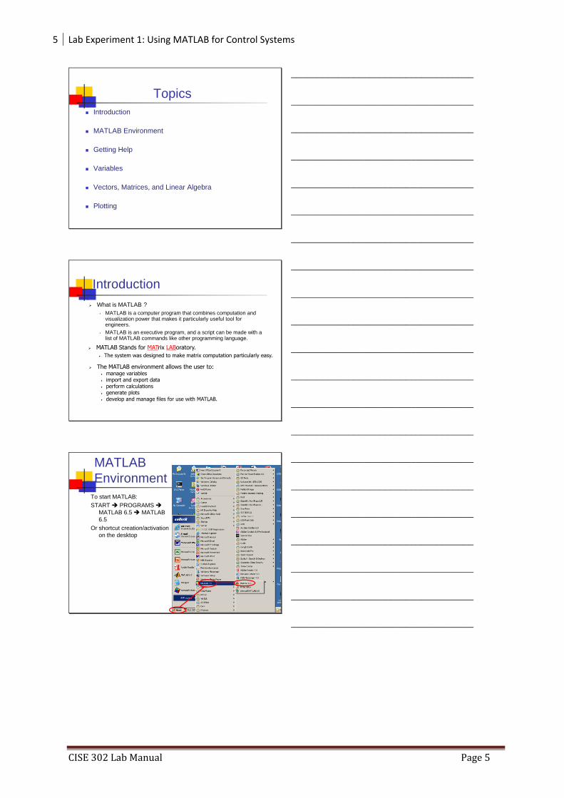
Topics
Introduction
MATLAB Environment
Getting Help
Variables
Vectors, Matrices, and Linear Algebra
Plotting
___________________________________
___________________________________
___________________________________
___________________________________
___________________________________
___________________________________
___________________________________
Introduction
What is MATLAB ?
• MATLAB is a computer program that combines computation and visualization power that makes it particularly useful tool for engineers.
• MATLAB is an executive program, and a script can be made with a list of MATLAB commands like other programming language.
MATLAB Stands for MATrix LABoratory.
• The system was designed to make matrix computation particularly easy.
The MATLAB environment allows the user to:• manage variables• import and export data• perform calculations• generate plots• develop and manage files for use with MATLAB.
___________________________________
___________________________________
___________________________________
___________________________________
___________________________________
___________________________________
___________________________________
MATLAB
Environment
To start MATLAB:
START PROGRAMS
MATLAB 6.5 MATLAB
6.5
Or shortcut creation/activation
on the desktop
___________________________________
___________________________________
___________________________________
___________________________________
___________________________________
___________________________________
___________________________________

6 Lab Experiment 1: Using MATLAB for Control Systems
CISE 302 Lab Manual Page 6
Display Windows
___________________________________
___________________________________
___________________________________
___________________________________
___________________________________
___________________________________
___________________________________
Display Windows (con’t…)
Graphic (Figure) Window
Displays plots and graphs
Created in response to graphics
commands.
M-file editor/debugger window
Create and edit scripts of commands called
M-files.
___________________________________
___________________________________
___________________________________
___________________________________
___________________________________
___________________________________
___________________________________
Getting Help
type one of following commands in the command window: help – lists all the help topic
help topic – provides help for the specified topic
help command – provides help for the specified command
help help – provides information on use of the help command
helpwin – opens a separate help window for navigation
lookfor keyword – Search all M-files for keyword
___________________________________
___________________________________
___________________________________
___________________________________
___________________________________
___________________________________
___________________________________

7 Lab Experiment 1: Using MATLAB for Control Systems
CISE 302 Lab Manual Page 7
Variables
Variable names:
Must start with a letter
May contain only letters, digits, and the underscore “_”
Matlab is case sensitive, i.e. one & OnE are different variables.
Matlab only recognizes the first 31 characters in a variable name.
Assignment statement:
Variable = number;
Variable = expression;
Example:
>> tutorial = 1234;
>> tutorial = 1234
tutorial =
1234
NOTE: when a semi-colon ”;” is placed at the end of each command, the result is not displayed.
___________________________________
___________________________________
___________________________________
___________________________________
___________________________________
___________________________________
___________________________________
Variables (con’t…)
Special variables: ans : default variable name for the result
pi: = 3.1415926…………
eps: = 2.2204e-016, smallest amount by which 2 numbers can differ.
Inf or inf : , infinity
NaN or nan: not-a-number
Commands involving variables: who: lists the names of defined variables
whos: lists the names and sizes of defined variables
clear: clears all varialbes, reset the default values of special variables.
clear name: clears the variable name
clc: clears the command window
clf: clears the current figure and the graph window.
___________________________________
___________________________________
___________________________________
___________________________________
___________________________________
___________________________________
___________________________________
Vectors, Matrices and Linear Algebra
Vectors
Matrices
Array Operations
Solutions to Systems of Linear
Equations.
___________________________________
___________________________________
___________________________________
___________________________________
___________________________________
___________________________________
___________________________________
8 Lab Experiment 1: Using MATLAB for Control Systems
CISE 302 Lab Manual Page 8
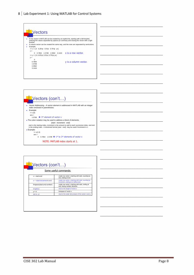
Vectors
A row vector in MATLAB can be created by an explicit list, starting with a left bracket, entering the values separated by spaces (or commas) and closing the vector with a right bracket.
A column vector can be created the same way, and the rows are separated by semicolons.
Example:
>> x = [ 0 0.25*pi 0.5*pi 0.75*pi pi ]
x =
0 0.7854 1.5708 2.3562 3.1416
>> y = [ 0; 0.25*pi; 0.5*pi; 0.75*pi; pi ]
y =
0
0.7854
1.5708
2.3562
3.1416
x is a row vector.
y is a column vector.
___________________________________
___________________________________
___________________________________
___________________________________
___________________________________
___________________________________
___________________________________
Vectors (con’t…)
Vector Addressing – A vector element is addressed in MATLAB with an integer
index enclosed in parentheses.
Example:
>> x(3)
ans =
1.5708
1st to 3rd elements of vector x
The colon notation may be used to address a block of elements.
(start : increment : end)
start is the starting index, increment is the amount to add to each successive index, and end
is the ending index. A shortened format (start : end) may be used if increment is 1.
Example:
>> x(1:3)
ans =
0 0.7854 1.5708
NOTE: MATLAB index starts at 1.
3rd element of vector x
___________________________________
___________________________________
___________________________________
___________________________________
___________________________________
___________________________________
___________________________________
Vectors (con’t…)Some useful commands:
x = start:end create row vector x starting with start, counting by one, ending at end
x = start:increment:end create row vector x starting with start, counting by increment, ending at or before end
linspace(start,end,number) create row vector x starting with start, ending at end, having number elements
length(x) returns the length of vector x
y = x’ transpose of vector x
dot (x, y) returns the scalar dot product of the vector x and y.
___________________________________
___________________________________
___________________________________
___________________________________
___________________________________
___________________________________
___________________________________

9 Lab Experiment 1: Using MATLAB for Control Systems
CISE 302 Lab Manual Page 9
Matrices
A is an m x n matrix.
A Matrix array is two-dimensional, having both multiple rows and multiple columns,
similar to vector arrays:
it begins with [, and end with ]
spaces or commas are used to separate elements in a row
semicolon or enter is used to separate rows.
•Example:
>> f = [ 1 2 3; 4 5 6]
f =
1 2 3
4 5 6
>> h = [ 2 4 6
1 3 5]
h =
2 4 6
1 3 5the main diagonal
___________________________________
___________________________________
___________________________________
___________________________________
___________________________________
___________________________________
___________________________________
Matrices (con’t…)
Magic Function
For example you can generate a matrix by entering
>> m=magic(4)
It generates a matrix whose elements are such that the sum of all elements in its rows, columns and diagonal elements are same
Sum Function
You can verify the above magic square by entering
>> sum(m)
For rows take the transpose and then take the sum
>> sum(m’)
Diag
You can get the diagonal elements of a matrix by entering
>> d=diag(m)
>> sum(d)
___________________________________
___________________________________
___________________________________
___________________________________
___________________________________
___________________________________
___________________________________
Matrices (con’t…)
Matrix Addressing:
-- matrixname(row, column)
-- colon may be used in place of a row or column reference to select the entire row or column.
recall:f =
1 2 34 5 6
h =2 4 61 3 5
Example:
>> f(2,3)
ans =
6
>> h(:,1)
ans =
2
1
___________________________________
___________________________________
___________________________________
___________________________________
___________________________________
___________________________________
___________________________________
10 Lab Experiment 1: Using MATLAB for Control Systems
CISE 302 Lab Manual Page 10
Matrices (con’t…)
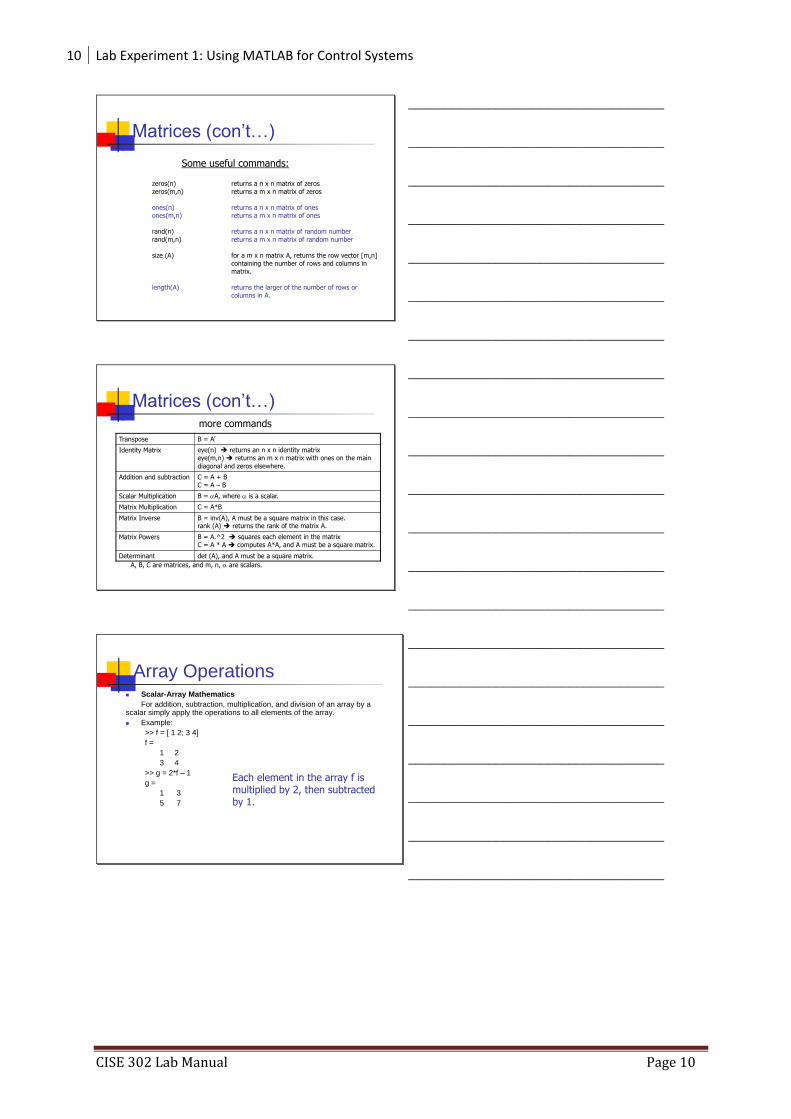
Some useful commands:
zeros(n)zeros(m,n)
ones(n)ones(m,n)
rand(n)rand(m,n)
size (A)
length(A)
returns a n x n matrix of zerosreturns a m x n matrix of zeros
returns a n x n matrix of onesreturns a m x n matrix of ones
returns a n x n matrix of random numberreturns a m x n matrix of random number
for a m x n matrix A, returns the row vector [m,n] containing the number of rows and columns in matrix.
returns the larger of the number of rows or columns in A.
___________________________________
___________________________________
___________________________________
___________________________________
___________________________________
___________________________________
___________________________________
Matrices (con’t…)
Transpose B = A’
Identity Matrix eye(n) returns an n x n identity matrixeye(m,n) returns an m x n matrix with ones on the main
diagonal and zeros elsewhere.
Addition and subtraction C = A + BC = A – B
Scalar Multiplication B = A, where is a scalar.
Matrix Multiplication C = A*B
Matrix Inverse B = inv(A), A must be a square matrix in this case.rank (A) returns the rank of the matrix A.
Matrix Powers B = A.^2 squares each element in the matrixC = A * A computes A*A, and A must be a square matrix.
Determinant det (A), and A must be a square matrix.
more commands
A, B, C are matrices, and m, n, are scalars.
___________________________________
___________________________________
___________________________________
___________________________________
___________________________________
___________________________________
___________________________________
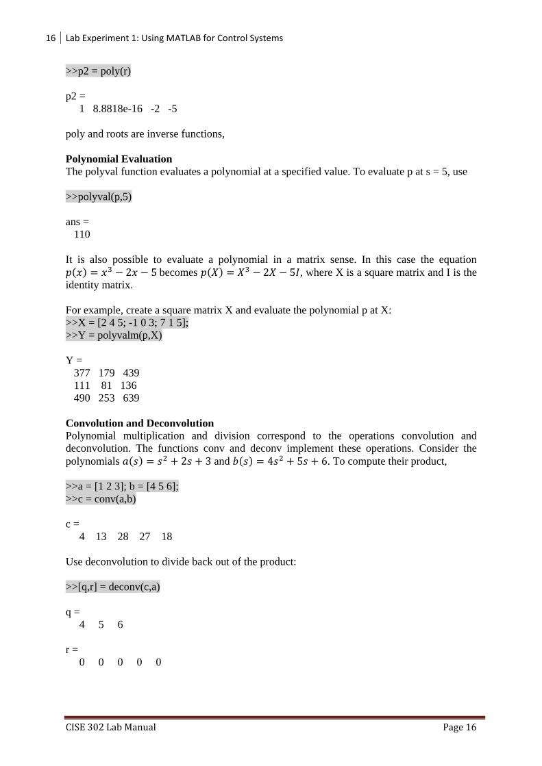
Array Operations Scalar-Array Mathematics
For addition, subtraction, multiplication, and division of an array by a scalar simply apply the operations to all elements of the array.
Example:
>> f = [ 1 2; 3 4]
f =
1 2
3 4
>> g = 2*f – 1
g =
1 3
5 7
Each element in the array f is multiplied by 2, then subtracted by 1.
___________________________________
___________________________________
___________________________________
___________________________________
___________________________________
___________________________________
___________________________________

11 Lab Experiment 1: Using MATLAB for Control Systems
CISE 302 Lab Manual Page 11
Array Operations (con’t…)
Element-by-Element Array-Array Mathematics.
Operation Algebraic Form MATLAB
Addition a + b a + b
Subtraction a – b a – b
Multiplication a x b a .* b
Division a b a ./ b
Exponentiation ab a .^ b
Example:>> x = [ 1 2 3 ];
>> y = [ 4 5 6 ];
>> z = x .* y
z =
4 10 18
Each element in x is multiplied by the corresponding element in y.
___________________________________
___________________________________
___________________________________
___________________________________
___________________________________
___________________________________
___________________________________
Solutions to Systems of Linear Equations
Example: a system of 3 linear equations with 3 unknowns (x1, x2, x3):
3x1 + 2x2 – x3 = 10
-x1 + 3x2 + 2x3 = 5
x1 – x2 – x3 = -1
Then, the system can be described as:
Ax = b
111
231
123
A
3
2
1
x
x
x
x
1
5
10
b
Let :
___________________________________
___________________________________
___________________________________
___________________________________
___________________________________
___________________________________
___________________________________
Solutions to Systems of Linear Equations
(con’t…)
Solution by Matrix Inverse:Ax = b
A-1Ax = A-1b
x = A-1b
MATLAB:>> A = [ 3 2 -1; -1 3 2; 1 -1 -1];
>> b = [ 10; 5; -1];
>> x = inv(A)*b
x =
-2.0000
5.0000
-6.0000
Answer:
x1 = -2, x2 = 5, x3 = -6
Solution by Matrix Division:The solution to the equation
Ax = bcan be computed using left division.
Answer:
x1 = -2, x2 = 5, x3 = -6
NOTE: left division: A\b b A right division: x/y x y
MATLAB:>> A = [ 3 2 -1; -1 3 2; 1 -1 -1];
>> b = [ 10; 5; -1];
>> x = A\b
x =
-2.0000
5.0000
-6.0000
___________________________________
___________________________________
___________________________________
___________________________________
___________________________________
___________________________________
___________________________________

12 Lab Experiment 1: Using MATLAB for Control Systems
CISE 302 Lab Manual Page 12
Plotting For more information on 2-D plotting, type help graph2d
Plotting a point:
>> plot ( variablename, ‘symbol’)the function plot () creates a graphics window, called a Figure window, and named by default “Figure No. 1”
Example : Complex number>> z = 1 + 0.5j;>> plot (z, ‘.’)
commands for axes:
command description
axis ([xmin xmax ymin ymax]) Define minimum and maximum values of the axes
axis square Produce a square plot
axis equal equal scaling factors for both axes
axis normal turn off axis square, equal
axis (auto) return the axis to defaults
___________________________________
___________________________________
___________________________________
___________________________________
___________________________________
___________________________________
___________________________________
Plotting (con’t…) Plotting Curves:
plot (x,y) – generates a linear plot of the values of x (horizontal axis) and y (vertical axis).
semilogx (x,y) – generate a plot of the values of x and y using a logarithmic scale for x and a linear scale for y
semilogy (x,y) – generate a plot of the values of x and y using a linear scale for x and a logarithmic scale for y.
loglog(x,y) – generate a plot of the values of x and y using logarithmic scales for both x and y
___________________________________
___________________________________
___________________________________
___________________________________
___________________________________
___________________________________
___________________________________
Plotting (con’t…) Multiple Curves:
plot (x, y, w, z) – multiple curves can be plotted on the same graph by using multiple arguments in a plot command. The variables x, y, w, and z are vectors. Two curves will be plotted: y vs. x, and z vs. w.
legend (‘string1’, ‘string2’,…) – used to distinguish between plots on the same graph
Multiple Figures: figure (n) – used in creation of multiple plot windows. place this command
before the plot() command, and the corresponding figure will be labeled as “Figure n”
close – closes the figure n window.
close all – closes all the figure windows.
Subplots: subplot (m, n, p) – m by n grid of windows, with p specifying the
current plot as the pth window
___________________________________
___________________________________
___________________________________
___________________________________
___________________________________
___________________________________
___________________________________

13 Lab Experiment 1: Using MATLAB for Control Systems
CISE 302 Lab Manual Page 13
Plotting (con’t…) Example: (polynomial function)
plot the polynomial using linear/linear scale, log/linear scale, linear/log scale, & log/log scale:
y = 2x2 + 7x + 9
% Generate the polynomial:
x = linspace (0, 10, 100);
y = 2*x.^2 + 7*x + 9;
% plotting the polynomial:
figure (1);
subplot (2,2,1), plot (x,y);
title ('Polynomial, linear/linear scale');
ylabel ('y'), grid;
subplot (2,2,2), semilogx (x,y);
title ('Polynomial, log/linear scale');
ylabel ('y'), grid;
subplot (2,2,3), semilogy (x,y);
title ('Polynomial, linear/log scale');
xlabel('x'), ylabel ('y'), grid;
subplot (2,2,4), loglog (x,y);
title ('Polynomial, log/log scale');
xlabel('x'), ylabel ('y'), grid;
___________________________________
___________________________________
___________________________________
___________________________________
___________________________________
___________________________________
___________________________________
Plotting (con’t…)
___________________________________
___________________________________
___________________________________
___________________________________
___________________________________
___________________________________
___________________________________
Plotting (con’t…) Adding new curves to the existing graph:
Use the hold command to add lines/points to an existing plot.
hold on – retain existing axes, add new curves to current axes. Axes are rescaled when necessary.
hold off – release the current figure window for new plots
Grids and Labels:
Command Description
grid on Adds dashed grids lines at the tick marks
grid off removes grid lines (default)
grid toggles grid status (off to on, or on to off)
title (‘text’) labels top of plot with text in quotes
xlabel (‘text’) labels horizontal (x) axis with text is quotes
ylabel (‘text’) labels vertical (y) axis with text is quotes
text (x,y,’text’) Adds text in quotes to location (x,y) on the current axes, where (x,y) is in units from the current plot.
___________________________________
___________________________________
___________________________________
___________________________________
___________________________________
___________________________________
___________________________________
14 Lab Experiment 1: Using MATLAB for Control Systems
CISE 302 Lab Manual Page 14
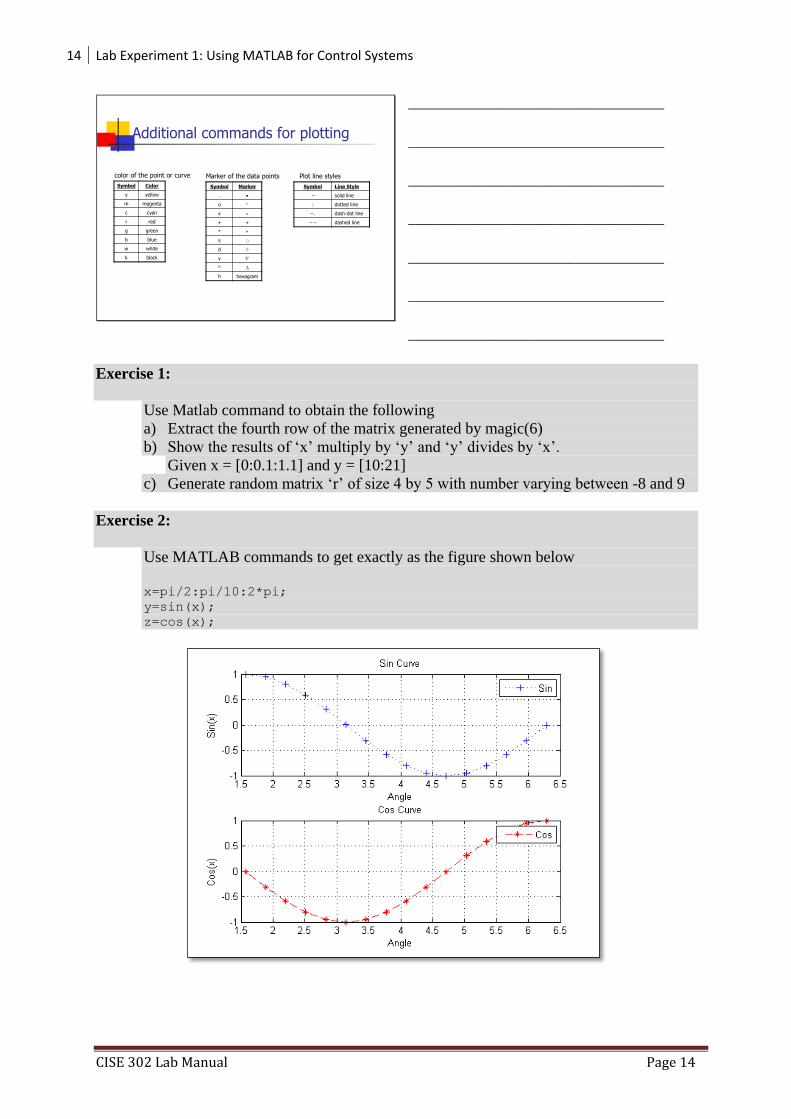
Additional commands for plotting
Symbol Color
y yellow
m magenta
c cyan
r red
g green
b blue
w white
k black
Symbol Marker
.
o
x
+ +
*
s
d ◊
v
^
h hexagram
color of the point or curve Marker of the data points Plot line styles
Symbol Line Style
– solid line
: dotted line
–. dash-dot line
– – dashed line
___________________________________
___________________________________
___________________________________
___________________________________
___________________________________
___________________________________
___________________________________
Exercise 1:
Use Matlab command to obtain the following
a) Extract the fourth row of the matrix generated by magic(6)
b) Show the results of ‘x’ multiply by ‘y’ and ‘y’ divides by ‘x’.
Given x = [0:0.1:1.1] and y = [10:21]
c) Generate random matrix ‘r’ of size 4 by 5 with number varying between -8 and 9
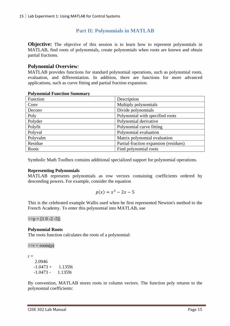
Exercise 2:
Use MATLAB commands to get exactly as the figure shown below
x=pi/2:pi/10:2*pi; y=sin(x); z=cos(x);
15 Lab Experiment 1: Using MATLAB for Control Systems
CISE 302 Lab Manual Page 15
Part II: Polynomials in MATLAB
Objective: The objective of this session is to learn how to represent polynomials in
MATLAB, find roots of polynomials, create polynomials when roots are known and obtain
partial fractions.
Polynomial Overview: MATLAB provides functions for standard polynomial operations, such as polynomial roots,
evaluation, and differentiation. In addition, there are functions for more advanced
applications, such as curve fitting and partial fraction expansion.
Polynomial Function Summary
Function Description
Conv Multiply polynomials
Deconv Divide polynomials
Poly Polynomial with specified roots
Polyder Polynomial derivative
Polyfit Polynomial curve fitting
Polyval Polynomial evaluation
Polyvalm Matrix polynomial evaluation
Residue Partial-fraction expansion (residues)
Roots Find polynomial roots
Symbolic Math Toolbox contains additional specialized support for polynomial operations.
Representing Polynomials
MATLAB represents polynomials as row vectors containing coefficients ordered by
descending powers. For example, consider the equation
( )
This is the celebrated example Wallis used when he first represented Newton's method to the
French Academy. To enter this polynomial into MATLAB, use
>>p = [1 0 -2 -5];
Polynomial Roots
The roots function calculates the roots of a polynomial:
>>r = roots(p)
r =
2.0946
-1.0473 + 1.1359i
-1.0473 - 1.1359i
By convention, MATLAB stores roots in column vectors. The function poly returns to the
polynomial coefficients:
16 Lab Experiment 1: Using MATLAB for Control Systems
CISE 302 Lab Manual Page 16
>>p2 = poly(r)
p2 =
1 8.8818e-16 -2 -5
poly and roots are inverse functions,
Polynomial Evaluation
The polyval function evaluates a polynomial at a specified value. To evaluate p at s = 5, use
>>polyval(p,5)
ans =
110
It is also possible to evaluate a polynomial in a matrix sense. In this case the equation
( ) becomes ( ) , where X is a square matrix and I is the
identity matrix.
For example, create a square matrix X and evaluate the polynomial p at X:
>>X = [2 4 5; -1 0 3; 7 1 5];
>>Y = polyvalm(p,X)
Y =
377 179 439
111 81 136
490 253 639
Convolution and Deconvolution
Polynomial multiplication and division correspond to the operations convolution and
deconvolution. The functions conv and deconv implement these operations. Consider the
polynomials ( ) and ( ) . To compute their product,
>>a = [1 2 3]; b = [4 5 6];
>>c = conv(a,b)
c =
4 13 28 27 18
Use deconvolution to divide back out of the product:
>>[q,r] = deconv(c,a)
q =
4 5 6
r =
0 0 0 0 0
17 Lab Experiment 1: Using MATLAB for Control Systems
CISE 302 Lab Manual Page 17
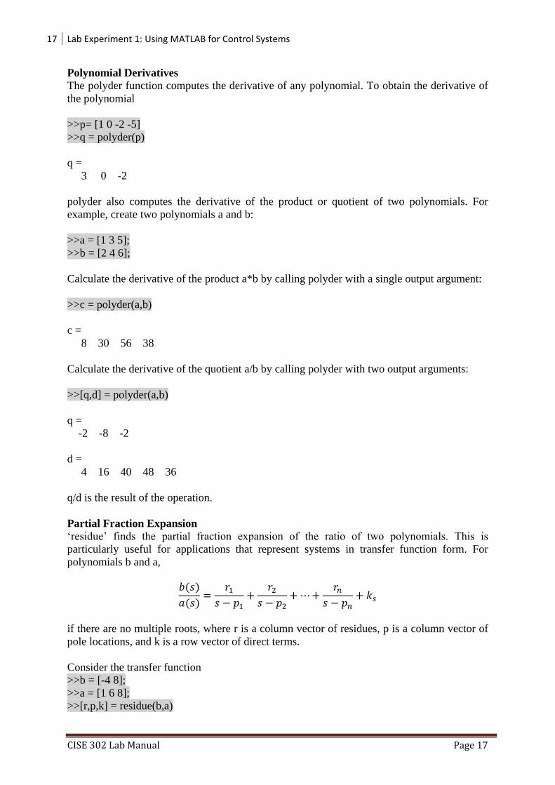
Polynomial Derivatives
The polyder function computes the derivative of any polynomial. To obtain the derivative of
the polynomial
>>p= [1 0 -2 -5]
>>q = polyder(p)
q =
3 0 -2
polyder also computes the derivative of the product or quotient of two polynomials. For
example, create two polynomials a and b:
>>a = [1 3 5];
>>b = [2 4 6];
Calculate the derivative of the product a*b by calling polyder with a single output argument:
>>c = polyder(a,b)
c =
8 30 56 38
Calculate the derivative of the quotient a/b by calling polyder with two output arguments:
>>[q,d] = polyder(a,b)
q =
-2 -8 -2
d =
4 16 40 48 36
q/d is the result of the operation.
Partial Fraction Expansion
‘residue’ finds the partial fraction expansion of the ratio of two polynomials. This is
particularly useful for applications that represent systems in transfer function form. For
polynomials b and a,
( )
( )
if there are no multiple roots, where r is a column vector of residues, p is a column vector of
pole locations, and k is a row vector of direct terms.
Consider the transfer function
>>b = [-4 8];
>>a = [1 6 8];
>>[r,p,k] = residue(b,a)

18 Lab Experiment 1: Using MATLAB for Control Systems
CISE 302 Lab Manual Page 18
r =
-12
8
p =
-4
-2
k =
[]
Given three input arguments (r, p, and k), residue converts back to polynomial form:
>>[b2,a2] = residue(r,p,k)
b2 =
-4 8
a2 =
1 6 8
Exercise 1:
Consider the two polynomials ( ) and ( ) . Using
MATLAB compute
a. ( ) ( ) b. Roots of ( ) and ( ) c. ( ) and ( )
Exercise 2:
Use MATLAB command to find the partial fraction of the following
a. ( )
( )
b. ( )
( )
( )
19 Lab Experiment 1: Using MATLAB for Control Systems
CISE 302 Lab Manual Page 19
Part III: Scripts, Functions & Flow Control in MATLAB
Objective: The objective of this session is to introduce you to writing M-file scripts,
creating MATLAB Functions and reviewing MATLAB flow control like ‘if-elseif-end’, ‘for
loops’ and ‘while loops’.
Overview: MATLAB is a powerful programming language as well as an interactive computational
environment. Files that contain code in the MATLAB language are called M-files. You create
M-files using a text editor, then use them as you would any other MATLAB function or
command. There are two kinds of M-files:
Scripts, which do not accept input arguments or return output arguments. They
operate on data in the workspace. MATLAB provides a full programming language
that enables you to write a series of MATLAB statements into a file and then execute
them with a single command. You write your program in an ordinary text file, giving
the file a name of ‘filename.m’. The term you use for ‘filename’ becomes the new
command that MATLAB associates with the program. The file extension of .m makes
this a MATLAB M-file.
Functions, which can accept input arguments and return output arguments. Internal
variables are local to the function.
If you're a new MATLAB programmer, just create the M-files that you want to try out in the
current directory. As you develop more of your own M-files, you will want to organize them
into other directories and personal toolboxes that you can add to your MATLAB search path.
If you duplicate function names, MATLAB executes the one that occurs first in the search
path.
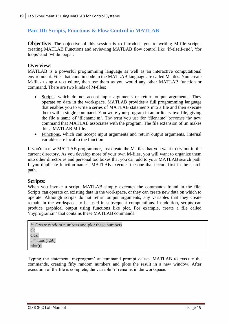
Scripts: When you invoke a script, MATLAB simply executes the commands found in the file.
Scripts can operate on existing data in the workspace, or they can create new data on which to
operate. Although scripts do not return output arguments, any variables that they create
remain in the workspace, to be used in subsequent computations. In addition, scripts can
produce graphical output using functions like plot. For example, create a file called
‘myprogram.m’ that contains these MATLAB commands:
Typing the statement ‘myprogram’ at command prompt causes MATLAB to execute the
commands, creating fifty random numbers and plots the result in a new window. After
execution of the file is complete, the variable ‘r’ remains in the workspace.
% Create random numbers and plot these numbers clc clear r = rand(1,50) plot(r)

20 Lab Experiment 1: Using MATLAB for Control Systems
CISE 302 Lab Manual Page 20
Functions: Functions are M-files that can accept input arguments and return output arguments. The
names of the M-file and of the function should be the same. Functions operate on variables
within their own workspace, separate from the workspace you access at the MATLAB
command prompt. An example is provided below:
M-File Element Description
Function definition line
(functions only)
Defines the function name, and the number and order of input and
output arguments.
H1 line A one line summary description of the program, displayed when
you request help on an entire directory, or when you use
‘lookfor’.
Help text A more detailed description of the program, displayed together
with the H1 line when you request help on a specific function
Function or script body Program code that performs the actual computations and assigns
values to any output arguments.
Comments Text in the body of the program that explains the internal
workings of the program.
The first line of a function M-file starts with the keyword ‘function’. It gives the function
name and order of arguments. In this case, there is one input arguments and one output
argument. The next several lines, up to the first blank or executable line, are comment lines
that provide the help text. These lines are printed when you type ‘help fact’. The first line of
the help text is the H1 line, which MATLAB displays when you use the ‘lookfor’ command
or request help on a directory. The rest of the file is the executable MATLAB code defining
the function.
The variable n & f introduced in the body of the function as well as the variables on the first
line are all local to the function; they are separate from any variables in the MATLAB
workspace. This example illustrates one aspect of MATLAB functions that is not ordinarily
found in other programming languages—a variable number of arguments. Many M-files
work this way. If no output argument is supplied, the result is stored in ans. If the second
input argument is not supplied, the function computes a default value.
Flow Control:
Conditional Control – if, else, switch
This section covers those MATLAB functions that provide conditional program control. if,
else, and elseif. The if statement evaluates a logical expression and executes a group of
statements when the expression is true. The optional elseif and else keywords provide for the
function f = fact(n) Function definition line % Compute a factorial value. H1 line % FACT(N) returns the factorial of N, Help text % usually denoted by N!
% Put simply, FACT(N) is PROD(1:N). Comment f = prod(1:n); Function body
21 Lab Experiment 1: Using MATLAB for Control Systems
CISE 302 Lab Manual Page 21
execution of alternate groups of statements. An end keyword, which matches the if,
terminates the last group of statements.
The groups of statements are delineated by the four keywords—no braces or brackets are
involved as given below.
if <condition>
<statements>;
elseif <condition>
<statements>;
else
<statements>;
end
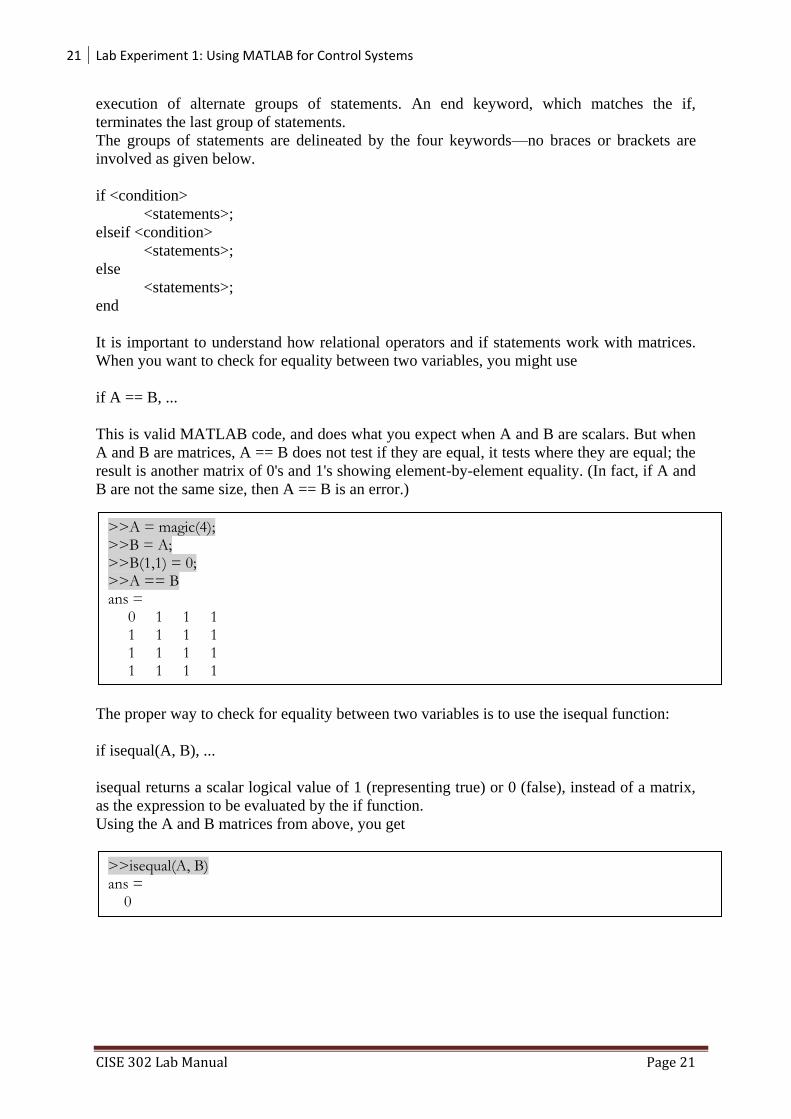
It is important to understand how relational operators and if statements work with matrices.
When you want to check for equality between two variables, you might use
if A == B, ...
This is valid MATLAB code, and does what you expect when A and B are scalars. But when
A and B are matrices, A == B does not test if they are equal, it tests where they are equal; the
result is another matrix of 0's and 1's showing element-by-element equality. (In fact, if A and
B are not the same size, then A == B is an error.)
The proper way to check for equality between two variables is to use the isequal function:
if isequal(A, B), ...
isequal returns a scalar logical value of 1 (representing true) or 0 (false), instead of a matrix,
as the expression to be evaluated by the if function.
Using the A and B matrices from above, you get
>>A = magic(4); >>B = A; >>B(1,1) = 0; >>A == B ans = 0 1 1 1 1 1 1 1 1 1 1 1 1 1 1 1
>>isequal(A, B) ans = 0
22 Lab Experiment 1: Using MATLAB for Control Systems
CISE 302 Lab Manual Page 22
Here is another example to emphasize this point. If A and B are scalars, the following
program will never reach the "unexpected situation". But for most pairs of matrices, including
our magic squares with interchanged columns, none of the matrix conditions A > B, A < B,
or A == B is true for all elements and so the else clause is executed:
Several functions are helpful for reducing the results of matrix comparisons to scalar
conditions for use with if, including ‘isequal’, ‘isempty’, ‘all’, ‘any’.
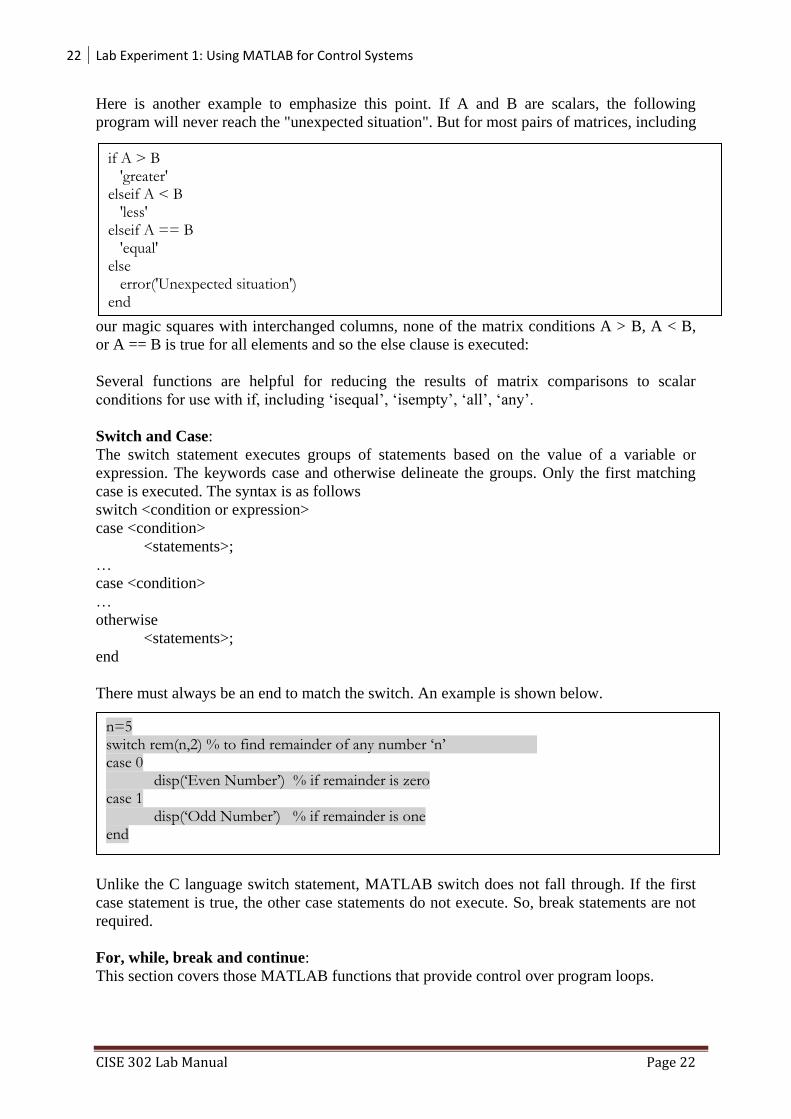
Switch and Case:
The switch statement executes groups of statements based on the value of a variable or
expression. The keywords case and otherwise delineate the groups. Only the first matching
case is executed. The syntax is as follows
switch <condition or expression>
case <condition>
<statements>;
…
case <condition>
…
otherwise
<statements>;
end
There must always be an end to match the switch. An example is shown below.
Unlike the C language switch statement, MATLAB switch does not fall through. If the first
case statement is true, the other case statements do not execute. So, break statements are not
required.
For, while, break and continue:
This section covers those MATLAB functions that provide control over program loops.
if A > B 'greater' elseif A < B 'less' elseif A == B 'equal' else error('Unexpected situation') end
n=5 switch rem(n,2) % to find remainder of any number ‘n’ case 0 disp(‘Even Number’) % if remainder is zero case 1 disp(‘Odd Number’) % if remainder is one end
23 Lab Experiment 1: Using MATLAB for Control Systems
CISE 302 Lab Manual Page 23
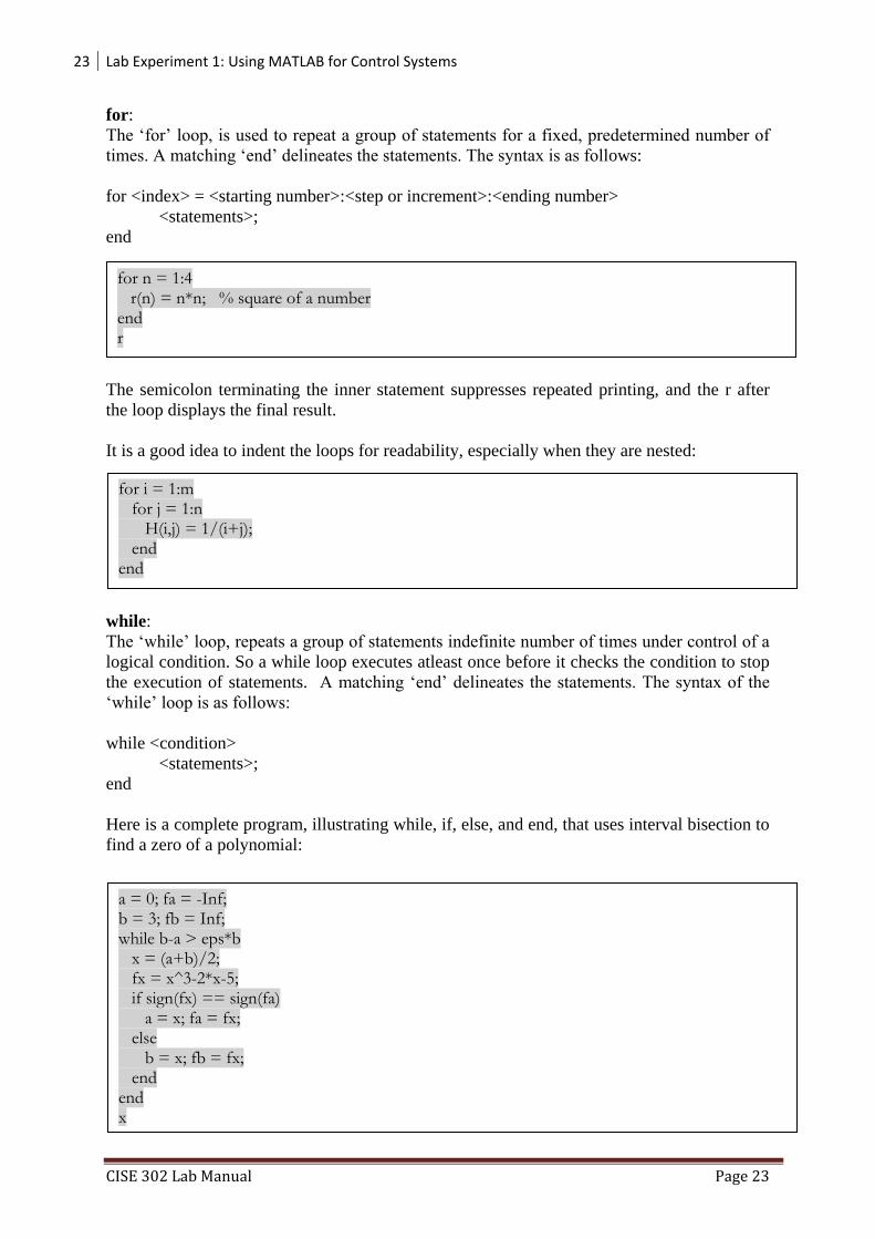
for:
The ‘for’ loop, is used to repeat a group of statements for a fixed, predetermined number of
times. A matching ‘end’ delineates the statements. The syntax is as follows:
for <index> = <starting number>:<step or increment>:<ending number>
<statements>;
end
The semicolon terminating the inner statement suppresses repeated printing, and the r after
the loop displays the final result.
It is a good idea to indent the loops for readability, especially when they are nested:
while:
The ‘while’ loop, repeats a group of statements indefinite number of times under control of a
logical condition. So a while loop executes atleast once before it checks the condition to stop
the execution of statements. A matching ‘end’ delineates the statements. The syntax of the
‘while’ loop is as follows:
while <condition>
<statements>;
end
Here is a complete program, illustrating while, if, else, and end, that uses interval bisection to
find a zero of a polynomial:
for n = 1:4 r(n) = n*n; % square of a number end r
for i = 1:m for j = 1:n H(i,j) = 1/(i+j); end end
a = 0; fa = -Inf; b = 3; fb = Inf; while b-a > eps*b x = (a+b)/2; fx = x^3-2*x-5; if sign(fx) == sign(fa) a = x; fa = fx; else b = x; fb = fx; end end x
24 Lab Experiment 1: Using MATLAB for Control Systems
CISE 302 Lab Manual Page 24
The result is a root of the polynomial x3 - 2x - 5, namely x = 2.0945. The cautions involving
matrix comparisons that are discussed in the section on the if statement also apply to the
while statement.
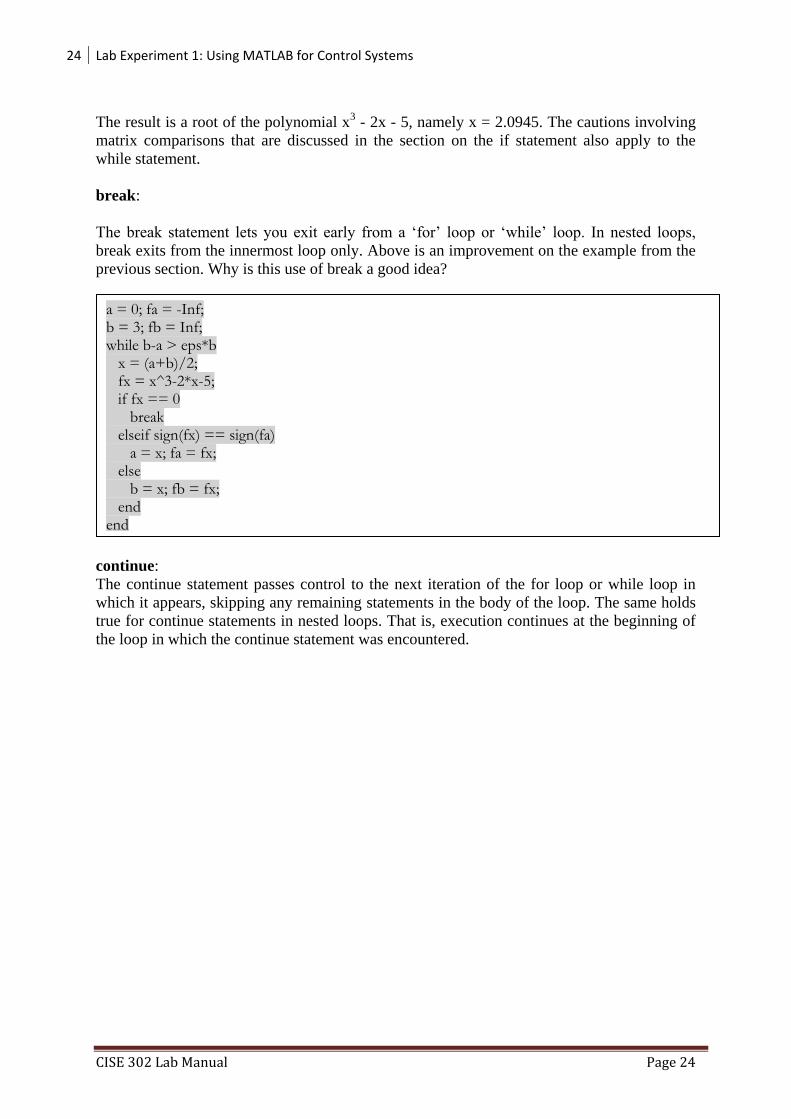
break:
The break statement lets you exit early from a ‘for’ loop or ‘while’ loop. In nested loops,
break exits from the innermost loop only. Above is an improvement on the example from the
previous section. Why is this use of break a good idea?
continue:
The continue statement passes control to the next iteration of the for loop or while loop in
which it appears, skipping any remaining statements in the body of the loop. The same holds
true for continue statements in nested loops. That is, execution continues at the beginning of
the loop in which the continue statement was encountered.
a = 0; fa = -Inf; b = 3; fb = Inf; while b-a > eps*b x = (a+b)/2; fx = x^3-2*x-5; if fx == 0 break elseif sign(fx) == sign(fa) a = x; fa = fx; else b = x; fb = fx; end end
25 Lab Experiment 1: Using MATLAB for Control Systems
CISE 302 Lab Manual Page 25
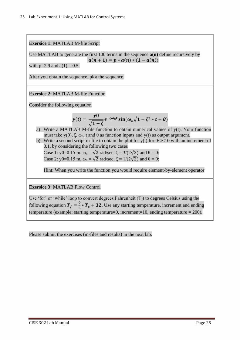
Exersice 1: MATLAB M-file Script
Use MATLAB to generate the first 100 terms in the sequence a(n) define recursively by
( ) ( ) ( ( )) with p=2.9 and a(1) = 0.5.
After you obtain the sequence, plot the sequence.
Exersice 2: MATLAB M-file Function
Consider the following equation
( )
√ ( √
)
a) Write a MATLAB M-file function to obtain numerical values of y(t). Your function
must take y(0), ζ, ωn, t and θ as function inputs and y(t) as output argument.
b) Write a second script m-file to obtain the plot for y(t) for 0<t<10 with an increment of
0.1, by considering the following two cases
Case 1: y0=0.15 m, ωn = √ rad/sec, ζ = 3/(2√ ) and θ = 0;
Case 2: y0=0.15 m, ωn = √ rad/sec, ζ = 1/(2√ ) and θ = 0;
Hint: When you write the function you would require element-by-element operator
Exersice 3: MATLAB Flow Control
Use ‘for’ or ‘while’ loop to convert degrees Fahrenheit (Tf) to degrees Celsius using the
following equation
. Use any starting temperature, increment and ending
temperature (example: starting temperature=0, increment=10, ending temperature = 200).
Please submit the exercises (m-files and results) in the next lab.
26 Laboratory Experiment 2: Mathematical Modeling of Physical Systems
CISE 302 Lab Manual Page 26
CISE 302
Linear Control Systems
Laboratory Experiment 2: Mathematical Modeling of Physical Systems
Objectives: The objective of this exercise is to grasp the important role mathematical
models of physical systems in the design and analysis of control systems. We will learn how
MATLAB helps in solving such models.
List of Equipment/Software
Following equipment/software is required:
MATLAB
Category Soft-Experiment
Deliverables
A complete lab report including the following:
Summarized learning outcomes.
MATLAB scripts and their results for all the assignments and exercises should be
properly reported.
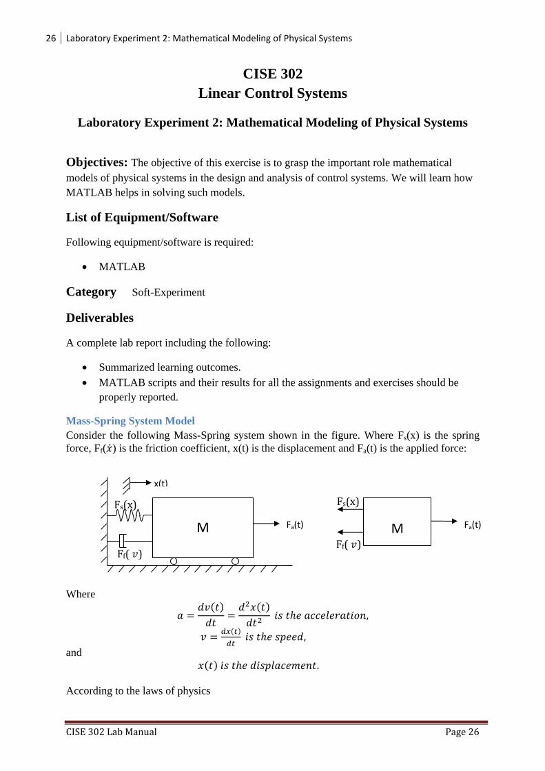
Mass-Spring System Model
Consider the following Mass-Spring system shown in the figure. Where Fs(x) is the spring
force, Ff( ) is the friction coefficient, x(t) is the displacement and Fa(t) is the applied force:
Where
( )
( )
( )
and
( )
According to the laws of physics
Fs(x)
M
Ff( 𝑣)
Fa(t)
x(t)
M Fa(t)
Ff( 𝑣)
Fs(x)

27 Laboratory Experiment 2: Mathematical Modeling of Physical Systems
CISE 302 Lab Manual Page 27
( ) ( ) ( ) (1)
In the case where:
( ) ( )
( ) ( )
The differential equation for the above Mass-Spring system can then be written as follows
( )
( )
( ) ( ) (2)
B is called the friction coefficient and K is called the spring constant.
The linear differential equation of second order (2) describes the relationship between the
displacement and the applied force. The differential equation can then be used to study the
time behavior of x(t) under various changes of the applied force. In reality, the spring force
and/or the friction force can have a more complicated expression or could be represented by a
graph or data table. For instance, a nonlinear spring can be designed (see figure 4.2) such that
( ) ( ) Where r > 1.
Figure 4.2: MAG nonlinear spring (www.tokyo-model.com.hk/ecshop/goods.php?id=2241)
In such case, (1) becomes
( )
( )
( ) ( ) (3)
Equation (3) represents another possible model that describes the dynamic behavior of the
mass-damper system under external force. Model (2) is said to be a linear model whereas (3)
is said to be nonlinear. To decide if a system is linear or nonlinear two properties have to be
verified homogeneity and superposition.
Assignment: use homogeneity and superposition properties to show that model (1) is linear
whereas model (3) is nonlinear.
Solving the differential equation using MATLAB:
The objectives behind modeling the mass-damper system can be many and may include
Understanding the dynamics of such system
28 Laboratory Experiment 2: Mathematical Modeling of Physical Systems
CISE 302 Lab Manual Page 28
Studying the effect of each parameter on the system such as mass M, the friction
coefficient B, and the elastic characteristic Fs(x).
Designing a new component such as damper or spring.
Reproducing a problem in order to suggest a solution.
The solution of the difference equations (1), (2), or (3) leads to finding x(t) subject to certain
initial conditions.
MATLAB can help solve linear or nonlinear ordinary differential equations (ODE). To show
how you can solve ODE using MATLAB we will proceed in two steps. We first see how can
we solve first order ODE and second how can we solve equation (2) or (3).
Speed Cruise Control example:
Assume the spring force ( ) which means that K=0. Equation (2) becomes
( )
( )
( ) (4)
Or
( )
( ) (5)
Equation (5) is a first order linear ODE.
Using MATLAB solver ode45 we can write do the following:
1_ create a MATLAB-function cruise_speed.m
function dvdt=cruise_speed(t, v)
%flow rate
M=750; %(Kg)
B=30; %( Nsec/m)
Fa=300; %N
% dv/dt=Fa/M-B/M v
dvdt=Fa/M-B/M*v;
2_ create a new MATLAB m-file and write
v0= 0; %(initial speed)
[t,v]=ode45('cruise_speed', [0 125],v0);
plot(t,v); grid on;
title('cruise speed time response to a constant traction force Fa(t) ')
29 Laboratory Experiment 2: Mathematical Modeling of Physical Systems
CISE 302 Lab Manual Page 29
There are many other MATLAB ODE solvers such as ode23, ode45, ode113, ode15s, etc…
The function dsolve will result in a symbolic solution. Do ‘doc dsolve’ to know more. In
MATLAB write
>>dsolve(‘Dv=Fa/M-B/M*v’, ‘v(0)=0’)
Note that using MATLAB ODE solvers are able to solve linear or nonlinear ODE’s. We will
see in part II of this experiment another approach to solve a linear ODE differently. Higher
order systems can also be solved similarly.
Mass-Spring System Example:
Assume the spring force ( ) ( ). The mass-spring damper is now equivalent to
( )
( )
( ) ( )
The second order differential equation has to be decomposed in a set of first order differential
equations as follows
Variables New
variable
Differential equation
x(t) X1
dx(t)/dt X2
( )
( )
In vector form, let [ ] ;
[
] then the system can be written as
[
( )
( )
]
The ode45 solver can be now be used:
1_ create a MATLAB-function mass_spring.m
Function dXdt=mass_spring(t, X)
%flow rate
M=750; %(Kg)
B=30; %( Nsec/m)
Fa=300; %N
K=15; %(N/m)
r=1;
% dX/dt
30 Laboratory Experiment 2: Mathematical Modeling of Physical Systems
CISE 302 Lab Manual Page 30
Mass dis-
placement y(t) Mass
M
Spring
Constant k Forcing
Function f(t)
k
Friction
Constant b
dXdt(1,1)=X(2);
dXdt(2,1)=-B/M*X(2)-K/M*X(1)^r+Fa/M;
2_ in MATLAB write
>> X0=[0; 0]; %(initial speed and position)
>> options = odeset('RelTol',[1e-4 1e-4],'AbsTol',[1e-5 1e-5],'Stats','on');
>>[t,X]=ode45('mass_spring', [0 200],X0);
Exercise 1
1. Plot the position and the speed in separate graphs.
2. Change the value of r to 2 and 3.
3. Superpose the results and compare with the linear case r=1 and plot all three cases in the
same plot window. Please use different figures for velocity and displacement.
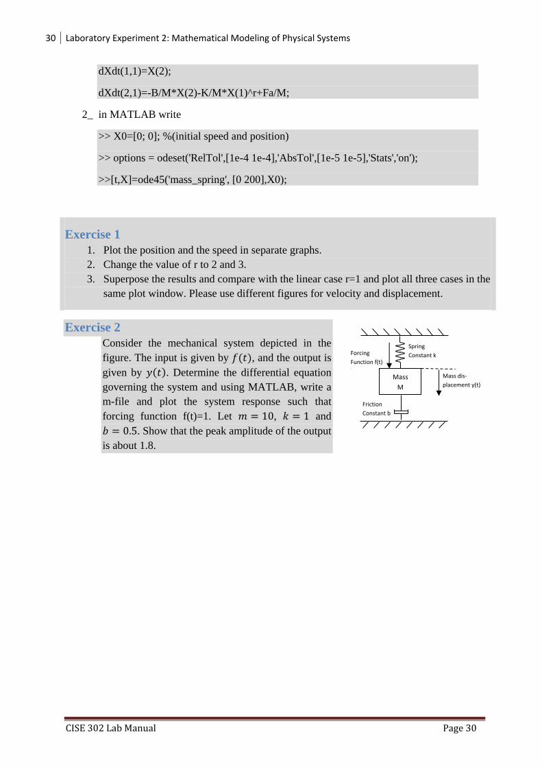
Exercise 2
Consider the mechanical system depicted in the
figure. The input is given by ( ), and the output is
given by ( ). Determine the differential equation
governing the system and using MATLAB, write a
m-file and plot the system response such that
forcing function f(t)=1. Let , and
. Show that the peak amplitude of the output
is about 1.8.

31 Laboratory Experiment 3: Modeling of Physical Systems using SIMULINK
CISE 302 Lab Manual Page 31
CISE 302
Linear Control Systems
Laboratory Experiment 3: Modeling of Physical Systems using SIMULINK
Objectives: The objective of this exercise is to use graphical user interface diagrams to
model the physical systems for the purpose of design and analysis of control systems. We
will learn how MATLAB/SIMULINK helps in solving such models.
List of Equipment/Software
Following equipment/software is required:
MATLAB/SIMULINK
Category Soft-Experiment
Deliverables
A complete lab report including the following:
Summarized learning outcomes.
MATLAB scripts, SIMULINK diagrams and their results for all the assignments and
exercises should be properly reported.
Overview:
This lab introduces powerful graphical user interface (GUI), Simulink of Matlab. This
software is used for solving the modeling equations and obtaining the response of a system to
different inputs. Both linear and nonlinear differential equations can be solved numerically
with high precision and speed, allowing system responses to be calculated and displayed for
many input functions. To provide an interface between a system’s modeling equations and
the digital computer, block diagrams drawn from the system’s differential equations are used.
A block diagram is an interconnection of blocks representing basic mathematical operations
in such a way that the overall diagram is equivalent to the system’s mathematical model. The
lines interconnecting the blocks represent the variables describing the system behavior. These
may be inputs, outputs, state variables, or other related variables. The blocks represent
operations or functions that use one or more of these variables to calculate other variables.
Block diagrams can represent modeling equations in both input-output and state variable
form.
We use MATLAB with its companion package Simulink, which provides a graphical user
interface (GUI) for building system models and executing the simulation. These models are
constructed by drawing block diagrams representing the algebraic and differential equations
that describe the system behavior. The operations that we generally use in block diagrams are
summation, gain, and integration. Other blocks, including nonlinear elements such as

32 Laboratory Experiment 3: Modeling of Physical Systems using SIMULINK
CISE 302 Lab Manual Page 32
multiplication, square root, exponential, logarithmic, and other functions, are available.
Provisions are also included for supplying input functions, using a signal generator block,
constants etc and for displaying results, using a scope block.
An important feature of a numerical simulation is the ease with which parameters can be
varied and the results observed directly. MATLAB is used in a supporting role to initialize
parameter values and to produce plots of the system response. Also MATLAB is used for
multiple runs for varying system parameters. Only a small subset of the functions of
MATLAB will be considered during these labs.
SIMULINK
Simulink provides access to an extensive set of blocks that accomplish a wide range of
functions useful for the simulation and analysis of dynamic systems. The blocks are grouped
into libraries, by general classes of functions.
Mathematical functions such as summers and gains are in the Math library.
Integrators are in the Continuous library.
Constants, common input functions, and clock can all be found in the Sources library.
Scope, To Workspace blocks can be found in the Sinks library.
Simulink is a graphical interface that allows the user to create programs that are actually run
in MATLAB. When these programs run, they create arrays of the variables defined in
Simulink that can be made available to MATLAB for analysis and/or plotting. The variables
to be used in MATLAB must be identified by Simulink using a “To Workspace” block,
which is found in the Sinks library. (When using this block, open its dialog box and specify
that the save format should be Matrix, rather than the default, which is called Structure.) The
Sinks library also contains a Scope, which allows variables to be displayed as the simulated
system responds to an input. This is most useful when studying responses to repetitive inputs.
Simulink uses blocks to write a program. Blocks are arranged in various libraries according
to their functions. Properties of the blocks and the values can be changed in the associated
dialog boxes. Some of the blocks are given below.
SUM (Math library)
A dialog box obtained by double-clicking on the SUM block performs the configuration of
the SUM block, allowing any number of inputs and the sign of each. The sum block can be
represented in two ways in Simulink, by a circle or by a rectangle. Both choices are shown
Figure 1: Two Simulink blocks for a summer representing y = x 1+ x2 – x3
X1
X2
X3
X1
X2
X3

33 Laboratory Experiment 3: Modeling of Physical Systems using SIMULINK
CISE 302 Lab Manual Page 33
GAIN (Math library)
A gain block is shown by a triangular symbol, with the gain expression written inside if it
will fit. If not, the symbol - k - is used. The value used in each gain block is established in a
dialog box that appears if the user double-clicks on its block.
Figure 2: Simulink block for a gain of K.
INTEGRATOR (Continuous library)
The block for an integrator as shown below looks unusual. The quantity 1/s comes from the
Laplace transform expression for integration. When double-clicked on the symbol for an
integrator, a dialog box appears allowing the initial condition for that integrator to be
specified. It may be implicit, and not shown on the block, as in Figure (a). Alternatively, a
second input to the block can be displayed to supply the initial condition explicitly, as in part
(b) of Figure 3. Initial conditions may be specific numerical values, literal variables, or
algebraic expressions.
Figure3: Two forms of the Simulink block for an integrator.
(a) Implicit initial condition. (b) Explicit initial condition.
CONSTANTS (Source library)
Constants are created by the Constant block, which closely resembles Figure 4. Double-
clicking on the symbol opens a dialog box to establish the constant’s value. It can be a
number or an algebraic expression using constants whose values are defined in the workspace
and are therefore known to MATLAB.
Figure 4: A constant block
34 Laboratory Experiment 3: Modeling of Physical Systems using SIMULINK
CISE 302 Lab Manual Page 34
STEP (Source library)
A Simulink block is provided for a Step input, a signal that changes (usually from zero) to a
specified new, constant level at a specified time. These levels and time can be specified
through the dialog box, obtained by double-clicking on the Step block.
Figure 5: A step block
SIGNAL GENERATOR (Source library)
One source of repetitive signals in Simulink is called the Signal Generator. Double-clicking
on the Signal Generator block opens a dialog box, where a sine wave, a square wave, a ramp
(sawtooth), or a random waveform can be chosen. In addition, the amplitude and frequency
of the signal may be specified. The signals produced have a mean value of zero. The
repetition frequency can be given in Hertz (Hz), which is the same as cycles per second, or in
radians/second.
Figure 6: A signal generator block
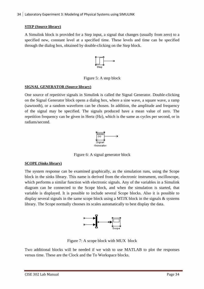
SCOPE (Sinks library)
The system response can be examined graphically, as the simulation runs, using the Scope
block in the sinks library. This name is derived from the electronic instrument, oscilloscope,
which performs a similar function with electronic signals. Any of the variables in a Simulink
diagram can be connected to the Scope block, and when the simulation is started, that
variable is displayed. It is possible to include several Scope blocks. Also it is possible to
display several signals in the same scope block using a MTJX block in the signals & systems
library. The Scope normally chooses its scales automatically to best display the data.
Figure 7: A scope block with MUX block
Two additional blocks will be needed if we wish to use MATLAB to plot the responses
versus time. These are the Clock and the To Workspace blocks.
35 Laboratory Experiment 3: Modeling of Physical Systems using SIMULINK
CISE 302 Lab Manual Page 35
CLOCK (Sources library)
The clock produces the variable “time” that is associated with the integrators as MATLAB
calculates a numerical (digital) solution to a model of a continuous system. The result is a
string of sample values of each of the output variables. These samples are not necessarily at
uniform time increments, so it is necessary to have the variable “time” that contains the time
corresponding to each sample point. Then MATLAB can make plots versus “time.” The
clock output could be given any arbitrary name; we use “t” in most of the cases.
Figure 8: A clock block
To Workspace (Sinks library)
The To Workspace block is used to return the results of a simulation to the MATLAB
workspace, where they can be analyzed and/or plotted. Any variable in a Simulink diagram
can be connected to a ToWorkspace block. In our exercises, all of the state variables and the
input variables are usually returned to the workspace. In addition, the result of any output
equation that may be simulated would usually be sent to the workspace. In the block
parameters drop down window, change the save format to ‘array’.
Figure 9: A To Workspace block
In the Simulink diagram, the appearance of a block can be changed by changing the
foreground or background colours, or by drop shadow or other options available in the format
drop down menu. The available options can be reached in the Simulink window by
highlighting the block, then clicking the right mouse button. The Show Drop Shadow option
is on the format drop-down menu.
Simulink provides scores of other blocks with different functions.
You are encouraged to browse the Simulink libraries and consult the online Help facility
provided with MATLAB.
GENERAL INSTRUCTIONS FOR WRITING A SIMULINK PROGRAM
To create a simulation in Simulink, follow the steps:
Start MATLAB.
Start Simulink.

36 Laboratory Experiment 3: Modeling of Physical Systems using SIMULINK
CISE 302 Lab Manual Page 36
Open the libraries that contain the blocks you will need. These usually will include
the Sources, Sinks, Math and Continuous libraries, and possibly others.
Open a new Simulink window.
Drag the needed blocks from their library folders to that window. The Math library,
for example, contains the Gain and Sum blocks.
Arrange these blocks in an orderly way corresponding to the equations to be solved.
Interconnect the blocks by dragging the cursor from the output of one block to the
input of another block. Interconnecting branches can be made by right-clicking on an
existing branch.
Double-click on any block having parameters that must be established, and set these
parameters. For example, the gain of all Gain blocks must be set. The number and
signs of the inputs to a Sum block must be established. The parameters of any source
blocks should also be set in this way.
It is necessary to specify a stop time for the solution. This is done by clicking on the
Simulation > Parameters entry on the Simulink toolbar.
At the Simulation > Parameters entry, several parameters can be selected in this dialog box,
but the default values of all of them should be adequate for almost all of the exercises. If the
response before time zero is needed, it can be obtained by setting the Start time to a negative
value. It may be necessary in some problems to reduce the maximum integration step size
used by the numerical algorithm. If the plots of the results of a simulation appear “choppy” or
composed of straight-line segments when they should be smooth, reducing the max step size
permitted can solve this problem.
Mass-Spring System Model
Consider the Mass-Spring system used in the previous exercise as shown in the figure. Where
Fs(x) is the spring force, Ff( ) is the friction coefficient, x(t) is the displacement and Fa(t) is
the applied force:
The differential equation for the above Mass-Spring system can then be written as follows
( )
( )
( ) ( ) (1)
For Non-linear such case, (1) becomes
( )
( )
( ) ( ) (2)
Fs(x)
M
Ff( 𝑣)
Fa(t)
x(t)
M Fa(t)
Ff( 𝑣)
Fs(x)
37 Laboratory Experiment 3: Modeling of Physical Systems using SIMULINK
CISE 302 Lab Manual Page 37
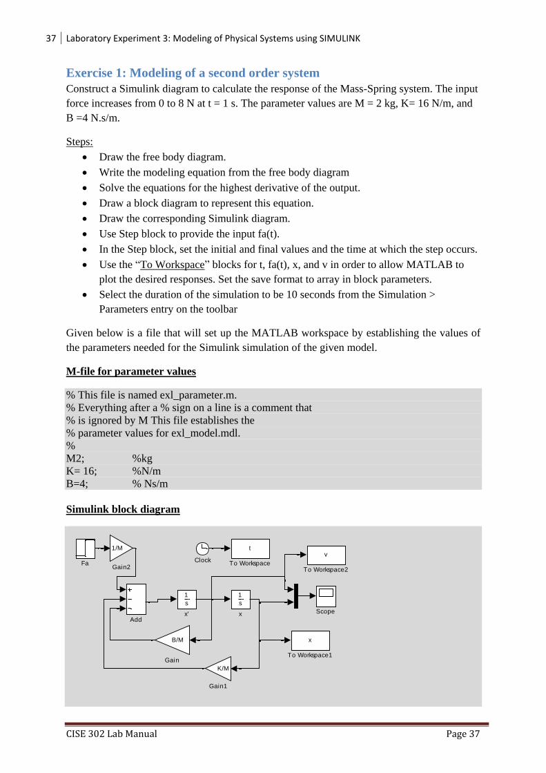
Exercise 1: Modeling of a second order system
Construct a Simulink diagram to calculate the response of the Mass-Spring system. The input
force increases from 0 to 8 N at t = 1 s. The parameter values are M = 2 kg, K= 16 N/m, and
B =4 N.s/m.
Steps:
Draw the free body diagram.
Write the modeling equation from the free body diagram
Solve the equations for the highest derivative of the output.
Draw a block diagram to represent this equation.
Draw the corresponding Simulink diagram.
Use Step block to provide the input fa(t).
In the Step block, set the initial and final values and the time at which the step occurs.
Use the “To Workspace” blocks for t, fa(t), x, and v in order to allow MATLAB to
plot the desired responses. Set the save format to array in block parameters.
Select the duration of the simulation to be 10 seconds from the Simulation >
Parameters entry on the toolbar
Given below is a file that will set up the MATLAB workspace by establishing the values of
the parameters needed for the Simulink simulation of the given model.
M-file for parameter values
% This file is named exl_parameter.m.
% Everything after a % sign on a line is a comment that
% is ignored by M This file establishes the
% parameter values for exl_model.mdl.
%
M2; %kg
K= 16; %N/m
B=4; % Ns/m
Simulink block diagram
1
s
x'
1
s
x
v
To Workspace2
x
To Workspace1
t
To Workspace
Scope
1/M
Gain2
K/M
Gain1
B/M
Gain
FaClock
Add
38 Laboratory Experiment 3: Modeling of Physical Systems using SIMULINK
CISE 302 Lab Manual Page 38
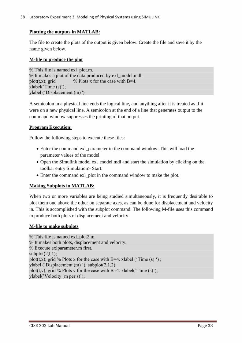
Plotting the outputs in MATLAB:
The file to create the plots of the output is given below. Create the file and save it by the
name given below.
M-file to produce the plot
% This file is named exl_plot.m.
% It makes a plot of the data produced by exl_model.mdl.
plot(t,x); grid % Plots x for the case with B=4.
xlabel(’Time (s)’);
ylabel (‘Displacement (m) ')
A semicolon in a physical line ends the logical line, and anything after it is treated as if it
were on a new physical line. A semicolon at the end of a line that generates output to the
command window suppresses the printing of that output.
Program Execution:
Follow the following steps to execute these files:
Enter the command exl_parameter in the command window. This will load the
parameter values of the model.
Open the Simulink model exl_model.mdl and start the simulation by clicking on the
toolbar entry Simulation> Start.
Enter the command exl_plot in the command window to make the plot.
Making Subplots in MATLAB:
When two or more variables are being studied simultaneously, it is frequently desirable to
plot them one above the other on separate axes, as can be done for displacement and velocity
in. This is accomplished with the subplot command. The following M-file uses this command
to produce both plots of displacement and velocity.
M-file to make subplots
% This file is named exl_plot2.m.
% It makes both plots, displacement and velocity.
% Execute exlparameter.m first.
subplot(2,l,1);
plot(t,x); grid % Plots x for the case with B=4. xlabel (‘Time (s) ‘) ;
ylabel (‘Displacement (m) ‘); subplot(2,1,2);
plot(t,v); grid % Plots v for the case with B=4. xlabel(’Time (s)’);
ylabel(’Velocity (m per s)’);

39 Laboratory Experiment 3: Modeling of Physical Systems using SIMULINK
CISE 302 Lab Manual Page 39
Exercise 2: Simulation with system parameter variation
The effect of changing B is to alter the amount of overshoot or undershoot. These are related
to a term called the damping ratio. Simulate and compare the results of the variations in B in
exercise 1. Take values of B = 4, 8, 12, 25 N-s/m.
Steps:
Perform the following steps. Use the same input force as in Exercise 1.
Begin the simulation with B = 4 N-s/m, but with the input applied at t = 0
Plot the result.
Rerun it with B = 8 N.s/m.
Hold the first plot active, by the command hold on
Reissue the plot command plot(t,x), the second plot will superimpose on the first.
Repeat for B = 12 N-s/m and for B = 25 N-s/m
Release the plot by the command hold off
Show your result.
Running SIMULINK from MATLAB command prompt
If a complex plot is desired, in which several runs are needed with different parameters, this
can using the command called “sim”. “sim” command will run the Simulink model file from
the Matlab command prompt. For multiple runs with several plot it can be accomplished by
executing ex1_model (to load parameters) followed by given M-file. Entering the command
ex1_plots in the command window results in multiple runs with varying values if B and will
plot the results.
M-file to use “sim” function and produce multiple runs and their plots
% This file is named ex2_plots.m.
% It plots the data produced by exl_model.mdl for
% several values of B. Execute exl_parameter.m first.
sim(’exl_model’) % Has the same effect as clicking on
% Start on the toolbar.
plot(t,x) % Plots the initial run with B=4
hold on % Plots later results on the same axes % as the first.
B = 8; % New value of B; other parameter values % stay the same.
sim(‘exl_model’) % Rerun the simulation with new B value.
plot(t,x) % Plots new x on original axes.
B 12; sim(’exl_model’);plot(t,x)
B = 25; sim(’exl_model’ ) ;plot(t,x)
hold off

40 Laboratory Experiment 3: Modeling of Physical Systems using SIMULINK
CISE 302 Lab Manual Page 40
Exercise 3: System response from the stored energy with zero input
Find the response of the above system when there is no input for t ≥0, but when the initial
value of the displacement x(0) is zero and the initial velocity v(0) is 1 m/s.
Steps:
In the previous program
Set the size of the input step to zero
Set the initial condition on Integrator for velocity to 1.0.
Plot the results by running m-files.
Exercise 4: Cruise System
As we know in the cruise system, the spring force ( ) which means that K=0.
Equation (2) becomes
( )
( )
( ) (3)
Or
( )
( ) (4)
Find the velocity response of the above system by constructing a Simulink block diagram
and calling the block diagram from Matlab m-file. Use M=750, B=30 and a constant force Fa
= 300. Plot the response of the system such that it runs for 125 seconds.
41 Laboratory Experiment 4: Linear Time-invariant Systems and Representation
CISE 302 Lab Manual Page 41
CISE 302
Linear Control Systems
Laboratory Experiment 4: Linear Time-invariant Systems and
Representation
Objectives: This experiment has following two objectives:
1. Continued with the learning of Mathematical Modeling from previous experiment, we
now start focusing the linear systems. We will learn commands in MATLAB that
would be used to represent such systems in terms of transfer function or pole-zero-
gain representations.
2. We will also learn how to make preliminary analysis of such systems using plots of
poles and zeros locations as well as time response due to impulse, step and arbitrary
inputs.
List of Equipment/Software
Following equipment/software is required:
MATLAB
Category Soft-Experiment
Deliverables
A complete lab report including the following:
Summarized learning outcomes.
MATLAB scripts and their results should be reported properly.
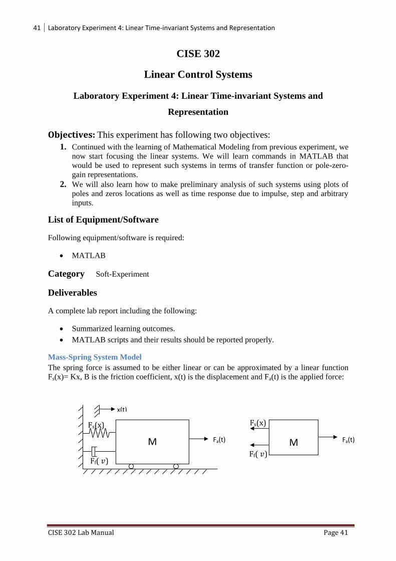
Mass-Spring System Model
The spring force is assumed to be either linear or can be approximated by a linear function
Fs(x)= Kx, B is the friction coefficient, x(t) is the displacement and Fa(t) is the applied force:
Fs(x)
M
Ff( 𝑣)
Fa(t)
x(t)
M Fa(t)
Ff( 𝑣)
Fs(x)

42 Laboratory Experiment 4: Linear Time-invariant Systems and Representation
CISE 302 Lab Manual Page 42
The differential equation for the above Mass-Spring system can be derived as follows
( )
( )
( ) ( )
Transfer Function:
Applying the Laplace transformation while assuming the initial conditions are zeros, we get
( ) ( ) ( )
Then the transfer function representation of the system is given by
( )
( )
( )
Linear Time-Invariant Systems in MATLAB:
Control System Toolbox in MATLAB offers extensive tools to manipulate and analyze linear
time-invariant (LTI) models. It supports both continuous- and discrete-time systems. Systems
can be single-input/single-output (SISO) or multiple-input/multiple-output (MIMO). You can
specify LTI models as:
Transfer functions (TF), for example,
( )
Note: All LTI models are represented as a ratio of polynomial functions
Examples of Creating LTI Models
Building LTI models with Control System Toolbox is straightforward. The following sections
show simple examples. Note that all LTI models, i.e. TF, ZPK and SS are also MATLAB
objects.
Example of Creating Transfer Function Models
You can create transfer function (TF) models by specifying numerator and denominator
coefficients. For example,
>>num = [1 0];
>>den = [1 2 1];
>>sys = tf(num,den)
Transfer function:
s
-------------
s^2 + 2 s + 1
A useful trick is to create the Laplace variable, s. That way, you can specify polynomials
using s as the polynomial variable.
>>s=tf('s');
>>sys= s/(s^2 + 2*s + 1)

43 Laboratory Experiment 4: Linear Time-invariant Systems and Representation
CISE 302 Lab Manual Page 43
Transfer function:
s
-------------
s^2 + 2 s + 1
This is identical to the previous transfer function.
Example of Creating Zero-Pole-Gain Models
To create zero-pole-gain (ZPK) models, you must specify each of the three components in
vector format. For example,
>>sys = zpk([0],[-1 -1],[1])
Zero/pole/gain:
s
-------
(s+1)^2
produces the same transfer function built in the TF example, but the representation is now
ZPK. This example shows a more complicated ZPK model.
>>sys=zpk([1 0], [-1 -3 -.28],[.776])
Zero/pole/gain:
0.776 s (s-1)
--------------------
(s+1) (s+3) (s+0.28)
Plotting poles and zeros of a system:
pzmap
Compute pole-zero map of LTI models
pzmap(sys)
pzmap(sys1,sys2,...,sysN)
[p,z] = pzmap(sys)
Description:
pzmap(sys) plots the pole-zero map of the
continuous- or discrete-time LTI model sys. For
SISO systems, pzmap plots the transfer function
poles and zeros. The poles are plotted as x's and the
zeros are plotted as o's.
pzmap(sys1,sys2,...,sysN) plots the pole-zero map
of several LTI models on a single figure. The LTI
models can have different numbers of inputs and
outputs. When invoked with left-hand arguments,
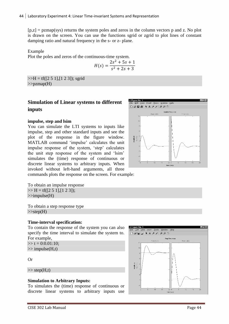
44 Laboratory Experiment 4: Linear Time-invariant Systems and Representation
CISE 302 Lab Manual Page 44
[p,z] = pzmap(sys) returns the system poles and zeros in the column vectors p and z. No plot
is drawn on the screen. You can use the functions sgrid or zgrid to plot lines of constant
damping ratio and natural frequency in the s- or z- plane.
Example
Plot the poles and zeros of the continuous-time system.
( )
>>H = tf([2 5 1],[1 2 3]); sgrid
>>pzmap(H)
Simulation of Linear systems to different
inputs
impulse, step and lsim
You can simulate the LTI systems to inputs like
impulse, step and other standard inputs and see the
plot of the response in the figure window.
MATLAB command ‘impulse’ calculates the unit
impulse response of the system, ‘step’ calculates
the unit step response of the system and ‘lsim’
simulates the (time) response of continuous or
discrete linear systems to arbitrary inputs. When
invoked without left-hand arguments, all three
commands plots the response on the screen. For example:
To obtain an impulse response
>> H = tf([2 5 1],[1 2 3]);
>>impulse(H)
To obtain a step response type
>>step(H)
Time-interval specification:
To contain the response of the system you can also
specify the time interval to simulate the system to.
For example,
>> t = 0:0.01:10;
>> impulse(H,t)
Or
>> step(H,t)
Simulation to Arbitrary Inputs:
To simulates the (time) response of continuous or
discrete linear systems to arbitrary inputs use
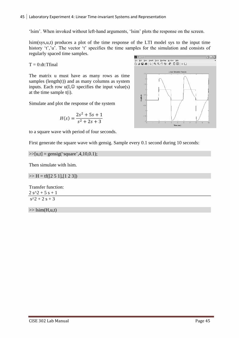
45 Laboratory Experiment 4: Linear Time-invariant Systems and Representation
CISE 302 Lab Manual Page 45
‘lsim’. When invoked without left-hand arguments, ‘lsim’ plots the response on the screen.
lsim(sys,u,t) produces a plot of the time response of the LTI model sys to the input time
history ‘t’,’u’. The vector ‘t’ specifies the time samples for the simulation and consists of
regularly spaced time samples.
T = 0:dt:Tfinal
The matrix u must have as many rows as time
samples (length(t)) and as many columns as system
inputs. Each row u(I, specifies the input value(s)
at the time sample t(i).
Simulate and plot the response of the system
( )
to a square wave with period of four seconds.
First generate the square wave with gensig. Sample every 0.1 second during 10 seconds:
>>[u,t] = gensig(‘square’,4,10,0.1);
Then simulate with lsim.
>> H = tf([2 5 1],[1 2 3])
Transfer function:
2 s^2 + 5 s + 1
s^2 + 2 s + 3
>> lsim(H,u,t)

46 Laboratory Experiment 4: Linear Time-invariant Systems and Representation
CISE 302 Lab Manual Page 46
Exercise 1:
Consider the transfer function
( )
Using MATLAB plot the pole zero map of the above system
Exercise 2:
a. Obtain the unit impulse response for the following system
( )
( )
b. Obtain the unit step response for the following system
( )
( )
c. Explain why the results in a. and b. are same?
Exercise 3:
A system has a transfer function
( )
( ) ( ⁄ )( )
Plot the response of the system when R(s) is a unit impulse and unit step for the
parameter z=3, 6 and 12.
Exercise 4:
Consider the differential equation where ( ) ( ) and
( ) is a unit step. Determine the solution analytically and verify by co-plotting the
analytical solution and the step response obtained with ‘step’ function.

47 Lab Experiment 5: Block Diagram Reduction
CISE 302 Lab Manual Page 47
CISE 302
Linear Control Systems
Lab Experiment 5: Block Diagram Reduction
Objective: The objective of this exercise will be to learn commands in MATLAB that
would be used to reduce linear systems block diagram using series, parallel and feedback
configuration.
List of Equipment/Software
Following equipment/software is required:
MATLAB
Category Soft-Experiment
Deliverables
A complete lab report including the following:
Summarized learning outcomes.
MATLAB scripts and their results for examples, exercises and Dorf (text book)
related material of this lab should be reported properly.
Series configuration: If the two blocks are connected as shown below then the blocks are
said to be in series. It would like multiplying two transfer functions. The MATLAB
command for the such configuration is “series”.
The series command is implemented as shown below:
Example 1: Given the transfer functions of individual blocks generate the system transfer
function of the block combinations.
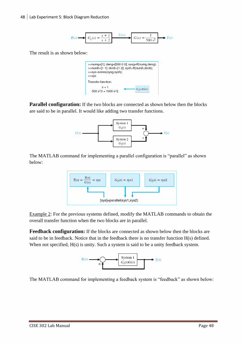
48 Lab Experiment 5: Block Diagram Reduction
CISE 302 Lab Manual Page 48
The result is as shown below:
Parallel configuration: If the two blocks are connected as shown below then the blocks
are said to be in parallel. It would like adding two transfer functions.
The MATLAB command for implementing a parallel configuration is “parallel” as shown
below:
Example 2: For the previous systems defined, modify the MATLAB commands to obtain the
overall transfer function when the two blocks are in parallel.
Feedback configuration: If the blocks are connected as shown below then the blocks are
said to be in feedback. Notice that in the feedback there is no transfer function H(s) defined.
When not specified, H(s) is unity. Such a system is said to be a unity feedback system.
The MATLAB command for implementing a feedback system is “feedback” as shown below:
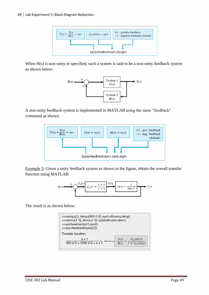
49 Lab Experiment 5: Block Diagram Reduction
CISE 302 Lab Manual Page 49
When H(s) is non-unity or specified, such a system is said to be a non-unity feedback system
as shown below:
A non-unity feedback system is implemented in MATLAB using the same “feedback”
command as shown:
Example 3: Given a unity feedback system as shown in the figure, obtain the overall transfer
function using MATLAB:
The result is as shown below:
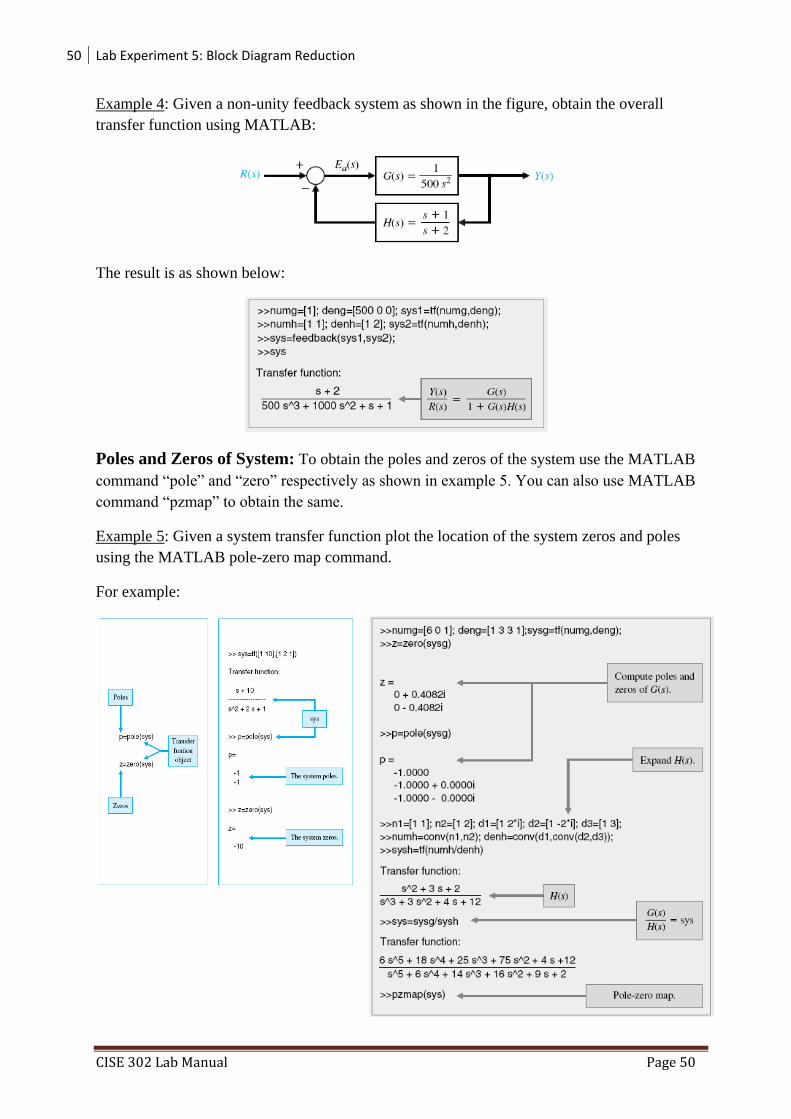
50 Lab Experiment 5: Block Diagram Reduction
CISE 302 Lab Manual Page 50
Example 4: Given a non-unity feedback system as shown in the figure, obtain the overall
transfer function using MATLAB:
The result is as shown below:
Poles and Zeros of System: To obtain the poles and zeros of the system use the MATLAB
command “pole” and “zero” respectively as shown in example 5. You can also use MATLAB
command “pzmap” to obtain the same.
Example 5: Given a system transfer function plot the location of the system zeros and poles
using the MATLAB pole-zero map command.
For example:

51 Lab Experiment 5: Block Diagram Reduction
CISE 302 Lab Manual Page 51
Exercise 1: For the following multi-loop feedback system, get closed loop transfer function
and the corresponding pole-zero map of the system.
Given )10(
11
sG ;
)1(
12
sG ;
)44(
12
2
3
ss
sG ;
)6(
14
s
sG ;
)2(
11
s
sH ; 22 H
; 13 H (Reference: Page 113, Chapter 2, Text: Dorf.)
MATLAB solution:
Instruction: Please refer to Section 2.6 and Section 2.2 in Text by Dorf.
Exercise 2: Consider the feedback system depicted in the figure below
a. Compute the closed-loop transfer function using the ‘series’ and ‘feedback’ functions
b. Obtain the closed-loop system unit step response with the ‘step’ function and verify
that final value of the output is 2/5.
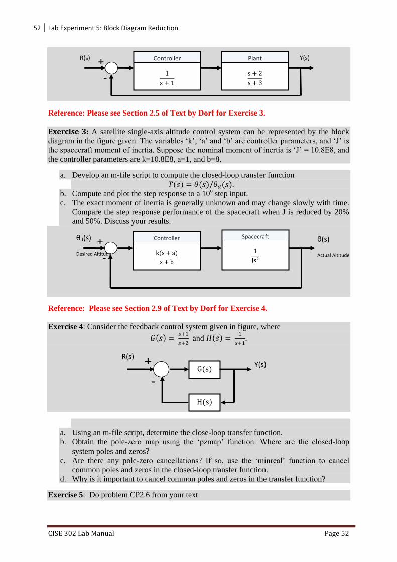
52 Lab Experiment 5: Block Diagram Reduction
CISE 302 Lab Manual Page 52
Reference: Please see Section 2.5 of Text by Dorf for Exercise 3.
Exercise 3: A satellite single-axis altitude control system can be represented by the block
diagram in the figure given. The variables ‘k’, ‘a’ and ‘b’ are controller parameters, and ‘J’ is
the spacecraft moment of inertia. Suppose the nominal moment of inertia is ‘J’ = 10.8E8, and
the controller parameters are k=10.8E8, a=1, and b=8.
a. Develop an m-file script to compute the closed-loop transfer function
( ) ( ) ( ). b. Compute and plot the step response to a 10
o step input.
c. The exact moment of inertia is generally unknown and may change slowly with time.
Compare the step response performance of the spacecraft when J is reduced by 20%
and 50%. Discuss your results.
Reference: Please see Section 2.9 of Text by Dorf for Exercise 4.
Exercise 4: Consider the feedback control system given in figure, where
( )
and ( )
.
a. Using an m-file script, determine the close-loop transfer function.
b. Obtain the pole-zero map using the ‘pzmap’ function. Where are the closed-loop
system poles and zeros?
c. Are there any pole-zero cancellations? If so, use the ‘minreal’ function to cancel
common poles and zeros in the closed-loop transfer function.
d. Why is it important to cancel common poles and zeros in the transfer function?
Exercise 5: Do problem CP2.6 from your text
s
Controller
s
s
Plant
-
+ R(s) Y(s)
k(s a)
s b
Controller
Js
Spacecraft
-
+
G(s)
-
+ R(s) Y(s)
H(s)
θ(s)
Actual Altitude
θd(s)
Desired Altitude

53 Lab Experiment 6: Performance of First order and second order systems
CISE 302 Lab Manual Page 53
CISE 302
Linear Control Systems
Lab Experiment 6: Performance of First order and second order systems
Objective: The objective of this exercise will be to study the performance characteristics of
first and second order systems using MATLAB.
List of Equipment/Software
Following equipment/software is required:
MATLAB
Category Soft-Experiment
Deliverables
A complete lab report including the following:
Summarized learning outcomes.
MATLAB scripts and their results for Exercise 1 & 2 should be reported properly.
Overview First Order Systems:
An electrical RC-circuit is the simplest example of a first order system. It comprises of a
resistor and capacitor connected in series to a voltage supply as shown below on Figure 1.
Figure 1: RC Circuit
If the capacitor is initially uncharged at zero voltage when the circuit is switched on, it starts
to charge due to the current ‘i' through the resistor until the voltage across it reaches the
supply voltage. As soon as this happens, the current stops flowing or decays to zero, and the
circuit becomes like an open circuit. However, if the supply voltage is removed, and the
circuit is closed, the capacitor will discharge the energy it stored again through the resistor.
The time it takes the capacitor to charge depends on the time constant of the system, which is
defined as the time taken by the voltage across the capacitor to rise to approximately 63% of
the supply voltage. For a given RC-circuit, this time constant is . Hence its magnitude
depends on the values of the circuit components.
+
-
R
C E(t) Vc(t)

54 Lab Experiment 6: Performance of First order and second order systems
CISE 302 Lab Manual Page 54
The RC circuit will always behave in this way, no matter what the values of the components.
That is, the voltage across the capacitor will never increase indefinitely. In this respect we
will say that the system is passive and because of this property it is stable.
For the RC-circuit as shown in Fig. 1, the equation governing its behavior is given by
( )
( )
where ( ) (1)
where ( ) is the voltage across the capacitor, R is the resistance and C is the capacitance.
The constant is the time constant of the system and is defined as the time required by
the system output i.e. ( ) to rise to 63% of its final value (which is E). Hence the above
equation (1) can be expressed in terms of the time constant as:
( )
( ) where ( ) (1)
Obtaining the transfer function of the above differential equation, we get
( )
( )
(2)
where τ is time constant of the system and the system is known as the first order system. The
performance measures of a first order system are its time constant and its steady state.
Exercise 1:
a) Given the values of R and C, obtain the unit step response of the first order system.
a. R=2KΩ and C=0.01F
b. R=2.5KΩ and C=0.003F
b) Verify in each case that the calculated time constant ( ) and the one measured
from the figure as 63% of the final value are same.
c) Obtain the steady state value of the system.
Overview Second Order Systems:
Consider the following Mass-Spring system shown in the Figure 2. Where K is the spring
constant, B is the friction coefficient, x(t) is the displacement and F(t) is the applied force:
Figure 2. Mass-Spring system
The differential equation for the above Mass-Spring system can be derived as follows
( )
( )
( ) ( )
K
M
B
F(t)
x(t)

55 Lab Experiment 6: Performance of First order and second order systems
CISE 302 Lab Manual Page 55
Applying the Laplace transformation we get
( ) ( ) ( )
provided that, all the initial conditions are zeros. Then the transfer function representation of
the system is given by
( )
( )
( )
The above system is known as a second order system.
The generalized notation for a second order system described above can be written as
2
2 2( ) ( )
2
n
n n
Y s R ss s
With the step input applied to the system, we obtain
2
2 2( )
( 2 )
n
n n
Y ss s s
for which the transient output, as obtained from the Laplace transform table (Table 2.3,
Textbook), is
2 1
2
1( ) 1 sin( 1 cos ( ))
1
nt
ny t e t
where 0 < ζ < 1. The transient response of the system changes for different values of damping
ratio, ζ. Standard performance measures for a second order feedback system are defined in
terms of step response of a system. Where, the response of the second order system is shown
below.

56 Lab Experiment 6: Performance of First order and second order systems
CISE 302 Lab Manual Page 56
The performance measures could be described as follows:
Rise Time: The time for a system to respond to a step input and attains a response equal to a
percentage of the magnitude of the input. The 0-100% rise time, Tr, measures the time to
100% of the magnitude of the input. Alternatively, Tr1, measures the time from 10% to 90%
of the response to the step input.
Peak Time: The time for a system to respond to a step input and rise to peak response.
Overshoot: The amount by which the system output response proceeds beyond the desired
response. It is calculated as
P.O.= 100%tpM f
f
where MPt is the peak value of the time response, and fv is the final value of the response.
Settling Time: The time required for the system’s output to settle within a certain percentage
of the input amplitude (which is usually taken as 2%). Then, settling time, Ts, is calculated as
4s
n
T
Exercise 2: Effect of damping ratio ζ on performance measures. For a single-loop second
order feedback system given below
Find the step response of the system for values of ωn = 1 and ζ = 0.1, 0.4, 0.7, 1.0 and 2.0.
Plot all the results in the same figure window and fill the following table.
ζ Rise time Peak Time % Overshoot Settling time Steady state value
0.1
0.4
0.7
1.0
2.0
R(s) E(s)
Y(s) +
-

57 Lab Experiment 7: DC Motor Characteristics
CISE 302 Lab Manual Page 57
CISE 302
Linear Control Systems
Lab Experiment 7: DC Motor Characteristics
Objective: The objective of the experiment is to show how a permanent magnet D.C.
motor may be controlled by varying the magnitude and direction of its armature current and
recognize the torque/speed characteristic of the D.C. Motor
List of Equipment/Software
Following equipment/software is required:
MATLAB
LabVIEW
DC Servo System (feedback equipment)
a. OU150A Op Amp Unit
b. AU150B Attenuator Unit
c. PA150C Pre-Amplifier Unit
d. SA150D Servo Amplifier
e. PS150E Power Supply
f. DCM150F DC Motor
g. IP150H Input Potentiometer
h. OP150K Output Potentiometer
i. GT150X Reduction Gear Tacho
j. DC Voltmeter
Category Software-Hardware Experiment
Note: This lab exercise may take two weeks.
Deliverables
A complete lab report including the following:
Summarized learning outcomes.
Clearly show the model development and the Simulink model.
Show the parameter identification graphs and calculations properly.
Connection diagram of the hardware experimental part.
Report the results in the table and graphical way with summarized learning outcomes.
Introduction:
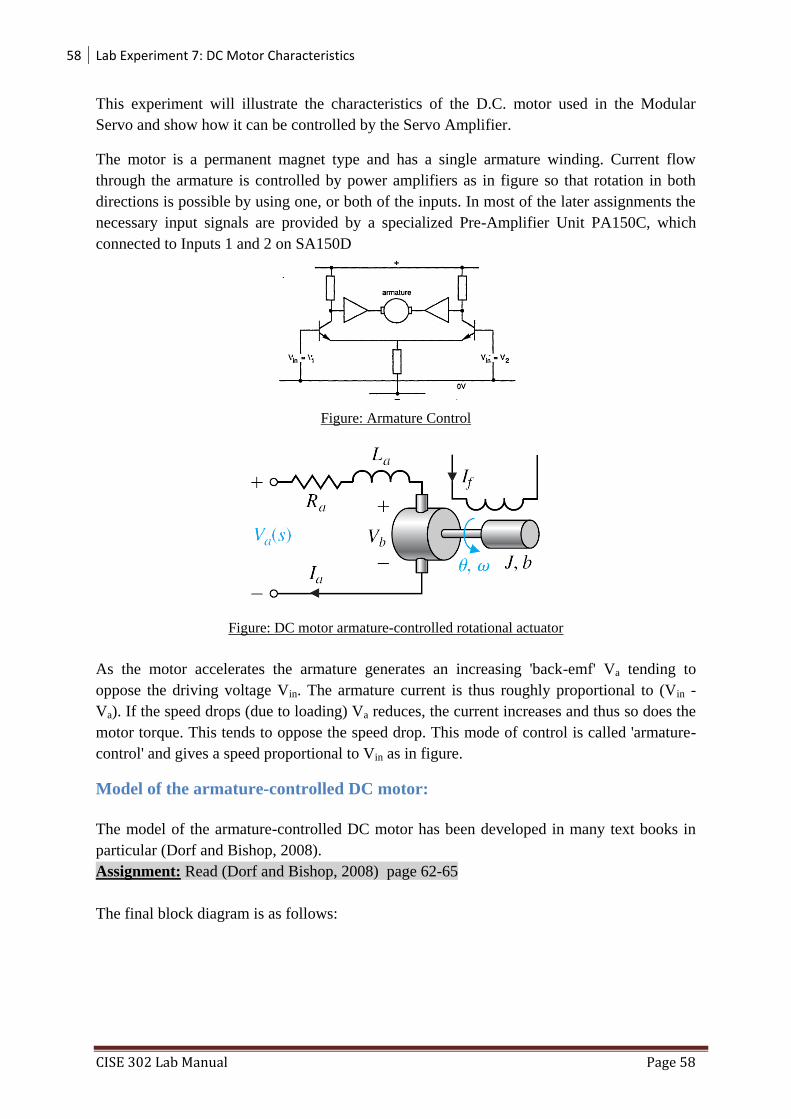
58 Lab Experiment 7: DC Motor Characteristics
CISE 302 Lab Manual Page 58
This experiment will illustrate the characteristics of the D.C. motor used in the Modular
Servo and show how it can be controlled by the Servo Amplifier.
The motor is a permanent magnet type and has a single armature winding. Current flow
through the armature is controlled by power amplifiers as in figure so that rotation in both
directions is possible by using one, or both of the inputs. In most of the later assignments the
necessary input signals are provided by a specialized Pre-Amplifier Unit PA150C, which
connected to Inputs 1 and 2 on SA150D
Figure: Armature Control
Figure: DC motor armature-controlled rotational actuator
As the motor accelerates the armature generates an increasing 'back-emf' Va tending to
oppose the driving voltage Vin. The armature current is thus roughly proportional to (Vin -
Va). If the speed drops (due to loading) Va reduces, the current increases and thus so does the
motor torque. This tends to oppose the speed drop. This mode of control is called 'armature-
control' and gives a speed proportional to Vin as in figure.
Model of the armature-controlled DC motor:
The model of the armature-controlled DC motor has been developed in many text books in
particular (Dorf and Bishop, 2008).
Assignment: Read (Dorf and Bishop, 2008) page 62-65
The final block diagram is as follows:

59 Lab Experiment 7: DC Motor Characteristics
CISE 302 Lab Manual Page 59
Model Simulation using Simulink:
Prerequisite to this section is a mathematical understanding of the elctro-mechanical model
of a DC motor. Student should be able to understand how electrical terms (voltage, current,
emf) interact with mechanical terms (speed, position) via electro-magnetic circuit
(inductance). The students should be able to understand and derive the mathematical model
of a DC motor.
The motor torque, T, is related to the armature current, i, by a constant factor Kt. The back
emf, e, is related to the rotational velocity by the following equations:
iKT t
dt
dKe e
In SI units (which we will use), Kt (armature constant) is equal to Ke (motor constant).
1. Building the Model
This system will be modeled by summing the torques acting on the rotor inertia and
integrating the acceleration to give the velocity, and integrating velocity to get position. Also,
Kirchoff's laws will be applied to the armature circuit.
Open Simulink and open a new model window. First, we will model the integrals of the
rotational acceleration and of the rate of change of armature current.
dt
d
dt
d2
2
idt
di
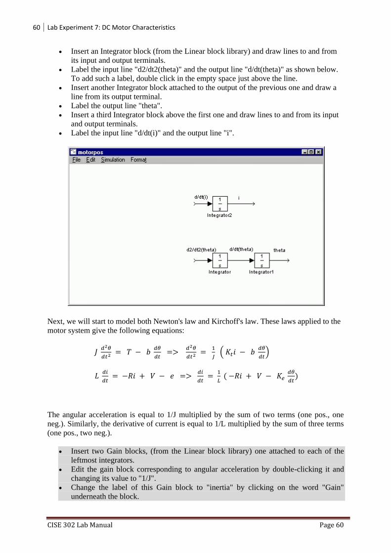
60 Lab Experiment 7: DC Motor Characteristics
CISE 302 Lab Manual Page 60
Insert an Integrator block (from the Linear block library) and draw lines to and from
its input and output terminals.
Label the input line "d2/dt2(theta)" and the output line "d/dt(theta)" as shown below.
To add such a label, double click in the empty space just above the line.
Insert another Integrator block attached to the output of the previous one and draw a
line from its output terminal.
Label the output line "theta".
Insert a third Integrator block above the first one and draw lines to and from its input
and output terminals.
Label the input line "d/dt(i)" and the output line "i".
Next, we will start to model both Newton's law and Kirchoff's law. These laws applied to the
motor system give the following equations:
(
)
(
)
The angular acceleration is equal to 1/J multiplied by the sum of two terms (one pos., one
neg.). Similarly, the derivative of current is equal to 1/L multiplied by the sum of three terms
(one pos., two neg.).
Insert two Gain blocks, (from the Linear block library) one attached to each of the
leftmost integrators.
Edit the gain block corresponding to angular acceleration by double-clicking it and
changing its value to "1/J".
Change the label of this Gain block to "inertia" by clicking on the word "Gain"
underneath the block.
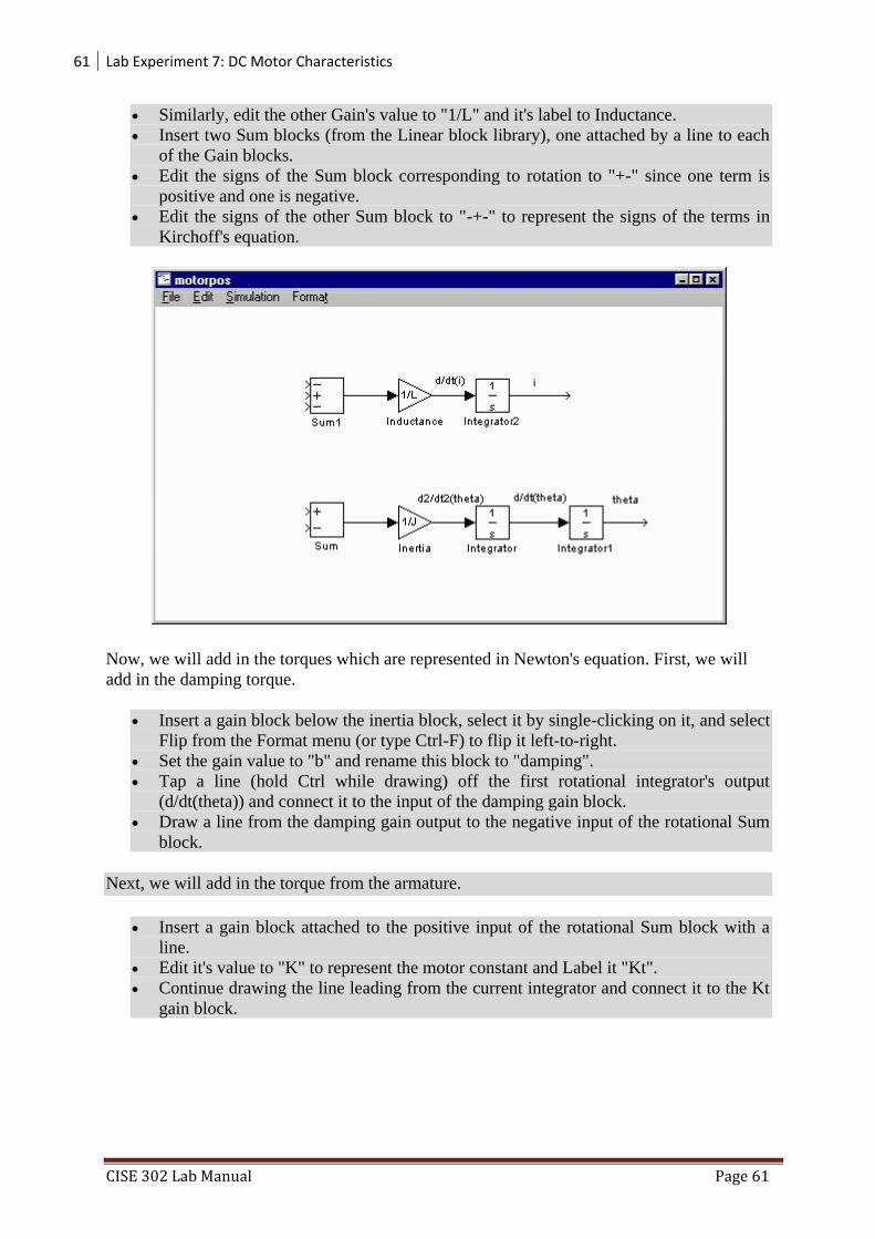
61 Lab Experiment 7: DC Motor Characteristics
CISE 302 Lab Manual Page 61
Similarly, edit the other Gain's value to "1/L" and it's label to Inductance.
Insert two Sum blocks (from the Linear block library), one attached by a line to each
of the Gain blocks.
Edit the signs of the Sum block corresponding to rotation to "+-" since one term is
positive and one is negative.
Edit the signs of the other Sum block to "-+-" to represent the signs of the terms in
Kirchoff's equation.
Now, we will add in the torques which are represented in Newton's equation. First, we will
add in the damping torque.
Insert a gain block below the inertia block, select it by single-clicking on it, and select
Flip from the Format menu (or type Ctrl-F) to flip it left-to-right.
Set the gain value to "b" and rename this block to "damping".
Tap a line (hold Ctrl while drawing) off the first rotational integrator's output
(d/dt(theta)) and connect it to the input of the damping gain block.
Draw a line from the damping gain output to the negative input of the rotational Sum
block.
Next, we will add in the torque from the armature.
Insert a gain block attached to the positive input of the rotational Sum block with a
line.
Edit it's value to "K" to represent the motor constant and Label it "Kt".
Continue drawing the line leading from the current integrator and connect it to the Kt
gain block.

62 Lab Experiment 7: DC Motor Characteristics
CISE 302 Lab Manual Page 62
Now, we will add in the voltage terms which are represented in Kirchoff's equation. First, we
will add in the voltage drop across the coil resistance.
Insert a gain block above the inductance block, and flip it left-to-right.
Set the gain value to "R" and rename this block to "Resistance".
Tap a line (hold Ctrl while drawing) off the current integrator's output and connect it
to the input of the resistance gain block.
Draw a line from the resistance gain output to the upper negative input of the current
equation Sum block.
Next, we will add in the back emf from the motor.
Insert a gain block attached to the other negative input of the current Sum block with
a line.
Edit it's value to "K" to represent the motor constant and Label it "Ke".
Tap a line off the first rotational integrator's output (d/dt(theta)) and connect it to the
Ke gain block.

63 Lab Experiment 7: DC Motor Characteristics
CISE 302 Lab Manual Page 63
The third voltage term in the Kirchoff equation is the control input, V. We will apply a step
input.
Insert a Step block (from the Sources block library) and connect it with a line to the
positive input of the current Sum block.
To view the output speed, insert a Scope (from the Sinks block library) connected to
the output of the second rotational integrator (theta).
To provide a appropriate unit step input at t=0, double-click the Step block and set the
Step Time to "0".
2. DC motor nominal values

64 Lab Experiment 7: DC Motor Characteristics
CISE 302 Lab Manual Page 64
moment of inertia of the rotor (J) = 3.2284E-6 kg.m^2/s^2
damping ratio of the mechanical system (b) = 3.5077E-6 Nms
electromotive force constant (K=Ke=Kt) = 0.0274 Nm/Amp
electric resistance (R) = 4 ohm
electric inductance (L) = 2.75E-6 H
input (V): Source Voltage
output (theta): position of shaft
Assumption: The rotor and shaft are assumed to be rigid
The physical parameters must now be set. Run the following commands at the MATLAB
prompt:
J=3.2284E-6;
b=3.5077E-6;
K=0.0274;
R=4;
L=2.75E-6;
Run the simulation (Ctrl-t or Start on the Simulation menu).
3. Simulation:
To simulate this system, first, an appropriate simulation time must be set. Select Parameters
from the Simulation menu and enter "0.2" in the Stop Time field. 0.2 seconds is long enough
to view the open-loop response. Also in the Parameters dialog box, it is helpful to change the
Solver Options method. Click on the field which currently contains "ode45 (Dormand-
Prince)". Select the option "ode15s (stiff/NDF)". Since the time scales in this example are
very small, this stiff system integration method is much more efficient than the default
integration method.
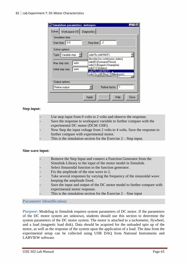
65 Lab Experiment 7: DC Motor Characteristics
CISE 302 Lab Manual Page 65
Step input:
- Use step input from 0 volts to 2 volts and observe the response.
- Save the response to workspace variable to further compare with the
experimental DC motor (DCM 150F).
- Now Step the input voltage from 2 volts to 4 volts. Save the response to
further compare with experimental motor.
- This is the simulation section for the Exercise 2 – Step input.
Sine wave input:
- Remove the Step Input and connect a Function Generator from the
Simulink-Library to the input of the motor model in Simulink.
- Select Sinusoidal function in the function generator.
- Fix the amplitude of the sine wave to 2.
- Take several responses by varying the frequency of the sinusoidal wave
keeping the amplitude fixed.
- Save the input and output of the DC motor model to further compare with
experimental motor response.
- This is the simulation section for the Exercise 2 – Sine input
Parameter Identification:
Purpose: Modeling in Simulink requires system parameters of DC motor. If the parameters
of the DC motor system are unknown, students should use this section to determine the
system parameters of the DC motor system. The motor is attached to a tachometer, flywheel,
and a load (magnetic load disk). Data should be acquired for the unloaded spin up of the
motor, as well as the response of the system upon the application of a load. The data from the
experimental setup can be collected using USB DAQ from National Instruments and
LABVIEW software.

66 Lab Experiment 7: DC Motor Characteristics
CISE 302 Lab Manual Page 66
Derivations
To measure the constants km and R, we can use equations following equations,
mm ke
R
eei maa
Divide by ae ,
Hint: The last equation resembles with the well known cmxy equation of a line.
Since we have measured values for ae , ai , and , we can plot a
a
i
eversus
ai
to determine the
slope and intercept, which reveals the constant values of mk and R .
To derive B , ft , and wk we use the equation
faim BJik
For steady state 0
, so we have
fm B
If we plot the graph of m and , and plot a best fit line, we can get the corresponding values
of B and f .
Once we know m , we can find ik using
aim ik
a
m
a
a
eR
k
Re
i
1
Re
i
eR
k
a
a
a
m 1
Re
i
eR
iRk
a
a
a
am 1
RiRk
eR
am
a
ama iRke
Rkii
em
aa
a
67 Lab Experiment 7: DC Motor Characteristics
CISE 302 Lab Manual Page 67
Note that k is the slope of the te vs graph.
Summarize the system parameters for the DC motor in corresponding graphs and tables. Use
these parameters in the Simulink Model simulation and validate the Simulation results with
the experimental set up.
Viscous Friction vs. Coulomb Friction
We can estimate the speed at which the viscous friction is greater than the coulomb friction,
that is, when fTB . The speed can be calculated by dividing fT by B .
The approximate tachometer voltage corresponding to this speed can be determined by using
the best fit equation for the relationship between te and .
After determining the best fit equation for te and , we can plug in the value of calculated
above to get an expected tachometer voltage te .
Note that the voltage estimated may be greater than the tachometer voltage determined by the
experimental setup in lab. This case, we can assume that the Coulomb friction in the motor
system dominates.
Calculating J from the Motor Spinup Data
Applying a step input of to the motor and acquiring data samples, we can obtain a curve for
the tachometer voltage vs. time. Given the form of the first order response of the system to an
input, we can further fit the data with an appropriate exponential to determine the time
constant.
)1(1
.)(.1
)(
)()( at
t
a
t ea
Kteas
K
ssE
sEsFunctionTransfer
Where,
JR
kkBRa im
1, and
JR
kkK i
Using the above equations and the best fit constants for the motor spin up obtained above, we
can calculate the value of J .
Figures to be plotted:
1. te (volts) versus )/( srad : To determine k .
2. a
a
i
e(volts/ampere = ohms) versus
ai
(rad/(sec*Amp)): To determine constants mk and
.R
3. mT (N*m) versus (rad/s): To determine B and fT .
Table of values: Tfm kTkRBk

68 Lab Experiment 8: Validation of DC Motor Characteristics
CISE 302 Lab Manual Page 68
CISE 302
Linear Control Systems
Lab Experiment 8: Validation of DC Motor Characteristics
Objective: The objective of the experiment is to validate the learning outcomes of the last
experiment (Exp. 6) for the characteristic of the D.C. Motor.
List of Equipment/Software
Following equipment/software is required:
LabVIEW
DC Servo System (feedback equipment)
a. OU150A Op Amp Unit
b. AU150B Attenuator Unit
c. PA150C Pre-Amplifier Unit
d. SA150D Servo Amplifier
e. PS150E Power Supply
f. DCM150F DC Motor
g. IP150H Input Potentiometer
h. OP150K Output Potentiometer
i. GT150X Reduction Gear Tacho
j. DC Voltmeter
Category Software-Hardware Experiment
Deliverables
A complete lab report including the following:
Summarized learning outcomes.
Show the parameter identification graphs and calculations properly.
Connection diagram of the hardware experimental part.
Report the results in the table and graphical way with summarized learning outcomes.
Model validation:
Preliminary Procedure:
Attach the AU150B, SA150D and PS150E, to the baseplate by means of the magnetic
bases.
Fit the eddy-current brake disc to the motor shaft.
Now attach the DCM150F to the baseplate by means of the magnetic fixings and fix
the plug into the SA150D.
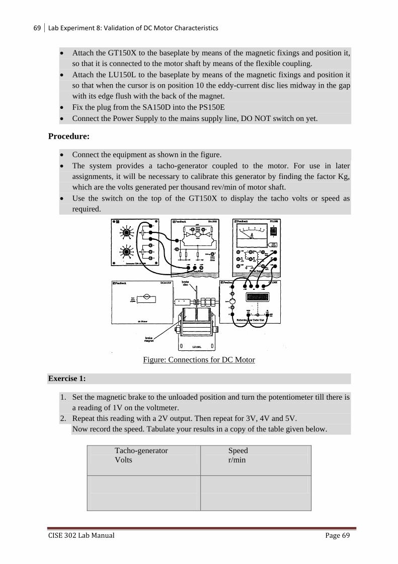
69 Lab Experiment 8: Validation of DC Motor Characteristics
CISE 302 Lab Manual Page 69
Attach the GT150X to the baseplate by means of the magnetic fixings and position it,
so that it is connected to the motor shaft by means of the flexible coupling.
Attach the LU150L to the baseplate by means of the magnetic fixings and position it
so that when the cursor is on position 10 the eddy-current disc lies midway in the gap
with its edge flush with the back of the magnet.
Fix the plug from the SA150D into the PS150E
Connect the Power Supply to the mains supply line, DO NOT switch on yet.
Procedure:
Connect the equipment as shown in the figure.
The system provides a tacho-generator coupled to the motor. For use in later
assignments, it will be necessary to calibrate this generator by finding the factor Kg,
which are the volts generated per thousand rev/min of motor shaft.
Use the switch on the top of the GT150X to display the tacho volts or speed as
required.
Figure: Connections for DC Motor
Exercise 1:
1. Set the magnetic brake to the unloaded position and turn the potentiometer till there is
a reading of 1V on the voltmeter.
2. Repeat this reading with a 2V output. Then repeat for 3V, 4V and 5V.
Now record the speed. Tabulate your results in a copy of the table given below.
Tacho-generator
Volts
Speed
r/min
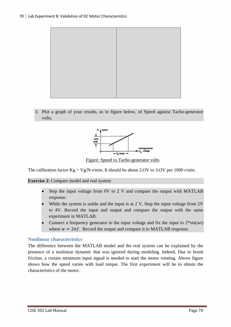
70 Lab Experiment 8: Validation of DC Motor Characteristics
CISE 302 Lab Manual Page 70
3. Plot a graph of your results, as in figure below, of Speed against Tacho-generator
volts.
Figure: Speed vs Tacho-generator volts
The calibration factor Kg = Vg/N-r/min. It should be about 2.OV to 3.OV per 1000 r/min.
Exercise 2: Compare model and real system
Step the input voltage from 0V to 2 V and compare the output with MATLAB
response.
While the system is stable and the input is at 2 V, Step the input voltage from 2V
to 4V. Record the input and output and compare the output with the same
experiment in MATLAB.
Connect a frequency generator to the input voltage and fix the input to 2*sin(wt)
where Record the output and compare it to MATLAB response.
Nonlinear characteristics
The difference between the MATLAB model and the real system can be explained by the
presence of a nonlinear dynamic that was ignored during modeling. Indeed, Due to brush
friction, a certain minimum input signal is needed to start the motor rotating. Above figure
shows how the speed varies with load torque. The first experiment will be to obtain the
characteristics of the motor.

71 Lab Experiment 8: Validation of DC Motor Characteristics
CISE 302 Lab Manual Page 71
Figure: Armature control characteristics
Exercise 3: determination of the nonlinear DC motor characteristics
Reduce the input voltage till the motor is just turning then measure with your voltmeter
the voltages between OV and potentiometer slider and the tacho-generator output.
Then tabulate as in fig 3.3.6. Increase the input voltage in one-volt steps, take readings
of the input voltage and tachogenerator voltage up to approximately 2000 r/min which
is the maximum speed of the motor.
Plot the input voltages against speed, your results should be similar to the figure which
shows plot of speed vs voltage.
Vin
Volts
Vg
Volts
Speed
rpm
Calculate the slope (input volts per thousand r/min).
Exercise 4: Effect of the load
To measure the torque/speed characteristics, fix the brake so that it passes over the
disc smoothly while the motor is running.
Set the brake at position 0 and increase the input voltage until the motor rotates at
close to its maximum speed.
Then set the brake at position 10 and if necessary reduce the input voltage so that the
ammeter on the PS150E is just below 2 amps; note the value of the input voltage.
72 Lab Experiment 8: Validation of DC Motor Characteristics
CISE 302 Lab Manual Page 72
Take tacho-generator readings over the range of the brake down to zero position,
tabulating your results.
Brake
Position
Vg
Volts
Speed
Rpm
Now reset the brake back to maximum position and reduce the signal input voltage so
that the motor is slowly rotating. Note the actual value of the input voltage.
Take readings over the brake range tabulating the further results.
Brake
Position
Vg
Volts
Speed
rpm
Plot the two sets of results, as in figure of Speed against Torque (brake position) for
the two input voltage values.
Below figure shows the approximate brake position/g.cm characteristics of the motor
at 1000 r/min. For other speeds, the torque will be proportional to the speed.
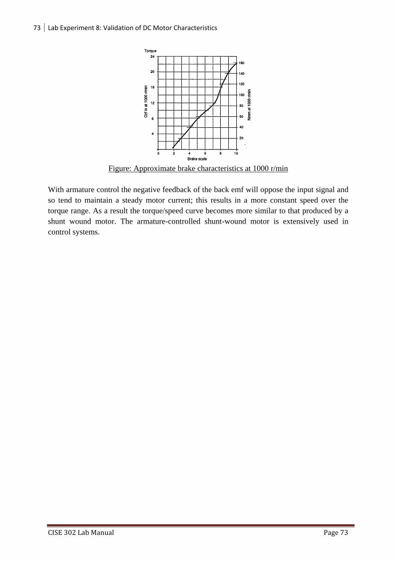
73 Lab Experiment 8: Validation of DC Motor Characteristics
CISE 302 Lab Manual Page 73
Figure: Approximate brake characteristics at 1000 r/min
With armature control the negative feedback of the back emf will oppose the input signal and
so tend to maintain a steady motor current; this results in a more constant speed over the
torque range. As a result the torque/speed curve becomes more similar to that produced by a
shunt wound motor. The armature-controlled shunt-wound motor is extensively used in
control systems.

74 Lab Experiment 9: Effect of Feedback on disturbance & Control System Design
CISE 302 Lab Manual Page 74
CISE 302
Linear Control Systems
Lab Experiment 9: Effect of Feedback on disturbance & Control System
Design
Objective: The objective of this exercise will be to study the effect of feedback on the
response of the system to step input and step disturbance taking the practical example of
English Channel boring machine and design a control system taking in account performance
measurement.
List of Equipment/Software
Following equipment/software is required:
MATLAB
Category Soft - Experiment
Deliverables
A complete lab report including the following:
Summarized learning outcomes.
The Simulink model.
MATLAB scripts and results for Exercise 1 & 2.
Overview: The construction of the tunnel under the English Channel from France to the Great Britain
began in December 1987. The first connection of the boring tunnels from each country was
achieved in November 1990. The tunnel is 23.5 miles long and bored 200 feet below sea
level. Costing $14 billion, it was completed in 1992 making it possible for a train to travel
from London to Paris in three hours.
The machine operated from both ends of the channel, bored towards the middle. To link up
accurately in the middle of the channel, a laser guidance system kept the machines precisely
aligned. A model of the boring machine control is shown in the figure, where Y(s) is the
actual angle of direction of travel of the boring machine and R(s) is the desired angle. The
effect of load on the machine is represented by the disturbance, Td(s).
Figure: A block diagram model of a boring machine control system
K s
Gc(s) Controller
s(s )
G(s) Plant
-
+ R(s)
Desired Angle
Y(s)
Angle +
+ Td(s)
75 Lab Experiment 9: Effect of Feedback on disturbance & Control System Design
CISE 302 Lab Manual Page 75
Exercise 1:
a) Get the transfer function from R(s) to Y(s)
b) Get the transfer function from D(s) to Y(s)
c) Generate the system response; for K= 10, 20, 50, 100; due to a unit step input - r(t)
d) Generate the system response; for K= 10, 20, 50, 100; due to a unit step disturbance -
d(t)
e) For each case find the percentage overshoot(%O.S.), rise time, settling time, steady
state of y(t)
f) Compare the results of the two cases
g) Investigate the effect of changing the controller gain on the influence of the
disturbance on the system output
M-files for two cases of K=20 and K=100 are shown below
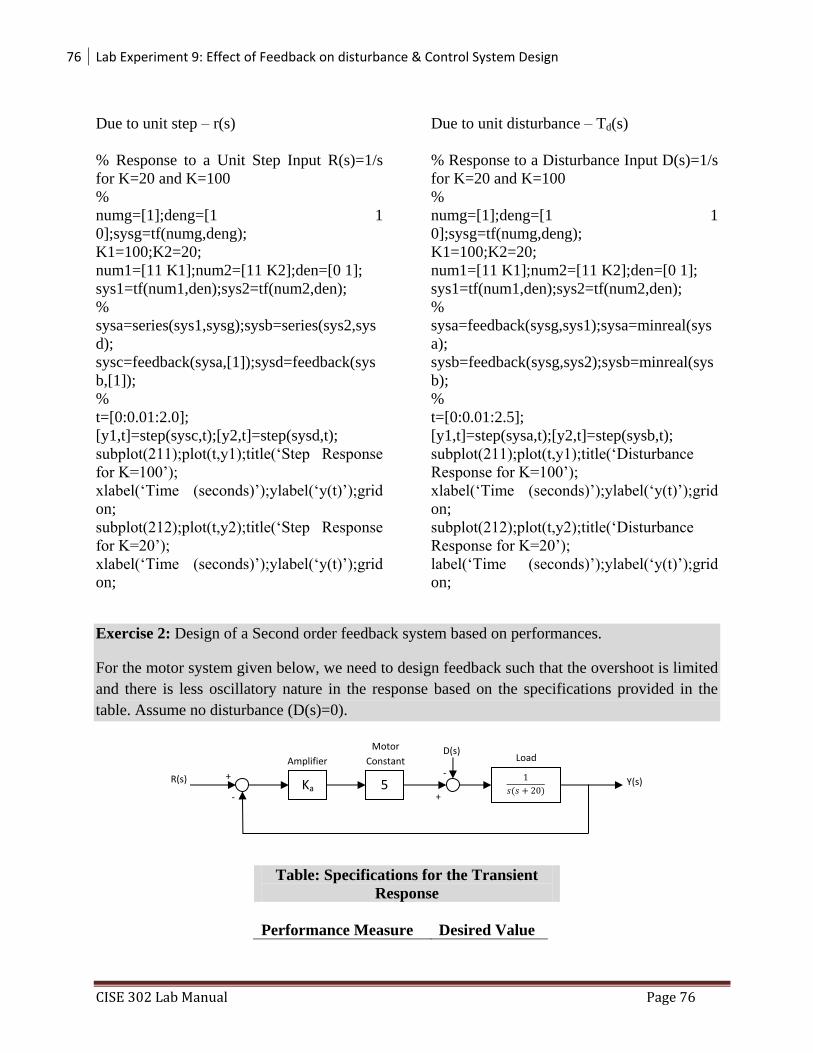
76 Lab Experiment 9: Effect of Feedback on disturbance & Control System Design
CISE 302 Lab Manual Page 76
Due to unit step – r(s)
% Response to a Unit Step Input R(s)=1/s
for K=20 and K=100
%
numg=[1];deng=[1 1
0];sysg=tf(numg,deng);
K1=100;K2=20;
num1=[11 K1];num2=[11 K2];den=[0 1];
sys1=tf(num1,den);sys2=tf(num2,den);
%
sysa=series(sys1,sysg);sysb=series(sys2,sys
d);
sysc=feedback(sysa,[1]);sysd=feedback(sys
b,[1]);
%
t=[0:0.01:2.0];
[y1,t]=step(sysc,t);[y2,t]=step(sysd,t);
subplot(211);plot(t,y1);title(‘Step Response
for K=100’);
xlabel(‘Time (seconds)’);ylabel(‘y(t)’);grid
on;
subplot(212);plot(t,y2);title(‘Step Response
for K=20’);
xlabel(‘Time (seconds)’);ylabel(‘y(t)’);grid
on;
Due to unit disturbance – Td(s)
% Response to a Disturbance Input D(s)=1/s
for K=20 and K=100
%
numg=[1];deng=[1 1
0];sysg=tf(numg,deng);
K1=100;K2=20;
num1=[11 K1];num2=[11 K2];den=[0 1];
sys1=tf(num1,den);sys2=tf(num2,den);
%
sysa=feedback(sysg,sys1);sysa=minreal(sys
a);
sysb=feedback(sysg,sys2);sysb=minreal(sys
b);
%
t=[0:0.01:2.5];
[y1,t]=step(sysa,t);[y2,t]=step(sysb,t);
subplot(211);plot(t,y1);title(‘Disturbance
Response for K=100’);
xlabel(‘Time (seconds)’);ylabel(‘y(t)’);grid
on;
subplot(212);plot(t,y2);title(‘Disturbance
Response for K=20’);
label(‘Time (seconds)’);ylabel(‘y(t)’);grid
on;
Exercise 2: Design of a Second order feedback system based on performances.
For the motor system given below, we need to design feedback such that the overshoot is limited
and there is less oscillatory nature in the response based on the specifications provided in the
table. Assume no disturbance (D(s)=0).
Table: Specifications for the Transient
Response
Performance Measure
Desired Value
Ka 5
𝑠(𝑠 )
R(s)
-
+
+
- Y(s)
Amplifier
Motor
Constant Load D(s)
Create subplots with x
and y axis labels
Closed loop transfer
functions
Choose time interval
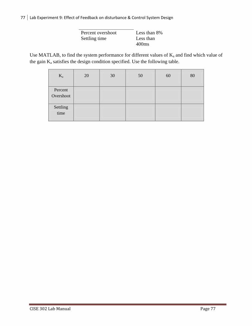
77 Lab Experiment 9: Effect of Feedback on disturbance & Control System Design
CISE 302 Lab Manual Page 77
Percent overshoot Less than 8%
Settling time Less than
400ms
Use MATLAB, to find the system performance for different values of Ka and find which value of
the gain Ka satisfies the design condition specified. Use the following table.
Ka 20 30 50 60 80
Percent
Overshoot
Settling
time

78 Lab Experiment 10: Effect of Feedback on disturbance & Control System Design of Tank Level System
CISE 302 Lab Manual Page 78
CISE 302
Linear Control Systems
Lab Experiment 10: Effect of Feedback on disturbance & Control System
Design of Tank Level System
Objective: The objective of this exercise will be to study the effect of feedback on the
response of the system to step input and step disturbance on the Two Tank System.
List of Equipment/Software
Following equipment/software is required:
MATLAB
LabVIEW
NI USB 6009 Data Acquisition Card
Two Tank System (CE 105)
Category Software Hardware Experiment
Deliverables
A complete lab report including the following:
Summarized learning outcomes.
LabVIEW programming files (Block diagram and Front Panel)
Graphical representation of data collected for several cases of disturbance (leakage via
valve at bottom). (Instructors should provide the data collection VI file)
Controller performance and parameters for each case of disturbance.
Overview:
A model of the tank system and the controller is shown in the figure, where Y(s) is the actual
level of the tank and R(s) is the desired level. The effect of disturbance to the tank system is
represented by the disturbance, Td(s). The Td(s) is the leakage that can be generated from the
hand valve at the bottom of the tank system.

79 Lab Experiment 10: Effect of Feedback on disturbance & Control System Design of Tank Level System
CISE 302 Lab Manual Page 79
Figure: A block diagram model of a two tank level control system
NOTE: Instructors should manage to complete the hardware/software setup for the students to
take reading and implement the controller.
Exercise:
a) Launch the data collection LabVIEW file and make the proper connections to the Two
Tank System. This experiment uses only one tank of the system.
b) The disturbance to the tank is the hand-valve in the bottom of the first tank.
c) Collect the data for the FIVE cases of leakage valve (valve at bottom).
d) From the theory and understanding from last experiment (Exp 7), identify and prepare the
transfer function and respective controllers for the specifications discussed during last
experiment.
e) Generate the system response; for K= 10, 20, 50, 100; due to the five cases of leakage
disturbance - d(t)
f) For each case find the percentage overshoot(%O.S.), rise time, settling time, steady state
of y(t)
g) Compare the results of all the cases
h) Investigate the effect of changing the controller gain on the influence of the disturbance
on the system output
Gc(s) Controller
G(s) Plant
-
+ R(s)
Desired Level
Y(s)
Height
(Level of
tank)
+
+ Leakage Td(s)

80 Lab Experiment 11: Introduction to PID controller
CISE 302 Lab Manual Page 80
CISE 302
Linear Control Systems
Lab Experiment 11: Introduction to PID controller
Objective: Study the three term (PID) controller and its effects on the feedback loop response.
Investigate the characteristics of the each of proportional (P), the integral (I), and the derivative
(D) controls, and how to use them to obtain a desired response.
List of Equipment/Software
Following equipment/software is required:
MATLAB
LabVIEW
Category Soft - Experiment
Deliverables
A complete lab report including the following:
Summarized learning outcomes.
LabVIEW programming files (Block diagram and Front Panel)
Controller design and parameters for each of the given exercises.
Introduction: Consider the following unity feedback system:
Plant: A system to be controlled.
Controller: Provides excitation for the plant; Designed to control the overall system behavior.
The three-term controller: The transfer function of the PID controller looks like the following:
Controller Plant R e u Y +
-

81 Lab Experiment 11: Introduction to PID controller
CISE 302 Lab Manual Page 81
KP = Proportional gain
KI = Integral gain
KD = Derivative gain
First, let's take a look at how the PID controller works in a closed-loop system using the
schematic shown above. The variable (e) represents the tracking error, the difference between the
desired input value (R) and the actual output (Y). This error signal (e) will be sent to the PID
controller, and the controller computes both the derivative and the integral of this error signal.
The signal (u) just past the controller is now equal to the proportional gain (KP) times the
magnitude of the error plus the integral gain (KI) times the integral of the error plus the
derivative gain (KD) times the derivative of the error.
( ) ∫ ( ) ( )
This signal (u) will be sent to the plant, and the new output (Y) will be obtained. This new output
(Y) will be sent back to the sensor again to find the new error signal (e). The controller takes this
new error signal and computes its derivatives and its internal again. The process goes on and on.
Example Problem:
Suppose we have a simple mass, spring, and damper problem.
The modeling equation of this system is
Taking the Laplace transform of the modeling equation (1), we get
( ) ( ) ( ) ( )
The transfer function between the displacement X(s) and the input F(s) then becomes

82 Lab Experiment 11: Introduction to PID controller
CISE 302 Lab Manual Page 82
( )
( )
Let
M = 1kg
b = 10 N.s/m
k = 20 N/m
F(s) = 1
Plug these values into the above transfer function
( )
( )
The goal of this problem is to show you how each of Kp, Ki and Kd contributes to obtain
Fast rise time
Minimum overshoot
No steady-state error
Open-loop step response: Let's first view the open-loop step response.
num=1;
den=[1 10 20];
plant=tf(num,den);
step(plant)
MATLAB command window should give you the plot shown below.
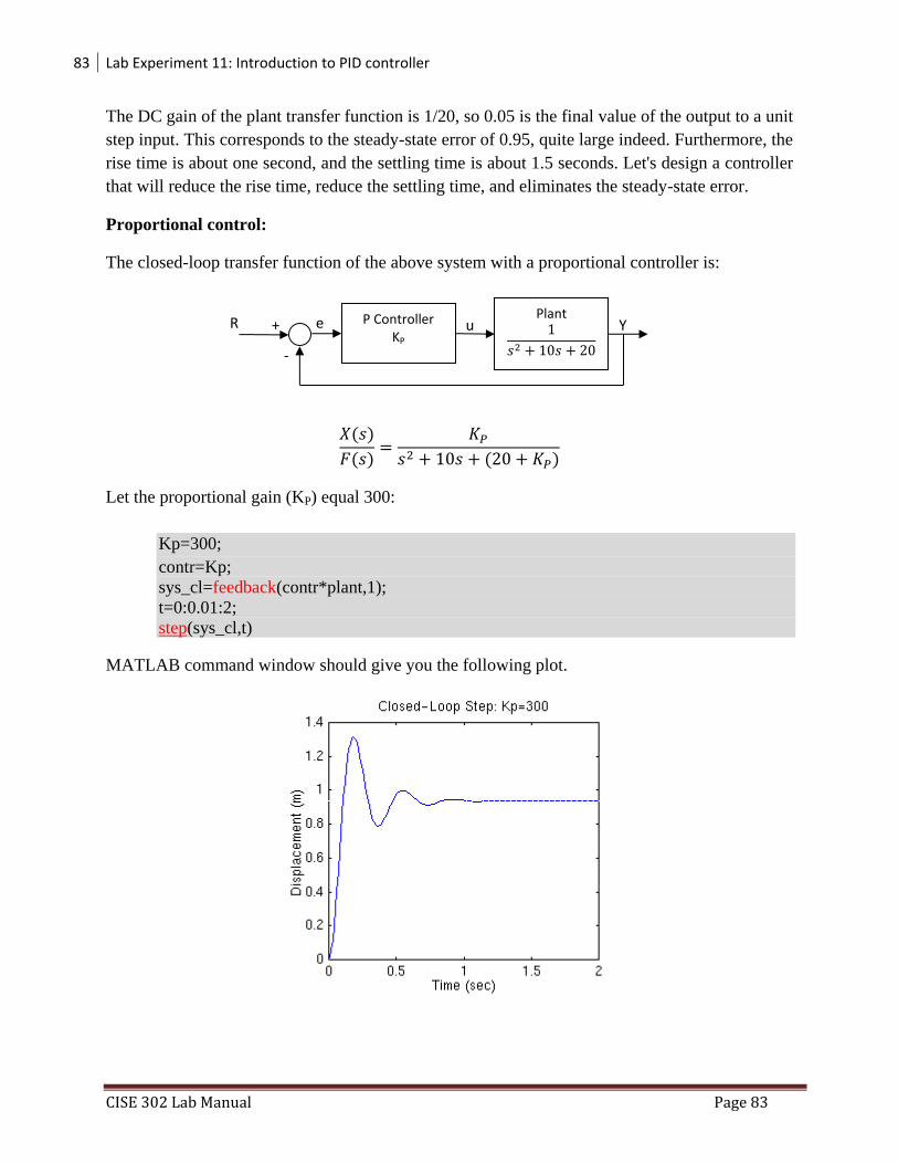
83 Lab Experiment 11: Introduction to PID controller
CISE 302 Lab Manual Page 83
The DC gain of the plant transfer function is 1/20, so 0.05 is the final value of the output to a unit
step input. This corresponds to the steady-state error of 0.95, quite large indeed. Furthermore, the
rise time is about one second, and the settling time is about 1.5 seconds. Let's design a controller
that will reduce the rise time, reduce the settling time, and eliminates the steady-state error.
Proportional control:
The closed-loop transfer function of the above system with a proportional controller is:
( )
( )
( )
Let the proportional gain (KP) equal 300:
Kp=300;
contr=Kp;
sys_cl=feedback(contr*plant,1);
t=0:0.01:2;
step(sys_cl,t)
MATLAB command window should give you the following plot.
P Controller KP
𝑠 𝑠
Plant R e u Y +
-
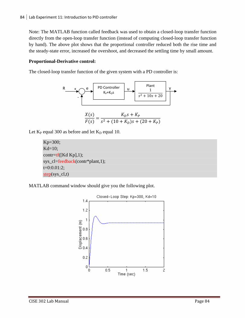
84 Lab Experiment 11: Introduction to PID controller
CISE 302 Lab Manual Page 84
Note: The MATLAB function called feedback was used to obtain a closed-loop transfer function
directly from the open-loop transfer function (instead of computing closed-loop transfer function
by hand). The above plot shows that the proportional controller reduced both the rise time and
the steady-state error, increased the overshoot, and decreased the settling time by small amount.
Proportional-Derivative control:
The closed-loop transfer function of the given system with a PD controller is:
( )
( )
( ) ( )
Let KP equal 300 as before and let KD equal 10.
Kp=300;
Kd=10;
contr=tf([Kd Kp],1);
sys_cl=feedback(contr*plant,1);
t=0:0.01:2;
step(sys_cl,t)
MATLAB command window should give you the following plot.
PD Controller KP+KDs
𝑠 𝑠
Plant R e u Y +
-
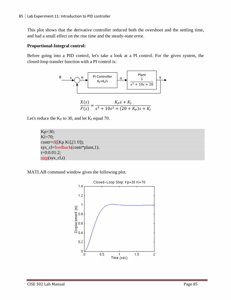
85 Lab Experiment 11: Introduction to PID controller
CISE 302 Lab Manual Page 85
This plot shows that the derivative controller reduced both the overshoot and the settling time,
and had a small effect on the rise time and the steady-state error.
Proportional-Integral control:
Before going into a PID control, let's take a look at a PI control. For the given system, the
closed-loop transfer function with a PI control is:
( )
( )
( )
Let's reduce the KP to 30, and let KI equal 70.
Kp=30;
Ki=70;
contr=tf([Kp Ki],[1 0]);
sys_cl=feedback(contr*plant,1);
t=0:0.01:2;
step(sys_cl,t)
MATLAB command window gives the following plot.
PI Controller KP+KI/s
𝑠 𝑠
Plant R e u Y +
-

86 Lab Experiment 11: Introduction to PID controller
CISE 302 Lab Manual Page 86
We have reduced the proportional gain (Kp) because the integral controller also reduces the rise
time and increases the overshoot as the proportional controller does (double effect). The above
response shows that the integral controller eliminated the steady-state error.
Proportional-Integral-Derivative control:
Now, let's take a look at a PID controller. The closed-loop transfer function of the given system
with a PID controller is:
( )
( )
( ) ( )
After several trial and error runs, the gains Kp=350, Ki=300, and Kd=50 provided the desired
response. To confirm, enter the following commands to an m-file and run it in the command
window. You should get the following step response.
Kp=350;
Ki=300;
Kd=50;
contr=tf([Kd Kp Ki],[1 0]);
sys_cl=feedback(contr*plant,1);
t=0:0.01:2;
step(sys_cl,t)
PID Controller KP+KI/s+ KDs
𝑠 𝑠
Plant R e u Y +
-

87 Lab Experiment 11: Introduction to PID controller
CISE 302 Lab Manual Page 87
Now, we have obtained a closed-loop system with no overshoot, fast rise time, and no steady-
state error.
The characteristics of P, I, and D controllers:
The proportional controller (KP) will have the effect of reducing the rise time and will reduce,
but never eliminate, the steady state error. An integral controller (KI) will have the effect of
eliminating the steady state error, but it may make the transient response worse. A derivative
control (KD) will have the effect of increasing the stability of the system, reducing the overshoot
and improving the transient response.
Effect of each controller KP, KI and KD on the closed-loop system are summarized below
CL Response Rise Time Overshoot Settling Time S-S Error
KP Decrease Increase Small Change Decrease
KI Decrease Increase Increases Eliminate
KD Small Change Decreases Decreases Small Change
Note that these corrections may not be accurate, because KP, KI, and KD are dependent of each
other. In fact, changing one of these variables can change the effect of the other two. For this
reason the table should only be used as a reference when you are determining the values for KP,
KI, and KD.
Exersice:
Consider a process given below to be controlled by a PID controller,
)5.48(
400)(
sssGp
a) Obtain the unit step response of Gp(s).
b) Try PI controllers with (Kp=2, 10, 100), and Ki=Kp/10. Investigate the unit step
response in each case, compare the results and comment.
c) Let Kp=100, Ki=10, and add a derivative term with (Kd=0.1, 0.9, 2). Investigate the unit
step response in each case, compare the results and comment.
Based on your results in parts b) and c) above what do you conclude as a suitable PID controller
for this process and give your justification.

88 Lab Experiment 12: Open Loop and Closed Loop position control of DC Motor
CISE 302 Lab Manual Page 88
CISE 302
Linear Control Systems
Lab Experiment 12: Open Loop and Closed Loop position control of DC
Motor
Objective: To familiarize the servo motor system and experience the open and closed loop
control of servo system to be used in an automatic position control system.
List of Equipment/Software
Following equipment/software is required:
LabVIEW
DC Servo System (feedback equipment)
a. OU150A Op Amp Unit
b. AU150B Attenuator Unit
c. PA150C Pre-Amplifier Unit
d. SA150D Servo Amplifier
e. PS150E Power Supply
f. DCM150F DC Motor
g. IP150H Input Potentiometer
h. OP150K Output Potentiometer
i. GT150X Reduction Gear Tacho
j. DC Voltmeter
Category Software-Hardware Experiment
Deliverables
A complete lab report including the following:
Summarized learning outcomes.
Connection diagram of the hardware experimental part.
Report the procedure and troubleshooting during the experiment.
Show results for the open loop and closed loop position control via graphs and tables.
Report the LabVIEW program components i.e., Front Panel and Block Diagram.
Procedure (Open loop position control):

89 Lab Experiment 12: Open Loop and Closed Loop position control of DC Motor
CISE 302 Lab Manual Page 89
1. Attach the AU150B, SA150D and DCM150F to the baseplate by means of the magnetic
fixings.
2. Fix the plugs from the servo amplifier into the power supply.
3. Fix the plug from the motor unit into the servo amplifier.
4. Attach the GT150X to the baseplate by means of the magnetic fixing and position it so
that it is connected to the motor shaft by means of the flexible coupling.
5. Set up for open loop as shown in Fig. 1.
6. Use a push-on coupling to link a low-speed shaft of the GT150X to the output
potentiometer shaft.
7. Starting with AU150B the potentiometer knob at the fully counter-clockwise position
gradually turn it till the motor just rotates and record:
8. Scale position at which the motor just rotates: ..........................(1)
9. Direction in which the output rotary potentiometer moves: ........................ (2)
10. Return the output rotary potentiometer cursor to zero by turning the GT150X high-speed
shaft.
11. Decide on a position in the direction (2), you wish the potentiometer shaft to turn to and
then turn the AU150B potentiometer knob to position (1). As the cursor nears the
required angle, reduce this input signal so that the cursor comes to rest nearly at the
required point.
The open loop system will have you as a feedback. Such a system could be shown as in the
figure.

90 Lab Experiment 12: Open Loop and Closed Loop position control of DC Motor
CISE 302 Lab Manual Page 90
Figure 1: Open loop System (with you as feedback)

91 Lab Experiment 12: Open Loop and Closed Loop position control of DC Motor
CISE 302 Lab Manual Page 91
Procedure (Closed loop position control):
1. Set the apparatus as shown in Fig.2 for closed loop control.
2. This shall utilize the error signal output VO of the operational amplifier to drive the
output potentiometer via the pre-amplifier and motor.
3. The upper potentiometer on the AU150B can now be used as a gain control and should
initially be set to zero before switching on the power.
4. Adjust the PA150C `zero set' so that the motor does not rotate.
5. Now set the IP150H to some arbitrary angle and increase the gain control setting.
6. The output potentiometer cursor should rotate to an angle nearly equal to that of the input
potentiometer cursor.
Trouble-shooting:
Output potentiometer (or the motor) is oscillating:
Make sure that the upper potentiometer on the AU150B is all down to zero (i.e.
the gain is equal to zero) and then rotate the zero set knob on pre-amplifier
PA150C so that the motor stop rotating or oscillating.
After increasing the gain (i.e. make the upper potentiometer on the AU150B other
than zero) the motor behaves in the same way then change the order of connection
from pre-amplifier to servo-amplifier (i.e. if the output “3” and “4” of pre-
amplifier PA150C is connected to input “1” and “2” of the servo-amplifier
SA150D respectively then change it such that the output “3” and “4” of pre-
amplifier PA150C is connected to input “2” and “1” of the servo-amplifier
SA150D respectively or vice-versa)
Output potentiometer is not following input potentiometer: in such cases there
is misalignment. Please hold the outer disc of input potentiometer IP150H firmly
and rotate its knob making sure that the disc does not rotate. Doing this make sure
that the input potentiometer “0” angle matches with the output potentiometer “0”
angle.
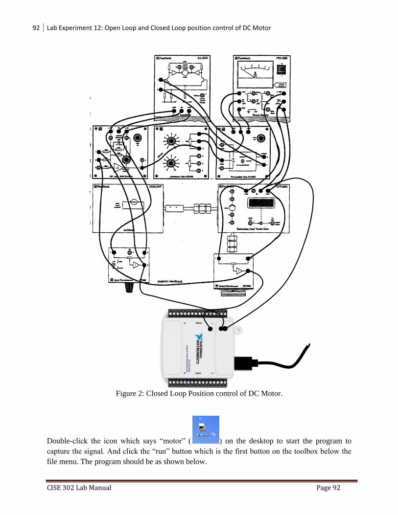
92 Lab Experiment 12: Open Loop and Closed Loop position control of DC Motor
CISE 302 Lab Manual Page 92
Figure 2: Closed Loop Position control of DC Motor.
Double-click the icon which says “motor” ( ) on the desktop to start the program to
capture the signal. And click the “run” button which is the first button on the toolbox below the
file menu. The program should be as shown below.

93 Lab Experiment 12: Open Loop and Closed Loop position control of DC Motor
CISE 302 Lab Manual Page 93
Identify from the setup the equipment which should be place in the following block diagram
Plant equipment
SA150D,__________,_________________,__________,OP150K
__
IP150H Y(s) +
-
Controller equipment
_________
PA150C
94 Lab Experiment 13: Simple Speed Control of DC Motor
CISE 302 Lab Manual Page 94
CISE 302
Linear Control Systems
Lab Experiment 13: Simple Speed Control of DC Motor
Objective: Observe how the Simple Speed control system is constructed and appreciate the
importance of Tacho-generator in closed-loop speed control system.
List of Equipment/Software
Following equipment/software is required:
LabVIEW
DC Servo System (feedback equipment)
a. OU150A Op Amp Unit
b. AU150B Attenuator Unit
c. PA150C Pre-Amplifier Unit
d. SA150D Servo Amplifier
e. PS150E Power Supply
f. DCM150F DC Motor
g. IP150H Input Potentiometer
h. OP150K Output Potentiometer
i. GT150X Reduction Gear Tacho
j. DC Voltmeter
Category Software-Hardware Experiment
Deliverables
A complete lab report including the following:
Summarized learning outcomes.
Connection diagram of the hardware experimental part.
Report the procedure and troubleshooting during the experiment.
Show results for the open loop and closed loop speed control via graphs and tables.
Introduction: In the last experiments we saw how simple position control could be constructed. In today's
assignment we shall see how simple speed control of motor could be done. In the experiment
involving the DC Motor Characteristics we saw how the signal inputs into SA150D could vary
the speed of the motor. This means that without any load you can set the motor to run at
specified speed determining the value of the input signal. What kind of speed control was it?

95 Lab Experiment 13: Simple Speed Control of DC Motor
CISE 302 Lab Manual Page 95
Now if we look at the torque/speed characteristics in the experiment, we can say that if load is
placed on the motor the speed of the motor will change to some extent. With open-loop system
the results show that there can be a reasonable speed control when operating without or with a
fixed load but the system would be very unsuitable where the load was varying.
With closed load, we will show improvement in speed control with respect to varying load. That
is, the actual speed will be compared to the required speed. This produces an error signal to
actuate the servo amplifier output so that the motor maintains a more constant speed.
Exercise 1: Simple feedback speed-control without load.
In this exercise we will simply feedback a signal proportional to the speed, using the Tacho-
generator. We then compare it with a reference signal of opposite polarity, so that the sum will
produce an input signal into the servo amplifier of the required value. As comparator, we will use
an operational amplifier.
On the OA150A set the 'feedback selector' to 100KΩ resistor

96 Lab Experiment 13: Simple Speed Control of DC Motor
CISE 302 Lab Manual Page 96
Before connecting the Tacho-generator to an input of the OA150A, increase the 'reference'
voltage so that the motor revolves and on your voltmeter determine which the Tacho’s positive
output is. The correct side can then be connected to OA150A input and the other side to 0V.
Reset the reference voltage to zero and then gradually increase it so that you can take readings
over the motor speed range of upto approximately 2000 r/min for the reference, tacho-generator
and error voltages.
Record your results in the following table
Plot the error voltage against speed.
Speed Reference
Voltage
Tacho-generator
voltage
Error
Voltage
200
400
600
800
1000
1200
1400
1600
1800
2000

97 Lab Experiment 13: Simple Speed Control of DC Motor
CISE 302 Lab Manual Page 97
Exercise 2: Effect of Load on Speed
To find the effect of the load on speed we can user the magnetic brake as a load. The change in
speed for a change in load will give us the regulation. Ensure that the eddy current brake disc is
fitted to the motor. Also ensure that the load unit can be fully engaged without fouling either the
motor mount or the eddy current disc.
The exercise is concerned to show how an increase in the forward path gain will cause a given
fall in speed to cause a larger increase in the value of the error V0, so that for any change in load
the speed drop or 'droop' will decrease with increase gain as shown in the figure.
For a gain control we can use the circuit given above, which has a gain of -1/α.

98 Lab Experiment 13: Simple Speed Control of DC Motor
CISE 302 Lab Manual Page 98
On the OA150A set the 'feedback selector' switch to 'external feedback'. On the LU150L swing
the magnets clear. Initially set the gain to unity, that is to position 10 of the upper potentiometer
and adjust the reference volts till the motor runs at 1000 r/min. Then take readings of the
reference voltage, Vin, Error voltage, Ve and the Tacho-generator voltage, using the voltmeter,
over the range of brake positions 0 – 10 and then tabulate your results in the following table. Be
careful that you do not exceed the 2A limiting current. Repeat the readings for a gain of 5,
which is to set the gain potentiometer to position 1. Re-adjust the reference potentiometer to give
no-load motor speed of 1000 r/min.

99 Lab Experiment 13: Simple Speed Control of DC Motor
CISE 302 Lab Manual Page 99
For gain of 1 For gain of 5
Brake
Position
Reference
(Vin)
volts
Tacho-
generator
volts
Error
(Ve)
volts
Speed
r/min
1
2
3
4
5
6
7
8
9
10
Brake
Position
Reference
(Vin)
volts
Tacho-
generator
volts
Error
(Ve)
volts
Speed
r/min
1
2
3
4
5
6
7
8
9
10
Plot your results in the form of graphs of error voltage against brake setting and speed for
gain values of 1 and 5.
Exercise 3: Reversible speed control
In the last part of the experiment we will assemble a simple reversible speed control system.
From your reading you have seen that a high gain decreases the minimum reference signal
needed for the motor to respond so this exercise we will use high gain.
The inputs into the SA150D can drive the motor in opposite directions but both inputs require
positive voltages. As the output of the OA 150A varies from positive to negative it is
necessary to use the PA150C pre-amplifier unit that is so designed that a negative input gives
a positive voltage on output and a negative input gives a positive voltage on the other output
with a gain of about 25.
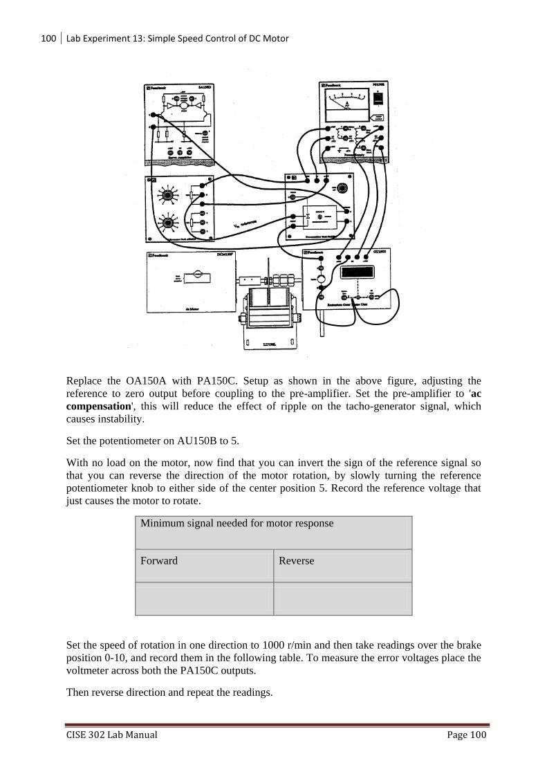
100 Lab Experiment 13: Simple Speed Control of DC Motor
CISE 302 Lab Manual Page 100
Replace the OA150A with PA150C. Setup as shown in the above figure, adjusting the
reference to zero output before coupling to the pre-amplifier. Set the pre-amplifier to 'ac
compensation', this will reduce the effect of ripple on the tacho-generator signal, which
causes instability.
Set the potentiometer on AU150B to 5.
With no load on the motor, now find that you can invert the sign of the reference signal so
that you can reverse the direction of the motor rotation, by slowly turning the reference
potentiometer knob to either side of the center position 5. Record the reference voltage that
just causes the motor to rotate.
Minimum signal needed for motor response
Forward Reverse
Set the speed of rotation in one direction to 1000 r/min and then take readings over the brake
position 0-10, and record them in the following table. To measure the error voltages place the
voltmeter across both the PA150C outputs.
Then reverse direction and repeat the readings.
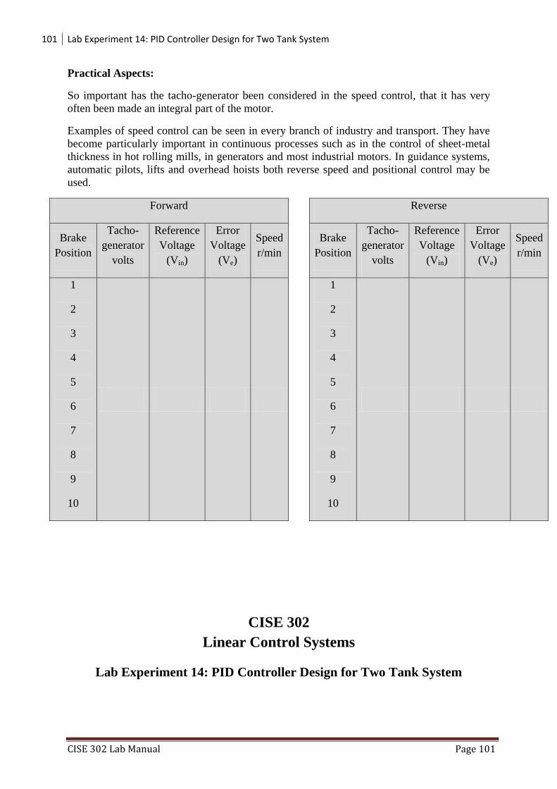
101 Lab Experiment 14: PID Controller Design for Two Tank System
CISE 302 Lab Manual Page 101
Practical Aspects:
So important has the tacho-generator been considered in the speed control, that it has very
often been made an integral part of the motor.
Examples of speed control can be seen in every branch of industry and transport. They have
become particularly important in continuous processes such as in the control of sheet-metal
thickness in hot rolling mills, in generators and most industrial motors. In guidance systems,
automatic pilots, lifts and overhead hoists both reverse speed and positional control may be
used.
Forward
Brake
Position
Tacho-
generator
volts
Reference
Voltage
(Vin)
Error
Voltage
(Ve)
Speed
r/min
1
2
3
4
5
6
7
8
9
10
Reverse
Brake
Position
Tacho-
generator
volts
Reference
Voltage
(Vin)
Error
Voltage
(Ve)
Speed
r/min
1
2
3
4
5
6
7
8
9
10
CISE 302
Linear Control Systems
Lab Experiment 14: PID Controller Design for Two Tank System

102 Lab Experiment 14: PID Controller Design for Two Tank System
CISE 302 Lab Manual Page 102
Objective: To familiarize the Two Tank System and experience the PID controller design
to control the level of the tank system.
List of Equipment/Software
Following equipment/software is required:
LabVIEW
NI USB 6009 Data Acquisition Card
Two Tank System
Category Software-Hardware Experiment
Deliverables
A complete lab report including the following:
Summarized learning outcomes.
Show the PID block diagram and the controller parameters with the process graphs.
Report the LabVIEW program components i.e., Front Panel and Block Diagram.
The USB DAQ
Interfacing the Two tank
In this exercise, two-tank system is introduced. The two tank system is as shown in the
figure. It has a water pump which takes in 0..10 voltages and pumps in water with speeds
depending at the voltage supplied. Two outputs which are the speed of flow and the level of
water in the tank are shown visually. There are speed and level sensors that provide voltages
between 0 and 10 voltages to indicate speed and voltage. The yellow filled area shows the
flow of water from pump to tank to reservoir through valves. The flow from tank to reservoir
can be controlled using the value. At “0” indicator the valve is “fully closed” and at “5” it is
“fully opened”.
The Two Tank System
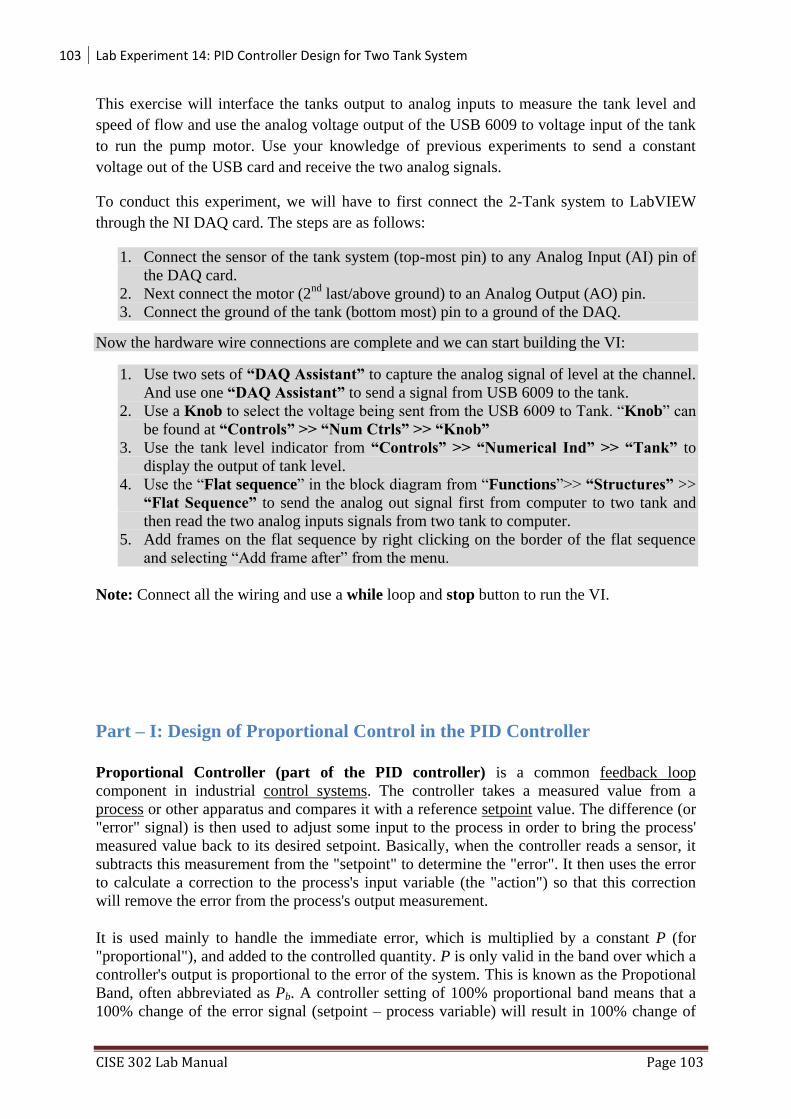
103 Lab Experiment 14: PID Controller Design for Two Tank System
CISE 302 Lab Manual Page 103
This exercise will interface the tanks output to analog inputs to measure the tank level and
speed of flow and use the analog voltage output of the USB 6009 to voltage input of the tank
to run the pump motor. Use your knowledge of previous experiments to send a constant
voltage out of the USB card and receive the two analog signals.
To conduct this experiment, we will have to first connect the 2-Tank system to LabVIEW
through the NI DAQ card. The steps are as follows:
1. Connect the sensor of the tank system (top-most pin) to any Analog Input (AI) pin of
the DAQ card.
2. Next connect the motor (2nd
last/above ground) to an Analog Output (AO) pin.
3. Connect the ground of the tank (bottom most) pin to a ground of the DAQ.
Now the hardware wire connections are complete and we can start building the VI:
1. Use two sets of “DAQ Assistant” to capture the analog signal of level at the channel.
And use one “DAQ Assistant” to send a signal from USB 6009 to the tank.
2. Use a Knob to select the voltage being sent from the USB 6009 to Tank. “Knob” can
be found at “Controls” >> “Num Ctrls” >> “Knob”
3. Use the tank level indicator from “Controls” >> “Numerical Ind” >> “Tank” to
display the output of tank level.
4. Use the “Flat sequence” in the block diagram from “Functions”>> “Structures” >>
“Flat Sequence” to send the analog out signal first from computer to two tank and
then read the two analog inputs signals from two tank to computer.
5. Add frames on the flat sequence by right clicking on the border of the flat sequence
and selecting “Add frame after” from the menu.
Note: Connect all the wiring and use a while loop and stop button to run the VI.
Part – I: Design of Proportional Control in the PID Controller
Proportional Controller (part of the PID controller) is a common feedback loop
component in industrial control systems. The controller takes a measured value from a
process or other apparatus and compares it with a reference setpoint value. The difference (or
"error" signal) is then used to adjust some input to the process in order to bring the process'
measured value back to its desired setpoint. Basically, when the controller reads a sensor, it
subtracts this measurement from the "setpoint" to determine the "error". It then uses the error
to calculate a correction to the process's input variable (the "action") so that this correction
will remove the error from the process's output measurement.
It is used mainly to handle the immediate error, which is multiplied by a constant P (for
"proportional"), and added to the controlled quantity. P is only valid in the band over which a
controller's output is proportional to the error of the system. This is known as the Propotional
Band, often abbreviated as Pb. A controller setting of 100% proportional band means that a
100% change of the error signal (setpoint – process variable) will result in 100% change of
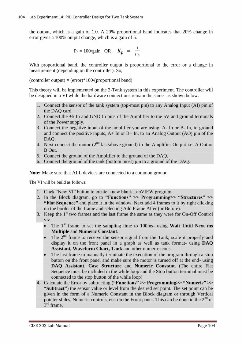
104 Lab Experiment 14: PID Controller Design for Two Tank System
CISE 302 Lab Manual Page 104
the output, which is a gain of 1.0. A 20% proportional band indicates that 20% change in
error gives a 100% output change, which is a gain of 5.
Pb = 100/gain OR
With proportional band, the controller output is proportional to the error or a change in
measurement (depending on the controller). So,
(controller output) = (error)*100/(proportional band)
This theory will be implemented on the 2-Tank system in this experiment. The controller will
be designed in a VI while the hardware connections remain the same- as shown below:
1. Connect the sensor of the tank system (top-most pin) to any Analog Input (AI) pin of
the DAQ card.
2. Connect the +5 In and GND In pins of the Amplifier to the 5V and ground terminals
of the Power supply.
3. Connect the negative input of the amplifier you are using, A- In or B- In, to ground
and connect the positive inputs, A+ In or B+ In, to an Analog Output (AO) pin of the
DAQ.
4. Next connect the motor (2nd
last/above ground) to the Amplifier Output i.e. A Out or
B Out.
5. Connect the ground of the Amplifier to the ground of the DAQ.
6. Connect the ground of the tank (bottom most) pin to a ground of the DAQ.
Note: Make sure that ALL devices are connected to a common ground.
The VI will be build as follows:
1. Click “New VI” button to create a new blank LabVIEW program.
2. In the Block diagram, go to “Functions” >> Programming>> “Structures” >>
“Flat Sequence” and place it in the window. Next add 4 frames to it by right clicking
on the border of the frame and selecting Add Frame After (or Before).
3. Keep the 1st two frames and the last frame the same as they were for On-Off Control
viz.
The 1st frame to set the sampling time to 100ms- using Wait Until Next ms
Multiple and Numeric Constant.
The 2nd
frame to receive the sensor signal from the Tank, scale it properly and
display it on the front panel in a graph as well as tank format- using DAQ
Assistant, Waveform Chart, Tank and other numeric icons.
The last frame to manually terminate the execution of the program through a stop
button on the front panel and make sure the motor is turned off at the end- using
DAQ Assistant, Case Structure and Numeric Constant. (The entire Flat
Sequence must be included in the while loop and the Stop button terminal must be
connected to the stop button of the while loop)
4. Calculate the Error by subtracting (“Functions” >> Programming>> “Numeric” >>
“Subtract”) the sensor value or level from the desired set point. The set point can be
given in the form of a Numeric Constant in the Block diagram or through Vertical
pointer slides, Numeric controls, etc. on the Front panel. This can be done in the 2nd
or
3rd
frame.

105 Lab Experiment 14: PID Controller Design for Two Tank System
CISE 302 Lab Manual Page 105
5. On the front panel, add a Control Knob from the Numeric palette. This will be used to
control the Proportional gain Kp. In the 3rd
frame of the Block diagram sequence,
multiply the error with the gain- connect the error and gain terminal to a
multiplication block.
6. In the same frame check the above product (input to controller) and if it is greater than
1 send one to the Tank system- using DAQ. If it is lesser than 0 send the tank 0. If it is
between 0 and 1, send the control input as it is. The comparison can be done using
“Greater Or Equal?” and “Lesser Or Equal?” functions along with a Case Structure
having another Case Structure inside (as in the On-Off Control). Here the control
input is connected to the Case Selector.
7. After all the wiring is complete switch to Front Panel and press the RUN button to
execute the VI.

106 Lab Experiment 14: PID Controller Design for Two Tank System
CISE 302 Lab Manual Page 106
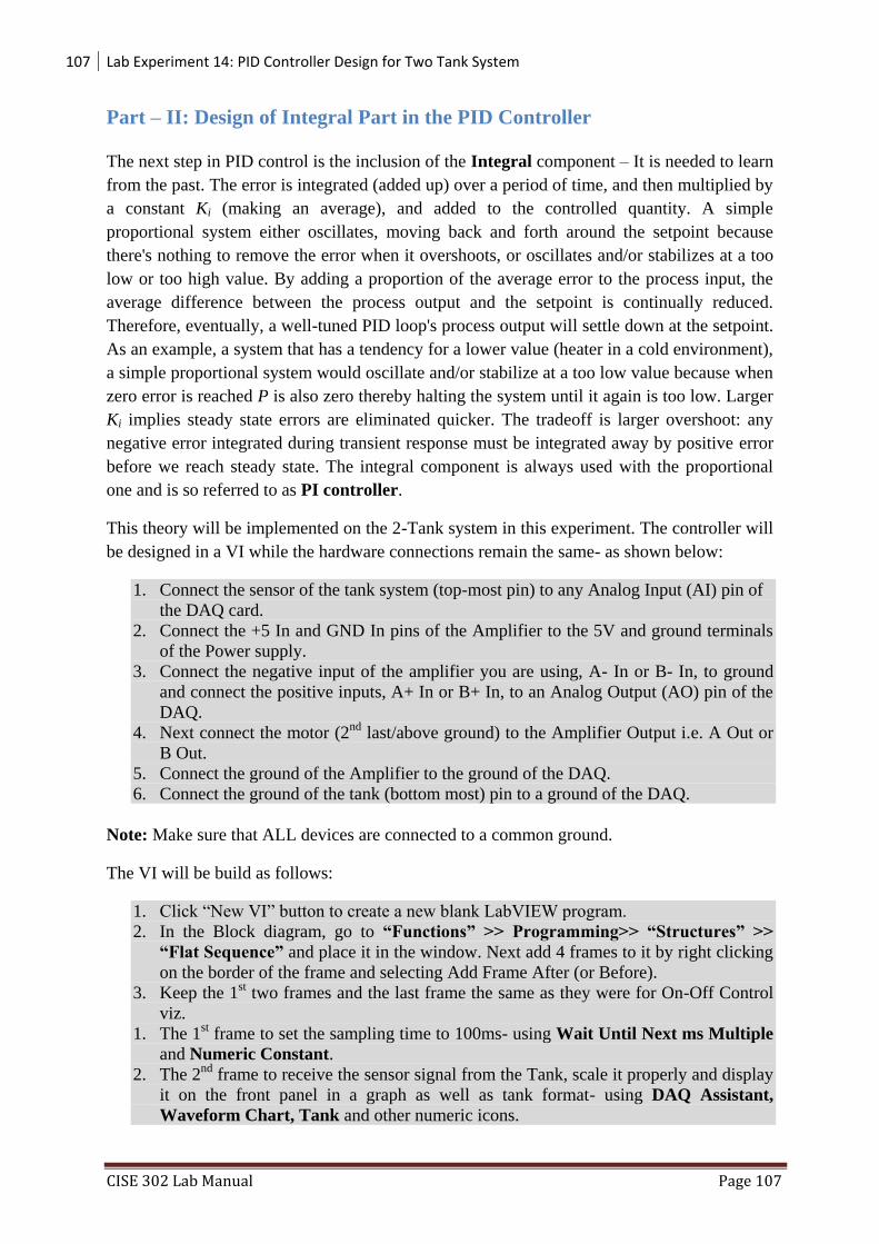
107 Lab Experiment 14: PID Controller Design for Two Tank System
CISE 302 Lab Manual Page 107
Part – II: Design of Integral Part in the PID Controller
The next step in PID control is the inclusion of the Integral component – It is needed to learn
from the past. The error is integrated (added up) over a period of time, and then multiplied by
a constant Ki (making an average), and added to the controlled quantity. A simple
proportional system either oscillates, moving back and forth around the setpoint because
there's nothing to remove the error when it overshoots, or oscillates and/or stabilizes at a too
low or too high value. By adding a proportion of the average error to the process input, the
average difference between the process output and the setpoint is continually reduced.
Therefore, eventually, a well-tuned PID loop's process output will settle down at the setpoint.
As an example, a system that has a tendency for a lower value (heater in a cold environment),
a simple proportional system would oscillate and/or stabilize at a too low value because when
zero error is reached P is also zero thereby halting the system until it again is too low. Larger
Ki implies steady state errors are eliminated quicker. The tradeoff is larger overshoot: any
negative error integrated during transient response must be integrated away by positive error
before we reach steady state. The integral component is always used with the proportional
one and is so referred to as PI controller.
This theory will be implemented on the 2-Tank system in this experiment. The controller will
be designed in a VI while the hardware connections remain the same- as shown below:
1. Connect the sensor of the tank system (top-most pin) to any Analog Input (AI) pin of
the DAQ card.
2. Connect the +5 In and GND In pins of the Amplifier to the 5V and ground terminals
of the Power supply.
3. Connect the negative input of the amplifier you are using, A- In or B- In, to ground
and connect the positive inputs, A+ In or B+ In, to an Analog Output (AO) pin of the
DAQ.
4. Next connect the motor (2nd
last/above ground) to the Amplifier Output i.e. A Out or
B Out.
5. Connect the ground of the Amplifier to the ground of the DAQ.
6. Connect the ground of the tank (bottom most) pin to a ground of the DAQ.
Note: Make sure that ALL devices are connected to a common ground.
The VI will be build as follows:
1. Click “New VI” button to create a new blank LabVIEW program.
2. In the Block diagram, go to “Functions” >> Programming>> “Structures” >>
“Flat Sequence” and place it in the window. Next add 4 frames to it by right clicking
on the border of the frame and selecting Add Frame After (or Before).
3. Keep the 1st two frames and the last frame the same as they were for On-Off Control
viz.
1. The 1st frame to set the sampling time to 100ms- using Wait Until Next ms Multiple
and Numeric Constant.
2. The 2nd
frame to receive the sensor signal from the Tank, scale it properly and display
it on the front panel in a graph as well as tank format- using DAQ Assistant,
Waveform Chart, Tank and other numeric icons.

108 Lab Experiment 14: PID Controller Design for Two Tank System
CISE 302 Lab Manual Page 108
3. The last frame to manually terminate the execution of the program through a stop
button on the front panel and make sure the motor is turned off at the end- using DAQ
Assistant, Case Structure and Numeric Constant.
4. (The entire Flat Sequence must be included in the while loop and the Stop button
terminal must be connected to the stop button of the while loop)
5. Calculate the Error by subtracting (“Functions” >> Programming>> “Numeric” >>
“Subtract”) the sensor value or level from the desired set point. The set point can be
given in the form of a Numeric Constant in the Block diagram or through Vertical
pointer slides, Numeric controls, etc. on the Front panel. This can be done in the 2nd
or
3rd
frame.
6. On the front panel, add 2 Control Knobs from the Numeric palette. This will be used
to control the Proportional gain Kp and the Integral Gain KI.
7. In the 3rd
frame of the Block diagram sequence, check if the error is less than zero. If
it is, then send the tank 0.If not go to the next step. The comparison can be made
using the Case Structure and the “Lesser Or Equal?” function.
8. Multiply the error with the gain by connecting the error and gain terminal to a
multiplication block. Also, integrate the error by sending it to the Integral block
(“Functions” >> Mathematics>> Integ & diff >>Time Domain Math- select
Integral in this block) and then multiply the integrated error with the Integral gain as
was done with the Proportional gain. Next, add the 2 products together (use
compound arithmetic or 2 add functions). Send the sum to the Tank through the DAQ
Assistant.
9. In the same frame check the above product (input to controller) and if it is greater than
1 send one to the Tank system- using DAQ. If it is lesser than 0 send the tank 0. If it is
between 0 and 1, send the control input as it is. The comparison can be done using
“Greater Or Equal?” and “Lesser Or Equal?” functions along with a Case Structure
having another Case Structure inside (as in the On-Off Control). Here the control
input is connected to the Case Selector.
10. In the 2-Tank system open the exit valve a little to see the proper effect of the PI
Control. The valve can be opened to the number 2 position or another one depending
on the speed of the motor.
11. After all the wiring is complete switch to Front Panel and press the RUN button to
execute the VI.