cis 2033 lectures 3 and 4, spring 2017 - github pages · cis 2033 lectures 3 and 4, spring 2017 2...

CIS 2033 Lectures 3 and 4, Spring 201711 Supplemental reading from Dekking’stextbook: Chapter 3.

Instructor: David DoborUpdated January 24, 2017

In the first two lectures, we introduced probabilities as a way of de-scribing our beliefs about the likelihood that a given event will occur.But our beliefs will in general depend on the information that we have.Taking into account new information leads us to consider the so-calledconditional probabilities – revised probabilities that take into accountthis new information.

Conditional probabilities are very useful whenever we want tobreak up a model into simpler pieces using a divide and conquerstrategy. This is done using tools that we develop in this lecture andwhich we will keep applying throughout this course in different guises.They are also the foundation of the field of inference, and we will seehow they arise in that context as well.

Next, we will consider a special case where one event does not con-vey useful information about another, a situation that we call indepen-dence. Independence usually describes a situation where the occurrenceor non-occurrence of different events is determined by factors that arecompletely unrelated. Independence is what allows us to build com-plex models out of simple ones. This is because it is often the case thata complex system is made up of several components that are affectedby unrelated, that is, independent sources of randomness.

And so with the tools to be developed over the next couple of lec-tures, we will be ready to calculate probabilities in fairly complexprobabilistic models.

Introduction

Suppose I look at the registry of residents of my town and pick aperson at random. What is the probability that this person is under18 years of age? Let’s say I find that the answer is about 25%.

Suppose now that I tell you that this person is married. Will yougive the same answer? Of course not. The probability of being lessthan 18 years old is now much smaller.

What happened here? We started with some initial probabilitiesthat reflect what we know or believe about the world. But we thenacquired some additional knowledge, some new evidence– for exam-ple, about this person’s family situation. This new knowledge shouldcause our beliefs to change, and the original probabilities must bereplaced with new probabilities that take into account the new in-formation. These revised probabilities are what we call conditionalprobabilities. And this is the subject of this lecture.

We will start with a formal definition of conditional probabilitiestogether with the motivation behind this particular definition. Wewill then proceed to develop three tools that rely on conditional

cis 2033 lectures 3 and 4, spring 2017 2

probabilities, including the Bayes rule, which provides a systematicway for incorporating new evidence into a probability model. Thethree tools that we introduce in this lecture involve very simple andelementary mathematical formulas, yet they encapsulate some verypowerful ideas.

It is not an exaggeration to say that much of this class will revolvearound the repeated application of variations of these three toolsto increasingly complicated situations. In particular, the Bayes ruleis the foundation for the field of inference. It is a guide on how toprocess data and make inferences about unobserved quantities orphenomena. As such, it is a tool that is used all the time, all overscience and engineering.


Conditional Probabilities

Conditional probabilities are probabilities associated with a revisedmodel that takes into account some additional information about theoutcome of a probabilistic experiment. The question is how to carryout this revision of our model. We will give a mathematical definitionof conditional probabilities, but first let us motivate this definition byexamining a simple concrete example.

Example 1. Consider a probability model with 12 equally likelypossible outcomes – each outcome has probability equal to 1/12. Wewill focus on two particular events, event A and B, two subsets of thesample space. Event A has five elements, so its probability is 5/12,and event B has six elements, so it has probability 6/12.

Figure 1: Equally Likely Outcomes.In this model with equally likelyoutcomes, the probabilities associatedwith sets A and B are 5/12 and 1/2,respectively.

Figure 2: Event B has occurred. Ifis known that B has occurred, wenow update our model by assigning0 probability to the events that areoutside of B.

Suppose now that someone tells you that event B has occurred,but tells you nothing more about the outcome. How should the modelchange? First, those outcomes that are outside event B are no longerpossible. So we can either eliminate them, as was done in Figure 2, orwe might keep them in the picture but assign them 0 probability, sothat they cannot occur.

How about the outcomes inside the event B? We’re told that oneof these 6 outomes inside the event B has occurred. Now these 6

outcomes were equally likely in the original model, and there is noreason to change their relative probabilities. So they should remainequally likely in revised model as well, so each one of them shouldhave now probability 1/6 since there’s 6 of them. And this is ourrevised model, the conditional probability law:

0 probability to outcomes outside B, and probability 1/6 to each one of theoutcomes that is inside the event B.

Let us write now this down mathematically. We will use the no-tation P(A | B) to describe the conditional probability of an event Agiven that some other event B is known to have occurred. We readthis expression as probability of A given B.

So what are these conditional probabilities in our example? Inthe new model, where these outcomes are equally likely, we knowthat event A can occur in two different ways. Each one of them hasprobability 1/6. So the probability of event A is 2/6 (i.e. 1/3).

How about event B. Well, B consists of 6 possible outcomes eachwith probability 1/6. So event B in this revised model should haveprobability equal to 1. Of course, this is just saying the obvious.Given that we already know that B has occurred, the probabilitythat B occurs in this new model should be equal to 1.


Figure 3: Sample Space for Example2. The probability distribution here issuch that each individual outcome isnot necessarily equally likely.

Example 2. In this example, the sample space does not consist ofequally likely outcomes, but instead we’re given the probabilities ofdifferent pieces of the sample space. Notice here that the probabilitiesare consistent with what was used in the original example. So thispart of A that lies outside B has probability 3/12, but in this case I’mnot telling you how that probability is made up. I’m not telling youthat it consists of 3 equally likely outcomes. So all I’m telling you isthat the collective probability in the blue region in Figure 3 is 3/12.

The total probability of A is, again, 5/12 as before. The total prob-ability of B is 2/12 + 4/12 = 6/12, exactly as before. So it’s a sort ofsimilar situation as before. How should we revise our probabilitiesand create – construct – conditional probabilities once we are toldthat event B has occurred?

First, the relation P(B | B) = 1 should remain true: once we aretold that B has occurred, then B is certain to occur, so it should haveconditional probability equal to 1.

How about the conditional probability P(A | B)? Well, we can rea-son as follows. In the original model, and if we just look inside eventB, those outcomes that make event A happen had a collective prob-ability which was 1/3 of the total probability assigned to B (because2/12 is one-third of 2/12 + 4/12). So out of the overall probabilityassigned to B, 1/3 of that probability corresponds to outcomes inwhich event A is happening. Therefore, if I tell you that B has oc-curred, I should assign probability equal to 1/3 that event A is alsogoing to happen. So that P(A | B) should be equal to 1/3.

Check Your Understanding: Are the following statements true offalse?

1. If Ω is finite and we have a discrete uniform probability law, andif B 6= ∅, then the conditional probability law on B, given that Boccurred, is also discrete uniform.

2. If Ω is finite and we have a discrete uniform probability law, andif B 6= ∅, then the conditional probability law on Ω, given that Boccurred, is also discrete uniform.

(1)True,becausetheoutcomesinsideBmaintainthesamerelativeproportionsasintheoriginalprobabilitylaw.

(2)False.OutcomesinΩthatareoutsideBhavezeroconditionalprobability,soitcannotbethecasethatalloutcomesinΩhavethesameconditionalprobability.


Definition of Conditional Probability

By now, we should be satisfied that this approach is a reasonable wayof constructing conditional probabilities. But now let us translate ourreasoning into a formula. So we wish to come up with a formula thatgives us the conditional probability of an event given another event.

The particular formula that captures our way of thinking, as moti-vated before, is the following. Out of the total probability assigned toB, we ask the question, which fraction of that probability is assignedto outcomes under which event A also happens? So we are livinginside event B, but within that event, we look at those outcomes forwhich event A also happens – which is the intersection of A and B– and we ask: out of the total probability of B, what fraction of thatprobability is allocated to that intersection of A with B?

So the following formula captures our intuition of what we didbefore to construct conditional probabilities in examples 1 and 2.

Let us check that the definition indeed does what it’s supposed todo. In this example, the probability of the intersection was 2/12 andthe total probability of B was 6/12, which gives us 1/3, which is theanswer that we had gotten intuitively a little earlier.

As a side point, let me also make a comment that this definitionof conditional probabilities makes sense only if we do not attempt todivide by zero, i.e. only if the event B on which we’re conditioninghas positive probability. If event B has 0 probability, then conditionalprobabilities given B will be left undefined.

And one final comment. This is a definition. It’s not a theorem.What does that mean? It means that there is no question whetherthis equality is correct or not. It’s just a definition. There’s no issue ofcorrectness. The earlier argument that we gave was just a motivationof the definition. We tried to figure out what the definition should beif we want to have a certain intuitive and meaningful interpretationof the conditional probabilities. Let us now continue with a simpleexample.

Example 3. This is a example where we want to just apply the for-mula for conditional probabilities and see what we get. The example


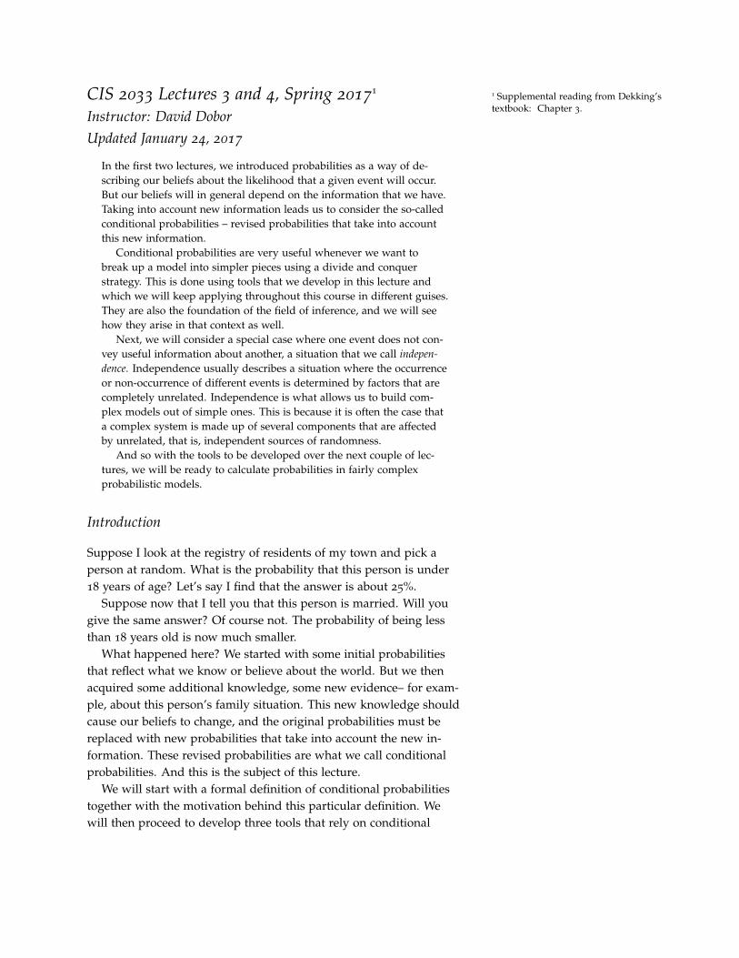
involves a four-sided die, which we roll twice, and we record thefirst roll, and the second roll. So there are 16 possible outcomes. Weassume, to keep things simple, that each one of those 16 possible out-comes has the same probability, so each outcome has the probability1/16.

Figure 4: Tetrahedral die, again.

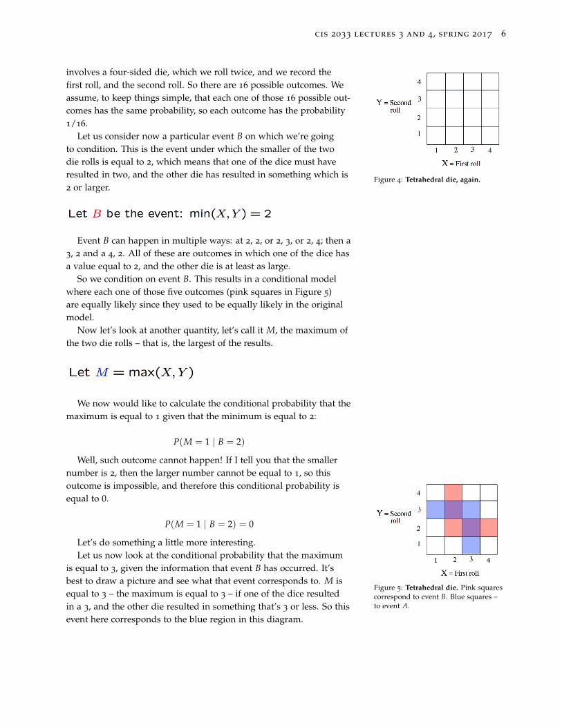
Let us consider now a particular event B on which we’re goingto condition. This is the event under which the smaller of the twodie rolls is equal to 2, which means that one of the dice must haveresulted in two, and the other die has resulted in something which is2 or larger.

Event B can happen in multiple ways: at 2, 2, or 2, 3, or 2, 4; then a3, 2 and a 4, 2. All of these are outcomes in which one of the dice hasa value equal to 2, and the other die is at least as large.

So we condition on event B. This results in a conditional modelwhere each one of those five outcomes (pink squares in Figure 5)are equally likely since they used to be equally likely in the originalmodel.

Now let’s look at another quantity, let’s call it M, the maximum ofthe two die rolls – that is, the largest of the results.

We now would like to calculate the conditional probability that themaximum is equal to 1 given that the minimum is equal to 2:

P(M = 1 | B = 2)

Well, such outcome cannot happen! If I tell you that the smallernumber is 2, then the larger number cannot be equal to 1, so thisoutcome is impossible, and therefore this conditional probability isequal to 0.

P(M = 1 | B = 2) = 0

Let’s do something a little more interesting.

Figure 5: Tetrahedral die. Pink squarescorrespond to event B. Blue squares –to event A.

Let us now look at the conditional probability that the maximumis equal to 3, given the information that event B has occurred. It’sbest to draw a picture and see what that event corresponds to. M isequal to 3 – the maximum is equal to 3 – if one of the dice resultedin a 3, and the other die resulted in something that’s 3 or less. So thisevent here corresponds to the blue region in this diagram.


Now let us try to calculate the conditional probability by just fol-lowing the definition. The conditional probability of one event givenanother is the probability that both of the two events occur, dividedby the probability of the conditioning event. That is, out of the totalprobability in the conditioning event, we ask, what fraction of thatprobability is assigned to outcomes in which the event of interest isalso happening?

So what is this event? The maximum is equal to 3, which is theblue event. And simultaneously, the pink event is happening. Thesetwo events intersect only in two places. Figure 5 shows the intersec-tion of the two events - these are the squares that are shaded bothblue and pink. And the probability of that intersection is 2 out of 16,since there are 16 outcomes and that event happens only with twoparticular outcomes. So this gives us 2/16 in the numerator.

How about the denominator? Event B consists of a total of fivepossible outcomes. Each one has probability 1/16, so this is 5/16.Thus the final answer is 2/16 divided by 5/16, or 2/5.

We could have gotten that same answer in a simple and perhapsmore intuitive way. In the original model, all outcomes were equallylikely. Therefore, in the conditional model, the five outcomes thatbelong to B should also be equally likely. Out of those five, there aretwo of them that make the event of interest to occur. So given that welive in B, there’s two ways out of five that the event of interest willmaterialize. So the event of interest has conditional probability equalto 2/5.

Check Your Understanding: Let the sample space be the unit square,Ω = [0, 1]2, and and let the probability of a set be the area of the set.Let A be the set of points (x, y) ∈ [0, 1]2 for which y ≤ x. Let B be theset of points for which x ≤ 1/2. Find P(A | B).

theanswerisonefourth

Conditional Probabilities Obey the Same Axioms

(Skim this section on first reading.)

We want to emphasize an important point. Conditional probabili-ties are just the same as ordinary probabilities applied to a differentsituation. They do not taste or smell or behave any differently thanordinary probabilities. What do I mean by that? Figure 6: Conditional probabilities also

satisfy the familiar axioms. This onewas axiom 1.Axiom 1. I mean that they satisfy the usual probability axioms. For

example, ordinary probabilities must be non-negative. Is this truefor conditional probabilities? Of course it is true, because conditional


probabilities are defined as a ratio of two probabilities. Probabilitiesare non-negative. So the ratio will also be non-negative, of course aslong as it is well-defined. And here we need to remember that weonly talk about conditional probabilities when we condition on anevent that itself has positive probability.

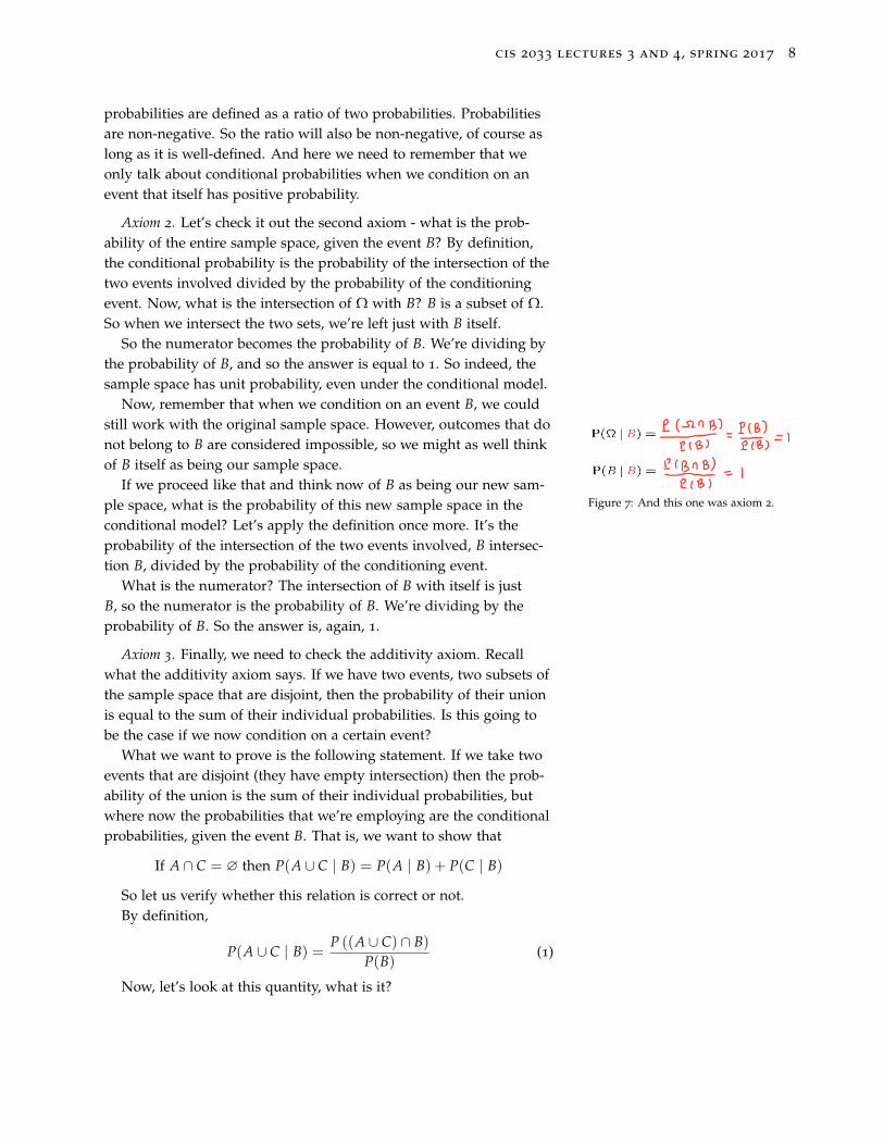
Axiom 2. Let’s check it out the second axiom - what is the prob-ability of the entire sample space, given the event B? By definition,the conditional probability is the probability of the intersection of thetwo events involved divided by the probability of the conditioningevent. Now, what is the intersection of Ω with B? B is a subset of Ω.So when we intersect the two sets, we’re left just with B itself.

So the numerator becomes the probability of B. We’re dividing bythe probability of B, and so the answer is equal to 1. So indeed, thesample space has unit probability, even under the conditional model.

Now, remember that when we condition on an event B, we couldstill work with the original sample space. However, outcomes that donot belong to B are considered impossible, so we might as well thinkof B itself as being our sample space.

Figure 7: And this one was axiom 2.If we proceed like that and think now of B as being our new sam-

ple space, what is the probability of this new sample space in theconditional model? Let’s apply the definition once more. It’s theprobability of the intersection of the two events involved, B intersec-tion B, divided by the probability of the conditioning event.

What is the numerator? The intersection of B with itself is justB, so the numerator is the probability of B. We’re dividing by theprobability of B. So the answer is, again, 1.

Axiom 3. Finally, we need to check the additivity axiom. Recallwhat the additivity axiom says. If we have two events, two subsets ofthe sample space that are disjoint, then the probability of their unionis equal to the sum of their individual probabilities. Is this going tobe the case if we now condition on a certain event?

What we want to prove is the following statement. If we take twoevents that are disjoint (they have empty intersection) then the prob-ability of the union is the sum of their individual probabilities, butwhere now the probabilities that we’re employing are the conditionalprobabilities, given the event B. That is, we want to show that

If A ∩ C = ∅ then P(A ∪ C | B) = P(A | B) + P(C | B)

So let us verify whether this relation is correct or not.By definition,

P(A ∪ C | B) =P ((A ∪ C) ∩ B)

P(B)(1)

Now, let’s look at this quantity, what is it?


We take the union A ∪ C, and then intersect it with B. The resultconsists of the two gray pieces in Figure 8 .

Figure 8: And this picture illustratesaxiom 3 for conditional probabilities.

So we rewrite expression (1) as follows:

P(A ∪ C | B) =P ((A ∪ C) ∩ B)

P(B)

=P ((A ∩ B) ∪ (C ∩ B))

P(B)

OK, now here’s an observation. We assumed that the events A andC were disjoint. Then the piece of A that also belongs in B, therefore,is disjoint from the piece of C that also belongs to B.

Since A ∩ B and C ∩ B are disjoint, the probability of their unionhas to be equal to the sum of their individual probabilities. So herewe’re using the additivity axiom on the original probabilities to breakthis probability up into two pieces.

Thus we continue the previous expression as follows:

P ((A ∩ B) ∪ (C ∩ B))P(B)

=P(A ∩ B) + P(C ∩ B)

P(B)

=P(A ∩ B)

P(B)+

P(C ∩ B)P(B)

And now we observe that here we have ratios of probabilities ofintersections by the probability of B. So we see that the first termis just the conditional probability P(A | B), using the definition ofconditional probabilities. Similarly, the second part is just P(C | B).

So we have indeed checked that this additivity property is true forthe case of conditional probabilities when we consider two disjointevents.

Now, we could repeat the same derivation and verify that it isalso true for the case of a disjoint union of finitely many events, oreven for countably many disjoint events. We’re not proving it, but theargument is exactly the same as for the case of two events.

To conclude, conditional probabilities do satisfy all of the standardaxioms of probability theory. So conditional probabilities are just likeordinary probabilities.

This actually has a very important implication. Since conditionalprobabilities satisfy all of the probability axioms, any formula ortheorem that we ever derive for ordinary probabilities will remaintrue for conditional probabilities as well.


Models Based on Conditional Probabilities

Let us now examine what conditional probabilities are good for. Wehave already discussed that they are used to revise a model when weget new information, but there is another way in which they arise.We can use conditional probabilities to build a multi-stage model ofa probabilistic experiment. We will illustrate this through an exampleinvolving the detection of an object up in the sky by a radar. We willkeep our example very simple. On the other hand, it turns out tohave all the basic elements of a real-world model.

So, we are looking up in the sky, and either there’s an airplaneflying up there or not. Let us call Event A the event that an airplaneis indeed flying up there:

Event A : Airplane is flying above,

and we have two possibilities: either event A occurs, or the comple-ment of A occurs, in which case nothing is flying up there. At thispoint, we can also assign some probabilities to these two possibili-ties. Let us say that through prior experience, perhaps, or some otherknowledge, we know that the probability that something is indeedflying up there is 5% and with probability 95% nothing is flying.

Now, we also have a radar that looks up into the sky. Let event Bbe that the radar detects something:

Event B : Something registers on the radar screen

There are two things that can happen: either something registerson the radar screen or nothing registers. Of course, if it’s a goodradar, probably event B will tend to go together with event A. But it’salso possible that the radar will make some mistakes.

And so we have various possibilities. If there’s a plane up there,it’s possible that the radar will detect it, in which case event B willalso happen. But it’s also conceivable that the radar will not detect it,in which case we have a so-called miss. So "miss" happens if a planeis flying up there, but the radar does not detect it.

Figure 9: Event A ∩ Bc is called a "miss".Event Ac ∩ B is called a "false alarm".Pause here a second and make sure thisterminology makes sense to you.

Another possibility is that nothing is flying up there, but the radardoes detect something, and this is a situation that’s called a falsealarm. Finally, there’s the possibility that nothing is flying up there,and the radar did not see anything either.


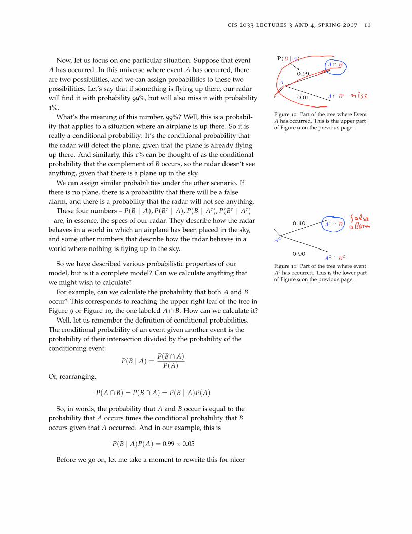
Figure 10: Part of the tree where EventA has occurred. This is the upper partof Figure 9 on the previous page.

Now, let us focus on one particular situation. Suppose that eventA has occurred. In this universe where event A has occurred, thereare two possibilities, and we can assign probabilities to these twopossibilities. Let’s say that if something is flying up there, our radarwill find it with probability 99%, but will also miss it with probability1%.

What’s the meaning of this number, 99%? Well, this is a probabil-ity that applies to a situation where an airplane is up there. So it isreally a conditional probability: It’s the conditional probability thatthe radar will detect the plane, given that the plane is already flyingup there. And similarly, this 1% can be thought of as the conditionalprobability that the complement of B occurs, so the radar doesn’t seeanything, given that there is a plane up in the sky.

We can assign similar probabilities under the other scenario. Ifthere is no plane, there is a probability that there will be a falsealarm, and there is a probability that the radar will not see anything.

These four numbers – P(B | A), P(Bc | A), P(B | Ac), P(Bc | Ac)

– are, in essence, the specs of our radar. They describe how the radarbehaves in a world in which an airplane has been placed in the sky,and some other numbers that describe how the radar behaves in aworld where nothing is flying up in the sky.

Figure 11: Part of the tree where eventAc has occurred. This is the lower partof Figure 9 on the previous page.

So we have described various probabilistic properties of ourmodel, but is it a complete model? Can we calculate anything thatwe might wish to calculate?

For example, can we calculate the probability that both A and Boccur? This corresponds to reaching the upper right leaf of the tree inFigure 9 or Figure 10, the one labeled A∩ B. How can we calculate it?

Well, let us remember the definition of conditional probabilities.The conditional probability of an event given another event is theprobability of their intersection divided by the probability of theconditioning event:

P(B | A) =P(B ∩ A)

P(A)

Or, rearranging,

P(A ∩ B) = P(B ∩ A) = P(B | A)P(A)

So, in words, the probability that A and B occur is equal to theprobability that A occurs times the conditional probability that Boccurs given that A occurred. And in our example, this is

P(B | A)P(A) = 0.99× 0.05

Before we go on, let me take a moment to rewrite this for nicer


looks. (Heads up: It helps on quizzes to know these nside out.) Wehave:

So we can calculate the probability of event A ∩ B by multiplyingprobabilities and conditional probabilities along the path in the treediagram that leads us to the top right leaf.

Figure 12: The branches leading toevent A ∩ B are traced in red.

And we can do the same for any other leaf in this diagram. Sofor example, the probability that Ac ∩ Bc happens is going to be theprobability event Ac times the conditional probability P(Bc | Ac).

So you could trace these two branches too to get the probability0.95 × 0.90 = 0.855 of event Ac ∩ Bc occurring.

How about a different question? What is the probability, the totalprobability, that the radar sees something? Let us try to identify thisevent. The radar can see something under two scenarios:

1. A plane is up in the sky and the radar sees it.

2. Nothing is up in the sky, but the radar thinks that it sees some-thing.

These two possibilities together make up the event B.

And so to calculate the probability of B, we need to add the proba-bilities of these two events.

For the first event, we already calculated its probability. It’s 0.05 ×0.99. For the second possibility, we need to do a similar calculation.The probability that this second event occurs is equal to 0.95 timesthe conditional probability of B occurring under the scenario whereAc has occurred, and this is 0.10. So we have P(Ac ∩ B) = 0.95 ×0.10.

We add those two numbers together, the answer turns out to be:

P(B) = P(A)P(B | A) + P(Ac)P(B | Ac)

= 0.05× 0.99 + 0.95× 0.10

= 0.1445

Finally, the last question, which is perhaps the most interestingone. Suppose that the radar registered something. What is the prob-ability that there is an airplane up there? How do we do this cal-culation? Well, we can start from the definition of the conditional


probability of A given B, and note that we already have in our handsboth the numerator and the denominator.

P(A | B) =P(A ∩ B)

P(B)

=0.05× 0.99

0.05× 0.99 + 0.95× 0.10

=0.04950.1445

= 0.3426

So there is a 34% probability that an airplane is there given thatthe radar has seen or thinks that it sees something.

Now, the numerical value of this answer is somewhat interesting be-cause it’s pretty small. Even though we have a very good radar thattells us the right thing 99% of the time under one scenario and 90%under the other scenario. Despite that, given that the radar has seensomething, this is not really convincing or compelling evidence thatthere is an airplane up there. The probability that there’s an airplaneup there is only 34% in a situation where the radar thinks that it hasseen something.

In the next few segments, we are going to revisit these three cal-culations and see how they can generalize. In fact, a large part ofwhat is to happen in the remainder of this class will be elaborationon these three ideas. They are three types of calculations that willshow up over and over, of course, in more complicated forms, but thebasic ideas are essentially captured in this simple example.


Multiplication Rule

As promised, we will now start developing generalizations of thedifferent calculations that we carried out in the context of the radarexample. The first kind of calculation that we carried out goes underthe name of the multiplication rule. And it goes as follows. Ourstarting point is the definition of conditional probabilities.

The conditional probability of A given another event, B, is theprobability that both events have occurred divided by the probabilityof the conditioning event.

P(A | B) =P(A ∩ B)

P(B)

We now take the denominator term and send it to the other side ofthis equality to obtain this relation

P(A ∩ B) = P(A | B)P(B)

which we can interpret as follows. The probability that two eventsoccur is equal to the probability that a first event occurs, event B inthis case, times the conditional probability that the second event,event A, occurs, given that event B has occurred.

Now, out of the two events, A and B, we’re of course free tochoose which one we call the first event and which one we call thesecond event. So the probability of the two events happening is alsoequal to an expression of this form

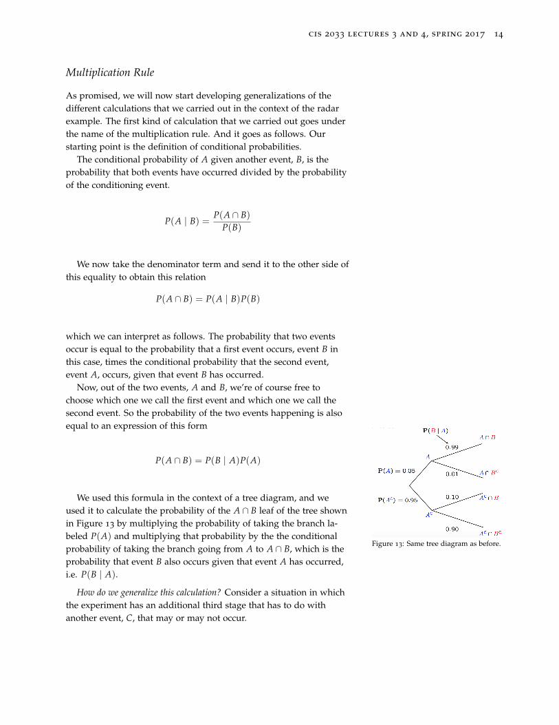
P(A ∩ B) = P(B | A)P(A)

Figure 13: Same tree diagram as before.

We used this formula in the context of a tree diagram, and weused it to calculate the probability of the A ∩ B leaf of the tree shownin Figure 13 by multiplying the probability of taking the branch la-beled P(A) and multiplying that probability by the the conditionalprobability of taking the branch going from A to A ∩ B, which is theprobability that event B also occurs given that event A has occurred,i.e. P(B | A).

How do we generalize this calculation? Consider a situation in whichthe experiment has an additional third stage that has to do withanother event, C, that may or may not occur.


Figure 14: Here our experiment has thethird stage that has to do with anotherevent C.

For example, if we have arrived at the node labeled A ∩ B, A andB have both occurred. Next, if C also occurs, then we reach the leaf ofthe tree that is labeled A ∩ B ∩ C. Or there could be other scenarios.For example, it could be the case that A did not occur. Then event Boccurred, and finally, event C did not occur, in which case we end upat the leaf labeled Ac ∩ B ∩ Cc.

What is the probability of this scenario happening? Let us tryto do a calculation similar to the one that we used for the case oftwo events. However, we need to deal here with three events. Whatshould we do? Well, we look at the intersection of these three eventsand think of it as the intersection of a composite event, Ac ∩ B, thenintersected with the event Cc.

P(Ac ∩ B ∩ Cc) = P ((Ac ∩ B) ∩ Cc)

Clearly, you can form the intersection of three events by first tak-ing the intersection of two of them and then intersecting with a third.After we group things this way, we’re dealing with the probability oftwo events happening, the composite event(Ac ∩ B) and the ordinaryevent Cc. And the probability of two events happening is equal to theprobability that the first event happens, and then the probability thatthe second event happens, given that the first one has happened.

P ((Ac ∩ B) ∩ Cc) = P(Ac ∩ B) P(Cc | Ac ∩ B)

Can we simplify this even further? Yes. The first term is the prob-ability of two events happening. So it can be simplified further as theprobability that Ac occurs times the conditional probability that Boccurs, given that Ac has occurred. And then we carry over the lastterm exactly the way it is.

P(Ac ∩ B ∩ Cc) = P(Ac ∩ B) P(Cc | Ac ∩ B)

= P(Ac) P(B | A) P(Cc | Ac ∩ B)

The conclusion is that we can calculate the probability of theleaf labeled Ac ∩ B ∩ Cc by multiplying the probabilities of the redbranches shown in figure 15. Figure 15: Lower part of the same tree

as in Figure 14. We multiply the prob-abilities associated with the branchestraced in red to get the probability ofthe event Ac ∩ B ∩ Cc.

At this point, you can probably see that such a formula shouldalso be valid for the case of more than three events. The probabilitythat a bunch of events all occur should be the probability of the firstevent times a number of factors, each corresponding to a branch in atree of this kind.

In particular, the probability that events A1, A2, . . . An all occur is


going to be

P(A1 ∩ A2 ∩ . . . An) = P(A1)n

∏i=2

P(Ai | A1 ∩ . . . ∩ Ai−1) (2)

This is the most general version of the multiplication rule andallows you to calculate the probability of several events happening bymultiplying probabilities and conditional probabilities.

Check Your Understanding: Are the following statements true orfalse? (Assume that all conditioning events have positive probability.)

1. P(A ∩ B ∩ Cc) = P(A ∩ B)P(Cc | A ∩ B)

2. P(A ∩ B ∩ Cc) = P(A)P(Cc | A)P(B | A ∩ Cc)

3. P(A ∩ B ∩ Cc) = P(A)P(Cc ∩ A | A)P(B | A ∩ Cc)

4. P(A ∩ B | C) = P(A | C)P(B | A ∩ C)

1.ThisistheusualmultipicationruleappliedtothetwoeventsA∩BandCc.True.

2.Thisistheusualmultiplicationrule.Inequation(2)above,considerthesequenceofeventsA,Cc,andB.True.

3.Thisisbecause

P(Cc∩A|A)=P(Cc∩A∩A)

P(A)=

P(Cc∩A)

P(A)=P(Cc|A).

So,thisstatementisequivalenttotheoneinpart2.True.

4.ThisistheusualmultiplicationruleP(A∩B)=P(A)P(B|A),appliedtoamodel/universeinwhicheventCisknowntohaveoccurred.True.

The Total Probability Theorem

Let us now revisit the second calculation that we carried out in thecontext of our earlier example. In that example, we calculated thetotal probability of an event that can occur under different scenarios.And it involves the powerful idea of divide and conquer where webreak up complex situations into simpler pieces.

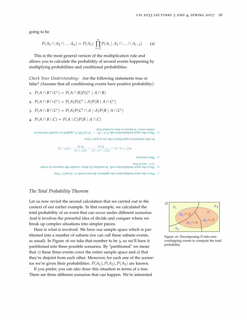
Figure 16: Decomposing Ω into non-overlapping events to compute the totalprobability.

Here is what is involved. We have our sample space which is par-titioned into a number of subsets (we can call these subsets events,as usual). In Figure 16 we take that number to be 3, so we’ll have itpartitioned into three possible scenarios. By "partitioned" we meanthat 1) these three events cover the entire sample space and 2) thatthey’re disjoint from each other. Moreover, for each one of the scenar-ios we’re given their probabilities: P(A1), P(A2), P(A3) are known.

If you prefer, you can also draw this situation in terms of a tree.There are three different scenarios that can happen. We’re interested


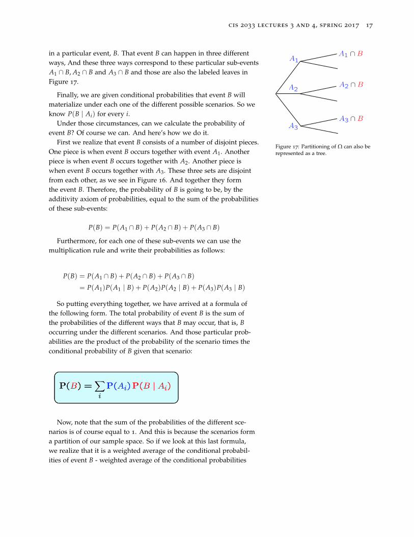
in a particular event, B. That event B can happen in three differentways, And these three ways correspond to these particular sub-eventsA1 ∩ B, A2 ∩ B and A3 ∩ B and those are also the labeled leaves inFigure 17.

Figure 17: Partitioning of Ω can also berepresented as a tree.

Finally, we are given conditional probabilities that event B willmaterialize under each one of the different possible scenarios. So weknow P(B | Ai) for every i.

Under those circumstances, can we calculate the probability ofevent B? Of course we can. And here’s how we do it.

First we realize that event B consists of a number of disjoint pieces.One piece is when event B occurs together with event A1. Anotherpiece is when event B occurs together with A2. Another piece iswhen event B occurs together with A3. These three sets are disjointfrom each other, as we see in Figure 16. And together they formthe event B. Therefore, the probability of B is going to be, by theadditivity axiom of probabilities, equal to the sum of the probabilitiesof these sub-events:

P(B) = P(A1 ∩ B) + P(A2 ∩ B) + P(A3 ∩ B)

Furthermore, for each one of these sub-events we can use themultiplication rule and write their probabilities as follows:

P(B) = P(A1 ∩ B) + P(A2 ∩ B) + P(A3 ∩ B)

= P(A1)P(A1 | B) + P(A2)P(A2 | B) + P(A3)P(A3 | B)

So putting everything together, we have arrived at a formula ofthe following form. The total probability of event B is the sum ofthe probabilities of the different ways that B may occur, that is, Boccurring under the different scenarios. And those particular prob-abilities are the product of the probability of the scenario times theconditional probability of B given that scenario:

Now, note that the sum of the probabilities of the different sce-narios is of course equal to 1. And this is because the scenarios forma partition of our sample space. So if we look at this last formula,we realize that it is a weighted average of the conditional probabil-ities of event B - weighted average of the conditional probabilities


where the probabilities of the individual scenarios are the weights.In words, the probability that an event occurs is a weighted averageof the probability that it has under each possible scenario, where theweights are the probabilities of the different scenarios.

One final comment– our derivation was for the case of threeevents. But you can certainly see that the same derivation wouldgo through if we had any finite number of events. But even more, ifwe had a partition of our sample space into an infinite sequence ofevents, the same derivation would still go through, except that in thisplace in the derivation, instead of using the ordinary additivity ax-iom we would have to use the countable additivity axiom. But otherthan that, all the steps would be the same. And we would end upwith the same formula, except that now we would have an infinitesum over the infinite set of scenarios.

Check Your Understanding: We have an infinite collection of biasedcoins, indexed by the positive integers. Coin i has probability 2−i ofbeing selected. A flip of coin i results in Heads with probability 3−i.We select a coin and flip it. What is the probability that the result isHeads?

The geometric sum formula may be useful here: ∑∞i=1 αi = α

1−α ,when |α| < 1.

theanswerisonefifth.Wethinkoftheselectionofcoiniasscenario/eventAi.Bythetotalprobabilitytheorem,forthecaseofinfinitelymanyscenarios,

P(Heads)=∞

∑i=1P(Ai)P(Heads|Ai)=

∞

∑i=12−i3−i=

∞

∑i=1(1/6)i=1/6

1−(1/6).


The Bayes Rule

We now come to the third and final kind of calculation out of thecalculations that we carried out in our earlier example. The setting isexactly the same as in our discussion of the total probability theorem.We have a sample space which is partitioned into a number of dis-joint subsets, or events, which we think of as scenarios. We’re giventhe probability of each scenario.

Figure 18: The setting is exactly thesame as in our calculations of totalprobability.

And we think of these probabilities Ai as being some kind of ini-tial beliefs. They capture how likely we believe each scenario to be.Now, under each scenario, we also have the probability that an eventof interest, event B, will occur. Then the probabilistic experiment iscarried out, and we observe that event B did indeed occur.

Once that happens, maybe this should cause us to revise our be-liefs about the likelihood of the different scenarios. Having observedthat B occurred, perhaps certain scenarios are more likely than oth-ers. How do we revise our beliefs? By calculating conditional proba-bilities.

And how do we calculate conditional probabilities? We start fromthe definition of conditional probabilities. The probability of oneevent given another is the probability that both events occur dividedby the probability of the conditioning event:

P(Ai | B) =P(Ai ∩ B)

P(B)

How do we continue? We simply realize that the numerator iswhat we can calculate using the multiplication rule. And the denomi-nator is exactly what we calculate using the total probability theorem.So we have everything we need to calculate those revised beliefs, i.e.conditional probabilities.

And this is all there is in the Bayes rule. It is actually a very simplecalculation. However, it is a quite important one.

Its history goes way back. In the middle of the 18th century, aPresbyterian minister, Thomas Bayes, worked it out. It was publisheda few years after his death and was quickly reorganized for its signif-icance.

Bayes rule is a systematic way for incorporating new evidence, forlearning from experience. And it forms the foundation of a major


branch of mathematics, so-called Bayesian inference, which we willstudy in some detail later in this course.

The general idea of Bayesian inference is that we start with a prob-abilistic model which involves a number of possible scenarios, Ai,and we have some initial beliefs, P(Ai), on the likelihood of eachpossible scenario.

There’s also some particular event B that may occur under eachscenario. And we know how likely it is to occur under each scenario.

We then actually observe that B occurred, and then we use thatinformation to draw conclusions about the possible causes of B, orconclusions about the more likely or less likely scenarios that mayhave caused this events to occur. That is, having observed B, wemake inferences as to how likely a particular scenario, say Ai, is go-ing to be. That likelihood is captured by the conditional probabilitiesof Ai, given the event B, that is, by P(Ai | B).

That’s exactly what inference is all about, as we’re going to seelater in this class.

Check Your Understanding: A test for a certain rare disease is as-sumed to be correct 95% of the time: if a person has the disease, thetest result is positive with probability 0.95, and if the person does nothave the disease, the test result is negative with probability 0.95. Aperson drawn at random from a certain population has probability0.001 of having the disease.

1. Find the probability that a random person tests positive.

2. Given that the person just tested positive, what is the probabilityhe actually has the disease?

Let A be the event that the person has the disease, and B the event that the test result is positive.

1. The desired probability is

P(B) = P(A)P(B | A) + P(Ac)P(B | Ac) = 0.001× 0.95 + 0.999× 0.05 = 0.0509

2. The desired probability is

P(A | B) =P(A)P(B | A)

P(B)=

0.001× 0.950.0509

≈ 0.01866

Note that even though the test was assumed to be fairly accurate, a person who has tested positiveis still very unlikely (probability less than 2%) to have the disease. The explanation is that whentesting 1000 people, we expect about 1 person to have the disease (and most likely test positive),but also expect about 1000 × 0.999 × 0.05 ≈ 50 people to test positive without having the disease.Hence, when we see a positive test, it is about 50 times more likely to correspond to one of the 50

false positives.

cis 2033 lectures 3 and 4, spring 2017 - github pages · cis 2033 lectures 3 and 4, spring 2017 2...

Documents