circuit envelope simulation - courses.e-ce.uth.gr · ii notice the information contained in this...
TRANSCRIPT
Circuit Envelope Simulation
September 2006
Notice
The information contained in this document is subject to change without notice.
Agilent Technologies makes no warranty of any kind with regard to this material, including, but not limited to, the implied warranties of merchantability and fitness for a particular purpose. Agilent Technologies shall not be liable for errors contained herein or for incidental or consequential damages in connection with the furnishing, performance, or use of this material.
Warranty
A copy of the specific warranty terms that apply to this software product is available upon request from your Agilent Technologies representative.
Restricted Rights Legend
Use, duplication or disclosure by the U. S. Government is subject to restrictions as set forth in subparagraph (c) (1) (ii) of the Rights in Technical Data and Computer Software clause at DFARS 252.227-7013 for DoD agencies, and subparagraphs (c) (1) and (c) (2) of the Commercial Computer Software Restricted Rights clause at FAR 52.227-19 for other agencies.
© Agilent Technologies, Inc. 1983-2006. 395 Page Mill Road, Palo Alto, CA 94304 U.S.A.
Acknowledgments
Mentor Graphics is a trademark of Mentor Graphics Corporation in the U.S. and other countries.
Microsoft®, Windows®, MS Windows®, Windows NT®, and MS-DOS® are U.S. registered trademarks of Microsoft Corporation.
Pentium® is a U.S. registered trademark of Intel Corporation.
PostScript® and Acrobat® are trademarks of Adobe Systems Incorporated.
UNIX® is a registered trademark of the Open Group.
Java™ is a U.S. trademark of Sun Microsystems, Inc.
SystemC® is a registered trademark of Open SystemC Initiative, Inc. in the United States and other countries and is used with permission.
MATLAB® is a U.S. registered trademark of The Math Works, Inc.
ii
Contents1 Circuit Envelope Simulation
Overview................................................................................................................... 1-1Using Circuit Envelope Simulation ........................................................................... 1-4
License Requirements........................................................................................ 1-4When to Use Circuit Envelope Simulation.......................................................... 1-4How to Use Circuit Envelope Simulation............................................................ 1-5What Happens During Envelope Simulation ...................................................... 1-6
Examples in ADS...................................................................................................... 1-7More Examples .................................................................................................. 1-11
Limitation .................................................................................................................. 1-11ADS Envelope Simulation Parameters..................................................................... 1-12
Setting Frequencies ........................................................................................... 1-14Defining Envelope Simulation Parameters......................................................... 1-16Setting Up the Initial Guess................................................................................ 1-18Enabling Oscillator Analysis ............................................................................... 1-19Enabling Automatic Verification Modeling (Cosim)............................................. 1-20Defining HB Simulation Parameters................................................................... 1-23Selecting a Solver .............................................................................................. 1-24Selecting Noise Analysis .................................................................................... 1-24Setting Up Small-Signal Simulations.................................................................. 1-24
RFDE Envelope Analysis Parameters...................................................................... 1-25Setting Up Time Parameters .............................................................................. 1-26Setting Up Fundamental Tones .......................................................................... 1-27Setting Up the Annotation................................................................................... 1-28Setting Up the Initial Guess................................................................................ 1-29Enabling Oscillator Simulation............................................................................ 1-32Setting Up Nonlinear Noise Parameters ............................................................ 1-33Setting Up Small-Signal Simulations.................................................................. 1-38Selecting a Harmonic Balance Convergence/Solver Technique ........................ 1-40Defining Other Parameters................................................................................. 1-48
Theory of Operation.................................................................................................. 1-49Circuit Envelope and Frequency-Domain-Defined Devices ............................... 1-55Circuit Envelope and Components ..................................................................... 1-56Using Functions and Equations.......................................................................... 1-56Automatic Verification Modeling ......................................................................... 1-57
Troubleshooting a Simulation ................................................................................... 1-61Increasing Accuracy Easily ................................................................................ 1-61Improving Mixer IMD Measurement Accuracy and Speed ................................. 1-61Using the Circuit Envelope Simulator to Analyze an Oscillator .......................... 1-61
iii
Using the Circuit Envelope Simulator to Analyze Noise..................................... 1-62Convolution Techniques Used in Circuit Envelope............................................. 1-63
Index
iv
Chapter 1: Circuit Envelope SimulationThis is a description of Circuit Envelope simulation, including when to use it, how to set it up, and the data it generates. Examples are provided to show how to use this simulation. Detailed information describes the parameters, theory of operation, and troubleshooting information.
OverviewCircuit Envelope simulation, simulates high-frequency amplifiers, mixers, oscillators, and subsystems that involve transient or modulated RF signals. You can simulate:
• Amplifier spectral regrowth and adjacent channel power leakage with digitally modulated RF signals at the input
• Oscillator turn-on transients and frequency output versus time in response to a transient control voltage
• PLL transient responses
• AGC and ALC transient responses
• Circuit effects on signals having transient amplitude, phase, or frequency modulation
• Amplifier harmonics in the time domain
• Subsystem analyses using modulation signals such as multilevel FSK, CDMA, or TDMA
• Efficient third-order-intercept (TOI) and higher-order intercept analyses of amplifiers and mixers
• Time-domain optimization of transient responses
• Intermodulation distortion (although the Harmonic Balance simulator, with the new Krylov option selected, may provide a faster solution in most cases)
Overview 1-1

Circuit Envelope Simulation
Typical applications for the Circuit Envelope simulation include:
• Time Domain Data Extraction
Selecting the desired harmonic spectral line it is possible to analyze:
• Amplitude vs. TimeOscillator start upPulsed RF responseAGC transients
• Phase vs. TimeVCO instantaneous frequency, PLL lock time
• Amplitude & phase vs. timeConstellation plotsEVM, BER
• Frequency Domain Data Extraction
By applying FFT to the selected time-varying spectral line it is possible to analyze:
• Adjacent channel power ratio (ACPR)
• Noise power ratio (NPR)
• Power added efficiency (PAE)
• Reference frequency feedthrough in PLL
• Higher order intermods (3rd, 5th, 7th, 9th)
In ADS, in the Envelope simulation controller is available in the Simulation-Envelope palette.
In RFDE, Circuit Envelope simulation is available with the ADSsim simulator as the envlp analysis choice on the Choosing Analyses dialog box.
1-2 Overview

See the following topics for details on Circuit Envelope simulation:
• “Using Circuit Envelope Simulation” on page 1-4 explains when to use Circuit Envelope simulation, describes the minimum setup requirements, and gives a brief explanation of the Circuit Envelope simulation process.
• “Examples in ADS” on page 1-7 is a detailed setup for calculating intermodulation distortion, using a Gilbert Cell mixer as the example. The location of the mixer example is also given.
• “Limitation” on page 1-11 explains the limitions of using Circuit Envelope simulation.
• “ADS Envelope Simulation Parameters” on page 1-12 provides details about the parameters available in ADS for the Envelope simulation controller.
• “RFDE Envelope Analysis Parameters” on page 1-25 provides details about the parameters available in RFDE for the Envelope analysis.
• “Theory of Operation” on page 1-49 is an outline of the simulation process, with specific details of the Circuit Envelope simulator including a user-selected mode that can speed up lengthy cosimulations of Analog/RF circuits.
• “Troubleshooting a Simulation” on page 1-61 offers suggestions on how to improve a simulation.
Overview 1-3

Circuit Envelope Simulation
Using Circuit Envelope SimulationThis section describes when to use Circuit Envelope simulation, how to set it up, and the basic simulation process used to collect data.
License Requirements
The Circuit Envelope simulation uses the Circuit Envelope Simulator license (sim_envelope). You must have this license to run Circuit Envelope simulations. You can work with examples described here and installed with the software without the license, but you will not be able to simulate them.
For RFE, you must have the Circuit Envelope simulator license (included with the RFIC Pro and Premier suites, the RF Board Premier suite, or the Microwave Circuits Premier suite) to use the simulator.
When to Use Circuit Envelope Simulation
Circuit Envelope is highly efficient in analyzing circuits with digitally modulated signals, because the transient simulation takes place only around the carrier and its harmonics. In addition, its calculations are not made where the spectrum is empty.
• It is faster than Harmonic Balance, assuming most of the frequency spectrum is empty.
• It compromises neither in signal complexity, unlike Harmonic Balance or Shooting Method, nor in component accuracy, unlike Spice, Shooting Method, or DSP.
• It adds physical analog/RF performance to DSP/system simulation with real-time co-simulation with ADS Ptolemy.
• It is integrated in same design environment as RF, Spice, DSP, electromagnetic, instrument links, and physical design tools.
Circuit Envelope provides these advantages over Harmonic Balance:
• In Harmonic Balance, if you add nodes or more spectral frequencies, the RAM and CPU requirements increase geometrically. The Krylov solver improves this, but it is still a limitation of Harmonic Balance because the signals are inherently periodic.
1-4 Using Circuit Envelope Simulation
• Conversely the penalty for more spectral density in Circuit Envelope is linear: just add more time points by increasing tstop. The longer you simulate, the finer your resolution bandwidth.
• Doing a large number of simple one-tone HB simulations is effectively faster and less RAM intensive than one huge HB simulation.
• With a circuit envelope simulation the amplitude and phase at each spectral frequency can vary with time, so the signal representing the harmonic is no longer limited to a constant, as it is with harmonic balance.
How to Use Circuit Envelope Simulation
Start by creating your design, then add current probes and identify the nodes from which you want to collect data.
For a successful analysis, be sure to:
• Use either time domain or frequency domain sources in your circuit. In a circuit employing a mixer, provide a source for the LO.
• Add the Circuit Envelope controller to the schematic. (From the Component palette, choose Simulation-Envelope. Add the ENV component to the schematic.) Double-click to edit it. Fill in the fields under the Env Setup tab:
• A Circuit Envelope simulation runs in the both the time and frequency domain. Set the stop time and time step (start time is 0). Time step defines the maximum allowed bandwidth (± 0.5/Time step) of the modulation envelope. The analysis bandwidth (1/Time step) should be at least twice as large as the modulation bandwidth to ensure accurate results at the maximum modulation frequencies.
• Enter fundamental frequencies and order.
• If your design includes an OscPort component, select the Env Oscillator tab and fill in the Oscillator options.
• You can use previous simulation solutions to speed the simulation process. For more information, refer to the topic “Reusing Simulation Solutions” in the chapter “Harmonic Balance Basics” in the Harmonic Balance Simulation documentation.
Using Circuit Envelope Simulation 1-5

Circuit Envelope Simulation
Note Unless there are convergence problems, Agilent EEsof recommends that you leave the other parameters under the Env Params and HB Params set to their default values.
• After the simulation is complete, results appear in the data display window. Envelope data variables are identified by the prefix ENV.
What Happens During Envelope Simulation
The Envelope simulator combines features of time- and frequency-domain representation, offering a fast and complete analysis of complex signals such as digitally modulated RF signals. This simulator permits input waveforms to be represented in the frequency domain as RF carriers, with modulation “envelopes” that are represented in the time domain (Figure 1-1).
Figure 1-1. Modulated signal in the time domain
For details about the Envelope simulation process, see “Theory of Operation” on page 1-49.
1-6 Using Circuit Envelope Simulation
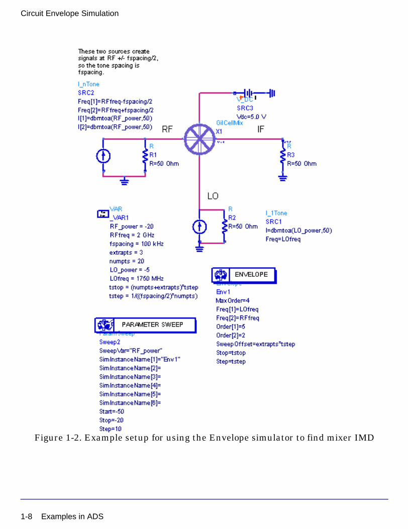
Examples in ADSFigure 1-2 illustrates an example setup for using the Envelope simulator to find mixer intermodulation distortion (IMD).
Note You must have the Circuit Envelope simulator license to simulate examples. You may build the Circuit Envelope example without this license, but will be unable to run the simulations.
Note This design, IMDRFSwpEnv.dsn, is in the Examples directory under RFIC/Mixers_prj. The results are in IMDRFSwpEnv.dds.
Examples in ADS 1-7
Circuit Envelope Simulation
Figure 1-2. Example setup for using the Envelope simulator to find mixer IMD
1-8 Examples in ADS
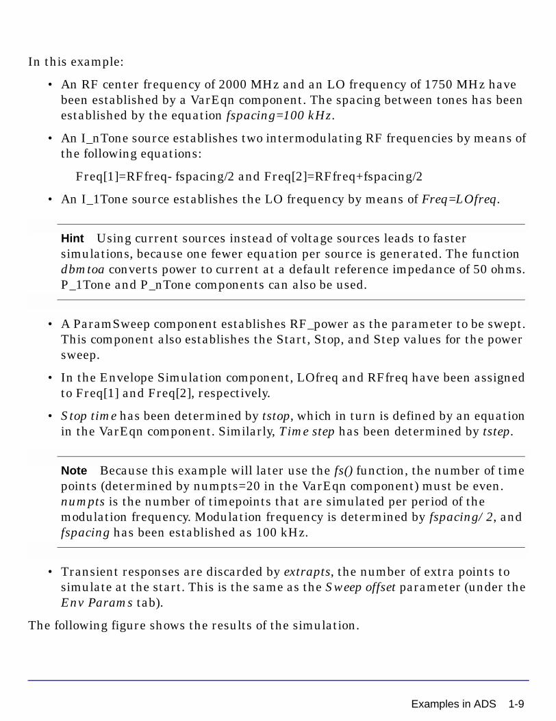
In this example:
• An RF center frequency of 2000 MHz and an LO frequency of 1750 MHz have been established by a VarEqn component. The spacing between tones has been established by the equation fspacing=100 kHz.
• An I_nTone source establishes two intermodulating RF frequencies by means of the following equations:
Freq[1]=RFfreq- fspacing/2 and Freq[2]=RFfreq+fspacing/2
• An I_1Tone source establishes the LO frequency by means of Freq=LOfreq.
Hint Using current sources instead of voltage sources leads to faster simulations, because one fewer equation per source is generated. The function dbmtoa converts power to current at a default reference impedance of 50 ohms. P_1Tone and P_nTone components can also be used.
• A ParamSweep component establishes RF_power as the parameter to be swept. This component also establishes the Start, Stop, and Step values for the power sweep.
• In the Envelope Simulation component, LOfreq and RFfreq have been assigned to Freq[1] and Freq[2], respectively.
• Stop time has been determined by tstop, which in turn is defined by an equation in the VarEqn component. Similarly, Time step has been determined by tstep.
Note Because this example will later use the fs() function, the number of time points (determined by numpts=20 in the VarEqn component) must be even. numpts is the number of timepoints that are simulated per period of the modulation frequency. Modulation frequency is determined by fspacing/2, and fspacing has been established as 100 kHz.
• Transient responses are discarded by extrapts, the number of extra points to simulate at the start. This is the same as the Sweep offset parameter (under the Env Params tab).
The following figure shows the results of the simulation.
Examples in ADS 1-9
Circuit Envelope Simulation
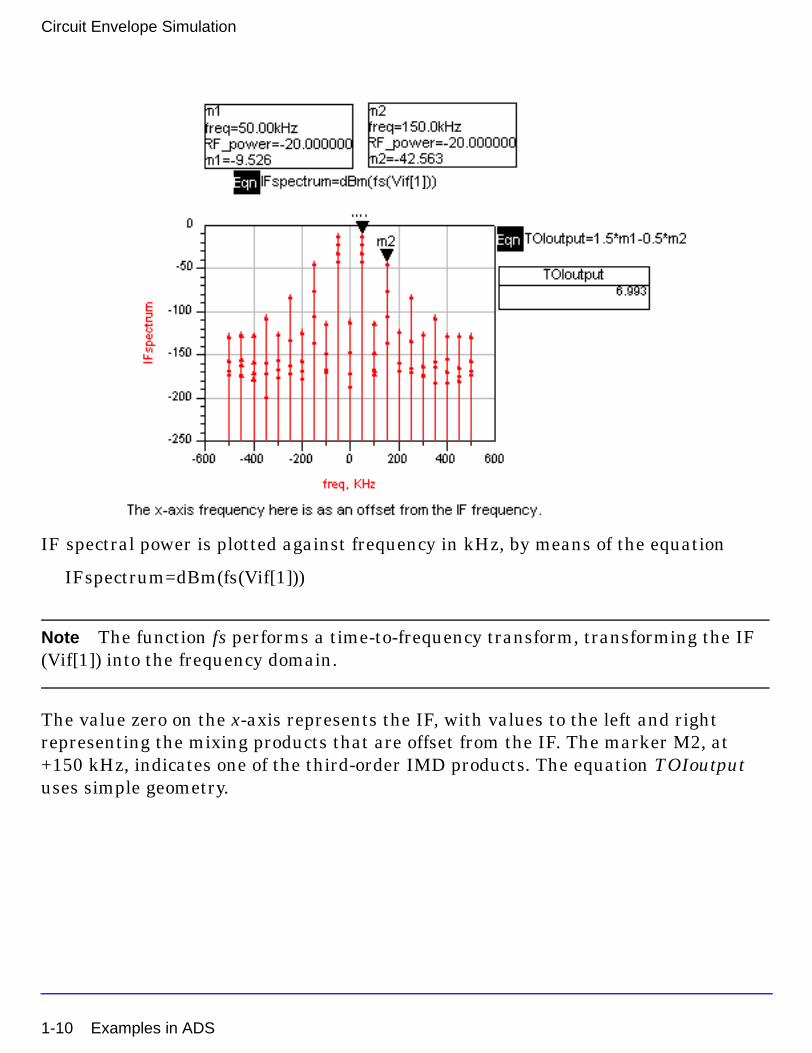
IF spectral power is plotted against frequency in kHz, by means of the equation
IFspectrum=dBm(fs(Vif[1]))
Note The function fs performs a time-to-frequency transform, transforming the IF (Vif[1]) into the frequency domain.
The value zero on the x-axis represents the IF, with values to the left and right representing the mixing products that are offset from the IF. The marker M2, at +150 kHz, indicates one of the third-order IMD products. The equation TOIoutput uses simple geometry.
1-10 Examples in ADS
More Examples
For more Circuit Envelope simulations, refer to these example projects:
• For ways of generating sources for use in envelope simulations (such as π/4–DQPSK, FSK, QAM, and CDMA), see Tutorial/ModSources_prj.
• To simulate amplifier spectral regrowth and adjacent channel power leakage with digitally modulated RF signals at the input, see RF_Board/NADC_PA_prj.
• To simulate PLL transient responses, see RF_Board/PLL_5th_Order_prj and DECT_LO_Synth_prj.
LimitationCircuit Envelope contains the following limitation:
Circuit Envelope assumes that the signal can be expressed in time domain as the product of an envelope and a carrier. In frequency domain, the spectrum of the carrier is a discrete grid of frequency components. The spectrum of the envelope is continuous in a limited bandwidth around each frequency component of the carrier. Normally, Circuit Envelope is more efficient than a broadband Transient when the envelope spectra at adjacent carrier frequency components do not overlap. Otherwise, the broadband Transient or SPICE would be a better alternative. Although there are sporadic cases with overlapping spectra where Circuit Envelope still works better than a Transient, Circuit Envelope is not generally recommended for overlapping spectra. Particularly, when there is an oscillator involved, overlapping spectra might cause convergence problems. Also, envelope noise is not rigorously correct when envelope spectra overlap, because noise in the overlapping spectra is double counted.
Limitation 1-11
Circuit Envelope Simulation
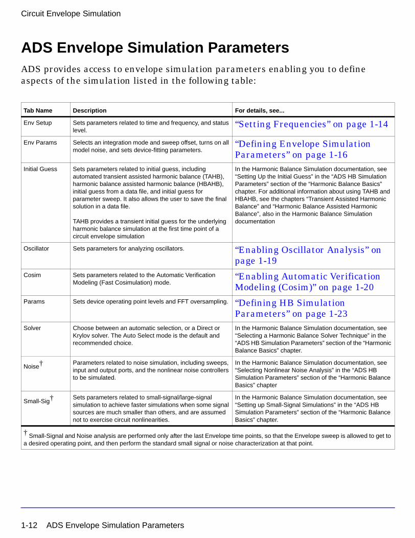
ADS Envelope Simulation ParametersADS provides access to envelope simulation parameters enabling you to define aspects of the simulation listed in the following table:
Tab Name Description For details, see...
Env Setup Sets parameters related to time and frequency, and status level.
“Setting Frequencies” on page 1-14
Env Params Selects an integration mode and sweep offset, turns on all model noise, and sets device-fitting parameters.
“Defining Envelope Simulation Parameters” on page 1-16
Initial Guess Sets parameters related to initial guess, including automated transient assisted harmonic balance (TAHB), harmonic balance assisted harmonic balance (HBAHB), initial guess from a data file, and initial guess for parameter sweep. It also allows the user to save the final solution in a data file.
TAHB provides a transient initial guess for the underlying harmonic balance simulation at the first time point of a circuit envelope simulation
In the Harmonic Balance Simulation documentation, see “Setting Up the Initial Guess” in the “ADS HB Simulation Parameters” section of the “Harmonic Balance Basics” chapter. For additional information about using TAHB and HBAHB, see the chapters “Transient Assisted Harmonic Balance” and “Harmonic Balance Assisted Harmonic Balance”, also in the Harmonic Balance Simulation documentation
Oscillator Sets parameters for analyzing oscillators. “Enabling Oscillator Analysis” on page 1-19
Cosim Sets parameters related to the Automatic Verification Modeling (Fast Cosimulation) mode.
“Enabling Automatic Verification Modeling (Cosim)” on page 1-20
Params Sets device operating point levels and FFT oversampling. “Defining HB Simulation Parameters” on page 1-23
Solver Choose between an automatic selection, or a Direct or Krylov solver. The Auto Select mode is the default and recommended choice.
In the Harmonic Balance Simulation documentation, see “Selecting a Harmonic Balance Solver Technique” in the “ADS HB Simulation Parameters” section of the “Harmonic Balance Basics” chapter.
Noise† Parameters related to noise simulation, including sweeps, input and output ports, and the nonlinear noise controllers to be simulated.
In the Harmonic Balance Simulation documentation, see “Selecting Nonlinear Noise Analysis” in the “ADS HB Simulation Parameters” section of the “Harmonic Balance Basics” chapter
Small-Sig† Sets parameters related to small-signal/large-signal simulation to achieve faster simulations when some signal sources are much smaller than others, and are assumed not to exercise circuit nonlinearities.
In the Harmonic Balance Simulation documentation, see “Setting up Small-Signal Simulations” in the “ADS HB Simulation Parameters” section of the “Harmonic Balance Basics” chapter.
† Small-Signal and Noise analysis are performed only after the last Envelope time points, so that the Envelope sweep is allowed to get to a desired operating point, and then perform the standard small signal or noise characterization at that point.
1-12 ADS Envelope Simulation Parameters
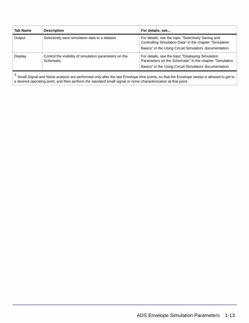
Output Selectively save simulation data to a dataset. For details, see the topic “Selectively Saving and Controlling Simulation Data” in the chapter “Simulation
Basics” in the Using Circuit Simulators documentation
Display Control the visibility of simulation parameters on the Schematic.
For details, see the topic “Displaying Simulation Parameters on the Schematic” in the chapter “Simulation
Basics” in the Using Circuit Simulators documentation
Tab Name Description For details, see...
† Small-Signal and Noise analysis are performed only after the last Envelope time points, so that the Envelope sweep is allowed to get to a desired operating point, and then perform the standard small signal or noise characterization at that point.
ADS Envelope Simulation Parameters 1-13

Circuit Envelope Simulation
Setting Frequencies
The Env Setup tab involves parameters related to time and frequency, and status levels. The following table describes the parameter details. Names listed in the Parameter Name column are used in netlists and on schematics.
Table 1-1. Envelope Simulation Env Setup Parameters
Setup Dialog Name Parameter Name Description
Times
Stop time Stop The time the analysis stops.
Time step Step Sets the fixed time step that the simulator uses to calculate the time-varying envelopes.
Note: The parameter Time step defines the maximum allowed bandwidth (±0.5 /Time step) of the modulation envelope. Because of the nature of the time-domain integration algorithms, the analysis bandwidth (1/Time step) should be at least twice as large as the modulation bandwidth to achieve accurate simulations at the maximum modulation frequencies. Stop time simply defines the maximum duration of the swept time simulation. An analysis starts at time = 0, so the total number of simulation time points that are stored is equal to 1+(Stop time/Time step). At each time point, the envelope values of all of the analysis frequencies, including DC, are saved.
Fundamental Frequencies
Edit Edit the Frequency and Order fields, then use the buttons to Add the frequency to the list displayed under Select.
Frequency Freq[n] The frequency of the fundamental(s). Change by typing over the entry in the field. Select the units (None, Hz, kHz, MHz, GHz) from the drop-down list.
Order Order[n] The maximum order (harmonic number) of the fundamental(s) that will be considered. Change by typing over the entry in the field.
Select Contains the list of fundamental frequencies. Use the Edit field to add fundamental frequencies to this window.
- Add - Enables you to add an item.- Cut - Enables you to delete an item.- Paste - Enables you to take an item that has been cut and place it in a different order.
Maximum mixing order MaxOrder The maximum mixing order of the intermodulation terms in the simulation. The combined order is the sum of the individual frequency orders that are added or subtracted to make up the frequency list. For example, assume there are two fundamentals and Order (see below) is 3.
If Maximum mixing order is 0 or 1, no mixing products are simulated. The frequency list consists of the fundamental and the first, second, and third harmonics of each source.
If Maximum mixing order is 2, the sum and difference frequencies are added to the list.
If Maximum mixing order is 3, the second harmonic of one source can mix with the fundamental of the others, and so on.
1-14 ADS Envelope Simulation Parameters
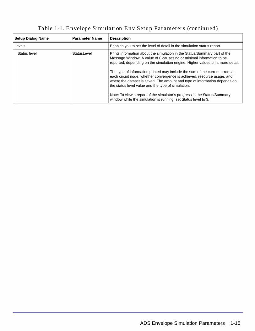
Levels Enables you to set the level of detail in the simulation status report.
Status level StatusLevel Prints information about the simulation in the Status/Summary part of the Message Window. A value of 0 causes no or minimal information to be reported, depending on the simulation engine. Higher values print more detail.
The type of information printed may include the sum of the current errors at each circuit node, whether convergence is achieved, resource usage, and where the dataset is saved. The amount and type of information depends on the status level value and the type of simulation.
Note: To view a report of the simulator’s progress in the Status/Summary window while the simulation is running, set Status level to 3.
Table 1-1. Envelope Simulation Env Setup Parameters (continued)
Setup Dialog Name Parameter Name Description
ADS Envelope Simulation Parameters 1-15
Circuit Envelope Simulation
Defining Envelope Simulation Parameters
The Env Params tab involves selecting an integration mode and sweep offset, turns on all model noise, and sets device-fitting parameters. The following table describes the parameter details. Names listed in the Parameter Name column are used in netlists and on schematics.
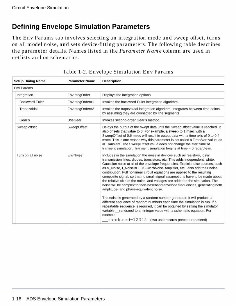
Table 1-2. Envelope Simulation Env Params
Setup Dialog Name Parameter Name Description
Env Params
Integration EnvIntegOrder Displays the integration options.
Backward Euler EnvIntegOrder=1 Invokes the backward-Euler integration algorithm.
Trapezoidal EnvIntegOrder=2 Invokes the trapezoidal integration algorithm. Integrates between time points by assuming they are connected by line segments
Gear’s UseGear Invokes second-order Gear’s method.
Sweep offset SweepOffset Delays the output of the swept data until the SweepOffset value is reached. It also offsets that value to 0. For example, a sweep to 1 msec with a SweepOffset of 0.6 msec will result in output data with a time axis of 0 to 0.4 msec. This is one reason why this parameter is not called a TimeStart value, as in Transient. The SweepOffset value does not change the start time of transient simulation. Transient simulation begins at time = 0 regardless.
Turn on all noise EnvNoise Includes in the simulation the noise in devices such as resistors, lossy transmission lines, diodes, transistors, etc. This adds independent, white, Gaussian noise at all of the envelope frequencies. Explicit noise sources, such as V_Noise, I_NoiseBD, OSCwPhNoise Amplifier, etc., also add their noise contribution. Full nonlinear circuit equations are applied to the resulting composite signal, so that no small-signal assumptions have to be made about the relative size of the noise, and voltages are added to the simulation. The noise will be complex for non-baseband envelope frequencies, generating both amplitude- and phase-equivalent noise.
The noise is generated by a random number generator. It will produce a different sequence of random numbers each time the simulation is run. If a repeatable sequence is required, it can be obtained by setting the simulator variable __randseed to an integer value with a schematic equation. For example,
__randseed=12345 (two underscores precede randseed)
1-16 ADS Envelope Simulation Parameters

Device Fitting There are several ways to control the linear device, time-domain modeling required by the circuit envelope simulator when analyzing a modulation envelope. Most built-in elements now have an Laplace or a transmission line approximation. This parameter is used only with respect to dataset devices or generic linear devices whose frequency response cannot be represented as a rational polynomial of the form
where s is the Laplace variable, T is time delay, and P and Q are the numerator and denominator polynomials, respectively.
For linear elements a model must be generated that reflects the envelope frequency response around each of the analysis frequencies. The first three parameters in this area are used in a pole/zero fit of the frequency response around each carrier frequency. The remaining options are used when a valid or sufficiently accurate pole/zero fit cannot be obtained.
Bandwidth fraction EnvBandwidth Determines what fraction of the envelope bandwidth to use to determine the fit.
The initial value provided for Bandwidth fraction is 1.0. The default value for Bandwidth fraction when the value is left blank is 0.1, so that only the frequency values that lie between ±0.5 x BandwidthFraction/Timestep around each carrier frequency are used to determine the fit.
If greater accuracy is required at the edges of the envelope bandwidth, this number can be increased. However, the simulator will then typically require a higher order and a more time-consuming fit to be generated and then used during the simulation. Also, the integration algorithms cannot maintain 100% percent accuracy out to the edges of the envelope bandwidth.
A Bandwidth fraction value of 0.0 will effectively disable this pole/zero fitting, and just the constant value will be used. This will result in the fastest simulation, but any transient effects from these models will not be included. The Relative tolerance and Absolute tolerance parameters (see below) can also be set to help determine how accurate a fit is desired.
Relative tolerance EnvRelTrunc Sets a relative truncation factor for envelope fitting.
Absolute tolerance EnvAbsTrunc Sets an absolute truncation factor for envelope fitting.
Warn when poor fit EnvWarnPoorFit Causes a warning message to appear when an envelope fit is poor.
Table 1-2. Envelope Simulation Env Params
Setup Dialog Name Parameter Name Description
sT–eP s( )Q s( )------------
ADS Envelope Simulation Parameters 1-17
Circuit Envelope Simulation
Setting Up the Initial Guess
This enables automated transient assisted harmonic balance (TAHB) and harmonic balance assisted harmonic balance (HBAHB). TAHB provides a transient initial guess for the underlying harmonic balance simulation at the first time point of a circuit envelope simulation.
In the Harmonic Balance Simulation documentation, see “Setting Up the Initial Guess” in the “ADS HB Simulation Parameters” section of the “Harmonic Balance Basics” chapter. For additional information about using TAHB and HBAHB, see the chapters “Transient Assisted Harmonic Balance” and “Harmonic Balance Assisted Harmonic Balance”, also in the Harmonic Balance Simulation documentation.
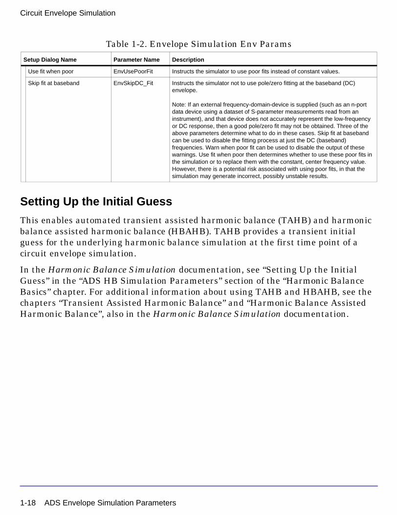
Use fit when poor EnvUsePoorFit Instructs the simulator to use poor fits instead of constant values.
Skip fit at baseband EnvSkipDC_Fit Instructs the simulator not to use pole/zero fitting at the baseband (DC) envelope.
Note: If an external frequency-domain-device is supplied (such as an n-port data device using a dataset of S-parameter measurements read from an instrument), and that device does not accurately represent the low-frequency or DC response, then a good pole/zero fit may not be obtained. Three of the above parameters determine what to do in these cases. Skip fit at baseband can be used to disable the fitting process at just the DC (baseband) frequencies. Warn when poor fit can be used to disable the output of these warnings. Use fit when poor then determines whether to use these poor fits in the simulation or to replace them with the constant, center frequency value. However, there is a potential risk associated with using poor fits, in that the simulation may generate incorrect, possibly unstable results.
Table 1-2. Envelope Simulation Env Params
Setup Dialog Name Parameter Name Description
1-18 ADS Envelope Simulation Parameters
Enabling Oscillator Analysis
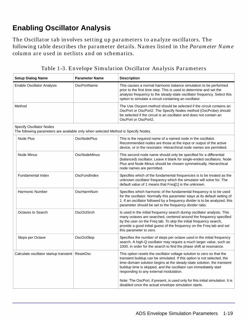
The Oscillator tab involves setting up parameters to analyze oscillators. The following table describes the parameter details. Names listed in the Parameter Name column are used in netlists and on schematics.
Table 1-3. Envelope Simulation Oscillator Analysis Parameters
Setup Dialog Name Parameter Name Description
Enable Oscillator Analysis OscPortName This causes a normal harmonic balance simulation to be performed prior to the first time step. This is used to determine and set the analysis frequency to the steady-state oscillator frequency. Select this option to simulate a circuit containing an oscillator.
Method The Use Oscport method should be selected if the circuit contains an OscPort or OscPort2. The Specify Nodes method (OscProbe) should be selected if the circuit is an oscillator and does not contain an OscPort or OscPort2.
Specify Oscillator NodesThe following parameters are available only when selected Method is Specify Nodes.
Node Plus OscNodePlus This is the required name of a named node in the oscillator. Recommended nodes are those at the input or output of the active device, or in the resonator. Hierarchical node names are permitted.
Node Minus OscNodeMinus This second node name should only be specified for a differential (balanced) oscillator. Leave it blank for single-ended oscillators. Node Plus and Node Minus should be chosen symmetrically. Hierarchical node names are permitted.
Fundamental Index OscFundIndex Specifies which of the fundamental frequencies is to be treated as the unknown oscillator frequency which the simulator will solve for. The default value of 1 means that Freq[1] is the unknown.
Harmonic Number OscHarmNum Specifies which harmonic of the fundamental frequency is to be used for the oscillator. Normally this parameter stays at its default setting of 1. If an oscillator followed by a frequency divider is to be analyzed, this parameter should be set to the frequency divider ratio.
Octaves to Search OscOctSrch Is used in the initial frequency search during oscillator analysis. This many octaves are searched, centered around the frequency specified by the user on the Freq tab. To skip the initial frequency search, provide a good initial guess of the frequency on the Freq tab and set this parameter to zero.
Steps per Octave OscOctStep Specifies the number of steps per octave used in the initial frequency search. A high-Q oscillator may require a much larger value, such as 1000, in order for the search to find the phase shift at resonance.
Calculate oscillator startup transient ResetOsc This option resets the oscillator voltage solution to zero so that the transient buildup can be simulated. If this option is not selected, the time-domain solution begins at the steady-state solution, the transient buildup time is skipped, and the oscillator can immediately start responding to any external modulation.
Note: The OscPort, if present, is used only for this initial simulation. It is disabled once the actual envelope simulation starts.
ADS Envelope Simulation Parameters 1-19

Circuit Envelope Simulation
Enabling Automatic Verification Modeling (Cosim)
These parameters enable and control the Automatic Verification Modeling (Fast Cosimulation) mode and are only applicable when the Envelope controller is being used in a Ptolemy cosimulation. The following table describes the parameter details. Names listed in the Parameter Name column are used in netlists and on schematics.
Table 1-4. Envelope Cosim Parameter and WTB AVM Parameters
Setup Dialog Name Parameter Name Description
Mode
Enable AVM (Fast Cosim) ABM_Mode This enables the Automatic Verification Modeling (Fast Cosimulation) mode to be used for the Analog/RF subcircuit. If AVM (Fast Cosim) is not possible for this subcircuit, then a warning will be output and regular Circuit Envelope Cosimulation will be performed.
Characterization
Max Input Power ABM_MaxPower This specifies the maximum input power to this Analog/RF subcircuit that will be used during the AVM (Fast Cosim) characterization phase. Excessively high values will take longer to characterize due to potentially more difficult circuit convergence. If the input power during the cosimulation exceeds this value, a warning will be generated since the AVM (Fast Cosim) results will no longer be accurate.
Num. of amp. pts. ABM_AmpPts This sets the number of linear amplitude points between 0 and the full scale value defined by the Max Input Power. Depending on how much variation there is in the output vs. input amplitude characterization, more amplitude points may be needed to achieve optimum accuracy at a cost of additional characterization time. Due to the continuation nature of the swept amplitude harmonic balance characterization when not using Krylov modes, the cost of additional amplitude points is usually small. In addition to these linear spaced points, the characterization adds an additional power point every 6 dB down to a value 100 dB below the Max Input Power.
1-20 ADS Envelope Simulation Parameters
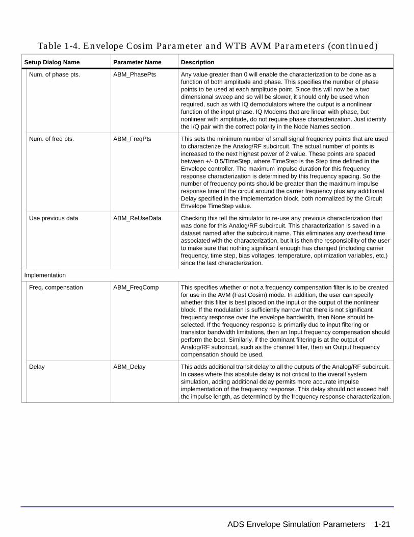
Num. of phase pts. ABM_PhasePts Any value greater than 0 will enable the characterization to be done as a function of both amplitude and phase. This specifies the number of phase points to be used at each amplitude point. Since this will now be a two dimensional sweep and so will be slower, it should only be used when required, such as with IQ demodulators where the output is a nonlinear function of the input phase. IQ Modems that are linear with phase, but nonlinear with amplitude, do not require phase characterization. Just identify the I/Q pair with the correct polarity in the Node Names section.
Num. of freq pts. ABM_FreqPts This sets the minimum number of small signal frequency points that are used to characterize the Analog/RF subcircuit. The actual number of points is increased to the next highest power of 2 value. These points are spaced between +/- 0.5/TimeStep, where TimeStep is the Step time defined in the Envelope controller. The maximum impulse duration for this frequency response characterization is determined by this frequency spacing. So the number of frequency points should be greater than the maximum impulse response time of the circuit around the carrier frequency plus any additional Delay specified in the Implementation block, both normalized by the Circuit Envelope TimeStep value.
Use previous data ABM_ReUseData Checking this tell the simulator to re-use any previous characterization that was done for this Analog/RF subcircuit. This characterization is saved in a dataset named after the subcircuit name. This eliminates any overhead time associated with the characterization, but it is then the responsibility of the user to make sure that nothing significant enough has changed (including carrier frequency, time step, bias voltages, temperature, optimization variables, etc.) since the last characterization.
Implementation
Freq. compensation ABM_FreqComp This specifies whether or not a frequency compensation filter is to be created for use in the AVM (Fast Cosim) mode. In addition, the user can specify whether this filter is best placed on the input or the output of the nonlinear block. If the modulation is sufficiently narrow that there is not significant frequency response over the envelope bandwidth, then None should be selected. If the frequency response is primarily due to input filtering or transistor bandwidth limitations, then an Input frequency compensation should perform the best. Similarly, if the dominant filtering is at the output of Analog/RF subcircuit, such as the channel filter, then an Output frequency compensation should be used.
Delay ABM_Delay This adds additional transit delay to all the outputs of the Analog/RF subcircuit. In cases where this absolute delay is not critical to the overall system simulation, adding additional delay permits more accurate impulse implementation of the frequency response. This delay should not exceed half the impulse length, as determined by the frequency response characterization.
Table 1-4. Envelope Cosim Parameter and WTB AVM Parameters (continued)
Setup Dialog Name Parameter Name Description
ADS Envelope Simulation Parameters 1-21

Circuit Envelope Simulation
Verification
Stop Time ABM_VTime If this verification stop time is not zero, then both the normal Envelope cosimulation and the AVM (Fast Cosim) results are computed. The RMS error between these two results is computed and output after this verification time has ended. This gives an indication as to how well the AVM (Fast Cosim) is matching the Circuit Envelope results.
Accept Tolerance ABM_VTol If the Verification Stop Time has been set, then the resultant RMS error must be less than this value or else the AVM (Fast Cosim) will be turned off and just the normal Envelope cosimulation results will be used for the remainder of the Ptolemy simulation. The stop time must be large enough to account for turn-on delays of filters and to give a sufficiently representative sample of the normal input signal.
Node Names
Active Input ABM_ActiveInputNode When multiple cosimulation inputs exists, only one (or one I/Q pair) can be active. Enter the node name of the active input here. Do not use any node name in the subcircuit input, but use the node name defined at the higher circuit level. If this is an I/Q pair input, then just use either the I or Q node name. Any non-active inputs will be monitored for activity and a warning generated if they are not truly static during a Ptolemy sweep.
IQ Pair ABM_IQ_Nodes[n] If multiple inputs or outputs correspond to an IQ pair, one pair can be defined here. Enter the I node name and the Q node name, as defined in the higher circuit level, separated by a space. If more than one IQ pair exists, use the Other = parameter in the Display tab, and use ABM_IQ_Nodes=”<I node> <Q node>”. Note that for IQ Modems that are linear with respect to phase, phase characterization is not required if the I/Q pair is properly identified here.
Table 1-4. Envelope Cosim Parameter and WTB AVM Parameters (continued)
Setup Dialog Name Parameter Name Description
1-22 ADS Envelope Simulation Parameters
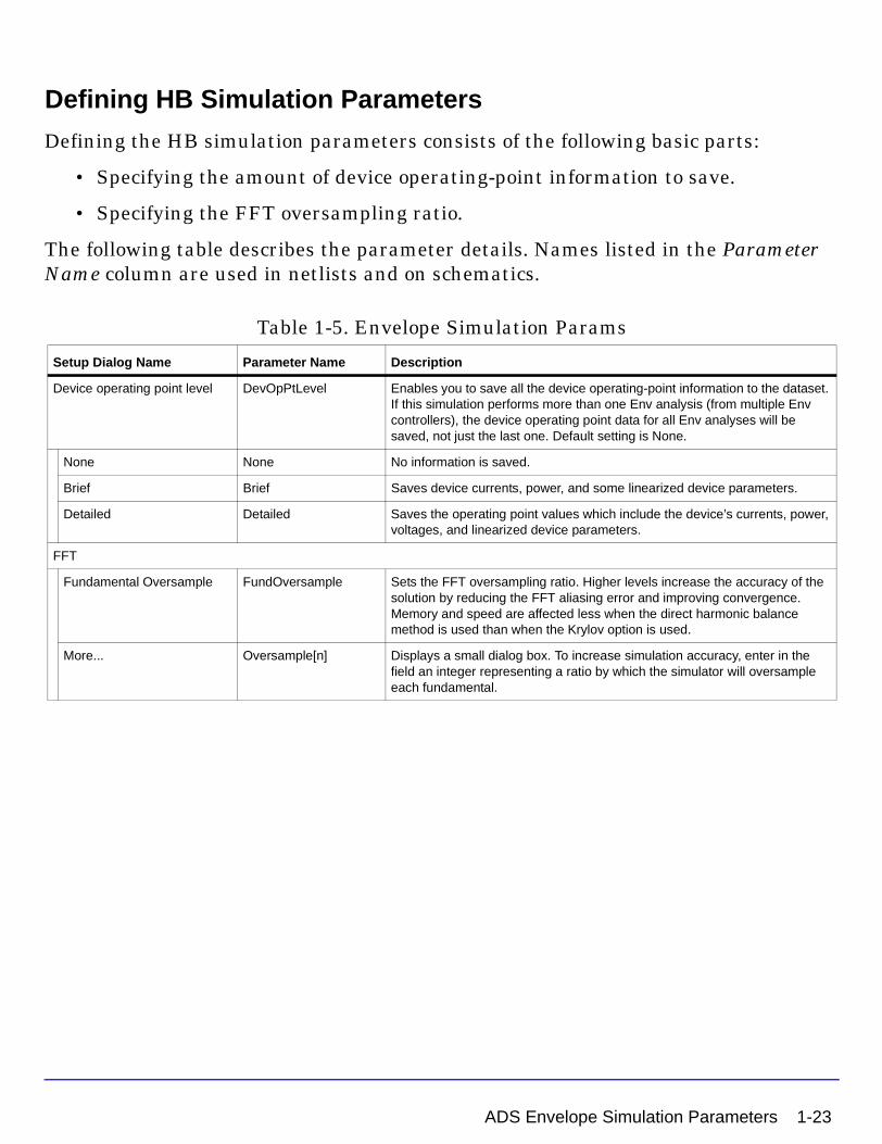
Defining HB Simulation Parameters
Defining the HB simulation parameters consists of the following basic parts:
• Specifying the amount of device operating-point information to save.
• Specifying the FFT oversampling ratio.
The following table describes the parameter details. Names listed in the Parameter Name column are used in netlists and on schematics.
Table 1-5. Envelope Simulation Params
Setup Dialog Name Parameter Name Description
Device operating point level DevOpPtLevel Enables you to save all the device operating-point information to the dataset. If this simulation performs more than one Env analysis (from multiple Env controllers), the device operating point data for all Env analyses will be saved, not just the last one. Default setting is None.
None None No information is saved.
Brief Brief Saves device currents, power, and some linearized device parameters.
Detailed Detailed Saves the operating point values which include the device’s currents, power, voltages, and linearized device parameters.
FFT
Fundamental Oversample FundOversample Sets the FFT oversampling ratio. Higher levels increase the accuracy of the solution by reducing the FFT aliasing error and improving convergence. Memory and speed are affected less when the direct harmonic balance method is used than when the Krylov option is used.
More... Oversample[n] Displays a small dialog box. To increase simulation accuracy, enter in the field an integer representing a ratio by which the simulator will oversample each fundamental.
ADS Envelope Simulation Parameters 1-23
Circuit Envelope Simulation
Selecting a Solver
Use the Solver parameters to select a convergence mode and solver type. These are the same parameters used to set up the solver for harmonic balance simulations. In the Harmonic Balance Simulation documentation, see “Selecting a Harmonic Balance Solver Technique” in the “ADS HB Simulation Parameters” section of the “Harmonic Balance Basics” chapter.
Selecting Noise Analysis
Use the Noise parameters to set up noise analysis including sweeps, input and output ports, and the nonlinear noise controllers to be simulated. These are the same parameters used to set up noise controllers for harmonic balance simulations. In the Harmonic Balance Simulation documentation, see “Selecting Nonlinear Noise Analysis” in the “ADS HB Simulation Parameters” section of the “Harmonic Balance Basics” chapter.
Setting Up Small-Signal Simulations
Use the Small-Signal parameters to use a large-signal/small-signal method to achieve faster simulations when some signal sources are much smaller than others, and are assumed not to exercise circuit nonlinearities.
Small-Signal and Noise analysis are performed only after the last Envelope time points, so that the Envelope sweep is allowed to get to a desired operating point, and then perform the standard small signal or noise characterization at that point.
These are the same parameters used to set up small-signal simulations for harmonic balance. In the Harmonic Balance Simulation documentation, see “Setting up Small-Signal Simulations” in the “ADS HB Simulation Parameters” section of the “Harmonic Balance Basics” chapter.
1-24 ADS Envelope Simulation Parameters

RFDE Envelope Analysis ParametersRFDE provides access to circuit envelope analysis parameters enabling you to define aspects of the simulation listed in the following table:
Parameter Group Description For details, see...
Time Setup Sets parameters related to stop time and time step for the analysis.
“Setting Up Time Parameters” on page 1-26
Fundamental Tones
Sets the fundamental frequency and order, and the FFT oversample ratio.
“Setting Up Fundamental Tones” on page 1-27
Annotation Status level and device operating point level. “Setting Up the Annotation” on page 1-28
Initial Guess Sets parameters related to initial guess, including automated transient assisted harmonic balance (TAHB), harmonic balance assisted harmonic balance (HBAHB), initial guess from a data file, and initial guess for parameter sweep. It also allows the user to save the final solution in a data file. For details, see the chapter “Harmonic Balance Basics” in the Harmonic Balance Simulation documentation.
“Setting Up the Initial Guess” on page 1-29
Oscillator Sets parameters for analyzing oscillators. “Enabling Oscillator Simulation” on page 1-32
Nonlinear Noise Parameters related to noise simulation, including sweeps, and input/output ports to be simulated.
“Setting Up Nonlinear Noise Parameters” on page 1-33
Small Signal Simulation
Sets parameters related to small-signal/large-signal simulation.
“Setting Up Small-Signal Simulations” on page 1-38
Convergence / Solver
Choose between an automatic selection, or a Direct or Krylov solver. The Auto Select mode is the default and recommended choice. For information about choosing solvers, see the chapter “Harmonic Balance Basics” in the Harmonic Balance Simulation documentation.
“Selecting a Harmonic Balance Convergence/Solver Technique” on page 1-40
Other Enables access to hidden parameters, typically for troubleshooting.
“Defining Other Parameters” on page 1-48
RFDE Envelope Analysis Parameters 1-25
Circuit Envelope Simulation
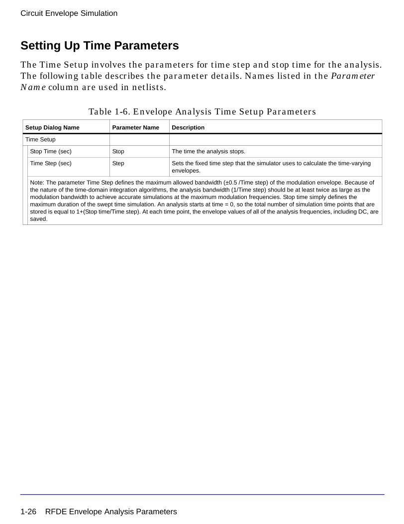
Setting Up Time Parameters
The Time Setup involves the parameters for time step and stop time for the analysis. The following table describes the parameter details. Names listed in the Parameter Name column are used in netlists.
Table 1-6. Envelope Analysis Time Setup Parameters
Setup Dialog Name Parameter Name Description
Time Setup
Stop Time (sec) Stop The time the analysis stops.
Time Step (sec) Step Sets the fixed time step that the simulator uses to calculate the time-varying envelopes.
Note: The parameter Time Step defines the maximum allowed bandwidth (±0.5 /Time step) of the modulation envelope. Because of the nature of the time-domain integration algorithms, the analysis bandwidth (1/Time step) should be at least twice as large as the modulation bandwidth to achieve accurate simulations at the maximum modulation frequencies. Stop time simply defines the maximum duration of the swept time simulation. An analysis starts at time = 0, so the total number of simulation time points that are stored is equal to 1+(Stop time/Time step). At each time point, the envelope values of all of the analysis frequencies, including DC, are saved.
1-26 RFDE Envelope Analysis Parameters
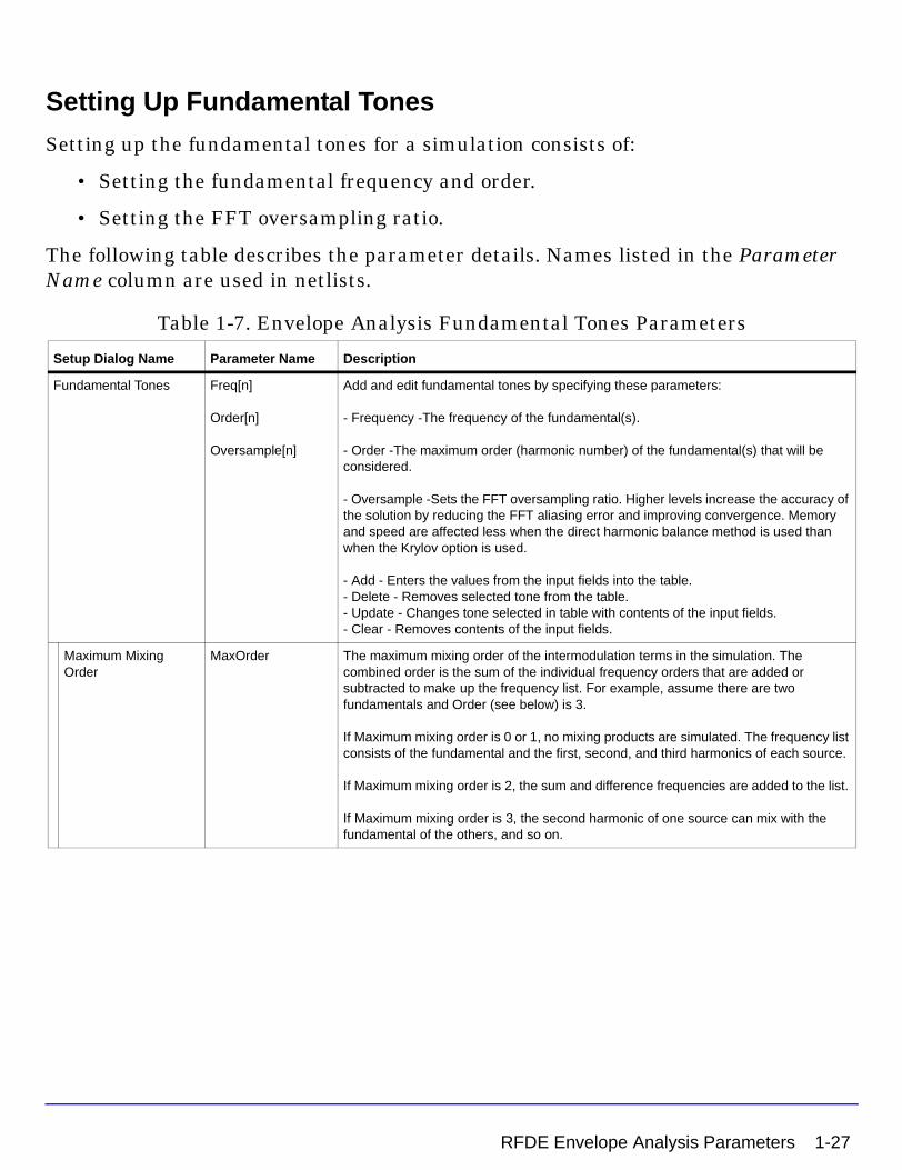
Setting Up Fundamental Tones
Setting up the fundamental tones for a simulation consists of:
• Setting the fundamental frequency and order.
• Setting the FFT oversampling ratio.
The following table describes the parameter details. Names listed in the Parameter Name column are used in netlists.
Table 1-7. Envelope Analysis Fundamental Tones Parameters
Setup Dialog Name Parameter Name Description
Fundamental Tones Freq[n]
Order[n]
Oversample[n]
Add and edit fundamental tones by specifying these parameters:
- Frequency -The frequency of the fundamental(s).
- Order -The maximum order (harmonic number) of the fundamental(s) that will be considered.
- Oversample -Sets the FFT oversampling ratio. Higher levels increase the accuracy of the solution by reducing the FFT aliasing error and improving convergence. Memory and speed are affected less when the direct harmonic balance method is used than when the Krylov option is used.
- Add - Enters the values from the input fields into the table.- Delete - Removes selected tone from the table.- Update - Changes tone selected in table with contents of the input fields.- Clear - Removes contents of the input fields.
Maximum Mixing Order
MaxOrder The maximum mixing order of the intermodulation terms in the simulation. The combined order is the sum of the individual frequency orders that are added or subtracted to make up the frequency list. For example, assume there are two fundamentals and Order (see below) is 3.
If Maximum mixing order is 0 or 1, no mixing products are simulated. The frequency list consists of the fundamental and the first, second, and third harmonics of each source.
If Maximum mixing order is 2, the sum and difference frequencies are added to the list.
If Maximum mixing order is 3, the second harmonic of one source can mix with the fundamental of the others, and so on.
RFDE Envelope Analysis Parameters 1-27

Circuit Envelope Simulation
Setting Up the Annotation
Setting up the annotation for a simulation consists of:
• Setting the Status Level.
• Setting the Device Operating Point Level.
The following table describes the parameter details. Names listed in the Parameter Name column are used in netlists.
Table 1-8. Envelope Analysis Annotation Parameters
Setup Dialog Name Parameter Name Description
Annotation Enables you to set the level of detail in the simulation status report.
Status Level StatusLevel Prints information about the simulation in the Status/Summary part of the Message Window.- 0 reports little or no information, depending on the simulation engine.- 1 and 2 yield more detail.- Use 3 and 4 sparingly since they increase process size and simulation times considerably.
The type of information printed may include the sum of the current errors at each circuit node, whether convergence is achieved, resource usage, and where the dataset is saved. The amount and type of information depends on the status level value and the type of simulation.
Note: To view a report of the simulator’s progress in the Status/Summary window while the simulation is running, set Status level to 3.
Device Operating Point Level
DevOpPtLevel Enables you to save all the device operating-point information to the dataset. Default setting is None.
None None No information is saved.
Brief Brief Saves device currents, power, and some linearized device parameters.
Detailed Detailed Saves the operating point values which include the device’s currents, power, voltages, and linearized device parameters.
1-28 RFDE Envelope Analysis Parameters

Setting Up the Initial Guess
Setting up the initial guess for a harmonic balance simulation consists of:
• Setting Transient Assisted Harmonic Balance (TAHB).
• Setting Harmonic Balance Assisted Harmonic Balance (HBAHB).
• Setting Initial Guess and Final Solution parameters.
TAHB provides a transient initial guess for the underlying harmonic balance simulation at the first time point of a circuit envelope simulation.
To set up a TAHB analysis:
• Select Envelope analysis. In the setup dialog box, click Options. In the Circuit Envelope Options dialog box, scroll to TAHB and select Auto, On, or Off for TAHB.
It is recommended to use the TAHB Auto mode, which is the default setting, for optimal performance. The simulator will turn on TAHB automatically if the circuit involves a divider. The TAHB On and Off modes are for you to manually turn on or off TAHB, which should only be used when you would like to override the simulator's automatic choice.
By enabling TAHB, the simulator will generate its own transient initial guess for Envelope analysis. You do not need to supply an initial guess. TAHB is required whenever the circuit contains a frequency divider.
To set up a HBAHB analysis:
• In the Circuit Envelope Options dialog box, in the section Harmonic Balance Assisted Harmonic Balance, select either Auto, On, or Off.
The Auto mode is the default and is recommended, which allows the simulator to determine whether to use HBAHB and to optimize the HBAHB setup if it is used. Selecting the On mode forces HBAHB to be turned on and the default sequencing (1-tone, 2-tone, ...) will be used. Selecting the Off mode forces HBAHB to be turned off.
By using HBAHB, the simulator will generate its own initial guess for multi-tone Harmonic Balance from another harmonic balance analysis with fewer fundamental frequencies than the original multi-tone problem. You do not need to supply an initial guess. If you do provide an initial guess by enabling Use Initial Guess and entering a name for File (parameters UseInFile and InFile), then that will take precedence over HBAHB so long as the file exists. For additional information about using TAHB and
RFDE Envelope Analysis Parameters 1-29

Circuit Envelope Simulation
HBAHB, see “Transient Assisted Harmonic Balance” and “Harmonic Balance Assisted Harmonic Balance”, in the Harmonic Balance Simulation documentation.
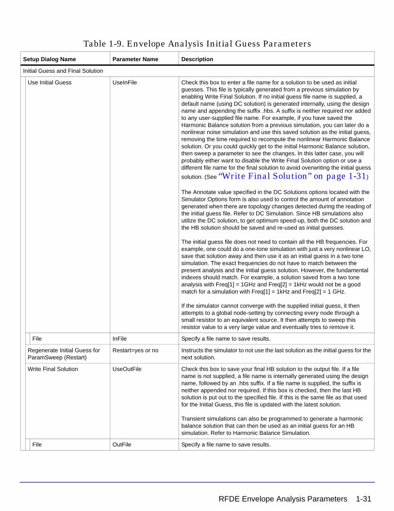
The following table shows the parameters available to set TAHB, HBAHB, and Initial Guess. Names listed in the Parameter Name column are used in netlists.
Table 1-9. Envelope Analysis Initial Guess Parameters
Setup Dialog Name Parameter Name Description
Transient Assisted Harmonic Balance
TAHB_Enable Set the TAHB mode to Auto (default), On, or Off. Auto is set automatically if the circuit contains a divider. Choose On or Off to override the default settings. The Advanced Transient Settings are available when On is set.
Transient Setup
Transient StopTime StopTime This is the transient stop time. The default is 100 cycles of the commensurate frequency. The commensurate frequency for a single tone simulation will be Freq[1]. If steady state is detected earlier than the StopTime, then transient will end earlier than the StopTime.
Transient MaxTimeStep MaxTimeStep This is the transient maximum time step. The default is 1/(8 x Maximum frequency).
Additional Transient Parameters
Min Detect Steady State Time SteadyStateMinTime This is the earliest point in time that the transient simulator starts checking for steady state conditions. If your circuit exhibits a large amount of over/undershoot, then this needs to be larger than the default so that the detector will begin to check for steady state after some of the initial transients have settled
Transient IV_RelTol IV_RelTol This is the transient relative voltage and current tolerance. The default is 1e-3. When simulation options are included in the simulation (using Simulation > Options in RFDE’s Analog Design Environment window), use this value to set specific relative tolerances to be used for transient only. The value will be used for both current and voltage relative tolerance for transient.
Transient Other Enables ability to set other transient simulation parameters that are not found in this dialog box. For example, use this parameter to set the following transient convolution parameter ImpMaxFreq=10 GHz.
Use only Freq[1] for transient Tells the simulator to perform a single tone transient simulation for a multitone harmonic balance simulation. The default setting is enabled.
Output Transient Data to Dataset
SaveToDataset When enabled, the transient simulation data used in generating the initial guess is output to the dataset, in addition to the final harmonic balance data. For large circuits, this can cause the datasets to become quite large.
Harmonic Balance Assisted Harmonic Balance
HBAHB_Enable Set the HBAHB mode to Auto, On, or Off.
1-30 RFDE Envelope Analysis Parameters
Initial Guess and Final Solution
Use Initial Guess UseInFile Check this box to enter a file name for a solution to be used as initial guesses. This file is typically generated from a previous simulation by enabling Write Final Solution. If no initial guess file name is supplied, a default name (using DC solution) is generated internally, using the design name and appending the suffix .hbs. A suffix is neither required nor added to any user-supplied file name. For example, if you have saved the Harmonic Balance solution from a previous simulation, you can later do a nonlinear noise simulation and use this saved solution as the initial guess, removing the time required to recompute the nonlinear Harmonic Balance solution. Or you could quickly get to the initial Harmonic Balance solution, then sweep a parameter to see the changes. In this latter case, you will probably either want to disable the Write Final Solution option or use a different file name for the final solution to avoid overwriting the initial guess
solution. (See “Write Final Solution” on page 1-31)
The Annotate value specified in the DC Solutions options located with the Simulator Options form is also used to control the amount of annotation generated when there are topology changes detected during the reading of the initial guess file. Refer to DC Simulation. Since HB simulations also utilize the DC solution, to get optimum speed-up, both the DC solution and the HB solution should be saved and re-used as initial guesses.
The initial guess file does not need to contain all the HB frequencies. For example, one could do a one-tone simulation with just a very nonlinear LO, save that solution away and then use it as an initial guess in a two tone simulation. The exact frequencies do not have to match between the present analysis and the initial guess solution. However, the fundamental indexes should match. For example, a solution saved from a two tone analysis with Freq[1] = 1GHz and Freq[2] = 1kHz would not be a good match for a simulation with Freq[1] = 1kHz and Freq[2] = 1 GHz.
If the simulator cannot converge with the supplied initial guess, it then attempts to a global node-setting by connecting every node through a small resistor to an equivalent source. It then attempts to sweep this resistor value to a very large value and eventually tries to remove it.
File InFile Specify a file name to save results.
Regenerate Initial Guess for ParamSweep (Restart)
Restart=yes or no Instructs the simulator to not use the last solution as the initial guess for the next solution.
Write Final Solution UseOutFile Check this box to save your final HB solution to the output file. If a file name is not supplied, a file name is internally generated using the design name, followed by an .hbs suffix. If a file name is supplied, the suffix is neither appended nor required. If this box is checked, then the last HB solution is put out to the specified file. If this is the same file as that used for the Initial Guess, this file is updated with the latest solution.
Transient simulations can also be programmed to generate a harmonic balance solution that can then be used as an initial guess for an HB simulation. Refer to Harmonic Balance Simulation.
File OutFile Specify a file name to save results.
Table 1-9. Envelope Analysis Initial Guess Parameters
Setup Dialog Name Parameter Name Description
RFDE Envelope Analysis Parameters 1-31

Circuit Envelope Simulation
Enabling Oscillator Simulation
To set up oscillator simulation, select the Oscillator option, then set the oscillator parameters. The following table describes the parameter details. Names listed in the Parameter Name column are used in netlists.
Table 1-10. Envelope Analysis Oscillator Simulation Parameters
Setup Dialog Name Parameter Name Description
Oscillator OscPortName This causes a normal harmonic balance simulation to be performed prior to the first time step. This is used to determine and set the analysis frequency to the steady-state oscillator frequency. Select this option to simulate a circuit containing an oscillator.
Method =yes (Oscport)
=<name> (OscProbe)
The Use Oscport method should be selected if the circuit contains an OscPort or OscPort2. The Specify Oscillator Nodes method (OscProbe) should be selected if the circuit is an oscillator and does not contain an OscPort or OscPort2.
Specify Oscillator Nodes (OscProbe)The following parameters are available only when selected Method is Specify Oscillator Nodes.
Node Plus Node[1] This is the required name of a named node in the oscillator. Recommended nodes are those at the input or output of the active device, or in the resonator. Hierarchical node names are permitted.
Node Minus Node[2] This second node name should only be specified for a differential (balanced) oscillator. Leave it blank for single-ended oscillators. Node Plus and Node Minus should be chosen symmetrically. Hierarchical node names are permitted.
Fundamental Index FundIndex Specifies which of the fundamental frequencies is to be treated as the unknown oscillator frequency which the simulator will solve for. The default value of 1 means that Freq[1] is the unknown.
Harmonic Number Harm Specifies which harmonic of the fundamental frequency is to be used for the oscillator. Normally this parameter stays at its default setting of 1. If an oscillator followed by a frequency divider is to be analyzed, this parameter should be set to the frequency divider ratio.
Octaves to Search NumOctaves Is used in the initial frequency search during oscillator analysis. This many octaves are searched, centered around the frequency specified by the user for the Time Setup parameters. To skip the initial frequency search, provide a good initial guess of the frequency for Time Setup and set this parameter to zero.
Steps per Octave Steps Specifies the number of steps per octave used in the initial frequency search. A high-Q oscillator may require a much larger value, such as 1000, in order for the search to find the phase shift at resonance.
Calculate Oscillator Startup Transient
ResetOsc This option resets the oscillator voltage solution to zero so that the transient buildup can be simulated. If this option is not selected, the time-domain solution begins at the steady-state solution, the transient buildup time is skipped, and the oscillator can immediately start responding to any external modulation.
Note: The OscPort, if present, is used only for this initial simulation. It is disabled once the actual envelope simulation starts.
1-32 RFDE Envelope Analysis Parameters

Setting Up Nonlinear Noise Parameters
Defining the noise parameters consists of the following basic parts:
• Enabling the noise option to request a noise analysis and edit parameters.
• Specifying the noise type, nodes, and frequency (or sweep plan).
• Specifying the noise nodes to use for noise parameter calculation.
• Specifying the noise contributors and the threshold for noise contribution.
• Specifying the bandwidth over which the noise simulation is performed.
The following table describes the parameter details.
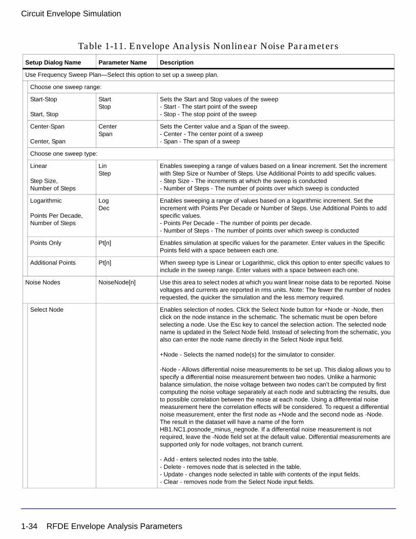
Table 1-11. Envelope Analysis Nonlinear Noise Parameters
Setup Dialog Name Parameter Name Description
Nonlinear Noise NoiseCon Enables nonlinear noise analysis.
Noise Type
Noise Voltage and/or Noise Figure
PhaseNoise=0 A standard noise simulation where noise voltages and/or noise figure are computed at the requested nodes at specified noise frequencies.
Phase Noise PhaseNoise=1 Specifies that a phase noise simulation should be performed instead of a standard noise simulation. Phase noise can be simulated for any type of circuit, not just an oscillator. For example, this makes it possible to simulate the added phase noise due to an amplifier. Phase noise can also be computed around any large signal carrier frequency, not just the fundamental frequency of an oscillator. This makes it possible to simulate the phase noise after an oscillator signal passes through a frequency multiplier or mixer.
Noise FrequencyorOffset Frequency
FreqForNoise The parameter name changes with the Noise Type setting. For either parameter, enter a value for a single frequency point or set up a frequency sweep plan to sweep frequencies.
Noise Frequency - Sets the frequency at which the noise is computed.
Offset Frequency - Sets the offset frequency from a large signal carrier which is specified in the Carrier Frequency section below. Noise simulation is performed at the specified frequencies.
RFDE Envelope Analysis Parameters 1-33
Circuit Envelope Simulation
Use Frequency Sweep Plan—Select this option to set up a sweep plan.
Choose one sweep range:
Start-Stop
Start, Stop
StartStop
Sets the Start and Stop values of the sweep- Start - The start point of the sweep- Stop - The stop point of the sweep
Center-Span
Center, Span
CenterSpan
Sets the Center value and a Span of the sweep.- Center - The center point of a sweep- Span - The span of a sweep
Choose one sweep type:
Linear
Step Size, Number of Steps
LinStep
Enables sweeping a range of values based on a linear increment. Set the increment with Step Size or Number of Steps. Use Additional Points to add specific values.- Step Size - The increments at which the sweep is conducted- Number of Steps - The number of points over which sweep is conducted
Logarithmic
Points Per Decade, Number of Steps
LogDec
Enables sweeping a range of values based on a logarithmic increment. Set the increment with Points Per Decade or Number of Steps. Use Additional Points to add specific values.- Points Per Decade - The number of points per decade.- Number of Steps - The number of points over which sweep is conducted
Points Only Pt[n] Enables simulation at specific values for the parameter. Enter values in the Specific Points field with a space between each one.
Additional Points Pt[n] When sweep type is Linear or Logarithmic, click this option to enter specific values to include in the sweep range. Enter values with a space between each one.
Noise Nodes NoiseNode[n] Use this area to select nodes at which you want linear noise data to be reported. Noise voltages and currents are reported in rms units. Note: The fewer the number of nodes requested, the quicker the simulation and the less memory required.
Select Node Enables selection of nodes. Click the Select Node button for +Node or -Node, then click on the node instance in the schematic. The schematic must be open before selecting a node. Use the Esc key to cancel the selection action. The selected node name is updated in the Select Node field. Instead of selecting from the schematic, you also can enter the node name directly in the Select Node input field.
+Node - Selects the named node(s) for the simulator to consider.
-Node - Allows differential noise measurements to be set up. This dialog allows you to specify a differential noise measurement between two nodes. Unlike a harmonic balance simulation, the noise voltage between two nodes can’t be computed by first computing the noise voltage separately at each node and subtracting the results, due to possible correlation between the noise at each node. Using a differential noise measurement here the correlation effects will be considered. To request a differential noise measurement, enter the first node as +Node and the second node as -Node. The result in the dataset will have a name of the form HB1.NC1.posnode_minus_negnode. If a differential noise measurement is not required, leave the -Node field set at the default value. Differential measurements are supported only for node voltages, not branch current.
- Add - enters selected nodes into the table.- Delete - removes node that is selected in the table.- Update - changes node selected in table with contents of the input fields.- Clear - removes node from the Select Node input fields.
Table 1-11. Envelope Analysis Nonlinear Noise Parameters
Setup Dialog Name Parameter Name Description
1-34 RFDE Envelope Analysis Parameters

Compute Noise Figure—This option is available when Noise Type is Noise Voltage and/or Noise Figure.
Input Frequency InputFreq Because the simulator uses a single-sideband definition of noise figure, the correct input sideband frequency must be specified here. This parameter identifies which input frequency will mix to the noise frequency of interest.
In the case of mixers, Input frequency is typically determined by an equation that involves the local oscillator (LO) frequency and the noise frequency. Either the sum of or difference between these two values is used, depending on whether upconversion or downconversion is taking place.
The above parameters do not need to be specified if only the output noise voltage is desired (that is, if no noise figure is computed).
Input Port Number NoiseInputPort Number of the source port at which noise is injected. This is commonly the RF port. Although any valid port number can be used, the input port number is frequently defined as 1. Use the Select button to select the input port from the schematic, or enter the port number directly in the input field.
Output Port Number NoiseOutputPort Number of the Term component at which noise is retrieved. This is commonly the IF port. Although any valid port number can be used, the output port number is frequently defined as 2. Use the Select button to select the output port from the schematic, or enter the port number directly in the input field.
Carrier Frequency—This option is available when Noise Type is Phase Noise.
Specification Method The frequency of the large signal carrier used in all but the normal noise simulation are specified within this group of parameters. Any large signal carrier from the harmonic balance simulation may serve as the carrier frequency for phase noise simulation. There are two ways to specify the carrier frequency:
Select Carrier Mixing Indices, then enter the indices.orSelect Carrier Frequency, then enter the frequency.
Carrier Mixing Indices Select this method, then specify the indices in the Index List entry field.
Carrier Frequency Select this method, then specify the frequency in the Frequency entry field.
Index List CarrierIndex[n] When the Specification Method is Carrier Mixing Indices, enter values for the Index List. For example, the lower sideband mixing term in a mixer would be entered as 1 and -1. The indices are listed in sequential order by carrier.
Frequency CarrierFreq When the Specification Method is Carrier Frequency, enter a value for Frequency. Enter either a number or a variable name. Since the frequency may not be precisely known in an oscillator, the simulator searches for the frequency closest to the user-specified frequency. If the difference between the user-specified frequency and the actual large-signal frequency exceeds 10%, a warning message will be issued. A carrier frequency of zero cannot be entered directly as zero due to a limitation in the simulator; enter a small value such as 1 Hz instead.
Table 1-11. Envelope Analysis Nonlinear Noise Parameters
Setup Dialog Name Parameter Name Description
RFDE Envelope Analysis Parameters 1-35
Circuit Envelope Simulation
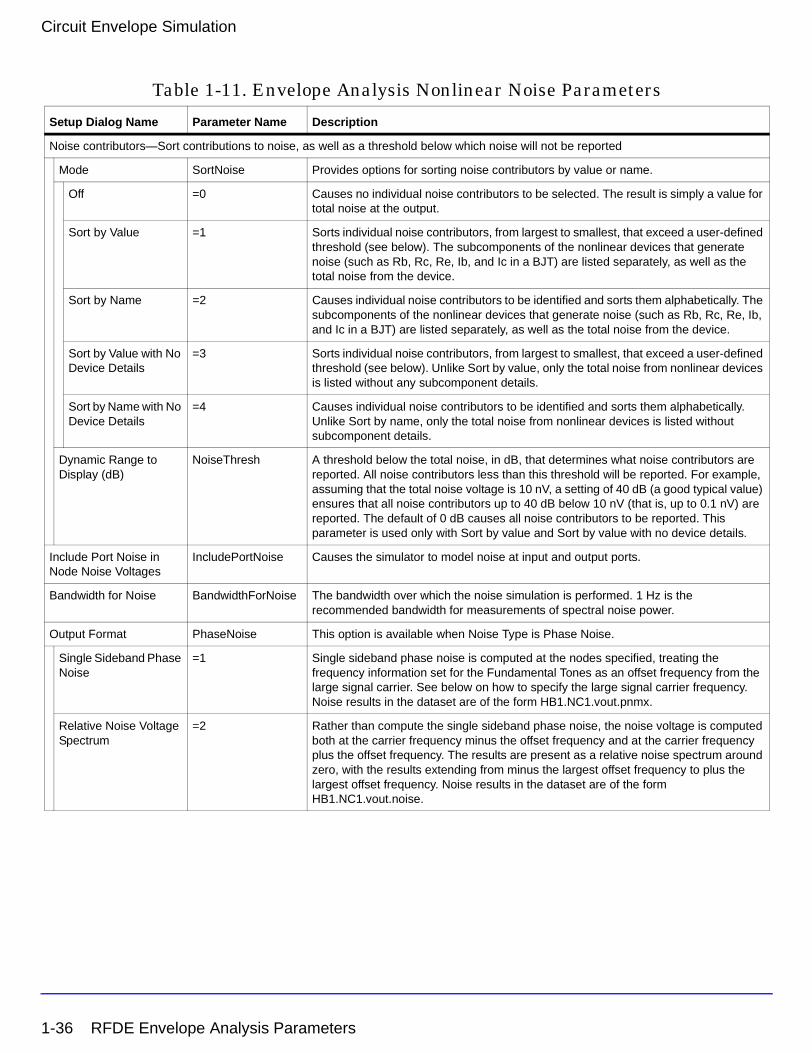
Noise contributors—Sort contributions to noise, as well as a threshold below which noise will not be reported
Mode SortNoise Provides options for sorting noise contributors by value or name.
Off =0 Causes no individual noise contributors to be selected. The result is simply a value for total noise at the output.
Sort by Value =1 Sorts individual noise contributors, from largest to smallest, that exceed a user-defined threshold (see below). The subcomponents of the nonlinear devices that generate noise (such as Rb, Rc, Re, Ib, and Ic in a BJT) are listed separately, as well as the total noise from the device.
Sort by Name =2 Causes individual noise contributors to be identified and sorts them alphabetically. The subcomponents of the nonlinear devices that generate noise (such as Rb, Rc, Re, Ib, and Ic in a BJT) are listed separately, as well as the total noise from the device.
Sort by Value with No Device Details
=3 Sorts individual noise contributors, from largest to smallest, that exceed a user-defined threshold (see below). Unlike Sort by value, only the total noise from nonlinear devices is listed without any subcomponent details.
Sort by Name with No Device Details
=4 Causes individual noise contributors to be identified and sorts them alphabetically. Unlike Sort by name, only the total noise from nonlinear devices is listed without subcomponent details.
Dynamic Range to Display (dB)
NoiseThresh A threshold below the total noise, in dB, that determines what noise contributors are reported. All noise contributors less than this threshold will be reported. For example, assuming that the total noise voltage is 10 nV, a setting of 40 dB (a good typical value) ensures that all noise contributors up to 40 dB below 10 nV (that is, up to 0.1 nV) are reported. The default of 0 dB causes all noise contributors to be reported. This parameter is used only with Sort by value and Sort by value with no device details.
Include Port Noise in Node Noise Voltages
IncludePortNoise Causes the simulator to model noise at input and output ports.
Bandwidth for Noise BandwidthForNoise The bandwidth over which the noise simulation is performed. 1 Hz is the recommended bandwidth for measurements of spectral noise power.
Output Format PhaseNoise This option is available when Noise Type is Phase Noise.
Single Sideband Phase Noise
=1 Single sideband phase noise is computed at the nodes specified, treating the frequency information set for the Fundamental Tones as an offset frequency from the large signal carrier. See below on how to specify the large signal carrier frequency. Noise results in the dataset are of the form HB1.NC1.vout.pnmx.
Relative Noise Voltage Spectrum
=2 Rather than compute the single sideband phase noise, the noise voltage is computed both at the carrier frequency minus the offset frequency and at the carrier frequency plus the offset frequency. The results are present as a relative noise spectrum around zero, with the results extending from minus the largest offset frequency to plus the largest offset frequency. Noise results in the dataset are of the form HB1.NC1.vout.noise.
Table 1-11. Envelope Analysis Nonlinear Noise Parameters
Setup Dialog Name Parameter Name Description
1-36 RFDE Envelope Analysis Parameters
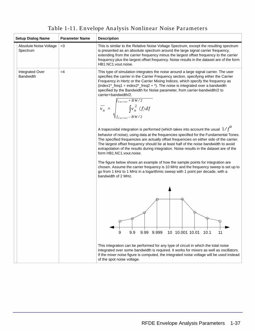
Absolute Noise Voltage Spectrum
=3 This is similar to the Relative Noise Voltage Spectrum, except the resulting spectrum is presented as an absolute spectrum around the large signal carrier frequency, extending from the carrier frequency minus the largest offset frequency to the carrier frequency plus the largest offset frequency. Noise results in the dataset are of the form HB1.NC1.vout.noise.
Integrated Over Bandwidth
=4 This type of simulation integrates the noise around a large signal carrier. The user specifies the carrier in the Carrier Frequency section, specifying either the Carrier Frequency in Hertz or the Carrier Mixing Indices, which specify the frequency as (index1*_freq1 + index2*_freq2 + *). The noise is integrated over a bandwidth specified by the Bandwidth for Noise parameter, from carrier-bandwidth/2 to carrier+bandwidth/2.
A trapezoidal integration is performed (which takes into account the usual behavior of noise), using data at the frequencies specified for the Fundamental Tones. The specified frequencies are actually offset frequencies on either side of the carrier. The largest offset frequency should be at least half of the noise bandwidth to avoid extrapolation of the results during integration. Noise results in the dataset are of the form HB1.NC1.vout.noise.
The figure below shows an example of how the sample points for integration are chosen. Assume the carrier frequency is 10 MHz and the frequency sweep is set up to go from 1 kHz to 1 MHz in a logarithmic sweep with 1 point per decade, with a bandwidth of 2 MHz.
This integration can be performed for any type of circuit in which the total noise integrated over some bandwidth is required. It works for mixers as well as oscillators. If the mixer noise figure is computed, the integrated noise voltage will be used instead of the spot noise voltage.
Table 1-11. Envelope Analysis Nonlinear Noise Parameters
Setup Dialog Name Parameter Name Description
vn vn2 f⟨ ⟩ fd
fCarrier BW 2⁄–
fCarrier BW 2⁄+
∫=
1 fα⁄
9 9.9 9.99 9.999 10 10.001 10.01 10.1 11
RFDE Envelope Analysis Parameters 1-37

Circuit Envelope Simulation
Setting Up Small-Signal Simulations
Defining the small-signal simulation parameters consists of the following basic parts:
• Enabling the option to request a small-signal analysis and edit parameters.
• Specifying the frequency (or sweep plan).
• Specifying options to use of all small-signal frequencies and merge with large-signal frequencies.
This feature uses a large-signal/small-signal method to achieve faster simulations when some signal sources are much smaller than others, and can be assumed not to exercise circuit nonlinearities. For example, in a mixer the LO tone can be considered the large-signal source and the RF the small-signal source. Small-Signal and Noise analysis are performed only after the last Envelope time points, so that the Envelope sweep is allowed to get to a desired operating point, and then perform the standard small signal or noise characterization at that point. The following table describes the parameter details.
Table 1-12. Envelope Analysis Small-Signal Simulation Parameters
Setup Dialog Name Parameter Name Description
Frequency Enter a value for a single frequency point or set up a sweep plan to sweep frequencies.
Use Frequency Sweep Plan
SS_Plan Check this option to set up a sweep plan.
Choose one sweep range:
Start-Stop
Start, Stop
StartStop
Sets the Start and Stop values of the sweep- Start - The start point of the sweep- Stop - The stop point of the sweep
Center-Span
Center, Span
CenterSpan
Sets the Center value and a Span of the sweep.- Center - The center point of a sweep- Span - The span of a sweep
Choose one sweep type:
Linear LinStep
Enables sweeping a range of values based on a linear increment. Set the increment with Step Size or Number of Steps. Use Additional Points to add specific values.- Step Size - The increments at which the sweep is conducted- Number of Steps - The number of points over which sweep is conducted
Logarithmic LogDec
Enables sweeping a range of values based on a logarithmic increment. Set the increment with Points Per Decade or Number of Steps. Use Additional Points to add specific values.- Points Per Decade - The number of points per decade.- Number of Steps - The number of points over which sweep is conducted
Points Only Pt[n] Enables simulation at specific values for the parameter. Enter values in the Specific Points field with a space between each one.
Additional Points Pt[n] When sweep type is Linear or Logarithmic, click this option to enter specific values to include in the sweep range. Enter values with a space between each one.
1-38 RFDE Envelope Analysis Parameters
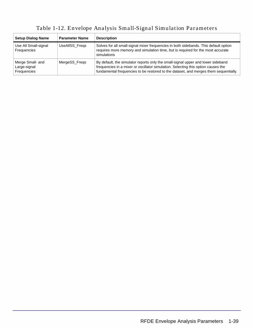
Use All Small-signal Frequencies
UseAllSS_Freqs Solves for all small-signal mixer frequencies in both sidebands. This default option requires more memory and simulation time, but is required for the most accurate simulations
Merge Small- and Large-signal Frequencies
MergeSS_Freqs By default, the simulator reports only the small-signal upper and lower sideband frequencies in a mixer or oscillator simulation. Selecting this option causes the fundamental frequencies to be restored to the dataset, and merges them sequentially.
Table 1-12. Envelope Analysis Small-Signal Simulation Parameters
Setup Dialog Name Parameter Name Description
RFDE Envelope Analysis Parameters 1-39

Circuit Envelope Simulation
Selecting a Harmonic Balance Convergence/Solver Technique
The Convergence / Solver parameters enable you to select a Direct or Krylov solver, or to allow the simulator to assign one automatically. The automatic selection is the default and recommended choice, since it allows the simulator to choose the most effective solver for each particular circuit. Newton’s method needs to solve a sequence of linear problems. If Newton’s method doesn’t converge or the convergence rate is too slow the Direct method will use arc-length continuation, while the Krylov method will use source stepping. The following table describes the parameter details. Names listed in the Parameter Name column are used in netlists.
Table 1-13. Envelope Analysis Convergence/Solver Parameters
Setup Dialog Name Parameter Name Description
Convergence Mode ConvMode
Automatic =Auto (Preferred) This is the default mode setting. It is both fast and robust, combining capabilities of the Basic and Advanced modes. This mode will automatically activate advanced features to achieve convergence. The Auto mode also allows for convergence at looser tolerances if the simulation does not meet the default tolerances. A warning message is given in the status window when this occurs, and it includes the tolerance level up to which convergence was achieved.
Robust =Advanced (Robust) Enables an advanced Newton solver. This mode is extremely robust, and ensures maximal KCL residual reduction at each iteration. It is recommended that the maximum number of iterations (MaxIters) be increased to the 50-100 range when this mode is selected.
Fast =Basic (Fast) Enables the basic Newton solver. It is fast and performs well for most circuits. For highly nonlinear circuits the basic mode may have difficulties converging. It is then recommended to switch to the Advanced convergence mode.
Max. iterations MaxIters The maximum number of Newton iterations to be performed. The simulation will iterate until it converges, an error occurs, or this limit is reached. The default and recommended option is Robust. You can also specify the number manually by choosing the Custom option and entering an integer. The larger the number is, the more robust the simulation will be.
1-40 RFDE Envelope Analysis Parameters
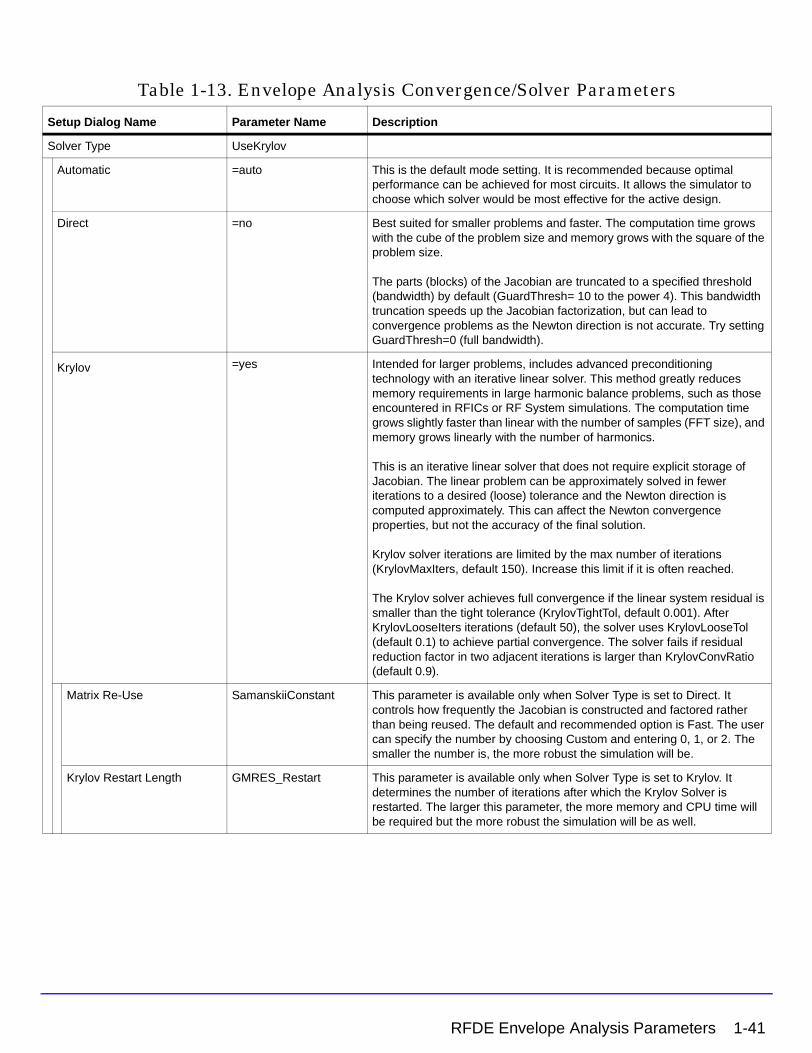
Solver Type UseKrylov
Automatic =auto This is the default mode setting. It is recommended because optimal performance can be achieved for most circuits. It allows the simulator to choose which solver would be most effective for the active design.
Direct =no Best suited for smaller problems and faster. The computation time grows with the cube of the problem size and memory grows with the square of the problem size.
The parts (blocks) of the Jacobian are truncated to a specified threshold (bandwidth) by default (GuardThresh= 10 to the power 4). This bandwidth truncation speeds up the Jacobian factorization, but can lead to convergence problems as the Newton direction is not accurate. Try setting GuardThresh=0 (full bandwidth).
Krylov =yes Intended for larger problems, includes advanced preconditioning technology with an iterative linear solver. This method greatly reduces memory requirements in large harmonic balance problems, such as those encountered in RFICs or RF System simulations. The computation time grows slightly faster than linear with the number of samples (FFT size), and memory grows linearly with the number of harmonics.
This is an iterative linear solver that does not require explicit storage of Jacobian. The linear problem can be approximately solved in fewer iterations to a desired (loose) tolerance and the Newton direction is computed approximately. This can affect the Newton convergence properties, but not the accuracy of the final solution.
Krylov solver iterations are limited by the max number of iterations (KrylovMaxIters, default 150). Increase this limit if it is often reached.
The Krylov solver achieves full convergence if the linear system residual is smaller than the tight tolerance (KrylovTightTol, default 0.001). After KrylovLooseIters iterations (default 50), the solver uses KrylovLooseTol (default 0.1) to achieve partial convergence. The solver fails if residual reduction factor in two adjacent iterations is larger than KrylovConvRatio (default 0.9).
Matrix Re-Use SamanskiiConstant This parameter is available only when Solver Type is set to Direct. It controls how frequently the Jacobian is constructed and factored rather than being reused. The default and recommended option is Fast. The user can specify the number by choosing Custom and entering 0, 1, or 2. The smaller the number is, the more robust the simulation will be.
Krylov Restart Length GMRES_Restart This parameter is available only when Solver Type is set to Krylov. It determines the number of iterations after which the Krylov Solver is restarted. The larger this parameter, the more memory and CPU time will be required but the more robust the simulation will be as well.
Table 1-13. Envelope Analysis Convergence/Solver Parameters
Setup Dialog Name Parameter Name Description
RFDE Envelope Analysis Parameters 1-41

Circuit Envelope Simulation
Advanced Krylov Parameters These parameters are available when Solver Type is set to Krylov. These parameters allow detailed configuration for the Krylov solver. Default values are recommended for optimal performance.
Max Iterations KrylovMaxIters Maximum number of GMRES iterations allowed. It is used to interrupt an otherwise infinite, loop in the case of poor or no convergence. The default is intentionally set to a large value of 150 to accommodate even slowly convergent iterations. You can still increase this number in cases where poor convergence may be improved and you are willing to allow more time for it.
Krylov Noise Tolerance KrylovSS_Tol Sets the tolerance for the Krylov solver when that solver is used either for small-signal harmonic balance analysis or for nonlinear noise analysis. It needs to be tight, and the default value is 1e-6. Larger values may lead to less accurate results, while further tightening may require longer simulation times.
Packing Threshold KrylovPackingThresh Used with Matrix Packing. Packing Threshold sets the bandwidth threshold for the packing. The default value is 1e-8. Set this to a larger value to increase the memory reduction.
Tight Tolerance KrylovTightTol The solver achieves full convergence if the Krylov solver residual is less than this tight tolerance setting (default=0.001).
Loose Tolerance KrylovLooseTol After the number of iterations specified by the parameter Loose Iterations, the solver then uses Loose Tolerance (default=0.1) to achieve partial convergence.
Loose Iterations KrylovLooseIters Sets the number of iterations allowed (default=50) to achieve convergence before using the Loose Tolerance value. When the number of Loose Iterations is reached, the solver then uses the Loose Tolerance value to achieve partial convergence.
Matrix packing KrylovUsePacking Directs the solver to use the technique known as spectral packing, which reduces the memory needed for the Jacobian, typically by 60-80%. The penalty is a longer computation time if no swapping is required. By default, this feature is turned off. You should turn on for extremely large problems in which the available RAM would not be able to accommodate the Jacobian.
Table 1-13. Envelope Analysis Convergence/Solver Parameters
Setup Dialog Name Parameter Name Description
1-42 RFDE Envelope Analysis Parameters
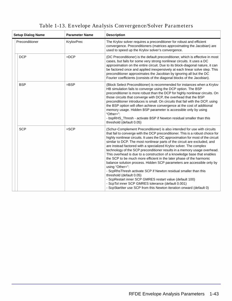
Preconditioner KrylovPrec The Krylov solver requires a preconditioner for robust and efficient convergence. Preconditioners (matrices approximating the Jacobian) are used to speed up the Krylov solver’s convergence.
DCP =DCP (DC Preconditioner) is the default preconditioner, which is effective in most cases, but fails for some very strong nonlinear circuits. It uses a DC approximation on the entire circuit. Due to its block-diagonal nature, it can be factored once and applied inexpensively at each linear solve step. This preconditioner approximates the Jacobian by ignoring all but the DC Fourier coefficients (consists of the diagonal blocks of the Jacobian).
BSP =BSP (Block Select Preconditioner) is recommended for instances when a Krylov HB simulation fails to converge using the DCP option. The BSP preconditioner is more robust than the DCP for highly nonlinear circuits. On those circuits that converge with DCP, the overhead that the BSP preconditioner introduces is small. On circuits that fail with the DCP, using the BSP option will often achieve convergence at the cost of additional memory usage. Hidden BSP parameter is accessible only by using “Other=”:- bspRHS_Thresh - activate BSP if Newton residual smaller than this threshold (default 0.05)
SCP =SCP (Schur-Complement Preconditioner) is also intended for use with circuits that fail to converge with the DCP preconditioner. This is a robust choice for highly nonlinear circuits. It uses the DC approximation for most of the circuit similar to DCP. The most nonlinear parts of the circuit are excluded, and are instead factored with a specialized Krylov solver. The complex technology of the SCP preconditioner results in a memory usage overhead. This overhead is due to a construction of a knowledge base that enables the SCP to be much more efficient in the later phase of the harmonic balance solution process. Hidden SCP parameters are accessible only by using “Other=”:- ScpRhsThresh activate SCP if Newton residual smaller than this threshold (default 0.05)- ScpRestart inner SCP GMRES restart value (default 100)- ScpTol inner SCP GMRES tolerance (default 0.001)- ScpStartIter use SCP from this Newton iteration onward (default 0)
Table 1-13. Envelope Analysis Convergence/Solver Parameters
Setup Dialog Name Parameter Name Description
RFDE Envelope Analysis Parameters 1-43
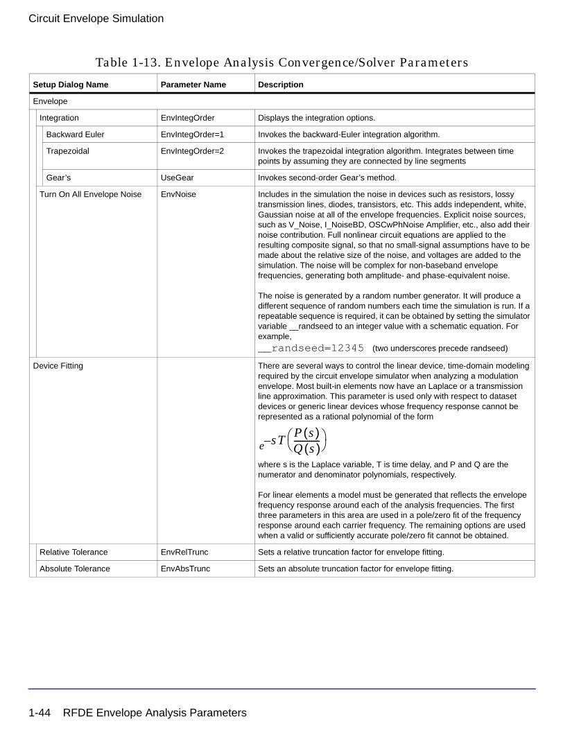
Circuit Envelope Simulation
Envelope
Integration EnvIntegOrder Displays the integration options.
Backward Euler EnvIntegOrder=1 Invokes the backward-Euler integration algorithm.
Trapezoidal EnvIntegOrder=2 Invokes the trapezoidal integration algorithm. Integrates between time points by assuming they are connected by line segments
Gear’s UseGear Invokes second-order Gear’s method.
Turn On All Envelope Noise EnvNoise Includes in the simulation the noise in devices such as resistors, lossy transmission lines, diodes, transistors, etc. This adds independent, white, Gaussian noise at all of the envelope frequencies. Explicit noise sources, such as V_Noise, I_NoiseBD, OSCwPhNoise Amplifier, etc., also add their noise contribution. Full nonlinear circuit equations are applied to the resulting composite signal, so that no small-signal assumptions have to be made about the relative size of the noise, and voltages are added to the simulation. The noise will be complex for non-baseband envelope frequencies, generating both amplitude- and phase-equivalent noise.
The noise is generated by a random number generator. It will produce a different sequence of random numbers each time the simulation is run. If a repeatable sequence is required, it can be obtained by setting the simulator variable __randseed to an integer value with a schematic equation. For example, __randseed=12345 (two underscores precede randseed)
Device Fitting There are several ways to control the linear device, time-domain modeling required by the circuit envelope simulator when analyzing a modulation envelope. Most built-in elements now have an Laplace or a transmission line approximation. This parameter is used only with respect to dataset devices or generic linear devices whose frequency response cannot be represented as a rational polynomial of the form
where s is the Laplace variable, T is time delay, and P and Q are the numerator and denominator polynomials, respectively.
For linear elements a model must be generated that reflects the envelope frequency response around each of the analysis frequencies. The first three parameters in this area are used in a pole/zero fit of the frequency response around each carrier frequency. The remaining options are used when a valid or sufficiently accurate pole/zero fit cannot be obtained.
Relative Tolerance EnvRelTrunc Sets a relative truncation factor for envelope fitting.
Absolute Tolerance EnvAbsTrunc Sets an absolute truncation factor for envelope fitting.
Table 1-13. Envelope Analysis Convergence/Solver Parameters
Setup Dialog Name Parameter Name Description
sT–eP s( )Q s( )------------
1-44 RFDE Envelope Analysis Parameters
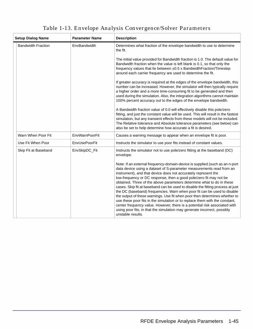
Bandwidth Fraction EnvBandwidth Determines what fraction of the envelope bandwidth to use to determine the fit.
The initial value provided for Bandwidth fraction is 1.0. The default value for Bandwidth fraction when the value is left blank is 0.1, so that only the frequency values that lie between ±0.5 x BandwidthFraction/Timestep around each carrier frequency are used to determine the fit.
If greater accuracy is required at the edges of the envelope bandwidth, this number can be increased. However, the simulator will then typically require a higher order and a more time-consuming fit to be generated and then used during the simulation. Also, the integration algorithms cannot maintain 100% percent accuracy out to the edges of the envelope bandwidth.
A Bandwidth fraction value of 0.0 will effectively disable this pole/zero fitting, and just the constant value will be used. This will result in the fastest simulation, but any transient effects from these models will not be included. The Relative tolerance and Absolute tolerance parameters (see below) can also be set to help determine how accurate a fit is desired.
Warn When Poor Fit EnvWarnPoorFit Causes a warning message to appear when an envelope fit is poor.
Use Fit When Poor EnvUsePoorFit Instructs the simulator to use poor fits instead of constant values.
Skip Fit at Baseband EnvSkipDC_Fit Instructs the simulator not to use pole/zero fitting at the baseband (DC) envelope.
Note: If an external frequency-domain-device is supplied (such as an n-port data device using a dataset of S-parameter measurements read from an instrument), and that device does not accurately represent the low-frequency or DC response, then a good pole/zero fit may not be obtained. Three of the above parameters determine what to do in these cases. Skip fit at baseband can be used to disable the fitting process at just the DC (baseband) frequencies. Warn when poor fit can be used to disable the output of these warnings. Use fit when poor then determines whether to use these poor fits in the simulation or to replace them with the constant, center frequency value. However, there is a potential risk associated with using poor fits, in that the simulation may generate incorrect, possibly unstable results.
Table 1-13. Envelope Analysis Convergence/Solver Parameters
Setup Dialog Name Parameter Name Description
RFDE Envelope Analysis Parameters 1-45
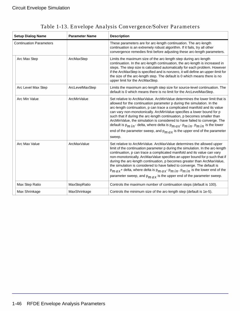
Circuit Envelope Simulation
Continuation Parameters These parameters are for arc-length continuation. The arc-length continuation is an extremely robust algorithm. If it fails, try all other convergence remedies first before adjusting these arc-length parameters.
Arc Max Step ArcMaxStep Limits the maximum size of the arc-length step during arc-length continuation. In the arc-length continuation, the arc-length is increased in steps. The step size is calculated automatically for each problem. However if the ArcMaxStep is specified and is nonzero, it will define an upper-limit for the size of the arc-length step. The default is 0 which means there is no upper limit for the ArcMaxStep.
Arc Level Max Step ArcLevelMaxStep Limits the maximum arc-length step size for source-level continuation. The default is 0 which means there is no limit for the ArcLevelMaxStep.
Arc Min Value ArcMinValue Set relative to ArcMaxValue. ArcMinValue determines the lower limit that is allowed for the continuation parameter p during the simulation. In the arc-length continuation, p can trace a complicated manifold and its value can vary non-monotonically. ArcMinValue specifies a lower bound for p such that if during the arc-length continuation, p becomes smaller than ArcMinValue, the simulation is considered to have failed to converge. The default is pmin- delta, where delta is pmax- pmin, pmin is the lower
end of the parameter sweep, and pmax is the upper end of the parameter
sweep.
Arc Max Value ArcMaxValue Set relative to ArcMinValue. ArcMaxValue determines the allowed upper limit of the continuation parameter p during the simulation. In the arc-length continuation, p can trace a complicated manifold and its value can vary non-monotonically. ArcMaxValue specifies an upper bound for p such that if during the arc-length continuation, p becomes greater than ArcMaxValue, the simulation is considered to have failed to converge. The default is pmax+ delta, where delta is pmax- pmin, pmin is the lower end of the
parameter sweep, and pmax is the upper end of the parameter sweep.
Max Step Ratio MaxStepRatio Controls the maximum number of continuation steps (default is 100).
Max Shrinkage MaxShrinkage Controls the minimum size of the arc-length step (default is 1e-5).
Table 1-13. Envelope Analysis Convergence/Solver Parameters
Setup Dialog Name Parameter Name Description
1-46 RFDE Envelope Analysis Parameters

Memory Management These parameters are available when Solver Type is Krylov.
Matrix Bandwidth(Guard Threshold)
GuardThresh The Jacobian matrix from the direct solver within the Newton solver is a block matrix. A block matrix is a matrix whose elements are matrices and vectors. The blocks of the Jacobian are truncated to a specified threshold by default. The default threshold (bandwidth) is set by Guard Threshhold, and its default option is Fast. The bandwidth truncation speeds up the Jacobian factorization and saves memory, but can lead to convergence problems due to an inaccurate Newton direction. In order to get the full bandwidth of the Jacobian blocks and improve the convergence, choose the Robust option.
FFT Options PackFFT Controls the frequency map packing for multitone Harmonic Balance. By default, when it is not explicitly set to yes or no by the user, the simulator enables it (sets it to yes).
Minimize Memory & Runtime PackFFT=yes Enables frequency map packing, which may improve the simulation speed and reduce memory consumption by using a smaller number of time samples (smaller FFTs), but at the potential loss of dynamic range and accuracy due to the aliased harmonics of the first fundamental now possibly landing on various mixing tones.
Minimize Aliasing PackFFT=no Disables frequency map packing to achieve most accurate results.
Waveform Memory Reduction
Use Dynamic Waveform Recalculation
RecalculateWaveForms Enables reuse of dynamic waveform memory instead of upfront storage on all waveforms. Small circuits might simulate a little slower, but not significantly
Use Compact Frequency Map
UseCompactFreqMap Enables a spectral compression, typically requiring less memory for individual waveforms.
Table 1-13. Envelope Analysis Convergence/Solver Parameters
Setup Dialog Name Parameter Name Description
RFDE Envelope Analysis Parameters 1-47
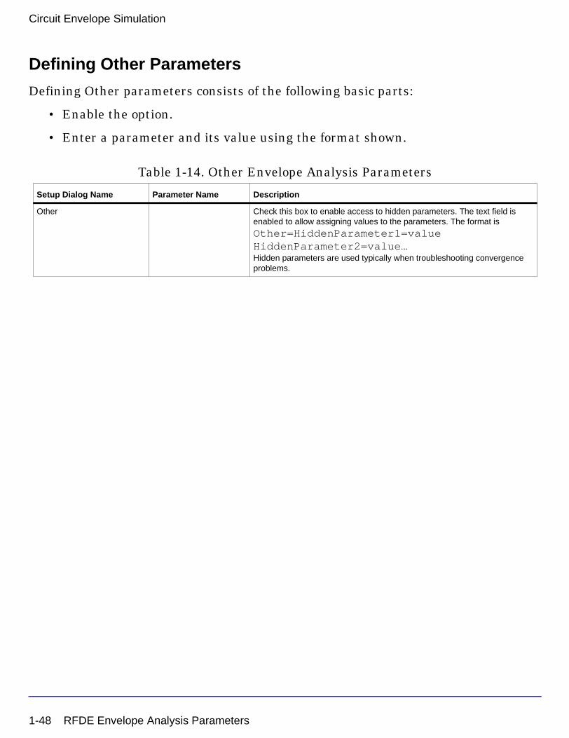
Circuit Envelope Simulation
Defining Other Parameters
Defining Other parameters consists of the following basic parts:
• Enable the option.
• Enter a parameter and its value using the format shown.
Table 1-14. Other Envelope Analysis Parameters
Setup Dialog Name Parameter Name Description
Other Check this box to enable access to hidden parameters. The text field is enabled to allow assigning values to the parameters. The format is
Other=HiddenParameter1=value HiddenParameter2=value... Hidden parameters are used typically when troubleshooting convergence problems.
1-48 RFDE Envelope Analysis Parameters
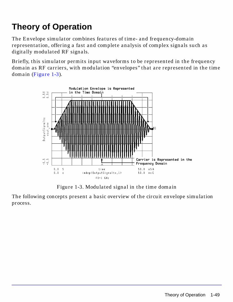
Theory of OperationThe Envelope simulator combines features of time- and frequency-domain representation, offering a fast and complete analysis of complex signals such as digitally modulated RF signals.
Briefly, this simulator permits input waveforms to be represented in the frequency domain as RF carriers, with modulation “envelopes” that are represented in the time domain (Figure 1-3).
Figure 1-3. Modulated signal in the time domain
The following concepts present a basic overview of the circuit envelope simulation process.
Theory of Operation 1-49
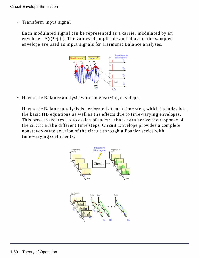
Circuit Envelope Simulation
• Transform input signal
Each modulated signal can be represented as a carrier modulated by an envelope - A(t)*ejf(t). The values of amplitude and phase of the sampled envelope are used as input signals for Harmonic Balance analyses.
• Harmonic Balance analysis with time-varying envelopes
Harmonic Balance analysis is performed at each time step, which includes both the basic HB equations as well as the effects due to time-varying envelopes. This process creates a succession of spectra that characterize the response of the circuit at the different time steps. Circuit Envelope provides a complete nonsteady-state solution of the circuit through a Fourier series with time-varying coefficients.
1-50 Theory of Operation

• Extract data from time domain
Selecting the desired harmonic spectral line (fc in this case), it is possible to analyze:
• Amplitude vs. time (oscillator start up, pulsed RF response, AGC transients)
• Phase (f) vs. time (t) (VCO instantaneous frequency (df/dt), PLL lock time)
• Amplitude and phase vs. time (constellation plots, EVM, BER)
Theory of Operation 1-51

Circuit Envelope Simulation
• Extract data from frequency domain
By applying FFT to the selected time-varying spectral line it is possible to analyze:
• Adjacent channel power ratio (ACPR)
• Noise power ratio (NPR)
• Power added efficiency (PAE)
• Reference frequency feedthrough in PLL
• Higher order intermods (3rd, 5th, 7th, 9th)
To describe the circuit envelope simulation process more specifically, in an envelope simulation each node voltage is represented by a discrete spectrum having time-varying Fourier coefficients. The set of spectral frequencies is user-defined; the amplitude and phase at each spectral frequency can vary with time, so the signal representing the harmonic is no longer limited to a constant, as it is with harmonic balance. Each spectral frequency can be thought of as the center frequency of a spectrum; the width of each spectrum is ±0.5/Time step. Figure 1-4 illustrates this, where the minimum envelope bandwidth is equal to the bandwidth of the modulation signal. In most cases the bandwidth of the modulation signal is much smaller than the lowest user-defined spectral frequency (which corresponds to the “carrier” frequency), unlike what is shown in the figure.
1-52 Theory of Operation

Figure 1-4. Spectra in the frequency domain
The bandlimited signal within each spectrum can contain periodic, transient, or random tones. The actual time-domain waveform is represented as a sum of carriers (with harmonics and intermodulation products), where each envelope can vary with time:
Here, v(t) is a voltage at any node in the circuit, including the input. The Fourier coefficients, Vk(t), are allowed to vary with time and may represent an arbitrary modulation of each carrier. Since each time-varying spectrum Vk(t) can be thought of as a modulation waveform with a center frequency fk, these are often referred to as “envelopes.” This spectrum may represent transient signals with continuous spectra, such as a digital modulation envelope over an RF carrier, or periodic signals with discrete spectral lines, such as the two RF tones required for intermodulation distortion analysis.
Figure 1-5 illustrates a modulated signal and the time-varying spectrum that results from the simulation. Any spectral component obtained from the simulation can be processed and displayed in amplitude, phase, I (the in-phase modulation component), or Q (the quadrature modulation component). By computing the Fourier transform of the spectral component, the simulator can present the spectrum around the component, as in a spectrum analyzer display.
v t( ) Vk t( )ej2πfkt
k 0=
N
∑real=
Theory of Operation 1-53
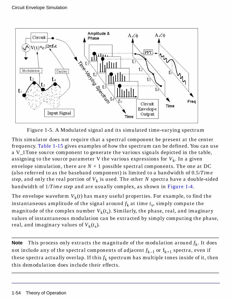
Circuit Envelope Simulation
Figure 1-5. A Modulated signal and its simulated time-varying spectrum
This simulator does not require that a spectral component be present at the center frequency. Table 1-15 gives examples of how the spectrum can be defined. You can use a V_1Tone source component to generate the various signals depicted in the table, assigning to the source parameter V the various expressions for Vk. In a given envelope simulation, there are N + 1 possible spectral components. The one at DC (also referred to as the baseband component) is limited to a bandwidth of 0.5/Time step, and only the real portion of Vk is used. The other N spectra have a double-sided bandwidth of 1/Time step and are usually complex, as shown in Figure 1-4.
The envelope waveform Vk(t) has many useful properties. For example, to find the instantaneous amplitude of the signal around fk at time ts, simply compute the magnitude of the complex number Vk(ts). Similarly, the phase, real, and imaginary values of instantaneous modulation can be extracted by simply computing the phase, real, and imaginary values of Vk(ts).
Note This process only extracts the magnitude of the modulation around fk. It does not include any of the spectral components of adjacent fk–1 or fk+1 spectra, even if these spectra actually overlap. If this fk spectrum has multiple tones inside of it, then this demodulation does include their effects.
1-54 Theory of Operation

This simple technique does not allow the demodulation of only one of the tones inside this fk spectrum and the exclusion of the others. To demodulate only one tone, first select the desired tone by using an appropriate filter in the circuit to be simulated. Also, note that because the baseband (DC) spectrum represents a real signal and not a complex envelope, its magnitude corresponds to taking the absolute value of that signal, and its phase is either 0 or 180 degrees.
Circuit Envelope and Frequency-Domain-Defined Devices
As the applications for wireless communications continue to grow, it is no longer possible to satisfy all modeling needs with standard, preconfigured models. Users need methods to define their own nonlinear models in either the time or the frequency domain. The frequency-domain-defined device (FDD) has been developed to allow a user to describe current and voltage spectral values directly, in terms of the algebraic relationships of other voltage and current spectral values.
Another trend in digital communication systems is the issue of timing, since it is increasingly common to encounter subsystems that behave in ways that cannot be modeled as time-invariant. Clocked systems, sampled systems, TDMA pulsed
Table 1-15. Examples of Defining a Spectrum around fk
# Formula that specifies the envelope Description of the signal in the time domain
1 Vk=1 Pure cosine: cos(2*pi*fk*time)
2 Vk=exp(j*pi/2) or polar(1,90) or 1*j Pure sine: sin(2*pi*fk*time)
3 Vk=A*exp(j*2*pi*fm*time+B) One tone (SSB) A*cos(2*pi*(fk+fm)*time+B)
4 Vk=A*exp(j*B); freq=1.1 GHz Same as (3) (assuming fk + fm = 1.1 GHz)
5 Vk=2*cos(2*pi*fm*time) Two tones (AM suppressed carrier)
6 Vk=exp(j*2*pi*fm*time) + exp(–j*2*pi*fm*time) Same as (5)
7 Vk=pulse(time,...); freq=fk+fm Pulsed RF at a frequency of fk + fm
8 Vk= –step(time – delay) A negative cosine wave, gated on at t=delay
9 Vk= (vreal(time)+
j*vimag(time))* exp(j*2*pi*fm*time)
I/Q modulated source centered at fk+fm. (vreal(), vimag()
user-defined functions)
10 Vk=(1 + vr1) * exp(j*2*pi*vr2) Amplitude- and noise-modulated source at fk. (vr1, vr2 are
user-defined randtime functions, not available in Release 1.0)
11 Vk=exp(j*2*pi*(–f0 + a0*time/2)*time) Chirped FM signal starting at fk – f0, rate = a0
Theory of Operation 1-55

Circuit Envelope Simulation
systems, and digitally controlled systems are all becoming more common, even in the RF and microwave area, and behavioral models must be able to include these effects. So, in addition to its frequency-domain modeling attributes, the FDD also allows the modeler to define trigger events, to sample voltages and currents at trigger events, and to generate outputs that are arbitrary functions of either the time of the trigger or of the complex spectral voltage and current values at these trigger events.
Circuit Envelope and Components
In general, any of the components available in Advanced Design System can be used in circuits where envelope simulations are performed. Some components lend themselves especially well to such circuit designs, such as n-state modulators and demodulators or spectral waveform sources.
Using Functions and Equations
Functions and equations can be placed in a schematic in the same manner as ADS components, and some are especially well-suited to envelope simulations and behavioral model designs. There is also a set of functions that can be used only with FDDs, and a set of variables that can be used only with SDDs; they, too, can facilitate digital communication designs where the envelope simulator is applied.
To use the Variables and equations component:
1. From the Data Items palette, select Var eqn (Variables and equations) and place it in the Schematic window.
2. Edit it and select the File Based option from the Variable or Equation Entry Mode drop-down list.
3. In the Data Access Component field, type the Instance Name—or select it from the drop-down list—of the DAC that points to the file containing the data of interest.
This makes it possible to use lists of data as component parameter values. Such data can also be used with n-state components to define the phase and amplitude of the various states. These components are especially efficient in envelope simulations, and dataset and list arrays simplify the entering of strings of data as parameter values.
1-56 Theory of Operation
Automatic Verification Modeling
Automatic Verification Modeling (AVM) is a user-selected mode of operation that can significantly speed up formerly lengthy cosimulations of Analog/RF circuits. This mode is also known as Fast Cosimulation. When this mode is enabled, the analog subcircuit is first characterized using a variety of Harmonic Balance simulations at the start of every Ptolemy simulation. Then during the actual Ptolemy simulation, this characterization data is used to predict the response of the subcircuit instead of performing the full circuit simulation at each time point.
Since this characterization is normally done at the start of every Ptolemy sweep based on the full circuit level schematic, the overall capability is basically the same as if the actual circuit level representation is used throughout the cosimulation. For example, optimization of circuit level parameters, or swept parameters including bias, temperature or swept carrier frequency will continue to operate as expected. These capabilities do not exist when the circuit is manually replaced with behavioral models.
This ability to predict the modulated response based on the Harmonic Balance characterization relies on the fact that many circuits, when used in relatively narrow band modulated applications, can have their nonlinearity represented as a static nonlinearity that is strictly a function of the instantaneous amplitude of the carrier. Many of these circuits, such as amplifiers and mixers, have little, if any, frequency response over the modulation bandwidth of interest. Any frequency response effects that do exist can then often be represented as either a linear filter on either the input or the output of the nonlinearity.
Each output of the Analog/RF subcircuit is then characterized by the following equation:
The functions are determined by the swept amplitude Harmonic Balance simulation. The HarmGain is the harmonic gain determined from the harmonic indices of the input and output frequencies.
If phase characterization has been enabled, by setting the “Num. of phase pts” parameter to a non-zero value, then each output is characterized by this modified equation:
Outk Pk InputMag( ) Pk 0( )–( ) ejInputPhase HarmGain×× Pk 0( )+=
k mag( )
Outk Pk InputMag InputPhase,( )=
Theory of Operation 1-57
Circuit Envelope Simulation
In this case, functions are determined by a two dimensional swept amplitude and swept phase Harmonic Balance simulation.
If the subcircuit nonlinearities are a function the input phase, as in a nonlinear IQ demodulator, then the amplitude only characterization is not accurate and the two dimensional amplitude and phase characterization must be used. However, if the IQ Modem phase characteristics are linear, then the IQ input or output pair can be identified in the Node Names section, and the Magnitude only characterization can still be used, as the HarmGain value is then set to 1. This requires that the I/Q pair be properly identified such that there are no phase inversions introduced, since this would require a harmonic gain of -1.
Note that the magnitude only characterization assumes the output phase can be determined from the harmonic indices of the input and output frequencies. In certain rare cases, this can be ambiguous. For example, if the input frequency is fund1 and the output frequency is 2*fund1, then the simulator assumes the output signal is generated by a doubling the input frequency and so the input phase is doubled. However, if this 2*fund1 output frequency is actually generated by mixing with another LO source at the fund1 frequency and so the phase relationship is supposed to be linear, then the AVM (Fast Cosim) results will be incorrect. If the mixer LO is operating at an independent fund2 frequency, with a mixer output at fund1 + fund2, then the HarmGain of 1.0 is correctly determined. So, as with the IQ demodulator, if there are circuit sources operating at the same frequency as the input signal, then caution should be used when enabling this AVM (Fast Cosim) mode, and the two dimensional amplitude and phase characterization may be required.
In addition to the swept amplitude characterization, the AVM characterization also includes a small signal Harmonic Balance frequency sweep. In this case, the input amplitude is set to 0, and the small signal frequency is swept between +/- 0.5/TimeStep. Note that even though the input amplitude is set to 0, a nonlinear analysis is still being done so any frequency translation effects due to internal mixers will be fully captured. An impulse response representing this frequency response can then be generated, and then, as the user’s choice, placed on either the input or the output of the nonlinear block. An additional delay can also be added to the frequency response, so that the impulse can be made a more accurate representation of the frequency response. The user should set the number of frequency points high enough that any frequency response deviations are sufficiently sampled (a minimum of 4 samples every 360 degrees). The maximum duration of the impulse response will be about 0.75/FreqSpacing, where
k mag phase,( )
1-58 Theory of Operation

N is determined so that 2N is just larger than the user-specified number of frequency points. So, if frequency compensation is needed, the number of frequency points should generally be greater than the maximum impulse response time of the circuit around the carrier frequency plus any additional Delay specified in the Cosim Implementation block, both normalized by the Circuit Envelope TimeStep value.
In addition to the amplitude and frequency response characterization, nonlinear noise characterization is also done. A single value for the equivalent input noise for each output is determined and then added to the input signal prior to the above nonlinear and frequency response effects. In the case of multiple outputs, these equivalent noise sources are uncorrelated. So any correlation of the Analog/RF subcircuit added noise between multiple outputs is lost during this AVM (Fast Cosim) mode. Whether or not this noise characterization is done and implemented is determined by the standard EnvNoise parameter set in the Envelope simulation.
In certain cases, the time spent doing this characterization can be eliminated if the user requests that the simulator use previous characterization. Once this mode is selected, then it is the responsibility of the user to make sure that the previous characterization is still valid, and that circuit parameters have not been changed, perhaps by optimization, biases have not changed, carrier frequencies have not changed, etc. The circuit should not have changed its connectivity within the Ptolemy environment and names of the OutputSelectors cannot have changed either. Also, the format and data in the dataset must be in the same expected configuration as when it was written by simulator.
In addition to the characterization and implementation portion of the AVM (Fast Cosim) mode, there is also a user selectable verification step. If the user specifies a non-zero verification Stop Time, then the normal Circuit Envelope simulation is performed in parallel with the fast cosimulation predictions. The error over this verification is then computed and output to determine how well these predictions are performing. If the behavior is unacceptable, as determined by the Accept Tolerance, then the AVM (Fast Cosim) will be disabled and only the normal Circuit Envelope results will be used. Clearly, if used, this verification time should be set long enough to include a representative portion of the input signal. This may need to take into account the fact that many sources, due to channel filtering, take a while to generate their full amplitude outputs.
FreqSpacing 1
2N TimeStep×
------------------------------------------=
Theory of Operation 1-59
Circuit Envelope Simulation
AVM Limitations
Though you may have selected the AVM (Fast Cosim) mode, it may be disabled for the following reasons:
• Verification was enabled but performance did not meet acceptance level.
• There was more than one input to the Analog/RF subcircuit from Ptolemy and the user did not specify the active input node name.
• The Envelope analysis includes an oscillator analysis.
• The input frequency was a mixing term and not harmonically related to a single fundamental.
• One of the Envelope OutSelectors was in AllPass mode.
• The input frequency is baseband and does not have a non-zero carrier frequency and no IQ input pairs were identified.
• The input frequency does not exactly match an Envelope analysis frequency.
• There was a problem reading the previously generated dataset.
Additional limitations of the AVM (Fast Cosim) mode, that may not be automatically detected by the simulator unless verification is enabled, include:
• Envelope analyses parameters such as the Freq parameters should not be swept or optimized.
• Do not use the AllPass mode in the EnvOutSelector component when using AVM (Fast Cosim) mode.
1-60 Theory of Operation

Troubleshooting a SimulationThis section presents suggestions for using this simulator and improving the accuracy of results.
Increasing Accuracy Easily
In general, accuracy is increased and aliasing reduced when the signal of greatest amplitude is entered as the Freq[1] parameter, and lower-amplitude signals are entered as Freq[2], Freq[3], and so on.
Improving Mixer IMD Measurement Accuracy and Speed
Prior to the invention of the Krylov subspace solver (available in harmonic balance simulation), Circuit Envelope was the recommended choice for mixer IMD (intermodulation distortion) measurements. Now the Krylov option appears to provide faster solutions for this application. Nevertheless, when the envelope simulator is used, there are several ways to improve accuracy and speed. Also, Maximum mixing order can have a profound effect on simulation results; in general, set Maximum mixing order to a low value and increase it until the simulation produces marginal differences in results.
Using the Circuit Envelope Simulator to Analyze an Oscillator
This simulator can support the simulation of oscillator circuits and subsystems, through the Oscillator analysis options. The oscillator options work as follows:
• If Oscillator analysis is disabled, the envelope simulation proceeds as normal and any oscillations, if present, will build up from some initial value. The analysis frequencies and time step must be set to ensure that the oscillator’s instantaneous frequency is well within one of the envelope bandwidths being simulated. This can be either the baseband (DC) envelope or any of the fundamental, harmonic, or mixing-term analysis-frequency envelopes. Multiple oscillations can be simulated as well, as long as each one is within an analysis envelope.
Troubleshooting a Simulation 1-61
Circuit Envelope Simulation
• When the transient buildup is being simulated, a tickler voltage is usually needed in the same envelope as the actual oscillator frequency, to define an initial start-up value. This value can be set by a low-level transient source that is disabled after the first few time samples. Alternatively, a noise source or resistor noise can also be used. For the oscillator control elements, the option Turn on all noise is enabled. This will cause devices with noise in the oscillator loop to generate the white noise that will provide the required tickler stimulus.
• If Oscillator analysis is enabled, then a normal harmonic-balance oscillator simulation is automatically performed prior to the first time step (refer to the chapter “Harmonic Balance Basics” in the Harmonic Balance Simulation documentation). The results of this simulation determine and set the analysis frequency value to the steady-state oscillator frequency. If the oscillation frequency does not change significantly during its buildup, this often allows larger time steps to be used. This is because the envelope bandwidth does not have to include any uncertainty as to the oscillator’s final frequency value.
• If Oscillator analysis is enabled, you may reset the oscillator voltage solution to zero by selecting Calculate oscillator startup transient, so that the transient buildup can be simulated. If this option is not enabled, the time-domain solution begins at the steady-state solution, the transient buildup time is skipped, and the oscillator can immediately start responding properly to any external modulation. Note that Oscillator analysis affects only the initial simulation, and is disabled once the envelope simulation begins.
Using the Circuit Envelope Simulator to Analyze Noise
Noise in envelope simulations can be added as random time voltages and currents. Noise can originate from circuit components such as resistors or noise sources. The full, nonlinear circuit equations are applied to this composite signal of random voltages and currents, so no small-signal assumptions about the relative size of the noise are required.
Setting the option Turn on all noise (under the Env Params tab) enables white noise from many devices in the circuit to be included in the simulation. The noise sources that are included in the circuit are also included in the simulation. They add white, Gaussian noise at all frequencies in the analysis envelope. The noise voltages will be complex for non-baseband envelope frequencies, generating both amplitude and phase equivalent noise.
1-62 Troubleshooting a Simulation

Convolution Techniques Used in Circuit Envelope
In Circuit Envelope, the response within the envelope bandwidth (1/timestep) around each of the Harmonic Balance frequencies (including DC) needs to be represented in the time domain. The advantage here over a transient simulation is that the entire frequency response need not be represented in the time domain, and if the envelope bandwidth is relatively small, then a simple fit or a constant is sufficient to represent the response. And since a different constant could be used for each carrier, it maintains good accuracy at the exact Harmonic Balance frequencies.
A consequence of this method is that any components which are characterized in the frequency domain need to have their response converted to the time domain for the portions of their frequency response which fall within the envelope bandwidth.
By default, the Circuit Envelope simulator uses recursive convolution for this task, which first tests to see if the frequency response is described by a rational polynomial. If it is not, the simulator then tries to fit the frequency response to a rational polynomial (with no delay) around each carrier. If this fails, a poor fit warning is generated and the simulation will either proceed with the best fit or just use the center frequency constant, depending on the setting in the analysis control.
Impulse convolution can be used, but it is currently only available for certain components such as S1P_Eqn, Y1P_Eqn, or Z1P_Eqn. These components have an ImpDeltaFreq parameter, and an appropriate value must be entered for the parameter to use impulse convolution. However, recursive convolution has priority over impulse convolution, even for such components, if the frequency response is described by a rational polynomial.
Troubleshooting a Simulation 1-63

Circuit Envelope Simulation
1-64 Troubleshooting a Simulation

Index
AABM_ActiveInputNode, 1-22ABM_AmpPts, 1-20ABM_Delay, 1-21ABM_FreqComp, 1-21ABM_FreqPts, 1-21ABM_IQ_Nodes, 1-22ABM_MaxPower, 1-20ABM_Mode, 1-20ABM_PhasePts, 1-21ABM_ReUseData, 1-21ABM_VTime, 1-22ABM_VTol, 1-22advantages, 1-4over Harmonic Balance, 1-4Annotation (RFDE), 1-27, 1-28applications, 1-2ArcLevelMaxStep, 1-46ArcMaxStep, 1-46ArcMaxValue, 1-46ArcMinValue, 1-46Automatic Verification Modeling (fast
cosimulation)limitations, 1-60overview, 1-57parameters (ADS), 1-20
AVM, 1-20
Bbandwidth fraction
in circuit envelope simulations, 1-17, 1-45BandwidthForNoise, 1-36
CCarrierFreq, 1-35CarrierIndex, 1-35Circuit Envelope simulations
and FDDs, 1-55and oscillator simulations (ADS), 1-19and oscillator simulations (RFDE), 1-32envelope formulas, 1-55in noise analysis, 1-62of oscillators, 1-61overview, 1-6performing, 1-5
theory of operation, 1-49troubleshooting, 1-61using V_1Tone source components, 1-54versus harmonic balance, 1-52
Circuit Envelope simulatorbandwidth fraction, 1-17, 1-45device fitting, 1-17, 1-44parameters (ADS), 1-12-1-24parameters (RFDE), 1-25-1-48
ConvMode, 1-40cosimulation, fast. See Automatic
Verification Modeling
Ddevice fitting
in circuit envelope simulations, 1-17, 1-44DevOpPtLevel, 1-23, 1-28
EEnvAbsTrunc, 1-17, 1-44EnvBandwidth, 1-17, 1-45envelope simulations. See Circuit
Envelope simulationsEnvIntegOrder, 1-16, 1-44EnvNoise, 1-16, 1-44EnvRelTrunc, 1-17, 1-44EnvSkipDC_Fit, 1-18, 1-45EnvUsePoorFit, 1-18, 1-45EnvWarnPoorFit, 1-17, 1-45
Ffast cosimulation. See Automatic
Verification ModelingFDDs
using with Circuit Envelope simulations, 1-55
Freq, 1-14, 1-27FreqForNoise, 1-33FundIndex, 1-32FundOversample, 1-23
GGMRES_Restart, 1-41GuardThresh, 1-47
Index-1
HHarm, 1-32harmonic balance simulations, 1-41HBAHB (ADS), 1-18HBAHB (RFDE)
user-supplied initial guess, 1-29using with TAHB, 1-29
HBAHB_Enable, 1-30
II (in-phase modulation component), 1-53IMD (intermodulation distortion), 1-7
using circuit envelope simulations, 1-1IncludePortNoise, 1-36InFile, 1-31Initial Guess (ADS), 1-18Initial Guess (RFDE), 1-29InputFreq, 1-35intermodulation distortion (IMD), 1-7IV_RelTol, 1-30
KKrylov solver, 1-41KrylovLooseIters, 1-42KrylovLooseTol, 1-42KrylovMaxIters, 1-42KrylovPackingThresh, 1-42KrylovPrec, 1-43KrylovSS_Tol, 1-42KrylovTightTol, 1-42KrylovUsePacking, 1-42
Llimitation of Circuit Envelope, 1-11
MMaximum Mixing Order, 1-27Maximum mixing order, 1-14MaxIters, 1-40MaxOrder, 1-14, 1-27MaxShrinkage, 1-46MaxStepRatio, 1-46MaxTimeStep, 1-30memory management, 1-47MergeSS_Freqs, 1-39mixers
finding intermodulation distortion (IMD), 1-7
NNode, 1-32noise
in Circuit Envelope simulations, 1-16, 1-44
produced by random number generator, 1-16, 1-44
NoiseInputPort, 1-35NoiseNode, 1-34NoiseOutputPort, 1-35NoiseThresh, 1-36NumOctaves, 1-32
OOrder, 1-14, 1-27OscFundIndex, 1-19OscHarmNum, 1-19oscillator simulations
and envelope simulations (ADS), 1-19and envelope simulations (RFDE), 1-32and oscillator ports (ADS), 1-19and oscillator ports (RFDE), 1-32OscPort (RFDE), 1-32OscPort2 (RFDE), 1-32OscProbe (RFDE), 1-32selecting analysis method (RFDE), 1-32
oscillatorsanalyzed by Circuit Envelope, 1-61calculating startup transient, 1-19, 1-32
OscNodeMinus, 1-19OscNodePlus, 1-19OscOctSrch, 1-19OscOctStep, 1-19OscPort
setting analysis method (RFDE), 1-32OscPortName, 1-19, 1-32OscProbe
setting analysis method (ADS), 1-19setting analysis method (RFDE), 1-32
OutFile, 1-31Oversample, 1-23, 1-27
PPackFFT, 1-47parameters (ADS), 1-12-1-24
ABM_ActiveInputNode, 1-22ABM_AmpPts, 1-20ABM_Delay, 1-21
Index-2

ABM_FreqComp, 1-21ABM_FreqPts, 1-21ABM_IQ_Nodes, 1-22ABM_MaxPower, 1-20ABM_Mode, 1-20ABM_PhasePts, 1-21ABM_ReUseData, 1-21ABM_VTime, 1-22ABM_VTol, 1-22AVM, 1-20DevOpPtLevel, 1-23EnvAbsTrunc, 1-17EnvBandwidth, 1-17EnvIntegOrder, 1-16EnvNoise, 1-16EnvRelTrunc, 1-17EnvSkipDC_Fit, 1-18EnvUsePoorFit, 1-18EnvWarnPoorFit, 1-17Freq, 1-14FundOversample, 1-23MaxOrder, 1-14Order, 1-14OscFundIndex, 1-19OscHarmNum, 1-19OscNodeMinus, 1-19OscNodePlus, 1-19OscOctSrch, 1-19OscOctStep, 1-19OscPortName, 1-19Oversample, 1-23ResetOsc, 1-19StatusLevel, 1-15Step, 1-14Stop, 1-14SweepOffset, 1-16UseGear, 1-16
parameters (RFDE), 1-25-1-48ArcLevelMaxStep, 1-46ArcMaxStep, 1-46ArcMaxValue, 1-46ArcMinValue, 1-46BandwidthForNoise, 1-36CarrierFreq, 1-35CarrierIndex, 1-35ConvMode, 1-40DevOpPtLevel, 1-28EnvAbsTrunc, 1-44
EnvBandwidth, 1-45EnvIntegOrder, 1-44EnvNoise, 1-44EnvRelTrunc, 1-44EnvSkipDC_Fit, 1-45EnvUsePoorFit, 1-45EnvWarnPoorFit, 1-45Freq, 1-27FreqForNoise, 1-33FundIndex, 1-32GMRES_Restart, 1-41GuardThresh, 1-47Harm, 1-32HBAHB_Enable, 1-30IncludePortNoise, 1-36InputFreq, 1-35IV_RelTol, 1-30KrylovLooseIters, 1-42KrylovLooseTol, 1-42KrylovMaxIters, 1-42KrylovPackingThresh, 1-42KrylovPrec, 1-43KrylovSS_Tol, 1-42KrylovTightTol, 1-42KrylovUsePacking, 1-42MaxIters, 1-40MaxOrder, 1-27MaxShrinkage, 1-46MaxStepRatio, 1-46MaxTimeStep, 1-30MergeSS_Freqs, 1-39Node, 1-32NoiseInputPort, 1-35NoiseNode, 1-34NoiseOutputPort, 1-35NoiseThresh, 1-36NumOctaves, 1-32Order, 1-27OscPortName, 1-32Oversample, 1-27PackFFT, 1-47PhaseNoise, 1-33, 1-36RecalculateWaveForms, 1-47ResetOsc, 1-32SamanskiiConstant, 1-41SaveToDataset, 1-30SortNoise, 1-36SS_Plan, 1-38
Index-3

StatusLevel, 1-28SteadyStateMinTime, 1-30Step, 1-26Steps, 1-32Stop, 1-26StopTime, 1-30Sweep Plan, 1-34, 1-38TAHB_Enable, 1-30Use Initial Guess, 1-31UseAllSS_Freqs, 1-39UseCompactFreqMap, 1-47UseGear, 1-44UseKrylov, 1-41Write Final Solution, 1-31
PhaseNoise, 1-33, 1-36
QQ (quadrature modulation component),
1-53
Rrandom number generator, 1-16, 1-44RecalculateWaveForms, 1-47ResetOsc, 1-19, 1-32Restart, 1-31
SSamanskiiConstant, 1-41SaveToDataset, 1-30simulation parameters
Circuit Envelope simulation (ADS), 1-12-1-24
Circuit Envelope simulation (RFDE), 1-25-1-48
SortNoise, 1-36SS_Plan, 1-38StatusLevel, 1-15, 1-28SteadyStateMinTime, 1-30Step, 1-14, 1-26Steps, 1-32Stop, 1-14, 1-26StopTime, 1-30Sweep Plan parameters (RFDE), 1-34,
1-38SweepOffset, 1-16
TTAHB (ADS), 1-18
TAHB (RFDE)parameter details, 1-29
TAHB_Enable, 1-30third-order intercept (TOI)
using circuit envelope simulations, 1-1
UUse Initial Guess parameter, 1-31UseAllSS_Freqs, 1-39UseCompactFreqMap, 1-47UseGear, 1-16, 1-44UseInFile, 1-31UseKrylov, 1-41UseOutFile, 1-31
VV_1Tone source components
in Circuit Envelope simulations, 1-54verification. See Automatic Verification
Modeling
WWrite Final Solution, 1-31
Index-4