cherry creek sediment analysis technical … · cherry creek sedimentation study reservoir to pine...
TRANSCRIPT
CHERRY CREEK SEDIMENT ANALYSIS
TECHNICAL MEMORADA
Collection of investigations prepared by George K Cotton Consulting, Inc.

C h e r r y C r e e k S e d i m e n t a t i o n S t u d y R e s e r v o i r t o P i n e L a n e
P r o j e c t D a t a a n d E v a l u a t i o n
November 2010 Prepared for: Southeast Metropolitan Stormwater Authority 76 Inverness Drive Englewood, Colorado Submitted to: Ms. Molly Trujillo, P.E. Prepared by:
GK COTTON CONSULTING, INC 10290 S. Progress Way, #205 PO Box 1060 Parker, CO 80134-1060

GK COTTON CONSULTING, INC. PAGE 2
C H E R RY C R E E K S E D I M E N TAT I O N S T U DY
PROJECT DATA AND EVALUATION
Table of Contents
Introduction ....................................................................................................................... 3
Period of Record ........................................................................................................................ 3
Description of the Study Area .................................................................................................... 4
Geology ............................................................................................................................. 5
Flow Data .......................................................................................................................... 6
Stream Gages ............................................................................................................................. 6
Stream Gage Statistics................................................................................................................ 8
Urban Development ................................................................................................................. 12
Inflow Time Series .................................................................................................................... 14
Stream and Valley Topography ........................................................................................ 17
Terrain Models ......................................................................................................................... 17
Channel Geometry ................................................................................................................... 17 Longitudinal Slope ....................................................................................................................................... 17 Stream Sections ........................................................................................................................................... 18
Sediment Surveys ............................................................................................................. 19
Alluvial Sediment Gradations ................................................................................................... 19 Bed Material ................................................................................................................................................ 19 Bank Material............................................................................................................................................... 20
Reservoir Sedimentation .......................................................................................................... 21
Channel Erosion ....................................................................................................................... 21
Information From Other Studies ...................................................................................... 23
Appendix A. Site Photos and Location Maps .................................................................... 25
Appendix B. Channel Sediment Samples .......................................................................... 33
Appendix C. Extracts from Other Studies .......................................................................... 44

GK COTTON CONSULTING, INC. PAGE 3
INTRODUCTION
This paper describes the data that was collected in support of analysis of the sediment transport in the Cherry Creek above Cherry Creek Lake. The data gathering effort focused on the segment of the Cherry Creek from the Pine Drive bridge in Parker, Colorado to the State Park perimeter road within the dam reservoir. Data gathering also includes sedimentation data for the reservoir pool itself.
Categories of data that were pursued for the project included: the surface geology; hydrology of the stream segment; topographic description of the stream channel and valley; and, measurements of sedimentation and erosion for the stream channel and reservoir pool. Published reports are discussed briefly in the context of what data they provide.
PERIOD OF RECORD
The period of data on the Cherry Creek is relatively recent and begins in 1940. This is ten years prior to the completion of the Cherry Creek dam by the U.S. Army Corps of Engineers in 1950. Prior to this period of data collection, we have only a qualitative understanding of the hydrologic history within the Cherry Creek watershed.
Western civilization has impacted the Cherry Creek basin for about 200 years. After the Lewis and Clark Expedition (1804 – 1806), the commercial fur trade expanded onto the plains west of the Mississippi River and later into the Rocky Mountains. The large-scale removal of beaver from western streams (no doubt including the Cherry Creek) impacted basin water storage, the extent of wetlands, and the character of riparian vegetation. Settlement of the Cherry Creek began in the 1870s and included the expansion of ranching throughout the watershed and the development of some irrigated farming in the valley. Over-grazing and periods of sustained drought in the Platte River basin impacted riparian areas of the Cherry Creek. Government sponsored erosion control programs began in the mid-1930’s to help restore the lost productivity of basin rangelands due to gully erosion.
The drought on the plains of the United States in the late 1930’s was the longest, driest and hottest of the 20th Century. Newly available rural electric power permitted deeper pumping of groundwater, which mitigated some of the drought impact within the Cherry Creek basin. The unregulated use of alluvial groundwater may be the reason for low base-flows in the Cherry Creek at the Melvin gage. Thus, at the beginning of the period of record for this study the basin hydrology was in a stressed state. Likewise, the riparian environment of stream channels was probably also in a stressed condition. The 1950s saw another period of sustained drought in the basin. So, the early period of the flow record reflects severe drought conditions and the unregulated use of alluvial groundwater.
Within the period of record, exurban development began on lands south of Cherry Creek Lake in the mid-1960s, which was followed by larger suburban development in the 1970’s. Urbanization continues to expand steadily, mostly in the portions of the basin north of about Franktown. Water supply for this development has to date been largely from deep community wells that have been developed into the lower Dawson and Denver formations. This supplemental water enters the Cherry Creek via wastewater discharges and tailwater runoff from lawn irrigation. In addition, the increased impervious area that is associated with the urban development diverts rainwater that would have infiltrated to drainageways that are tributary to the Cherry Creek.
Because of the intense use of surface and groundwater resources, the State of Colorado strictly administers water rights on the Cherry Creek basin. As a result, base flows in the period of record may not accurately reflect the current water rights administration.

GK COTTON CONSULTING, INC. PAGE 4
DESCRIPTION OF THE STUDY AREA
The study segment of the Cherry Creek is about eight (8.0) miles long. In this distance the valley of the Cherry Creek falls about 190 feet and has an average grade of 23.8 feet per mile (0.0045 feet/foot).
Figure 1. Approximate Limits of Study Segment (Section grid is approximately 1.0 mile)
The study segment is with the jurisdictions of Arapahoe Country and Douglas County. Both counties have completed detailed planning for the Cherry Creek stream corridor. The reservoir land is owned by the U.S. Army Corps of Engineers which leases the land within the reservoir to Colorado State Parks. City jurisdictions within the study segment include the Centennial, Aurora, and Parker.
Major tributaries that confluence with the Cherry Creek in this segment are Piney Creek, Happy Canyon Creek, and Baldwin Gulch / Newlin Gulch (right and left bank tributaries that confluence with the Cherry Creek at nearly the same location). The drainage area of the Cherry Creek at the Baldwin Gulch confluence is 310 square miles and at the reservoir it is 360 square miles.
N

GK COTTON CONSULTING, INC. PAGE 5
GEOLOGY
One of the reasons that the study limits were chosen is that the geology of the segment is relatively consistent. Each side of the Cherry Creek valley has distinctly different characteristics. Near the floodplain, the east side of the valley is composed of aeolian (wind-blown) sands (Qes) that are more uniform in nature than alluvial sediments. Upper portions of the east valley are within the Dawson formation (Tkd and Tkda), which formed as a series of ancient coalesced alluvial fans that overlie the Denver formation.
The west side of the valley consists of colluvial deposits that are derived from erosion of the Castle Rock conglomerate (Tkr) and Denver formation (Tkd). The Louviers alluvium (Qlo) borders much of the west valley and forms a gravelly terrace that is about 60 feet above the modern valley of the Cherry Creek.
With the exception of the aeolian sands, erosion of these base formations produces mostly coarse sands with some gravel sediments.
Figure 2. Segment Geology (USGS I-856-H Version 1.1 “Geologic Map of the Greater Denver Area, Front Range Urban Corridor, Colorado” by D.E. Trimble and M.N. Machette)

GK COTTON CONSULTING, INC. PAGE 6
FLOW DATA
STREAM GAGES
There are three Cherry Creek steam flow gages near the study segment. Records include mean daily flow and annual flow peaks. USGS metadata for each site is provided in Table 1 (a, b and c). The Melvin gage ceased operation at the end of water year 1969 and resumed briefly May and September of 1984. The CC-10 gage is located at the crossing of the state park perimeter road near the location of the previous Melvin gage. This gage has operated continuously since January 1992.
Table 1a. USGS 06712500 CHERRY CREEK NEAR MELVIN, CO. DESCRIPTION:
Latitude 39°36'18", Longitude 104°49'19" NAD27 Arapahoe County, Colorado, Hydrologic Unit 10190003 Drainage area: 360 square miles Datum of gage: 5,608.21 feet above sea level NGVD29.
AVAILABLE DATA: Data Type Begin Date End Date Count
Daily Data
Discharge, cubic feet per second 1939-10-01 1984-09-24 11075 Daily Statistics Discharge, cubic feet per second 1939-10-01 1984-09-24 11075 Monthly Statistics Discharge, cubic feet per second 1939-10 1984-09 Annual Statistics Discharge, cubic feet per second 1940 1984 Peak streamflow 1933-08-03 1969-08-21 30 Field measurements 1985-10-16 1985-12-16 10 Field/Lab water-quality samples 1964-12-03 1986-09-24 31

GK COTTON CONSULTING, INC. PAGE 7
Table 1b. USGS 393109104464500 CHERRY CREEK NEAR PARKER, CO DESCRIPTION:
Latitude 39°31'09", Longitude 104°46'45" NAD27 Douglas County, Colorado, Hydrologic Unit 10190003 Drainage area: 287 square miles Datum of gage: 5,805 feet above sea level NGVD29.
AVAILABLE DATA: Data Type Begin Date End Date Count
Daily Data
Discharge, cubic feet per second 1991-10-01 2010-10-26 6966 Daily Statistics Discharge, cubic feet per second 1991-10-01 2010-04-28 6785 Monthly Statistics Discharge, cubic feet per second 1991-10 2010-04 Annual Statistics Discharge, cubic feet per second 1992 2010 Peak streamflow 1992-07-12 2009-06-23 18 Field measurements 1991-10-22 2010-10-04 251 Field/Lab water-quality samples 1991-12-03 2003-03-17 160
Table 1c. USGS 06712000 CHERRY CREEK NEAR FRANKTOWN, CO. DESCRIPTION:
Latitude 39°21'21", Longitude 104°45'46" NAD27 Douglas County, Colorado, Hydrologic Unit 10190003 Drainage area: 169 square miles Datum of gage: 6,150.00 feet above sea level NGVD29.
AVAILABLE DATA:
Data Type Begin Date End Date Count Daily Data
Discharge, cubic feet per second 1939-11-21 2010-10-26 25908 Daily Statistics Discharge, cubic feet per second 1939-11-21 2010-04-15 25714 Monthly Statistics Discharge, cubic feet per second 1939-11 2010-04 Annual Statistics Discharge, cubic feet per second 1940 2010 Peak streamflow 1940-06-06 2009-06-01 70 Field measurements 1956-07-02 2010-10-04 347 Field/Lab water-quality samples 1963-10-15 2003-09-17 438

GK COTTON CONSULTING, INC. PAGE 8
STREAM GAGE STATISTICS
The Melvin, Parker and Franktown gages provide a record of the wet and dry periods of the Cherry Creek basin climate over the past 70 years. Figure 3 shows the accumulated flows at these gages. As shown by parallel traces of wet and dry periods in the flow record (red for dry and blue for wet periods), there is good agreement between upper and lower basin gages through most of the record. The exception is the recent deviation at the Parker gage that seems to show increased base flow relative to the Franktown gage (see vertical line in chart near 2004). The 1965 flood (see vertical line in chart) was a lower basin storm event that shows up in the Melvin gage record but not at the Franktown gage.
Figure 3. Accumulated flow at Franktown, Parker and Melvin gages
Comparison of the Franktown (over the period of operation), Melvin, and the newer C-10 gages (Figure 4) shows that mean daily flows have increased at the Franktown gage. Both distributions show that the most frequent range of flow is near 5 cfs-day but there are now fewer days with only 1 cfs-day and more days with 10 to 20 cfs-day.
Comparing the Franktown gage to the Melvin gage (Figure 5) over the period of operation of the Melvin gage shows that there was a significant loss of base flow between the two gages. About half of the days in the Melvin gage record showed no stream flow. [Note: this is supported by anecdotal evidence from Valley Country Club, which is just south of the Cherry Creek reservoir, where until the mid-1970s Club members were able to drive across the dry Cherry Creek stream bed at Caley Avenue much of the time.]

GK COTTON CONSULTING, INC. PAGE 9
Figure 4. Frequency of Mean daily flow at the Franktown gage for two periods of record
Comparison of the C-10 gage and Franktown gage (Figure 6) shows that the frequency of low base flow is essentially the same for both gages. The C-10 gage shows more days in the 20 to 50 cfs-day range than the Franktown gage. This is a new pattern of flow into the reservoir that has continual base flow and no time when the stream bed is dry. It appears that the distribution of days where there is less than 5 cfs-day is the same in the stream segment from Franktown to the reservoir.
The U.S. Army Corps of Engineers Omaha District has conducted six reservoir capacity surveys at approximately 10 year intervals since the reservoir was completed in 1950. The flow record overlaps two of these surveys (performed in April 1961 and August 1965). There are incomplete records of inflow for the reservoir surveys in 1974 and 1988. The two most recent reservoir capacity surveys in 1997 and 2008 appear to have survey errors and data has not been verified by the Omaha District.
There is good record of an erosion event in the Cherry Creek channel that occurred after the completion of the 17 Mile House stream reclamation project in 2006. Mapping was completed before and after the project which allows the calculation of channel scour volume.
The mean flow statistics for the three sedimentation periods are shown in Figure 7. The period from 1950 to 1965 was very dry with about 80 percent of the record having no-flow days. In contrast, the period from 2006 to 2008 was very wet with 20 percent of the days exceeding a mean daily flow of 50 cfs-day. There were no days with flows less than 5 cfs-day for this period. Table 2 summarizes flow statistics for sedimentation periods.

GK COTTON CONSULTING, INC. PAGE 10
Figure 5. Comparison of mean daily flow frequency between Franktown and Melvin gages
Figure 6. Comparison of mean daily flow frequency between Franktown and C-10 gages

GK COTTON CONSULTING, INC. PAGE 11
Figure 7. Inflows between periods of sediment reservoir sediment surveys
Stream flow and flood periods are identified for each of the three sedimentation periods (Table 2). The period from 1950 to 1965 had a significant amount of runoff attributable to storm runoff even though only about 11% of days with stream flow could be associated with storms. In contrast, the period from 2006 to 2008 had high base flows and only 5% of flows are associated with storms. The fraction of days with flow increased from about 24% to 100% in the period from 1965 to 1992.
Table 2. Flow Statistics for Sedimentation Periods (1 cfs-day = 1.98 ac-ft)
Date of Survey Water Inflow (cfs‐day)
Storm Inflow (cfs‐day)
% Inflow from Storms
Average non‐Storm
Flow (cfs‐day)
# Non‐Zero Flow Days
# Storm Days
# Storms
1‐Apr‐1950 Melvin Gage 24‐Apr‐1961 27,456.5 11,526.7 42.0% 18.6 960 105 11 17‐Aug‐1965 11,700.7 7,703.6 65.8% 11.3 402 49 4 11‐Sep‐2006 C‐10 Gage 30‐Sep‐2008 14,873.1 3,376.3 22.7% 16.1 751 36 2

GK COTTON CONSULTING, INC. PAGE 12
URBAN DEVELOPMENT
The Town of Parker is used as a proxy for the pattern of growth in the northern portion of the Cherry Creek to the reservoir. In 2008 the demographics of Parker were compiled by the Parker Economic Development Council in 2008. This analysis compiles economic statistics within three different radii from downtown Parker (0.0 to 0.5 miles, 0.0 to 10.0 miles and 0.0 to 15.0 miles). The 10.0 mile radius just reaches the location of the Cherry Creek Dam.
Year Population Households 2008 (Estimate) 368,881 128,918 2000 (Census) 254,116 88,195 1990 (Census) 139,427 47,475
Period Housing Units Built 1999 to 2008 55,683 1995 to 1999 20,609 1990 to 1994 11,566 1980 to 1989 25,968 1970 to 1979 19,175 1960 to 1969 1,700 1950 to 1959 2,99 1940 to 1949 60
1939 or earlier 207 Total to 2008 135,267
BRW-WRC (1985) reported the following development projections for the Cherry Creek basin by DRCOG (“Cherry Creek Reservoir Clear Lakes Study”, April 1984).
Year % Impervious 1985 13 1990 16 2000 19 2010 23
There is an expectation that increasing development and basin population will result in increased in the impervious area of the basin. Figure 8 plots population, housing units and impervious area, which show a strong relationship between the three parameters. Logically it can be assumed that increased housing units should correspond to increased impervious area. Figure 9 shows that for every 11,600 housing units built in the Cherry Creek basin the fraction of impervious area will increase by 1.0%.
Prior to 1965, the Cherry Creek basin south of the reservoir was effectively completely rural (the first two sedimentation periods) and basin imperviousness was about 11% (with about 1,700 housing units). In 2006 the basin imperviousness had increased to 21% (about 125,000 housing units).

GK COTTON CONSULTING, INC. PAGE 13
Figure 8. Change in basin population, housing units and imperviousness
Figure 9. Relationship of Housing Units versus Imperviousness in the Cherry Creek basin

GK COTTON CONSULTING, INC. PAGE 14
INFLOW TIME SERIES
Three inflow time series that correspond to reservoir sedimentation surveys in 1961 and 1965 are charted for the Melvin (Figures 10 and 11). Data from the C-10 gage is used to chart flows for the 2006 to 2008 channel erosion event (Figure 12). Flood peak data are available for the Melvin gage (Tables 3 and 4).
There is not a strong correlation between the flood-volume on the day of flood-peak (Figure 13). Most of the peak flows are in the range of 7 to 10 times the mean daily flow for the day of the flood peak.
Figure 10. Mean daily flow time series and flood peak events 1950 to 1961
Table 3. Flood Peaks and Corresponding daily flow volume 1950 to 1961
Flood Date Flood Peak (cfs)
Mean Daily Volume (cfs-day)
1950-07-25 1450 170 1951-08-22 1040 66 1952-08-29 321 90 1953-08-27 1670 101 1954-08-13 611 81 1955-08-05 4510 599 1956-07-31 5310 389 1957-07-26 9950 929 1958-07-18 5290 111 1959-03-22 558 291 1960-03-24 2720 1080

GK COTTON CONSULTING, INC. PAGE 15
Figure 11. Mean daily flow time series and flood peak events 1961 to 1965
Table 4. Flood Peaks and Corresponding daily flow volume 1961 to 1965
Flood Date Flood Peak (cfs)
Mean Daily Volume (cfs-day)
1961-07-31 5600 452 1963-08-03 10800 566 1964-03-31 910 80 1965-06-16 39900 4000

GK COTTON CONSULTING, INC. PAGE 16
Figure 12. Mean daily flow time series 2006 to 2008
Figure 13. Comparison of Flood Volume (mean daily flow for day of flood event) and Flood Peak
Flood peaks are roughly 7 to 10 times larger than the mean daily flow.

GK COTTON CONSULTING, INC. PAGE 17
STREAM AND VALLEY TOPOGRAPHY
TERRAIN MODELS
LIDAR mapping was conducted for the Denver metropolitan area in the summer of 2008. Cross sections of the Cherry Creek valley were developed from aerial mapping in 2000 for an update to the FEMA flood insurance study and UDFCD Drainageway Master Planning. Other sources of topography include project plans and associated FEMA CLOMR submittals.
CHANNEL GEOMETRY
LONGITUDINAL SLOPE
The valley of the Cherry Creek falls nearly 200 feet through the study segment. The 2008 LIDAR mapping was used to evaluate the channel gradient. An isopach calculation was used to estimate channel gradient. An analysis surface was created which was a flat plane at a constant down-valley slope. This surface was then compared to the mapped terrain. The isopach showed a uniform channel width. The channel grade was assumed to equal the gradient of the analysis surface. This method of calculating stream gradient avoids uncertainly that is associated with finding the correct low-flow channel alignment and interpreting minor variations in the bed profile.
Table 5 summarizes the results of this analysis of longitudinal slopes for stream segments in the study segment.
Table 5. Longitudinal Slope of the Cherry Creek
Location Gradient (ft/ft) Reservoir perimeter road
0.0045 Caley Avenue
0.0040 Arapahoe Road
0.0035 Broncos Parkway
0.0040 Drop Structure (S of PJMD)
DTM Gap Cottonwood Creek confluence
0.0040 Cottonwood Bridge
0.0040 Treatment Plant
0.0035 Pine Lane Bridge

GK COTTON CONSULTING, INC. PAGE 18
STREAM SECTIONS
The active sediment transporting width of the Cherry Creek channel was recorded during sediment sampling. Table 6 summarizes these field observations.
Table 6. Observed Active Channel Width
Site #1 (in State Park) 25.0 feet Site #2 (at Valley Country Club) 41.0 feet Site #3 (on Piney Creek) 19.5 feet Site #4 (at Broncos Parkway) 21.0 feet Site #5 (Happy Canyon Creek) 30.3 feet Site #6 (above Broncos trailhead) 29.0 feet Site #7 (above PJMD drop structure) 35.0 feet Site #8 (at Pine Drive bridge) 10.0 feet
Conceptually the active channel of the Cherry Creek is located within fairly steep valley that has a narrow floodplain. Floodplain vegetation is typically riparian along the banks of the active channel with Cottonwood riparian forest communities on the remainder of the floodplain. Beyond the Cottonwood forest the plant community on sides of the valley is high plains upland grasses. Urban development is outside of the 100-year flood hazard zone and several hundred feet from the active channel of the Cherry Creek.

GK COTTON CONSULTING, INC. PAGE 19
SEDIMENT SURVEYS
ALLUVIAL SEDIMENT GRADATIONS
Alluvial sediments of the Cherry Creek were sampled at ten locations in the study segment. (for locations and site photos see Appendix A). Six samples were taken from the stream bed of the Cherry Creek, two samples were taken from the stream bed of each of the tributaries, and two were taken from the stream banks near bed sampling location for the Cherry Creek. Detailed gradation analysis is given in Appendix B.
BED MATERIAL
Sediment samples taken from the stream bed show that the Cherry Creek sediments conform well to a log-normal type gradation with slight deviation from the distribution for the smallest and largest sizes. This indicates a uniform sorting of all sediment sizes with little lag or armoring by larger sizes or hiding of smaller grain sizes. Table 7 summarizes the gradation properties.
Table 7. Alluvial Sediment Properties - Cherry Creek
Sample G D15.1 (mm)
D50 (mm)
D84.9 (mm) Sample Location
2 1.8 0.51 0.93 1.69 Piney Creek 1 2.3 0.54 1.25 2.89
Cherry Creek 3 2.3 0.47 1.09 2.54 4 2.2 0.47 1.04 2.32
5 2.1 0.44 0.92 1.91 Happy Canyon Creek
6 2.2 0.72 1.55 3.36 Cherry Creek 7 3.4 0.58 1.95 6.62
8 3.1 0.61 1.90 5.88
Sediment properties are fairly uniform for much of the Cherry Creek with the 17 Mile House drop structure separating a difference in sediment properties. Table 8 shows averages of sediment properties for stream reaches. These distributions are plotted in Figure 14 along with data from Table 8.
Table 8. Average Properties of Alluvial Sediments
Sample G D15.1 (mm)
D50 (mm)
D84.9 (mm) Reach
2 1.8 0.51 0.93 1.69 Piney Cr. 1
2.2 0.53 1.17 2.60
Cherry Cr. below 17 Mile House Drop Structure and Happy Canyon Cr.
3 4 5 6 7
3.2 0.60 1.93 6.25 Cherry Cr. above 17 Mile House Drop Structure 8

GK COTTON CONSULTING, INC. PAGE 20
Figure 14. Cherry Creek Bed Material Sediment Gradations
BANK MATERIAL
Sediment samples taken from the stream bank show that the Cherry Creek sediments tend to be finer grained although not silty. Table 9 summarizes the gradation properties. Samples 6, TH-1 and TH-4 show the range of valley alluvium sediments. In the State Park, alluvial sediments are finer grained because of a wider outcrop of loess formation that overlies the valley alluvium. Samples 1 and TH-2 are probably typical of the loess soil found in the State Park. Up valley from Piney Creek the loess outcrop is narrower and has less influence on the gradation of the valley alluvium.
Table 9. Alluvial Sediment Properties - Cherry Creek
Sample G D15.1 (mm)
D50 (mm)
D84.9 (mm) Sample Location
1 2.8 n/a 0.22 0.62 Cherry Creek (GKCC Samples) 6 3.1 0.31 0.96 2.92
TH-1 3.7 0.2 0.55 2.6 Cherry Creek (CH2M Hill Samples) TH-2 2.8 0.085 0.26 0.65
TH-4 2.2 0.36 0.75 1.8

GK COTTON CONSULTING, INC. PAGE 21
RESERVOIR SEDIMENTATION
The U.S. Army Corps of Engineers Omaha District has conducted six reservoir capacity depletion surveys at approximately 10 year intervals since the reservoir was completed in 1950. The first two surveys coincide with flow records from the Melvin gage. There are no inflow gage records for reservoir capacity surveys conducted in 1974 and 1988. The two most recent reservoir capacity surveys in 1997 and 2008 appear to have survey errors and data has not been verified by the Omaha District. Table 10 summarizes USACE Omaha District depletion survey data.
Table 10. Cherry Creek Reservoir Capacity Depletion Surveys
Date of Survey Period (years)
Depletion (ac‐ft)
1‐Apr‐195024‐Apr‐1961 11.15 862 17‐Aug‐1965 4.24 1406 11‐Jul‐1974 8.90 1056 15‐Jul‐1988 13.94 698 1‐Sep‐1997 9.22 Errors in survey 1‐Sep‐2008 11.00 Errors in survey
CHANNEL EROSION
In September 2006, work on the 17 Mile House stream reclamation project was completed. The downstream limit of this project includes a sheet pile drop structure (Figure 15). Following construction the channel downstream of the drop structure to approximately Broncos Parkway scoured. The scour was recorded by aerial LIDAR mapping that was conducted in 2008. The volume of scour was measured by isopach calculation (the analysis surface was a uniformly sloping plane at 0.0040 ft/ft). Table 11 summarizes the results of the isopach calculations. The depth of scour is fairly clear in the field at 4.0. But since this observation is approximate the isopach calculation was also bracketed at + 1.0 foot.
Table 11. Channel Scour
Date of Survey Period (years)
Scour Vol. (ac‐ft)
Scour Depth (ft)
11‐Sep‐200630‐Sep‐2008 2.05 14.4 4.0
8.7 3.0 21.5 5.0

GK COTTON CONSULTING, INC. PAGE 22
Figure 15. Isopach of channel erosion 17 Mile House Drop Structure to Broncos Parkway (green boundary is the analysis surface and brown contours are for the isopach surface).

GK COTTON CONSULTING, INC. PAGE 23
INFORMATION FROM OTHER STUDIES
1985 BRW-WRC, FEASIBILITY STUDY FOR THE CHERRY CREEK BASIN DRAINAGEWAY
Figure 2. “Project Area Map” shows existing topography and property boundaries for lands north of Douglas County line to Arapahoe Road.
Figure 3. “Cherry Creek / River Morphology” shows an overlay of the 1937 and 1983 stream alignments at a scale of 1” to 400’.
Figure 5. “Sedimentation Data” presents 18 stage-discharge relationships for the Melvin gage and gradations of sediment samples for the study reach. Three samples are plotted with very similar distributions. Graphically the following sediment sizes can be read from the chart: D15 = 0.35 mm D50 = 0.6 mm and D85= 1.5 mm with a gradation coefficient of G = 1.9.
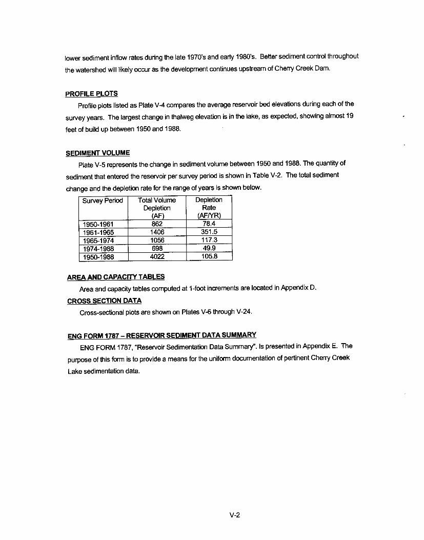
2001 ACE-OMAHA, TRI-LAKES SEDIMENT STUDIES
Plate V-1. “Cherry Creek Reservoir Sedimentation Ranges” shows the locations of range monuments.
Table V-2. Summarizes reservoir volume depletion according to survey period.
2002 URS, CHERRY CREEK RESERVOIR TO SCOTT ROAD MAJOR DRAINAGEWAY PLANNING STUDY
Table 5-1. “Geomorphic Characteristics” tabulates channel grade, average low-flow channel width, average low-flow channel depth, average bankfull channel width, and average bankfull channel depth.
Table 5-2. “Geomorphic Conditions by Reach” tabulates reach grade, channel conditions, bank erosion, dominant stream form and Rosgen classification.
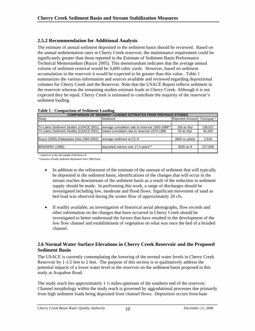
2006 TETRA TECH, DESIGN OF THE CHERRY CREEK SEDIMENT BASIN AND STABILIZATION MEASURES
Table 1. “Comparison of Sediment Loading” tabulates estimates of sediment loading rates Cherry Creek reservoir from previous completed studies, including USACE 2001, BRW-WRC 1985, and Ruzzo 2005.
2006 MULLER, CHERRY CREEK OPEN SPACE RESTORATION PROJECT
Sheet 2. “General Notes, Legend and Boring Logs” provides eight boring logs
Sheet 7. “Primary Channel Profile” shows existing and constructed channel profiles.
GK COTTON CONSULTING, INC. PAGE 24
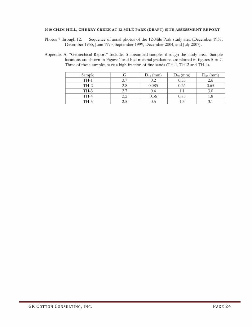
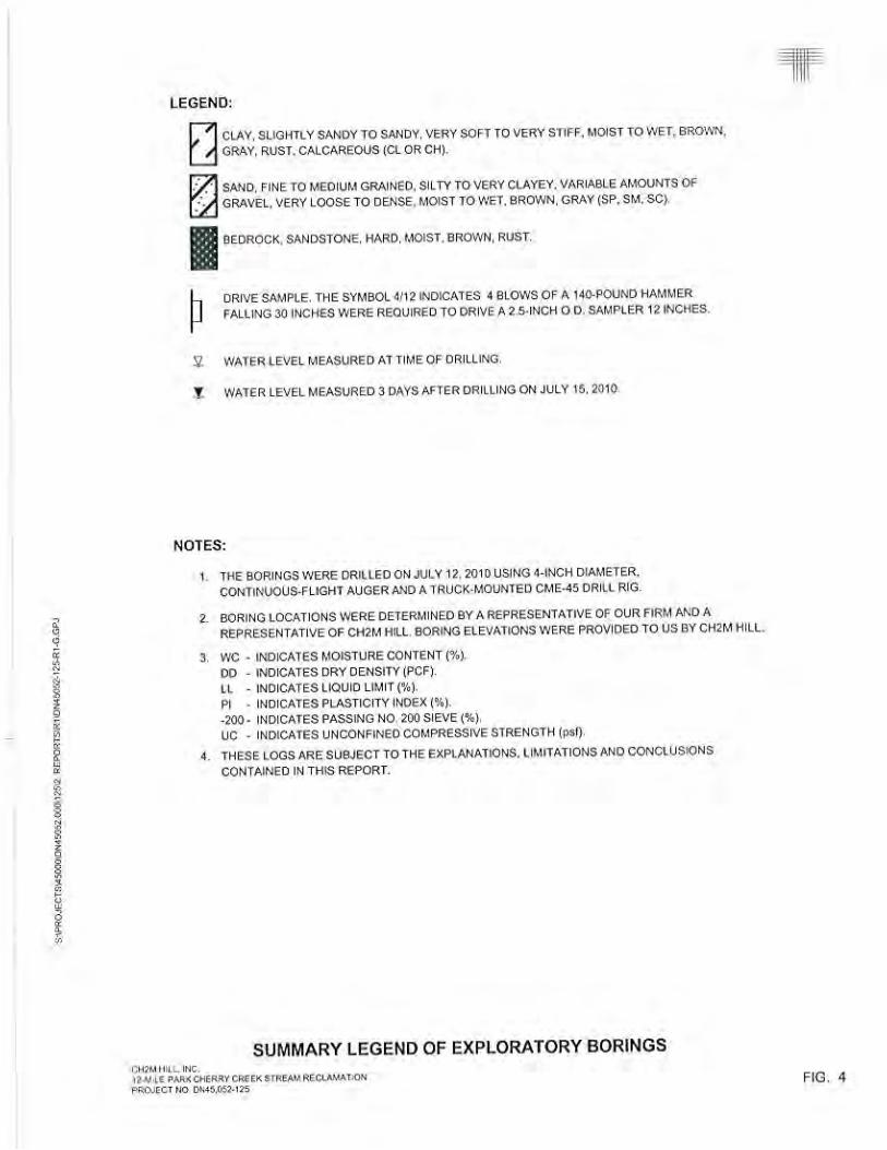
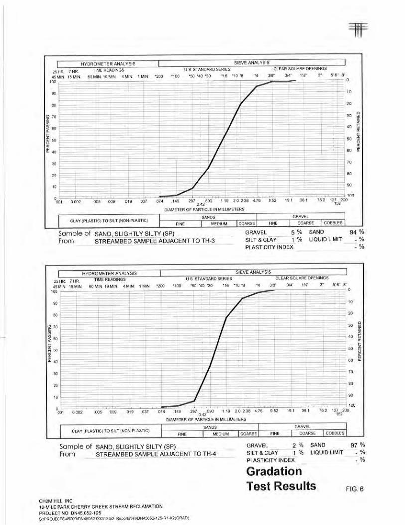
2010 CH2M HILL, CHERRY CREEK AT 12-MILE PARK (DRAFT) SITE ASSESSMENT REPORT
Photos 7 through 12. Sequence of aerial photos of the 12-Mile Park study area (December 1937, December 1955, June 1993, September 1999, December 2004, and July 2007).
Appendix A. “Geotechical Report” Includes 5 streambed samples through the study area. Sample locations are shown in Figure 1 and bed material gradations are plotted in figures 5 to 7. Three of these samples have a high fraction of fine sands (TH-1, TH-2 and TH-4).
Sample G D15 (mm) D50 (mm) D85 (mm) TH-1 3.7 0.2 0.55 2.6 TH-2 2.8 0.085 0.26 0.65 TH-3 2.7 0.4 1.1 3.0 TH-4 2.2 0.36 0.75 1.8 TH-5 2.5 0.5 1.3 3.1

GK COTTON CONSULTING, INC. PAGE 25
APPENDIX A. SITE PHOTOS AND LOCATION MAPS
Figure 16. Location of Sediment sampling sites 1, 2 and 3.

GK COTTON CONSULTING, INC. PAGE 26
Figure 17. Site #1 – Stream bed material sample in Cherry Creek State Park
Figure 18. Site #1 – Bank material sample (left bank)

GK COTTON CONSULTING, INC. PAGE 27
Figure 19. Site #2– Stream bed material sample near E. Caley Avenue at Valley Country Club
Figure 20. Site #3 – Stream bed material sample on Piney Creek at Fraser Street

GK COTTON CONSULTING, INC. PAGE 28
Figure 21. Location of Sediment sampling sites 4, 5, 6 and 7.

GK COTTON CONSULTING, INC. PAGE 29
Figure 22. Site #4 – Stream bed material sample at Broncos Parkway
Figure 23. Site #5 – Stream bed material sample at Cherry Creek Trail on Happy Canyon Creek

GK COTTON CONSULTING, INC. PAGE 30
Figure 24. Site #6 – Stream bed material sample near Tagawa Garden Center
Figure 25. Site #6 – Bank material sample near Tagawa Garden Center. Note that three strata have been exposed by recent lowering of the Cherry Creek channel. The upper layer was probably the stream bed prior to 2006, the center layer may be associated with the 1965 flood, and the lower strata are older valley sediments.
GK COTTON CONSULTING, INC. PAGE 31
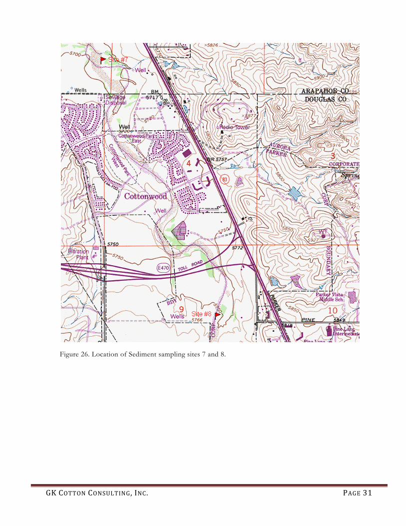
Figure 26. Location of Sediment sampling sites 7 and 8.

GK COTTON CONSULTING, INC. PAGE 32
Figure 27. Site #7 – Stream bed material sample upstream of Cherry Creek Trail drop structure (south boundary of Parker-Jordan Metro District property).
Figure 28. Site #8 – Stream bed material sample downstream of Pine Lane bridge

GK COTTON CONSULTING, INC. PAGE 33
APPENDIX B. CHANNEL SEDIMENT SAMPLES

Grain Size DistributionDescription: Cherry Creek Sedimentation Study, Gradation Testing
Sample Location: #1 - Bed Cherry CreekTesting by: Ground Engineering Consultants
Last revised:Printed:
Gradation Attributes:Gradation Coef, G = 2.3
d50 = 1.25 mm d90 = 3.67 mmd84.1 = 2.89 mm d65 = 1.72 mmd15.9 = 0.54 mm d02 = 0.22 mm
Sieve Size (opening)
Particle Size, d (mm)
Fraction Finer SNV
2.0 50.0 1.0001.5 37.5 1.0001.0 25.0 1.000
0.75 19.0 1.0000.50 12.5 1.000
0.375 9.5 1.000#4 4.75 0.940 1.555
#10 2.00 0.720 0.583#16 1.18 0.510 0.025#40 0.425 0.090 -1.341#50 0.300 0.030 -1.881
#100 0.150 0.010 -2.326#200 0.075 0.007 -2.457
16/Nov/201019/Nov/10 9:37
100.00Labeled0.01 0.002 -2.878 0.20.01 0.01 -2.326 1.00.01 0.02 -2.054 2.00.01 0.1 -1.282 10.00.01 0.2 -0.842 20.00.01 0.5 0.000 50.00.01 0.8 0.842 80.00.01 0.9 1.282 90.00.01 0.98 2.054 98.00.01 0.99 2.326 99.00.01 0.998 2.878 99.8
Unlabeled0.01 0.05 -1.645 1.10.01 0.15 -1.036 1.20.01 0.3 -0.524 1.40.01 0.4 -0.253 1.70.01 0.6 0.253 2.50.01 0.7 0.524 3.30.01 0.85 1.036 6.70.01 0.95 1.645 20.0
0.2 1 2 10 20 50 80 90 98 99 99.8
ds = 1.2456e0.8441 SNV
0.01
0.10
1.00
10.00
100.00
Particle Size, m
m
Finer (%)

Grain Size DistributionDescription: Cherry Creek Sedimentation Study, Gradation Testing
Sample Location: #1 - Bank Cherry CreekTesting by: Ground Engineering Consultants
Last revised:Printed:
Gradation Attributes:Gradation Coef, G = 27.8
d50 = 0.022 mmd84.1 = 0.62 mmd15.9 = 0.00 mm
Sieve Size (opening)
Particle Size, d (mm)
Fraction Finer SNV
2.0 50.0 1.0001.5 37.5 1.0001.0 25.0 1.000
0.75 19.0 0.940 1.555#4 4.75 0.930 1.476
#10 2.00 0.910 1.341#16 1.18 0.900 1.282#40 0.425 0.840 0.994#50 0.300 0.790 0.806
#100 0.150 0.700 0.524#200 0.075 0.632 0.337
16/Nov/201019/Nov/10 9:37
100.00Labeled0.01 0.002 -2.878 0.20.01 0.01 -2.326 1.00.01 0.02 -2.054 2.00.01 0.1 -1.282 10.00.01 0.2 -0.842 20.00.01 0.5 0.000 50.00.01 0.8 0.842 80.0
0.01 0.9 1.282 90.00.01 0.98 2.054 98.00.01 0.99 2.326 99.00.01 0.998 2.878 99.8
Unlabeled0.01 0.05 -1.645 1.10.01 0.15 -1.036 1.20.01 0.3 -0.524 1.40.01 0.4 -0.253 1.70.01 0.6 0.253 2.50.01 0.7 0.524 3.30.01 0.85 1.036 6.70.01 0.95 1.645 20.0
0.2 1 2 10 20 50 80 99 99.8
ds = 0.0218e3.3492 SNV
0.01
0.10
1.00
10.00
100.00
Particle Size, m
m
Finer (%)

Grain Size DistributionDescription: Cherry Creek Sedimentation Study, Gradation TestingTesting by: Ground Engineering Consultants
Sample Location: #2 - Bed Piney CreekLast revised:
Printed:
Gradation Attributes:Gradation Coef, G = 1.8
d50 = 0.93 mm d90 = 2.00 mmd84.1 = 1.69 mm d65 = 1.17 mmd15.9 = 0.51 mm d02 = 0.27 mm
Sieve Size (opening)
Particle Size, d (mm)
Fraction Finer SNV
2.0 50.0 1.0001.5 37.5 1.0001.0 25.0 1.000
0.75 19.0 1.0000.50 12.5 1.000
0.375 9.5 1.000#4 4.75 0.990 2.326
#10 2.00 0.930 1.476#16 1.18 0.780 0.772#40 0.425 0.090 -1.341#50 0.300 0.020 -2.054
#200 0.075 0.001 -3.090
Labeled
16/Nov/201019/Nov/10 9:37
100.000.01 0.002 -2.878 0.20.01 0.01 -2.326 1.00.01 0.02 -2.054 2.00.01 0.1 -1.282 10.00.01 0.2 -0.842 20.00.01 0.5 0.000 50.00.01 0.8 0.842 80.00.01 0.9 1.282 90.00.01 0.98 2.054 98.00.01 0.99 2.326 99.00.01 0.998 2.878 99.8
Unlabeled0.01 0.05 -1.645 1.10.01 0.15 -1.036 1.20.01 0.3 -0.524 1.40.01 0.4 -0.253 1.70.01 0.6 0.253 2.50.01 0.7 0.524 3.30.01 0.85 1.036 6.70.01 0.95 1.645 20.0
0.2 1 2 10 20 50 80 90 98 99 99.8
ds = 0.9329e0.5969 SNV
0.01
0.10
1.00
10.00
100.00
Particle Size, m
m
Finer (%)
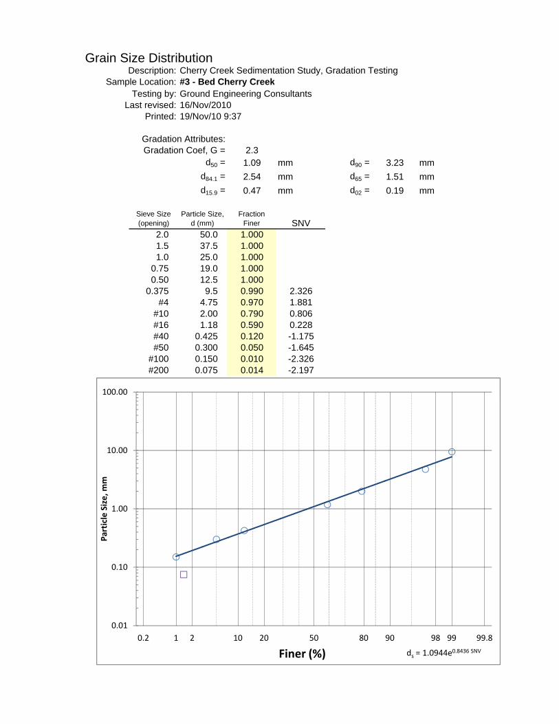
Grain Size DistributionDescription: Cherry Creek Sedimentation Study, Gradation Testing
Sample Location: #3 - Bed Cherry CreekTesting by: Ground Engineering Consultants
Last revised:Printed:
Gradation Attributes:Gradation Coef, G = 2.3
d50 = 1.09 mm d90 = 3.23 mmd84.1 = 2.54 mm d65 = 1.51 mmd15.9 = 0.47 mm d02 = 0.19 mm
Sieve Size (opening)
Particle Size, d (mm)
Fraction Finer SNV
2.0 50.0 1.0001.5 37.5 1.0001.0 25.0 1.000
0.75 19.0 1.0000.50 12.5 1.000
0.375 9.5 0.990 2.326#4 4.75 0.970 1.881
#10 2.00 0.790 0.806#16 1.18 0.590 0.228#40 0.425 0.120 -1.175#50 0.300 0.050 -1.645
#100 0.150 0.010 -2.326#200 0.075 0.014 -2.197
16/Nov/201019/Nov/10 9:37
100.00 Labeled0.01 0.002 -2.878 0.20.01 0.01 -2.326 1.00.01 0.02 -2.054 2.00.01 0.1 -1.282 10.00.01 0.2 -0.842 20.00.01 0.5 0.000 50.00.01 0.8 0.842 80.00.01 0.9 1.282 90.00.01 0.98 2.054 98.00.01 0.99 2.326 99.00.01 0.998 2.878 99.8
Unlabeled0.01 0.05 -1.645 1.10.01 0.15 -1.036 1.20.01 0.3 -0.524 1.40.01 0.4 -0.253 1.70.01 0.6 0.253 2.50.01 0.7 0.524 3.30.01 0.85 1.036 6.70.01 0.95 1.645 20.0
0.2 1 2 10 20 50 80 90 98 99 99.8
ds = 1.0944e0.8436 SNV
0.01
0.10
1.00
10.00
100.00
Particle Size, m
m
Finer (%)

Grain Size DistributionDescription: Cherry Creek Sedimentation Study, Gradation Testing
Sample Location: #4 - Bed Cherry CreekTesting by: Ground Engineering Consultants
Last revised:Printed:
Gradation Attributes:Gradation Coef, G = 2.2
d50 = 1.04 mm d90 = 2.91 mmd84.1 = 2.32 mm d65 = 1.42 mmd15.9 = 0.47 mm d02 = 0.20 mm
Sieve Size (opening)
Particle Size, d (mm)
Fraction Finer SNV
2.0 50.0 1.0001.5 37.5 1.0001.0 25.0 1.000
0.75 19.0 0.940 1.5550.50 12.5 0.890 1.227
0.375 9.5 0.850 1.036#4 4.75 0.690 0.496
#10 2.00 0.500 0.000#16 1.18 0.370 -0.332#40 0.425 0.140 -1.080#50 0.300 0.080 -1.405
#100 0.150 0.040 -1.751#200 0.075 0.032 -1.852
16/Nov/201019/Nov/10 9:37
100.00 Labeled0.01 0.002 -2.878 0.20.01 0.01 -2.326 1.00.01 0.02 -2.054 2.00.01 0.1 -1.282 10.00.01 0.2 -0.842 20.00.01 0.5 0.000 50.00.01 0.8 0.842 80.00.01 0.9 1.282 90.00.01 0.98 2.054 98.00.01 0.99 2.326 99.00.01 0.998 2.878 99.8
Unlabeled0.01 0.05 -1.645 1.10.01 0.15 -1.036 1.20.01 0.3 -0.524 1.40.01 0.4 -0.253 1.70.01 0.6 0.253 2.50.01 0.7 0.524 3.30.01 0.85 1.036 6.70.01 0.95 1.645 20.0
0.2 1 2 10 20 50 80 90 98 99 99.8
ds = 1.0425e0.8021 SNV
0.01
0.10
1.00
10.00
100.00
Particle Size, m
m
Finer (%)

Grain Size DistributionDescription: Cherry Creek Sedimentation Study, Gradation Testing
Sample Location: #5 - Happy Canyon CreekTesting by: Ground Engineering Consultants
Last revised:Printed:
Gradation Attributes:Gradation Coef, G = 2.1
d50 = 0.92 mm d90 = 2.35 mmd84.1 = 1.91 mm d65 = 1.22 mmd15.9 = 0.44 mm d02 = 0.20 mm
Sieve Size (opening)
Particle Size, d (mm)
Fraction Finer SNV
2.0 50.0 1.0001.5 37.5 1.0001.0 25.0 1.000
0.75 19.0 1.0000.50 12.5 1.000
0.375 9.5 1.000#4 4.75 0.990 2.326
#10 2.00 0.860 1.080#16 1.18 0.600 0.253#40 0.425 0.110 -1.227#50 0.300 0.040 -1.751
#100 0.150 0.020 -2.054#200 0.075 0.029 -1.896
16/Nov/201019/Nov/10 9:37
100.00 Labeled0.01 0.002 -2.878 0.20.01 0.01 -2.326 1.00.01 0.02 -2.054 2.00.01 0.1 -1.282 10.00.01 0.2 -0.842 20.00.01 0.5 0.000 50.00.01 0.8 0.842 80.00.01 0.9 1.282 90.00.01 0.98 2.054 98.00.01 0.99 2.326 99.00.01 0.998 2.878 99.8
Unlabeled0.01 0.05 -1.645 1.10.01 0.15 -1.036 1.20.01 0.3 -0.524 1.40.01 0.4 -0.253 1.70.01 0.6 0.253 2.50.01 0.7 0.524 3.30.01 0.85 1.036 6.70.01 0.95 1.645 20.0
0.2 1 2 10 20 50 80 90 98 99 99.8
ds = 0.9152e0.7354 SNV
0.01
0.10
1.00
10.00
100.00
Particle Size, m
m
Finer (%)

Grain Size DistributionDescription: Cherry Creek Sedimentation Study, Gradation Testing
Sample Location: #6 - Bed Cherry CreekTesting by:
Last revised:Printed:
Gradation Attributes:Gradation Coef, G = 2.2
d50 = 1.55 mm d90 = 4.18 mmd84.1 = 3.36 mm d65 = 2.09 mmd15.9 = 0.72 mm d02 = 0.32 mm
Sieve Size (opening)
Particle Size, d (mm)
Fraction Finer SNV
2.0 50.0 1.0001.5 37.5 1.0001.0 25.0 1.000
0.75 19.0 1.0000.50 12.5 1.000
0.375 9.5 1.000#4 4.75 0.930 1.476
#10 2.00 0.610 0.279#16 1.18 0.370 -0.332#40 0.425 0.040 -1.751#50 0.300 0.020 -2.054
#100 0.150 0.020 -2.054#200 0.075 0.012 -2.257
Ground Engineering Con16/Nov/201019/Nov/10 9:37
100.00 Labeled0.01 0.002 -2.878 0.20.01 0.01 -2.326 1.00.01 0.02 -2.054 2.00.01 0.1 -1.282 10.00.01 0.2 -0.842 20.00.01 0.5 0.000 50.00.01 0.8 0.842 80.00.01 0.9 1.282 90.00.01 0.98 2.054 98.00.01 0.99 2.326 99.00.01 0.998 2.878 99.8
Unlabeled0.01 0.05 -1.645 1.10.01 0.15 -1.036 1.20.01 0.3 -0.524 1.40.01 0.4 -0.253 1.70.01 0.6 0.253 2.50.01 0.7 0.524 3.30.01 0.85 1.036 6.70.01 0.95 1.645 20.0
0.2 1 2 10 20 50 80 90 98 99 99.8
ds = 1.5518e0.7726 SNV
0.01
0.10
1.00
10.00
100.00
Particle Size, m
m
Finer (%)

Grain Size DistributionDescription: Cherry Creek Sedimentation Study, Gradation Testing
Sample Location: #6 - Bank Cherry CreekTesting by: Ground Engineering Consultants
Last revised:Printed:
Gradation Attributes:Gradation Coef, G = 3.0
d50 = 0.96 mm d90 = 4.01 mmd84.1 = 2.92 mm d65 = 1.48 mmd15.9 = 0.32 mm d02 = 0.10 mm
Sieve Size (opening)
Particle Size, d (mm)
Fraction Finer SNV
2.0 50.0 1.0001.5 37.5 1.0001.0 25.0 1.000
0.75 19.0 1.0000.50 12.5 1.000
0.375 9.5 1.000#4 4.75 0.940 1.555
#10 2.00 0.700 0.524#16 1.18 0.530 0.075#40 0.425 0.240 -0.706#50 0.300 0.170 -0.954
#100 0.150 0.130 -1.126#200 0.075 0.118 -1.185
16/Nov/201019/Nov/10 9:37
100.00 Labeled0.01 0.002 -2.878 0.20.01 0.01 -2.326 1.00.01 0.02 -2.054 2.00.01 0.1 -1.282 10.00.01 0.2 -0.842 20.00.01 0.5 0.000 50.00.01 0.8 0.842 80.00.01 0.9 1.282 90.00.01 0.98 2.054 98.00.01 0.99 2.326 99.00.01 0.998 2.878 99.8
Unlabeled0.01 0.05 -1.645 1.10.01 0.15 -1.036 1.20.01 0.3 -0.524 1.40.01 0.4 -0.253 1.70.01 0.6 0.253 2.50.01 0.7 0.524 3.30.01 0.85 1.036 6.70.01 0.95 1.645 20.0
0.2 1 2 10 20 50 80 90 98 99 99.8
ds = 0.9622e1.1128 SNV
0.01
0.10
1.00
10.00
100.00
Particle Size, m
m
Finer (%)

Grain Size DistributionDescription: Cherry Creek Sedimentation Study, Gradation Testing
Sample Location: #7 - Bed Cherry CreekTesting by: Ground Engineering Consultants
Last revised:Printed:
Gradation Attributes:Gradation Coef, G = 3.4
d50 = 1.95 mm d90 = 9.35 mmd84.1 = 6.62 mm d65 = 3.13 mmd15.9 = 0.58 mm d02 = 0.16 mm
Sieve Size (opening)
Particle Size, d (mm)
Fraction Finer SNV
2.0 50.0 1.0001.5 37.5 1.0001.0 25.0 1.000
0.75 19.0 1.0000.50 12.5 1.000
0.375 9.5 0.990 2.326#4 4.75 0.770 0.739
#10 2.00 0.480 -0.050#16 1.18 0.360 -0.358#40 0.425 0.120 -1.175#50 0.300 0.050 -1.645
#100 0.150 0.020 -2.054#200 0.075 0.012 -2.257
16/Nov/201019/Nov/10 9:37
100.00 Labeled0.01 0.002 -2.878 0.20.01 0.01 -2.326 1.00.01 0.02 -2.054 2.00.01 0.1 -1.282 10.00.01 0.2 -0.842 20.00.01 0.5 0.000 50.00.01 0.8 0.842 80.00.01 0.9 1.282 90.00.01 0.98 2.054 98.00.01 0.99 2.326 99.00.01 0.998 2.878 99.8
Unlabeled0.01 0.05 -1.645 1.10.01 0.15 -1.036 1.20.01 0.3 -0.524 1.40.01 0.4 -0.253 1.70.01 0.6 0.253 2.50.01 0.7 0.524 3.30.01 0.85 1.036 6.70.01 0.95 1.645 20.0
0.2 1 2 10 20 50 80 90 98 99 99.8
ds = 1.9523e1.2224 SNV
0.01
0.10
1.00
10.00
100.00
Particle Size, m
m
Finer (%)

Grain Size DistributionDescription: Cherry Creek Sedimentation Study, Gradation Testing
Sample Location: #7 - Bed Cherry CreekTesting by: Ground Engineering Consultants
Last revised:Printed:
Gradation Attributes:Gradation Coef, G = 3.1
d50 = 1.90 mm d90 = 8.10 mmd84.1 = 5.88 mm d65 = 2.94 mmd15.9 = 0.61 mm d02 = 0.19 mm
Sieve Size (opening)
Particle Size, d (mm)
Fraction Finer SNV
2.0 50.0 1.0001.5 37.5 1.0001.0 25.0 1.000
0.75 19.0 1.0000.50 12.5 1.000
0.375 9.5 0.980 2.054#4 4.75 0.780 0.772
#10 2.00 0.490 -0.025#16 1.18 0.360 -0.358#40 0.425 0.120 -1.175#50 0.300 0.050 -1.645
#100 0.150 0.010 -2.326#200 0.075 0.007 -2.457
16/Nov/201019/Nov/10 9:37
100.00 Labeled0.01 0.002 -2.878 0.20.01 0.01 -2.326 1.00.01 0.02 -2.054 2.00.01 0.1 -1.282 10.00.01 0.2 -0.842 20.00.01 0.5 0.000 50.00.01 0.8 0.842 80.00.01 0.9 1.282 90.00.01 0.98 2.054 98.00.01 0.99 2.326 99.00.01 0.998 2.878 99.8
Unlabeled0.01 0.05 -1.645 1.10.01 0.15 -1.036 1.20.01 0.3 -0.524 1.40.01 0.4 -0.253 1.70.01 0.6 0.253 2.50.01 0.7 0.524 3.30.01 0.85 1.036 6.70.01 0.95 1.645 20.0
0.2 1 2 10 20 50 80 90 98 99 99.8
ds = 1.8987e1.1323 SNV
0.01
0.10
1.00
10.00
100.00
Particle Size, m
m
Finer (%)

GK COTTON CONSULTING, INC. PAGE 44
APPENDIX C . EXTRACTS FROM OTHER STUDIES
Pages from 1985_BRW-WRC “Feasibility study for the Cherry Creek Basin drainageway” ................ 45
Pages from 2001_ACE-Omaha District “TriLakes sediment studies” ..................................................... 48
Pages from 2002_URS “Cherry Creek Reservoir_to_Scott Road - MDP” .............................................. 50
Pages from 2006_MULLER “Cherry Creek Open Space Restoration Project-As-builts” .................... 53
Pages from 2006_TETRA TECH “Design of the Cherry Creek sediment basin and stabilization measures”................................................................................................................................................ 55
Pages from 2010_CH2M HILL “DRAFT Cherry Creek 12 Mile Site Assessment_v5-WPR”............. 56


Cherry Creek Sediment Basin and Stream Stabilization Measures
Cherry Creek Basin Water Quality Authority December 11, 2006
10
2.5.2 Recommendation for Additional Analysis The estimate of annual sediment deposited in the sediment basin should be reviewed. Based on the annual sedimentation rates in Cherry Creek reservoir, the maintenance requirement could be significantly greater than those reported in the Estimate of Sediment Basin Performance Technical Memorandum (Ruzzo 2005). This memorandum indicates that the average annual volume of sediment removal would be 3,600 cubic yards. However, based on sediment accumulation in the reservoir it would be expected to be greater than this value. Table 1 summarizes the various information and sources available and reviewed regarding depositional volumes for Cherry Creek and the Reservoir. Note that the USACE Report reflects sediment in the reservoir whereas the remaining studies estimate loads in Cherry Creek. Although it is not expected they be equal, Cherry Creek is estimated to contribute the majority of the reservoir’s sediment loading. Table 1 - Comparison of Sediment Loading
Study Sediment Reported Amount Tons/year *
Tri-Lakes Sediment Studies (USACE 2001) average cumulation rate to reservoir 1950-1988** 106 ac-ft/yr 138,521Tri-Lakes Sediment Studies (USACE 2001) lowest cumulation rate to reservoir 1974-1988 50 ac-ft/yr 65,340
Ruzzo (2005) (Halepaska Data 1984-2002) average sediment at CC-8 3600 cu yds/yr 2,916
BRW/WRC (1985) deposited volume over 17.4 years** 3035 ac-ft 227,939
* based on a dry unit weight of 60 lbs/cu ft**volumes include sediment deposition from 1965 flood
COMPARISON OF SEDIMENT LOADING ESTIMATES FROM PREVIOUS STUDIES
• In addition to the refinement of the estimate of the amount of sediment that will typically be deposited in the sediment basin, identifications of the changes that will occur in the stream reaches downstream of the sediment basin as a result of the reduction in sediment supply should be made. In performing this work, a range of discharges should be investigated including low, moderate and flood flows. Significant movement of sand as bed load was observed during the winter flow of approximately 20 cfs.
• If readily available, an investigation of historical aerial photographs, flow records and
other information on the changes that have occurred in Cherry Creek should be investigated to better understand the factors that have resulted in the development of the low flow channel and establishment of vegetation on what was once the bed of a braided channel.
2.6 Normal Water Surface Elevations in Cherry Creek Reservoir and the Proposed Sediment Basin The USACE is currently contemplating the lowering of the normal water levels in Cherry Creek Reservoir by 1-1/2 feet to 2 feet. The purpose of this section is to qualitatively address the potential impacts of a lower water level in the reservoir on the sediment basin proposed in this study at Arapahoe Road. The study reach lies approximately 1 ½ miles upstream of the southern end of the reservoir. Channel morphology within the study reach is governed by aggradational processes due primarily from high sediment loads being deposited from channel flows. Deposition occurs from base

24
appear until the 1993 aerial photos. This suggests that this area is a result of elevated ground water caused by the reservoir.
Based on the available historic aerial imagery, the existing channel appears to be very stable. The channel is not actively moving outside of the historic flow path over time. The most significant geomorphic event to occur in the channel corridor is the construction of the Reservoir resulting in an elevated water table. This has resulted in overbank ponds and groundwater fed secondary channels forming through the project area. This has also created a vibrant riparian habitat with multiple areas of wetland vegetation. Aerial images are provided below for the project area.
Photo 7 - Aerial Photo 1, December 1937

25
Photo 8 - Aerial Photo 2, December 1955

26
Photo 9 - Aerial Photo 3, June 1993

27
Photo 10 - Aerial Photo 4, September 1999

28
Photo 11 - Aerial Photo 5, December 2004

29
Photo 12 - Aerial Image 6, July 2007


GEORGE K COTTON CONSULTING, INC Hydrologic Engineering and Design
Design Flows in the Cherry Creek 1 | P a g e
MEMORANDUM
To: Molly Trujillo, PE
From: George Cotton, PE
Date: March 11, 2011
Subject: Design Flows in the Cherry Creek
The purpose of this memo is to evaluate long-term hydrology of the Cherry Creek in the sedimentation study reach (Pine Lane to the Reservoir). This is a losing reach, according to models that take into consideration water supply operations. It is likely that water diversion from the alluvial aquifer affects flood hydrology and channel forming discharges. Three hydrology studies are reviewed: the SMWSA Master Plan, the Major Drainageway Planning Study, and the CCBWQA phosphorus model.
Analysis of SMWSA Master Plan In 2007, the South Metro Water Supply Authority published its master plan for water
supply development. SMWSA is an umbrella for 13 water providers, most of which are within the Cherry Creek basin. More than 80% of the SMWSA water supply is used within the Cherry Creek basin. Future storage of renewable water supplies by all of the SMWSA water providers occurs at the new Rueter-Hess reservoir, which is also within the Cherry Creek basin.
Figure 2-3 (below) from the SMWSA Master Plan shows the breakdown of water supplies over the planning horizon. Table 1 provides the same information as the graph and also back casts to the year 2000.
Figure 1. Taken from SMWSA Master Plan 2007

GEORGE K COTTON CONSULTING, INC Hydrologic Engineering and Design
Design Flows in the Cherry Creek 2 | P a g e
Table 1. SMWSA Water Sources over planning horizon
Year Renewable Supply
Surface Supply
Renewable Buffer
Ground Water
Recap / Return
Alluvial (water rights)
Total
2000 0 500 0 42220 3000 3500 49220 2010 4000 24300 400 25900 11900 4300 708002020 17800 27100 1780 19800 20800 5100 923802030 32900 25100 3290 14900 24000 5100 105290
Buildout 43400 25100 4340 14900 28100 5100 120940
Most of the water supply for the SMWSA water providers comes from imported sources. SMWSA’s goal is to shift from a heavy dependence on non-renewable groundwater to renewable water supplies by acquiring surface water rights in other basins and transporting this supply to the SMWSA service area and then to each service provider. This will require the development of existing water rights (called surface supply), then acquiring and developing new water rights (called renewable supply). This will permit ground water use to decline. To account for uncertainty in this process, the master plan includes a renewable buffer that is equal to 10% of the estimated required renewable supply.
A second source of water supply for SMWSA water providers comes from the recapture of flows or return flows. These flows will largely be recovered through alluvial wells. Also, most of the surface water rights on Cherry Creek are diverted through alluvial wells.
So, water supply for SMWSA water providers can be aggregated into two classes: imported supplies (renewable, surface, and groundwater), and alluvial (recapture / return and alluvial water rights). I estimate that on an annual basis about 44% of the total supply will be returned (assuming that 42% of the supply is for domestic use and 58% is for irrigation, with 10% consumption of domestic water and 90% consumption of irrigation). Table 2 provides an estimate of the un-diverted alluvial flow (both flow in the alluvial aquifers and in surface streams), where the un-diverted alluvial flow is equal to 44% of the total supply minus the diverted alluvial flow. These data are shown graphically in Figure 2.
Table 2. Estimate of Un-Diverted Alluvial Flows within SMWSA
Year Total Diverted Alluvial
Imported Flows
Un‐Diverted Alluvial
2000 49220 6500 42720 149602010 70800 16200 54600 146692020 92380 25900 66480 143782030 105290 29100 76190 16806
Buildout 120940 33200 87740 19530 In 2000, 82% of the SMWSA water providers were associated with the Cherry Creek
basin. Using sub-reach 880 in the CCBWQA model (Parker, CO) as a point of reference the SMWSA master plan estimates that 12,300 ac-ft of un-diverted alluvial flow occurred at this point in the Cherry Creek. This compares with 11,700 ac-ft estimated by the CCBWQA model. In addition, the CCBWQA model estimates a reach flow loss of 2,500 ac-ft compared to SMWSA estimate of 5,300 ac-ft.

GEORGE K COTTON CONSULTING, INC Hydrologic Engineering and Design
Design Flows in the Cherry Creek 3 | P a g e
Figure 2. SMWSA Master Plan Water Supply Breakdown
Recovery of flows will increase steadily, which will increase the total diverted alluvial flow in the Cherry Creek. In 2000, only about 6.1% of the total supply was recovered. SMWSA estimates that in 2010, 16.8% was recovered and that by 2020 22.5% will be recovered, which will be close to the maximum expected recovery that will be achieved at build out (23.2%). The result is that un-diverted alluvial flows remain essentially unchanged even as water supply is dramatically increased to the Cherry Creek basin. Of all of the sources of water supply for water providers in SMWSA, recovered flows are probably one of the least difficult to acquire administratively and the least costly to deliver.
Analysis of Major Drainageway Master Plan The “Cherry Creek Major Drainageway Planning Study” was prepared in 2002 and
provides an estimate of the flood hydrology for existing and future conditions in the basin. This hydrology deals directly with the main effect of rural to urban land use change, which is the increase in impervious area and the resulting increase in runoff volume. This is a condition that is not addressed by the SMWSA master plan for the reason that stormwater runoff is considered a minor and unreliable source of water. This may not be entirely true. From 1985 to 2010, basin imperviousness has increased for 13% to 23% and will continue to increase at the rate of 1% for every 11,600 housing units built in the basin. Runoff from these impervious areas ultimately connects to the Cherry Creek, where it may be diverted for water supply as long as overall basin yield from Cherry Creek tends to maintain the historical average.
Urban runoff enters the Cherry Creek via storm drainage outfalls and tributary drainageways. It appears that alluvial pumping very quickly captures minor runoff. So CCBWQA estimates of base flow, which comport with SMWSA planning, indicate that the “Cherry Creek Major Drainageway Planning Study” probably over estimates frequent floods such as the 2-year.
GEORGE K COTTON CONSULTING, INC Hydrologic Engineering and Design
Design Flows in the Cherry Creek 4 | P a g e
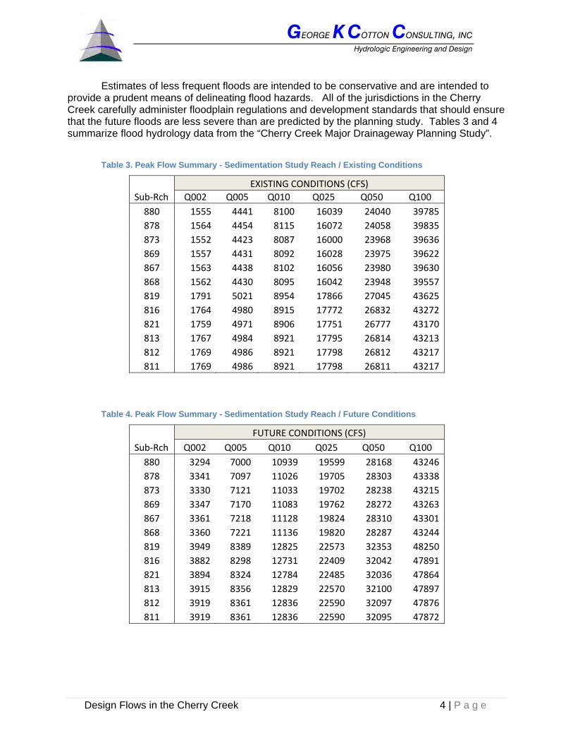
Estimates of less frequent floods are intended to be conservative and are intended to provide a prudent means of delineating flood hazards. All of the jurisdictions in the Cherry Creek carefully administer floodplain regulations and development standards that should ensure that the future floods are less severe than are predicted by the planning study. Tables 3 and 4 summarize flood hydrology data from the “Cherry Creek Major Drainageway Planning Study”.
Table 3. Peak Flow Summary - Sedimentation Study Reach / Existing Conditions
EXISTING CONDITIONS (CFS) Sub‐Rch Q002 Q005 Q010 Q025 Q050 Q100 880 1555 4441 8100 16039 24040 39785 878 1564 4454 8115 16072 24058 39835 873 1552 4423 8087 16000 23968 39636 869 1557 4431 8092 16028 23975 39622 867 1563 4438 8102 16056 23980 39630 868 1562 4430 8095 16042 23948 39557 819 1791 5021 8954 17866 27045 43625 816 1764 4980 8915 17772 26832 43272 821 1759 4971 8906 17751 26777 43170 813 1767 4984 8921 17795 26814 43213 812 1769 4986 8921 17798 26812 43217 811 1769 4986 8921 17798 26811 43217
Table 4. Peak Flow Summary - Sedimentation Study Reach / Future Conditions
FUTURE CONDITIONS (CFS) Sub‐Rch Q002 Q005 Q010 Q025 Q050 Q100 880 3294 7000 10939 19599 28168 43246 878 3341 7097 11026 19705 28303 43338 873 3330 7121 11033 19702 28238 43215 869 3347 7170 11083 19762 28272 43263 867 3361 7218 11128 19824 28310 43301 868 3360 7221 11136 19820 28287 43244 819 3949 8389 12825 22573 32353 48250 816 3882 8298 12731 22409 32042 47891 821 3894 8324 12784 22485 32036 47864 813 3915 8356 12829 22570 32100 47897 812 3919 8361 12836 22590 32097 47876 811 3919 8361 12836 22590 32095 47872

GEORGE K COTTON CONSULTING, INC Hydrologic Engineering and Design
Design Flows in the Cherry Creek 5 | P a g e
One approach to using the planning study flood hydrology would be to scale the existing 2-year flood peaks for sub-reaches by flow volume ratios (sub-reach volume divided by sub-reach 880 volume) as computed by the CCBWQA model (see Table 5). Using this approach, the 2-year existing and future conditions would be as shown in Table 6.
Table 5. Sub-Reach Flow Scaling following based on volume (CCBWQA model)
Sub-Reach 880 878 873 869 867 868 Volume (ac-ft) 76,368 74,567 72,358 67,681 65,061 65,718Flow Scaling 100.0% 97.6% 94.7% 88.6% 85.2% 86.1%
Sub-Reach 819 816 821 813 812 811 Volume (ac-ft) 70,918 61,328 62,880 59,287 56,555 52,232Flow Scaling 92.9% 80.3% 82.3% 77.6% 74.1% 68.4%
Table 6. “Cherry Creek Major Drainageway Planning Study” Scaled 2-year flows
Scaling Existing Conditions Future Conditions Sub‐Rch Factor Original Scaled Ratio Original Scaled Ratio
880 100.0% 1555 1555 100.0% 3294 3294 100.0%878 97.6% 1564 1518 97.0% 3341 3215 96.2%873 94.7% 1552 1473 94.9% 3330 3119 93.7%869 88.6% 1557 1378 88.5% 3347 2918 87.2%867 85.2% 1563 1325 84.8% 3361 2806 83.5%868 86.1% 1562 1339 85.7% 3360 2836 84.4%819 92.9% 1791 1445 80.7% 3949 3060 77.5%816 80.3% 1764 1249 70.8% 3882 2645 68.1%821 82.3% 1759 1280 72.8% 3894 2711 69.6%813 77.6% 1767 1207 68.3% 3915 2556 65.3%812 74.1% 1769 1152 65.1% 3919 2441 62.3%811 68.4% 1769 1064 60.1% 3919 2253 57.5%

GEORGE K COTTON CONSULTING, INC Hydrologic Engineering and Design
Design Flows in the Cherry Creek 6 | P a g e
CCBWQA Dominant Discharge The dominant discharge for a stream reach is the product of the probability of a stream
discharge multiplied by the sediment load in the reach. This probability approach places a higher weighting on frequent stream flows and lower weighting of rare stream flows. The discharge associated with the maximum weighted sediment loading is referred to as the dominant discharge. This method was used to identify the dominant discharge in the sub-reaches of the study reach over the eight year CCBWQA model simulation. Figure 3 shows the calculation results graphically.
Table 7. Sub-Reach dominant discharges (CCBWQA model)
Sub-Reach 880 878 873 869 867 868 Dominant Q (ac-ft/mo) 1080 880 960 550 500 800
Sub-Reach 819 816 821 813 812 811 Dominant Q (ac-ft/mo) 550 550 500 600 500 n/c
The weighting of more frequent sediment loads follows a normal pattern, which rises
steadily to a peak value. While there is a distinct peak in weighted sediment loads for each sub-reach, the less frequent sediment loads don’t decline and can reach values that equal or exceed the first peak. This may be a product of the short period of simulation or the complex way that water is routed and diverted from the Cherry Creek.
Recommended Flows While scaling of flows based on volume is admittedly a very approximate approach it has
the advantage of comporting to major drainageway planning and to the losing nature of reach as shown in the CCBWQA model and SMWSA master planning. In the long run, we recommend that the UDSWM model that was used for major drainageway planning be converted to EPA-SWMM. In this way, additional modeling elements found in the CCBWQA modeling elements could be included. EPA-SWMM has similar routines to those developed for the CCBWQA model (for example, alluvial groundwater flow simulation), so the conversion could draw on data and calibration work already conducted by CCBWQA.
For the time being, using scaled 2-year existing-conditions flows from the major drainageway planning study is recommended (green highlighted column in Table 6). Use of future flows is not recommended because the SMWSA planning does not show a future increase in un-diverted alluvial flows.
References Brown and Caldwell, 2008, “Cherry Creek Basin Watershed Phosphorus Model Documentation”
prepared for the Cherry Creek Basin Water Quality Authority
CDM, 2007, “South Metro Water Supply Authority Regional Water Master Plan” prepared for South Metro Water Supply Authority
URS, 2002, “Cherry Creek Corridor – Reservoir to Scott Road / Major Drainageway Planning Study” prepared for Arapahoe County, Douglas County, City of Aurora, City of Centennial, Town of Parker, Urban Drainage and Flood Control District

GEORGE K COTTON CONSULTING, INC Hydrologic Engineering and Design
Design Flows in the Cherry Creek 7 | P a g e
Figure 3 Shows plots of dominant discharge calculation as computed by sub-reach for the CCBWQA simulation. The vertical lines show the approximate location of the first peak in weighted sediment loading, i.e. the dominant discharge for the sub-reach (ac-ft/month). The vertical axis is the probability weighted sediment transport in tons.

GEORGE K COTTON CONSULTING, INC Hydrologic Engineering and Design
Engelund-Hansen Regression Equation 1 | P a g e
MEMORANDUM
To: Molly Trujillo, PE
From: George Cotton
Date: December 20, 2010
Subject: Regression form of the Engelund and Hansen Sediment Transport Capacity Approach
Engelund and Hansen’s Approach Engelund and Hansen (1967) proposed a method for determining total sediment load in
streams with dune-covered beds. The relationships are as follows:
f 0.1 θ . ................................................................................ Equation 1.0.0
:
S ......................................................................... Equation 1.1.0
f UU
.................................................................................... Equation 1.2.0
UU
0.6 2.5 ln .................................................. Equation 1.2.1
where: k 2.5 d
y y ....................................................................... Equation 1.3.1
θ .............................................................................. Equation 1.3.2
θ 0.06 0.4 θ ...................................................... Equation 1.3.2
With the value of y’o the mean velocity, U, can be calculated. The sediment load can then be expressed as:
g 0.05 U S
/ ............................................... Equation 2.0.0
Variable definitions and the associated units are provided in Appendix A.
Engelund (1973) also proposed a method for calculation of sediment transport when the bed material is graded. It assumed that particles finer than a certain size will all enter into suspension while larger grains will move as bed load. The criterion for critical size is based on the empirical value of 2.5 2.
GEORGE K COTTON CONSULTING, INC Hydrologic Engineering and Design
Engelund-Hansen Regression Equation 2 | P a g e
E-H Sediment transport capacity from HEC-RAS 4 While the Engelund and Hansen is not a particularly complex sediment transport
formula, there are several aspects of the approach that require detailed knowledge to implement in HEC-RAS 4. So as not to presume the approach taken by HEC, a set of sediment transport data was generated directly from HEC-RAS 4.
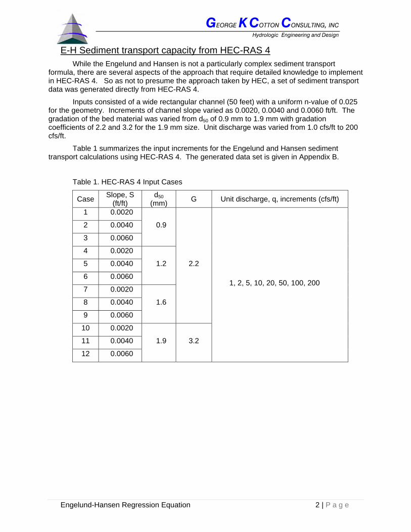
Inputs consisted of a wide rectangular channel (50 feet) with a uniform n-value of 0.025 for the geometry. Increments of channel slope varied as 0.0020, 0.0040 and 0.0060 ft/ft. The gradation of the bed material was varied from d50 of 0.9 mm to 1.9 mm with gradation coefficients of 2.2 and 3.2 for the 1.9 mm size. Unit discharge was varied from 1.0 cfs/ft to 200 cfs/ft.
Table 1 summarizes the input increments for the Engelund and Hansen sediment transport calculations using HEC-RAS 4. The generated data set is given in Appendix B.
Table 1. HEC-RAS 4 Input Cases
Case Slope, S (ft/ft)
d50 (mm) G Unit discharge, q, increments (cfs/ft)
1 0.0020
0.9
2.2
1, 2, 5, 10, 20, 50, 100, 200
2 0.0040
3 0.0060
4 0.0020
1.2 5 0.0040
6 0.0060
7 0.0020
1.6 8 0.0040
9 0.0060
10 0.0020
1.9 3.2 11 0.0040
12 0.0060
GEORGE K COTTON CONSULTING, INC Hydrologic Engineering and Design
Engelund-Hansen Regression Equation 3 | P a g e
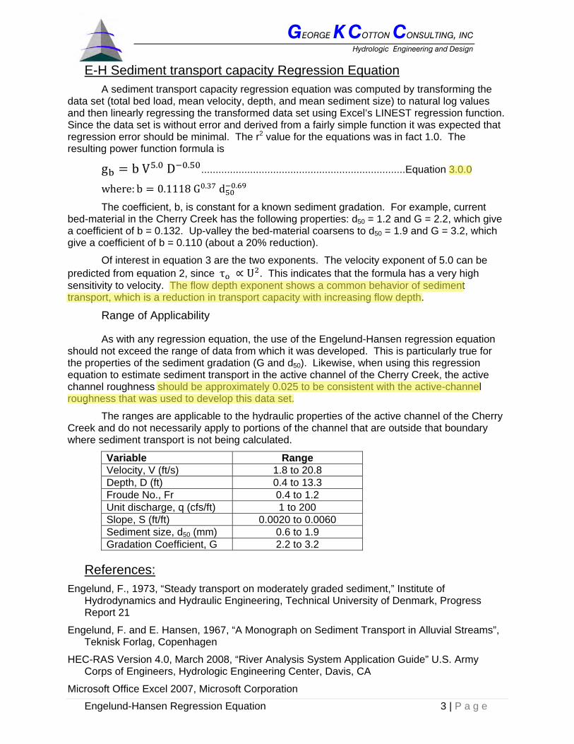
E-H Sediment transport capacity Regression Equation A sediment transport capacity regression equation was computed by transforming the
data set (total bed load, mean velocity, depth, and mean sediment size) to natural log values and then linearly regressing the transformed data set using Excel’s LINEST regression function. Since the data set is without error and derived from a fairly simple function it was expected that regression error should be minimal. The r2 value for the equations was in fact 1.0. The resulting power function formula is
g b V . D . ....................................................................... Equation 3.0.0
where: b 0.1118 G . d . The coefficient, b, is constant for a known sediment gradation. For example, current
bed-material in the Cherry Creek has the following properties: d50 = 1.2 and G = 2.2, which give a coefficient of b = 0.132. Up-valley the bed-material coarsens to d50 = 1.9 and G = 3.2, which give a coefficient of b = 0.110 (about a 20% reduction).
Of interest in equation 3 are the two exponents. The velocity exponent of 5.0 can be predicted from equation 2, since τ U . This indicates that the formula has a very high sensitivity to velocity. The flow depth exponent shows a common behavior of sediment transport, which is a reduction in transport capacity with increasing flow depth.
Range of Applicability
As with any regression equation, the use of the Engelund-Hansen regression equation should not exceed the range of data from which it was developed. This is particularly true for the properties of the sediment gradation (G and d50). Likewise, when using this regression equation to estimate sediment transport in the active channel of the Cherry Creek, the active channel roughness should be approximately 0.025 to be consistent with the active-channel roughness that was used to develop this data set.
The ranges are applicable to the hydraulic properties of the active channel of the Cherry Creek and do not necessarily apply to portions of the channel that are outside that boundary where sediment transport is not being calculated.
Variable Range Velocity, V (ft/s) 1.8 to 20.8 Depth, D (ft) 0.4 to 13.3 Froude No., Fr 0.4 to 1.2 Unit discharge, q (cfs/ft) 1 to 200 Slope, S (ft/ft) 0.0020 to 0.0060 Sediment size, d50 (mm) 0.6 to 1.9 Gradation Coefficient, G 2.2 to 3.2
References: Engelund, F., 1973, “Steady transport on moderately graded sediment,” Institute of
Hydrodynamics and Hydraulic Engineering, Technical University of Denmark, Progress Report 21
Engelund, F. and E. Hansen, 1967, “A Monograph on Sediment Transport in Alluvial Streams”, Teknisk Forlag, Copenhagen
HEC-RAS Version 4.0, March 2008, “River Analysis System Application Guide” U.S. Army Corps of Engineers, Hydrologic Engineering Center, Davis, CA
Microsoft Office Excel 2007, Microsoft Corporation
GEORGE K COTTON CONSULTING, INC Hydrologic Engineering and Design
Engelund-Hansen Regression Equation 4 | P a g e
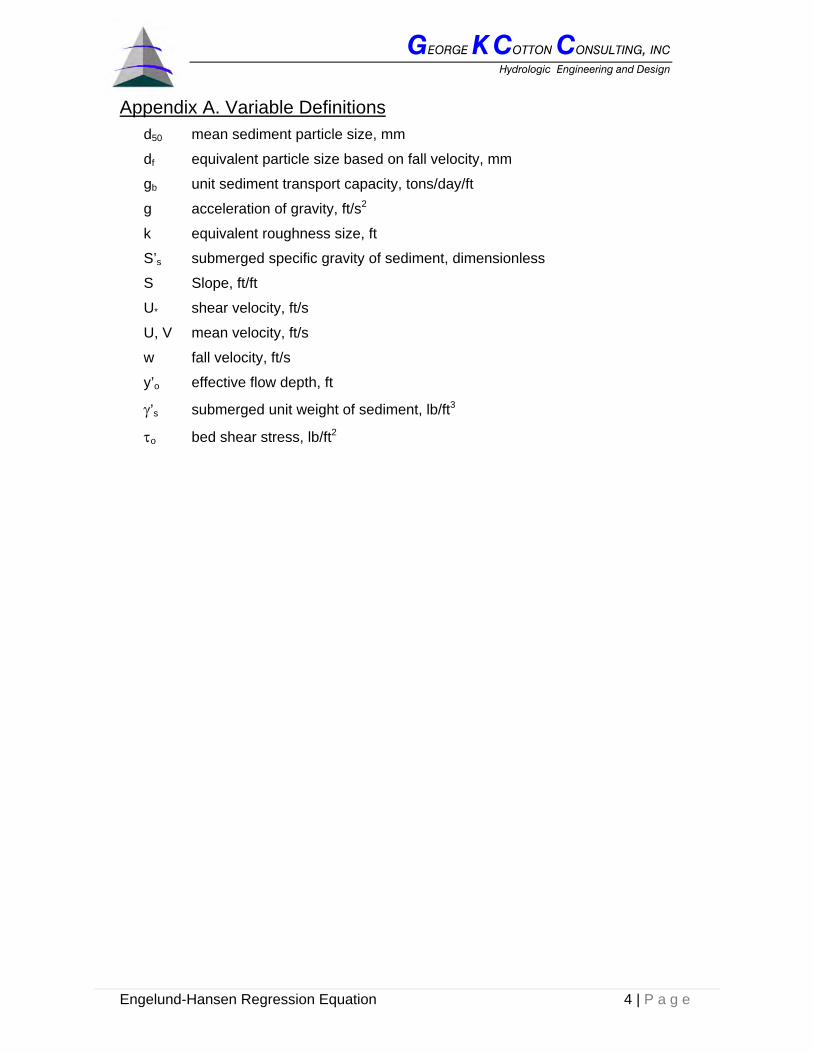
Appendix A. Variable Definitions d50 mean sediment particle size, mm
df equivalent particle size based on fall velocity, mm
gb unit sediment transport capacity, tons/day/ft
g acceleration of gravity, ft/s2
k equivalent roughness size, ft
S’s submerged specific gravity of sediment, dimensionless
S Slope, ft/ft
U* shear velocity, ft/s
U, V mean velocity, ft/s
w fall velocity, ft/s
y’o effective flow depth, ft
γ’s submerged unit weight of sediment, lb/ft3
τo bed shear stress, lb/ft2

GEORGE K COTTON CONSULTING, INC Hydrologic Engineering and Design
Engelund-Hansen Regression Equation 5 | P a g e
Appendix B. HEC-RAS 4 Data Set
Case G d50
(mm) S
(ft/ft) q
(cfs/ft) gb
(tons/day/ft)
V (ft/s)
D (ft)
1 2.2 0.6 0.002
1 5.3 1.8 0.56 2 17.3 2.37 0.84 5 82.1 3.42 1.46
10 267.0 4.51 2.21 20 868.4 5.96 3.35 50 4118 8.59 5.81
100 13350 11.33 8.8 200 43320 14.95 13.34
2 2.2 1.2 0.002
1 3.3 1.8 0.56 2 10.8 2.37 0.84 5 51.3 3.42 1.46
10 166.8 4.51 2.21 20 542.6 5.96 3.35 50 2574 8.59 5.81
100 8344 11.33 8.8 200 27060 14.95 13.34
3 2.2 1.6 0.002
1 2.7 1.8 0.56 2 8.7 2.37 0.84 5 41.4 3.42 1.46
10 134.6 4.51 2.21 20 438 5.96 3.35 50 2076 8.59 5.81
100 6734 11.33 8.8 200 21840 14.95 13.34
4 2.2 0.6 0.004
1 16.9 2.21 0.45 2 54.7 2.92 0.69 5 258.8 4.21 1.19
10 839 5.56 1.8 20 2724 7.33 2.73 50 12928 10.58 4.72
100 41940 13.96 7.15 200 136240 18.41 10.83
5 2.2 1.2 0.004
1 10.6 2.21 0.45 2 34.2 2.92 0.69 5 161.7 4.21 1.19
10 524.2 5.56 1.8 20 1702.2 7.33 2.73 50 8080 10.58 4.72
100 26200 13.96 7.15 200 85140 18.41 10.83

GEORGE K COTTON CONSULTING, INC Hydrologic Engineering and Design
Engelund-Hansen Regression Equation 6 | P a g e
(continued)
Case G d50
(mm) S
(ft/ft) q
(cfs/ft) gb
(tons/day/ft)
V (ft/s)
D (ft)
6 2.2 1.6 0.004
1 8.5 2.21 0.45 2 27.6 2.92 0.69 5 130.5 4.21 1.19
10 423.2 5.56 1.8 20 1373.8 7.33 2.73 50 6520 10.58 4.72
100 21160 13.96 7.15 200 68720 18.41 10.83
7 2.2 0.6 0.006
1 33.2 2.5 0.4 2 103.6 3.3 0.61 5 503 4.76 1.05
10 1638.8 6.28 1.59 20 5318 8.28 2.41 50 25240 11.95 4.18
100 81880 15.71 6.35 200 266000 20.78 9.6
8 2.2 1.2 0.006
1 20.7 2.5 0.4 2 64.8 3.3 0.61 5 314.4 4.76 1.05
10 1024.2 6.28 1.59 20 3324 8.28 2.41 50 15772 11.95 4.18
100 51180 15.71 6.35 200 166240 20.78 9.6
9 2.2 1.6 0.006
1 16.7 2.5 0.4 2 52.3 3.3 0.61 5 253.8 4.76 1.05
10 826.6 6.28 1.59 20 2682 8.28 2.41 50 12730 11.95 4.18
100 41300 15.71 6.35 200 134180 20.78 9.6

GEORGE K COTTON CONSULTING, INC Hydrologic Engineering and Design
Engelund-Hansen Regression Equation 7 | P a g e
(continued)
Case G d50 (mm)
S (ft/ft)
q (cfs/ft)
gb (tons/day/ft)
V (ft/s)
D (ft)
10 3.2 1.9 0.002
1 2.8 1.80 0.56 2 9.0 2.37 0.84 5 42.7 3.42 1.46
10 138.9 4.51 2.21 20 451.8 5.96 3.35 50 2142 8.59 5.81
100 6946 11.33 8.8 200 22540 14.95 13.34
11 3.2 1.9 0.004
1 8.8 2.21 0.45 2 28.5 2.92 0.69 5 134.6 4.21 1.19
10 436.6 5.56 1.8 20 1417.2 7.33 2.73 50 6726 10.58 4.72
100 21820 13.96 7.15 200 70900 18.41 10.83
12 3.2 1.9 0.006
1 17.3 2.5 0.4 2 53.9 3.3 0.61 5 261.8 4.76 1.05
10 852.8 6.28 1.59 20 2768 8.28 2.41 50 13132 11.95 4.18
100 42600 15.71 6.35 200 138420 20.78 9.6

C h e r r y C r e e k S e d i m e n t a t i o n S t u d y R e s e r v o i r t o P i n e L a n e
S e d i m e n t Tr a n s p o r t E q u a t i o n C a l i b r a t i o n
January 2010 Prepared for: Southeast Metropolitan Stormwater Authority 76 Inverness Drive Englewood, Colorado Submitted to: Ms. Molly Trujillo, P.E. Prepared by:
GK COTTON CONSULTING, INC 10290 S. Progress Way, #205 PO Box 1060 Parker, CO 80134-1060

Page 2
C H E R RY C R E E K S E D I M E N TAT I O N S T U DY
SEDIMENT TRANSPORT EQUATION CALIBRATION
Table of Contents
Introduction ....................................................................................................................... 3
Discussion of HEC‐RAS 4 Sediment Transport Tools .................................................................... 3
Stable Reach Selection ....................................................................................................... 4
Google Earth Aerial History ........................................................................................................ 4
Melvin Gage History ................................................................................................................. 11
HEC‐RAS 4 Input ............................................................................................................... 13
Channel Section ....................................................................................................................... 13
Sediment Gradation ................................................................................................................. 14
Channel Roughness .................................................................................................................. 14
HEC‐RAS 4 Results ............................................................................................................ 15
Sediment Transport Capacity Rating Curves ............................................................................. 15
Rating Curves as Power Functions ............................................................................................ 16
Calibration and Sediment Transport Equation Selection .................................................. 17
Inflow Time Series .................................................................................................................... 17
Calibration to Measured Reservoir Sedimentation ................................................................... 18
Recommended Transport Equation .......................................................................................... 19
Application to Current Conditions at Site #1 ............................................................................. 19
Simplified Sediment Transport Capacity Equation ............................................................ 21
Sensitivity Analysis ................................................................................................................... 21
Summary of Results ......................................................................................................... 22
References ....................................................................................................................... 23
Appendix A. Simplified Engelund and Hansen Sediment Transport Capacity Equation ..... 24
Engelund and Hansen’s Approach ............................................................................................ 24
E‐H Sediment transport capacity from HEC‐RAS 4 ..................................................................... 25
E‐H Sediment transport capacity regression equation .............................................................. 26
HEC‐RAS 4 Data Set .................................................................................................................. 27

Page 3
INTRODUCTION
This paper describes the selection and calibration of a sediment transport equation for the Cherry Creek. Calibration is based on data that was collected for the basin and in the reach of the Cherry Creek above Cherry Creek Lake. Sediment transport equations were selected from those that are available in HEC-RAS 4. The equations were then solved for hydraulic and sediment conditions found in the study reach. The best transport equation was determined by comparison to recorded sedimentation in the Cherry Creek reservoir.
Equations were solved using HEC-RAS 4 hydraulic design tools for sediment transport capacity. For the selected equation, a power function was developed that relates the unit sediment transport rate to stream velocity and depth. The power function is suitable for sediments currently found in the Cherry Creek.
DISCUSSION OF HEC-RAS 4 SEDIMENT TRANSPORT TOOLS
HEC-RAS 4 has integrated sediment modeling tools that permit the analysis of rivers with moveable stream beds. Originally developed as separate programs, these models can now be run with the aid of user interface tools that are now widely used in hydraulic engineering practice. There are many other sediment models, and HEC-RAS 4 can be considered to have basic capabilities that are suitable for rivers with a single active channel that is not subject to significant width variation. For example, the USACE makes extensive use of the program in planning navigation channels dredging.
Sediment moves as a mass wave and unlike water waves there is no need to account for the momentum of the wave. This permits the motion of sediment waves to be described by the continuity equation alone. The HEC-RAS sediment routines solve the sediment continuity equation (also known at the Exner equation):
1 ......................................................................................................... Equation 1
where: B is the channel width; z is the channel elevation; λp is the active layer porosity; γs is the dry unit weight of sediment; t is time; x is distance; and, Gs is the transported sediment load.
This equation states that the change of sediment mass during an increment of time (the left side of the equation) is equal to the difference between the incoming and outgoing sediment load (right side of the equation). In HEC-RAS 4, change in elevation is confined to a portion of the channel width that is considered to be active. The active width is defined by the user and typically consists of the portion of the channel cross section that is not densely vegetated and is confined within alluvial features such as a stream bank. HEC-RAS 4 assumes that all scour occurs uniformly within the active width of the channel. The user has the option of letting deposition occur over the entire channel width. Thus the control volume for the solution of the continuity equation consists of the active channel width and the depth of sediment from the stream bed to a non-erodible layer.
When the incoming sediment load and the sediment transport capacity of a stream segment are equal ( 0 ), then the stream segment will neither scour nor aggrade. Identification of stream segments that are in a stable state over time is useful in the calibration when a known volume of deposition has occurred in a downstream sink (i.e. a reservoir or delta). A more difficult approach is to calibrate the model by matching changes in bed profile. Such changes are usually due to relatively small changes in transport capacity and can be masked by the sensitivities of selected transport equations. In either case, a sensitivity analysis should be conducted in order to understand the affect of errors of estimate variables on computed values of sediment transport of bed elevation change.
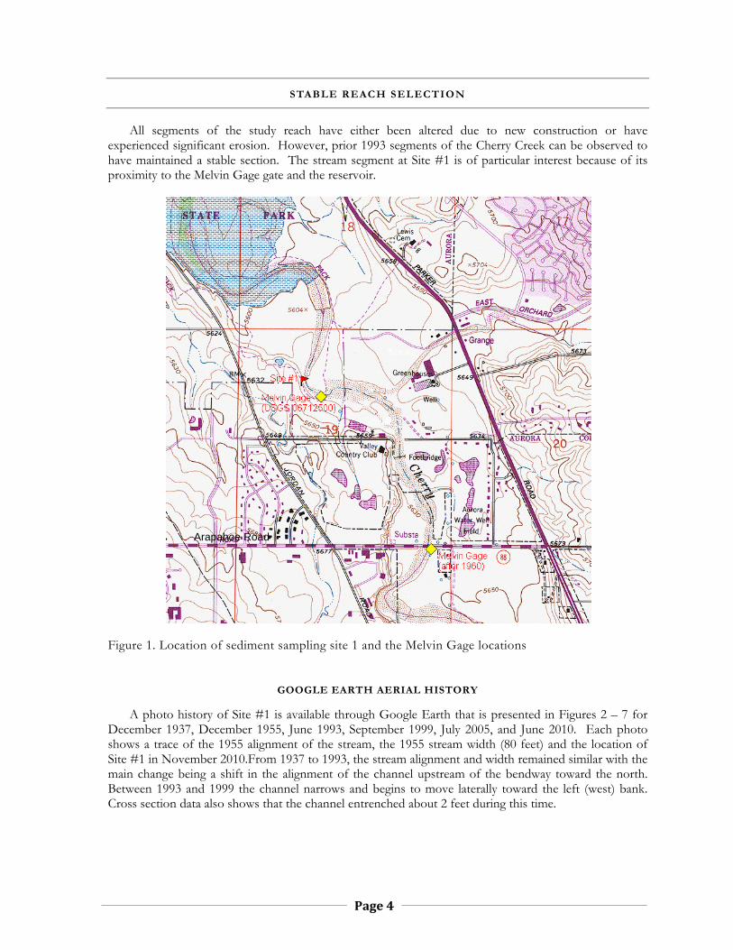
Page 4
STABLE REACH SELECTION
All segments of the study reach have either been altered due to new construction or have experienced significant erosion. However, prior 1993 segments of the Cherry Creek can be observed to have maintained a stable section. The stream segment at Site #1 is of particular interest because of its proximity to the Melvin Gage gate and the reservoir.
Figure 1. Location of sediment sampling site 1 and the Melvin Gage locations
GOOGLE EARTH AERIAL HISTORY
A photo history of Site #1 is available through Google Earth that is presented in Figures 2 – 7 for December 1937, December 1955, June 1993, September 1999, July 2005, and June 2010. Each photo shows a trace of the 1955 alignment of the stream, the 1955 stream width (80 feet) and the location of Site #1 in November 2010.From 1937 to 1993, the stream alignment and width remained similar with the main change being a shift in the alignment of the channel upstream of the bendway toward the north. Between 1993 and 1999 the channel narrows and begins to move laterally toward the left (west) bank. Cross section data also shows that the channel entrenched about 2 feet during this time.
Arapahoe Road

Figure 2. January 1937, Aerial Photograph of Site #1

Page 6
Figure 3. January 1955, Aerial Photograph of Site #1

Page 7
Figure 4. June 1993, Aerial Photograph of Site #1

Page 8
Figure 5. September 1999, Aerial Photograph of Site #1

Page 9
Figure 6. July 2005, Aerial Photograph of Site #1

Page 10
Figure 7. June 2010, Aerial Photograph of Site #1

MELVIN GAGE HISTORY
During the 30 year history of the Melvin gage, the rating curve was shifted 16 times (see Figure 8). These rating shifts accommodated movement in the stream bed that altered the discharge rating for the stream. Indirectly, these shifts also document the pattern of aggradation and degradation the occurred in that same time frame.
Figure 8. Melvin Gage Discharge Rating Curve Shifts
When the shift is plotted over time (Figure 9) it provides a picture of the transient behavior of sediment waves that move through the channel and their frequency. A cycle of about 14 years (crest to crest of trough to trough) can be seen in the shift history. A brief period of scour is followed by a longer period of aggradation. After the gage was relocated in 1960, there was a period of aggradation that abruptly ended with scour during the 1965 flood.
In the Google Earth aerials the 1937 channel appears to be full of sediment; while in 1955 district cut banks can be seen. This agrees with the gage shift record which shows scour approaching 2 feet in 1955.

Page 12
Figure 9. Melvin Gage History
Rat
ing
Shi
ft, fe
et

Page 13
HEC-RAS 4 INPUT
CHANNEL SECTION
Aerial Lidar (Arapahoe County, 2008) was used to cut a cross section near Site #1. The 1940 to 1993 sections was estimated using the measured channel width observed from the 1955 Google Earth and field observation of channel scour and the shift history of the Melvin Gage. Figure 10 shows the original lidar section, the simplified HEC-RAS section and the estimated historic 1937 to 1993 cross section.
Figure 10. Site #1 Cross Section
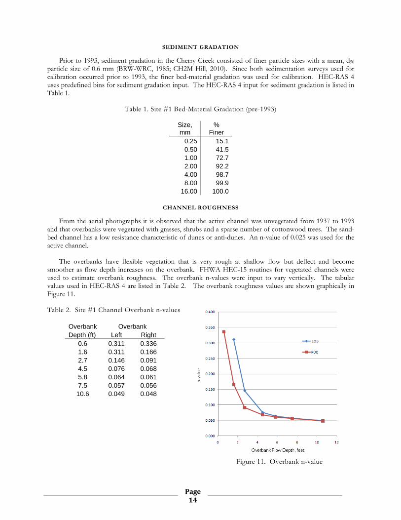
Page 14
SEDIMENT GRADATION
Prior to 1993, sediment gradation in the Cherry Creek consisted of finer particle sizes with a mean, d50 particle size of 0.6 mm (BRW-WRC, 1985; CH2M Hill, 2010). Since both sedimentation surveys used for calibration occurred prior to 1993, the finer bed-material gradation was used for calibration. HEC-RAS 4 uses predefined bins for sediment gradation input. The HEC-RAS 4 input for sediment gradation is listed in Table 1.
Table 1. Site #1 Bed-Material Gradation (pre-1993)
Size, mm
% Finer
0.25 15.10.50 41.51.00 72.72.00 92.24.00 98.78.00 99.9
16.00 100.0
CHANNEL ROUGHNESS
From the aerial photographs it is observed that the active channel was unvegetated from 1937 to 1993 and that overbanks were vegetated with grasses, shrubs and a sparse number of cottonwood trees. The sand-bed channel has a low resistance characteristic of dunes or anti-dunes. An n-value of 0.025 was used for the active channel.
The overbanks have flexible vegetation that is very rough at shallow flow but deflect and become smoother as flow depth increases on the overbank. FHWA HEC-15 routines for vegetated channels were used to estimate overbank roughness. The overbank n-values were input to vary vertically. The tabular values used in HEC-RAS 4 are listed in Table 2. The overbank roughness values are shown graphically in Figure 11.
Table 2. Site #1 Channel Overbank n-values
Overbank Overbank Depth (ft) Left Right
0.6 0.311 0.336 1.6 0.311 0.166 2.7 0.146 0.091 4.5 0.076 0.068 5.8 0.064 0.061 7.5 0.057 0.056 10.6 0.049 0.048
Figure 11. Overbank n-value

Page 15
HEC-RAS 4 RESULTS
SEDIMENT TRANSPORT CAPACITY RATING CURVES
The HEC-RAS 4 hydraulic design tools were used to compute sediment rating curves (sediment transport capacity versus discharge) for six transport relationships available in HEC-RAS 4. For the input channel section, roughness and a range of discharges (from 100 cfs to 50,000 cfs) sediment transport capacity was determined. Sediment inflow was set to equal the transport capacity of the section with a bed slope of 0.0045 ft/ft. Uniform flow hydraulic conditions were computed and each transport equation solved for the same hydraulic conditions.
Figure 12. HEC-RAS derived sediment transport capacity rating curves

Page 16
The resulting rating curves show a wide range of possible sediment transport. At the low end are the Meyer-Peter Muller (MPM) and Toffaleti equations; MPM is a suitable sand bed transport equation but does not account for the suspended portion of the sediment load. Toffaleti is considered a “large” river transport equation and underestimates transport for smaller streams. On this basis the MPM and Toffaleti equations were eliminated from further consideration.
Four relationships are clustered together and each is a suitable transport equation for conditions on the Cherry Creek. The Yang and Ackers-White equations have very similar performance, but the Yang equation is considered to be quite sensitive to channel velocity. Considering that velocities in the Cherry Creek can change quickly, the Yang equation was eliminated from further consideration.
RATING CURVES AS POWER FUNCTIONS
To simplify the use of the rating relationships in calibration, power functions were fitted to the remaining three relationships. Where roughness is rapidly changing (between 2,000 cfs and 5,000 cfs) a power function was not appropriate. This region of the rating curve can be best estimated by using the average of the power functions for the adjacent regions (<2,000 cfs and >5,000 cfs). The general power function equation is given below and Table 3 summarizes the exponents and coefficients for each transport equation.
............................................................................................................................................... Equation 2
Table 3. Power functions of Sediment Transport Capacity
Transport Equation a b Laursen (Copeland) (<2000 cfs) 11.04 1.3897 Laursen (Copeland) (>5000 cfs) 262.19 1.0111
Engelund-Hansen (<2000 cfs) 1.2357 1.6401 Engelund-Hansen (>5000 cfs) 86.235 1.1149
Ackers-White (<2000 cfs) 1.6184 1.5269 Ackers-White (>5000 cfs) 106.76 1.0065
These transport relationships are specifically for the channel geometry and bed-material conditions at Site #1 for the period from 1937 to 1993.
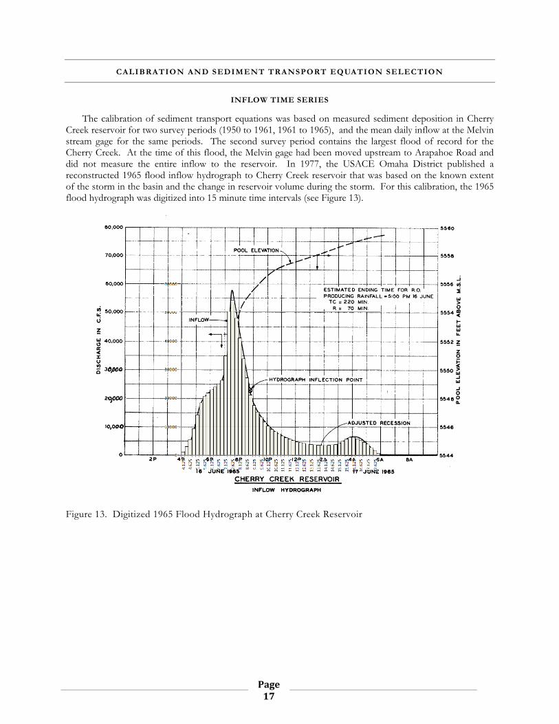
Page 17
CALIBRATION AND SEDIMENT TRANSPORT EQUATION SELECTION
INFLOW TIME SERIES
The calibration of sediment transport equations was based on measured sediment deposition in Cherry Creek reservoir for two survey periods (1950 to 1961, 1961 to 1965), and the mean daily inflow at the Melvin stream gage for the same periods. The second survey period contains the largest flood of record for the Cherry Creek. At the time of this flood, the Melvin gage had been moved upstream to Arapahoe Road and did not measure the entire inflow to the reservoir. In 1977, the USACE Omaha District published a reconstructed 1965 flood inflow hydrograph to Cherry Creek reservoir that was based on the known extent of the storm in the basin and the change in reservoir volume during the storm. For this calibration, the 1965 flood hydrograph was digitized into 15 minute time intervals (see Figure 13).
Figure 13. Digitized 1965 Flood Hydrograph at Cherry Creek Reservoir
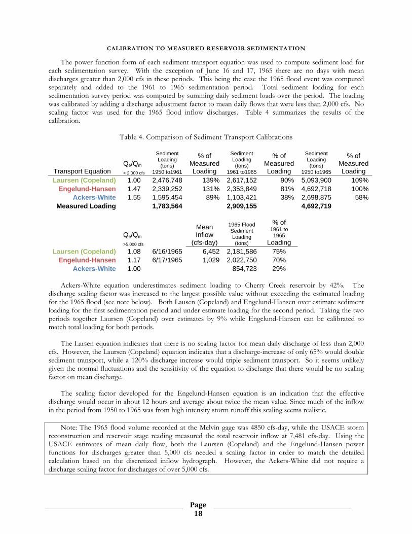
Page 18
CALIBRATION TO MEASURED RESERVOIR SEDIMENTATION
The power function form of each sediment transport equation was used to compute sediment load for each sedimentation survey. With the exception of June 16 and 17, 1965 there are no days with mean discharges greater than 2,000 cfs in these periods. This being the case the 1965 flood event was computed separately and added to the 1961 to 1965 sedimentation period. Total sediment loading for each sedimentation survey period was computed by summing daily sediment loads over the period. The loading was calibrated by adding a discharge adjustment factor to mean daily flows that were less than 2,000 cfs. No scaling factor was used for the 1965 flood inflow discharges. Table 4 summarizes the results of the calibration.
Table 4. Comparison of Sediment Transport Calibrations
Transport Equation Qe/Qm
< 2,000 cfs
Sediment Loading (tons)
1950 to1961
% of Measured Loading
Sediment Loading (tons)
1961 to1965
% of Measured Loading
Sediment Loading (tons)
1950 to1965
% of Measured Loading
Laursen (Copeland) 1.00 2,476,748 139% 2,617,152 90% 5,093,900 109%Engelund-Hansen 1.47 2,339,252 131% 2,353,849 81% 4,692,718 100%
Ackers-White 1.55 1,595,454 89% 1,103,421 38% 2,698,875 58%Measured Loading 1,783,564 2,909,155 4,692,719
Qe/Qm
>5,000 cfs
Mean Inflow
(cfs-day)
1965 Flood Sediment Loading (tons)
% of 1961 to 1965
Loading Laursen (Copeland) 1.08 6/16/1965 6,452 2,181,586 75%
Engelund-Hansen 1.17 6/17/1965 1,029 2,022,750 70% Ackers-White 1.00 854,723 29%
Ackers-White equation underestimates sediment loading to Cherry Creek reservoir by 42%. The
discharge scaling factor was increased to the largest possible value without exceeding the estimated loading for the 1965 flood (see note below). Both Lausen (Copeland) and Engelund-Hansen over estimate sediment loading for the first sedimentation period and under estimate loading for the second period. Taking the two periods together Laursen (Copeland) over estimates by 9% while Engelund-Hansen can be calibrated to match total loading for both periods.
The Larsen equation indicates that there is no scaling factor for mean daily discharge of less than 2,000 cfs. However, the Laursen (Copeland) equation indicates that a discharge-increase of only 65% would double sediment transport, while a 120% discharge increase would triple sediment transport. So it seems unlikely given the normal fluctuations and the sensitivity of the equation to discharge that there would be no scaling factor on mean discharge.
The scaling factor developed for the Engelund-Hansen equation is an indication that the effective discharge would occur in about 12 hours and average about twice the mean value. Since much of the inflow in the period from 1950 to 1965 was from high intensity storm runoff this scaling seems realistic.
Note: The 1965 flood volume recorded at the Melvin gage was 4850 cfs-day, while the USACE storm reconstruction and reservoir stage reading measured the total reservoir inflow at 7,481 cfs-day. Using the USACE estimates of mean daily flow, both the Laursen (Copeland) and the Engelund-Hansen power functions for discharges greater than 5,000 cfs needed a scaling factor in order to match the detailed calculation based on the discretized inflow hydrograph. However, the Ackers-White did not require a discharge scaling factor for discharges of over 5,000 cfs.
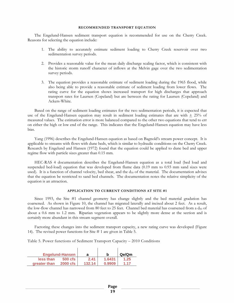
Page 19
RECOMMENDED TRANSPORT EQUATION
The Engelund-Hansen sediment transport equation is recommended for use on the Cherry Creek. Reasons for selecting the equation include:
1. The ability to accurately estimate sediment loading to Cherry Creek reservoir over two sedimentation survey periods.
2. Provides a reasonable value for the mean daily discharge scaling factor, which is consistent with the historic storm runoff character of inflows at the Melvin gage over the two sedimentation survey periods.
3. The equation provides a reasonable estimate of sediment loading during the 1965 flood, while also being able to provide a reasonable estimate of sediment loading from lower flows. The rating curve for the equation shows increased transport for high discharges that approach transport rates for Laursen (Copeland) but are between the rating for Laursen (Copeland) and Ackers-White.
Based on the range of sediment loading estimates for the two sedimentation periods, it is expected that use of the Engelund-Hansen equation may result in sediment loading estimates that are with + 25% of measured values. The estimation error is more balanced compared to the other two equations that tend to err on either the high or low end of the range. This indicates that the Engelund-Hansen equation may have less bias.
Yang (1996) describes the Engelund-Hansen equation as based on Bagnold’s stream power concept. It is applicable to streams with flows with dune beds, which is similar to hydraulic conditions on the Cherry Creek. Research by Engelund and Hansen (1972) found that the equation could be applied to dune bed and upper regime flow with particle sizes greater than 0.15 mm.
HEC-RAS 4 documentation describes the Engelund-Hansen equation as a total load (bed load and suspended bed-load) equation that was developed from flume data (0.19 mm to 0.93 mm sand sizes were used). It is a function of channel velocity, bed shear, and the d50 of the material. The documentation advises that the equation be restricted to sand bed channels. The documentation notes the relative simplicity of the equation is an attraction.
APPLICATION TO CURRENT CONDITIONS AT SITE #1
Since 1993, the Site #1 channel geometry has change slightly and the bed material gradation has coarsened. As shown in Figure 10, the channel has migrated laterally and incised about 2 feet. As a result, the low-flow channel has narrowed from 80 feet to 25 feet. Channel bed material has coarsened from a d50 of about a 0.6 mm to 1.2 mm. Riparian vegetation appears to be slightly more dense at the section and is certainly more abundant in this stream segment overall.
Factoring these changes into the sediment transport capacity, a new rating curve was developed (Figure 14). The revised power functions for Site # 1 are given in Table 5.
Table 5. Power functions of Sediment Transport Capacity – 2010 Conditions
Engelund-Hansen a b
Qe/Qm
less than 500 cfs 2.41 1.6431 1.25 greater than 2000 cfs 132.14 0.9909 1.17

Page 20
Figure 14. Revised Site #1 Sediment Rating Curve
Mean daily flow data from the C-10 gage (January 1992 to December 2009) was used compare the sediment loading for current conditions and conditions before 1993. During this time period, mean daily inflow to the reservoir did not exceed 352 cfs and so sediment transport capacity is described by the lower power function of the sediment rating curve. The discharge scaling factor was set at 1.25 for both rating curves to account for increased based flow.
Total water inflow in this 18 year time period was 135,908 ac-ft. Using the pre-1993 rating curve, the estimated sediment loading to the reservoir is 1,087,117 tons (525 ac-ft). By comparison, the current 2010 rating results in an estimated sediment loading to the reservoir of 2,146,485 tons (1,037 ac-ft) or approximately twice the sediment load. The current rating is not therefore a stable one and shows that the stream section is now in transition to a new equilibrium. This site should no longer be used as a boundary condition for estimating sediment loading conditions to the reservoir.
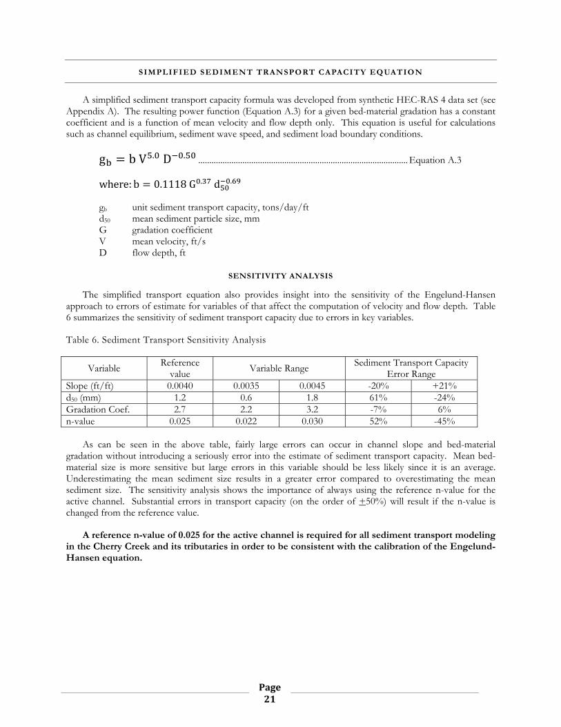
Page 21
SIMPLIFIED SEDIMENT TRANSPORT CAPACITY EQUATION
A simplified sediment transport capacity formula was developed from synthetic HEC-RAS 4 data set (see Appendix A). The resulting power function (Equation A.3) for a given bed-material gradation has a constant coefficient and is a function of mean velocity and flow depth only. This equation is useful for calculations such as channel equilibrium, sediment wave speed, and sediment load boundary conditions.
g b V . D . ............................................................................................... Equation A.3
where: b 0.1118 G . d .
gb unit sediment transport capacity, tons/day/ft d50 mean sediment particle size, mm G gradation coefficient V mean velocity, ft/s D flow depth, ft
SENSITIVITY ANALYSIS
The simplified transport equation also provides insight into the sensitivity of the Engelund-Hansen approach to errors of estimate for variables of that affect the computation of velocity and flow depth. Table 6 summarizes the sensitivity of sediment transport capacity due to errors in key variables.
Table 6. Sediment Transport Sensitivity Analysis
Variable Reference value Variable Range Sediment Transport Capacity
Error Range Slope (ft/ft) 0.0040 0.0035 0.0045 -20% +21% d50 (mm) 1.2 0.6 1.8 61% -24% Gradation Coef. 2.7 2.2 3.2 -7% 6% n-value 0.025 0.022 0.030 52% -45%
As can be seen in the above table, fairly large errors can occur in channel slope and bed-material
gradation without introducing a seriously error into the estimate of sediment transport capacity. Mean bed-material size is more sensitive but large errors in this variable should be less likely since it is an average. Underestimating the mean sediment size results in a greater error compared to overestimating the mean sediment size. The sensitivity analysis shows the importance of always using the reference n-value for the active channel. Substantial errors in transport capacity (on the order of +50%) will result if the n-value is changed from the reference value.
A reference n-value of 0.025 for the active channel is required for all sediment transport modeling in the Cherry Creek and its tributaries in order to be consistent with the calibration of the Engelund-Hansen equation.

Page 22
SUMMARY OF RESULTS
From study field reconnaissance, and review of Google Earth images (from 1937 to 2010) it was determined that the stream segment of the Cherry Creek near Site #1 had a relatively stable cross section between 1937 to 1993. Using a cross section at Site #1 derived from 2008 aerial lidar data and adjusting for lateral erosion and scour that had occurred since 1993, the historic stream cross section was reconstructed. Historic sediment gradation was estimated from 1985 and 2010 samples of the Cherry Creek stream bed. The channel roughness was estimated based on the observed unvegetated width of channel and estimated vegetation coverage. The channel hydraulic conditions were computed over a range of discharges using a vertical change in roughness to simulated the affected of vegetation on the overbank.
Using HEC-RAS 4’s hydraulic design tools, six sediment transport capacity rating curves were developed for the historic conditions. Of these three equations were selected for further evaluation: Laursen (Copeland), Engelund-Hansen, and Ackers-White. For more convenient computation, the rating curves were converted to power functions.
The sediment transport equations were compared to measured sediment deposition in Cherry Creek reservoir for two periods (1950 to 1961, 1961 to 1965). Sediment load was estimated for the sedimentation periods using the inflow time series at the Melvin stream gage and the 1965 June flood inflow hydrograph. Based on this analysis the Engelund-Hansen equation was found to most closely estimate the sedimentation history from 1950 to 1965.
A simplified version of the Engelund-Hansen sediment transport equation was developed as a power function. A sensitivity analysis was conducted using the power function version of the Engelund-Hansen sediment transport equation that shows the potential affect on sediment transport capacity estimations caused by errors in key hydraulic variables. Other potential uses of the simplified equation include: equilibrium analysis, estimation of sediment wave speed, and estimation of boundary conditions.

Page 23
REFERENCES
BRW Inc. -WRC Engineering, Inc, 1985, “Feasibility Study for the Cherry Creek Basin Drainageway” prepared for Cherry Creek Basin Technical Advisory Committee and Parker-Jordan Metropolitan District
CH2M HILL, 2010, “Cherry Creek at 12-Mile Park (Draft)/ Site Assessment Report”, prepared for Cherry Creek Basin Water Quality Authority
Engelund, F., 1973, “Steady transport on moderately graded sediment,” Institute of Hydrodynamics and Hydraulic Engineering, Technical University of Denmark, Progress Report 21
Engelund, F. and E. Hansen, 1967, “A Monograph on Sediment Transport in Alluvial Streams”, Teknisk Forlag, Copenhagen
HEC-RAS Version 4.0, March 2008, “River Analysis System Application Guide” U.S. Army Corps of Engineers, Hydrologic Engineering Center, Davis, CA
Microsoft Office Excel 2007, Microsoft Corporation
USACE-Omaha District, 1977, “Review Report for Water and Related Land Resources Management Study / Metropolitan Denver and South Platte River and Tributaries / Colorado, Wyoming and Nebraska”
USACE-Omaha District, 2001, “Tri-Lakes Sediment Studies” M.R.B Sediment Memorandum 23
Yang, Chih Ted, 1996, Sediment Transport, Theory and Practice, McGraw-Hill

Page 24
APPENDIX A. SIMPLIFIED ENGELUND AND HANSEN SEDIMENT TRANSPORT CAPACITY EQUATION
ENGELUND AND HANSEN’S APPROACH
Engelund and Hansen (1967) proposed a method for determining total sediment load in streams with dune-covered beds. The relationships are as follows:
f 0.1 θ . ........................................................................................................... Equation A.1
:
S ............................................................................................... Equation A.1.1
f UU
.............................................................................................................. Equation A.1.2
UU
0.6 2.5 ln ................................................................ Equation A.1.2.1
where: k 2.5 d
y y .......................................................................................... Equation A.1.3.1
θ ................................................................................................... Equation A.1.3.2
θ 0.06 0.4 θ ..................................................................... Equation A.1.3.2
With the value of y’o the mean velocity, U, can be calculated. The sediment load can then be expressed as:
g 0.05 U S
/ .................................................................. Equation A.2
where:
d50 mean sediment particle size, mm df equivalent particle size based on fall velocity, mm gb unit sediment transport capacity, tons/day/ft g acceleration of gravity, ft/s2 k equivalent roughness size, ft S’s submerged specific gravity of sediment, dimensionless S Slope, ft/ft U* shear velocity, ft/s U, V mean velocity, ft/s w fall velocity, ft/s y’o effective flow depth, ft γ’s submerged unit weight of sediment, lb/ft3
τo bed shear stress, lb/ft2

Page 25
Engelund (1973) also proposed a method for calculation of sediment transport when the bed material is graded. It assumed that particles finer than a certain size will all enter into suspension while larger grains will move as bed load. The criterion for critical size is based on the empirical value of 2.5 2.
E-H SEDIMENT TRANSPORT CAPACITY FROM HEC-RAS 4
While the Engelund and Hansen is not a particularly complex sediment transport formula, there are several aspects of the approach that require detailed knowledge to implement in HEC-RAS 4. So as not to presume the approach taken by HEC, a set of sediment transport capacity data was generated directly from HEC-RAS 4.
Input consisted of a wide rectangular channel (50 feet) with a uniform n-value of 0.025 for the geometry. Increments of channel slope varied as 0.0020, 0.0040 and 0.0060 ft/ft. The gradation of the bed material was varied from d50 of 0.6 mm to 1.9 mm with gradation coefficients of 2.2 and 3.2 for the 1.9 mm size. Unit discharge was varied from 1.0 cfs/ft to 200 cfs/ft.
Table A.1 summarizes the input increments for the Engelund and Hansen sediment transport calculations using HEC-RAS 4. The generated data set is given at the end of this Appendix.
Table A.1. HEC-RAS 4 Input Cases
Case Slope, S (ft/ft)
d50 (mm) G Unit discharge, q, increments (cfs/ft)
1 0.0020
0.6
2.2
1, 2, 5, 10, 20, 50, 100, 200
2 0.0040
3 0.0060
4 0.0020
1.2 5 0.0040
6 0.0060
7 0.0020
1.6 8 0.0040
9 0.0060
10 0.0020
1.9 3.2 11 0.0040
12 0.0060

Page 26
E-H SEDIMENT TRANSPORT CAPACITY REGRESSION EQUATION
A sediment transport capacity regression equation was computed by transforming the data set (total bed load, mean velocity, depth, and mean sediment size) to natural log values and then linearly regressing the transformed data set using Excel’s LINEST regression function. Since the data set is without error and derived from a fairly simple function it was expected that regression error should be minimal. The r2 value for the equations was in fact 1.0. The resulting power function formula is
g b V . D . ............................................................................................... Equation A.3
where: b 0.1118 G . d .
The coefficient, b, is constant for a known sediment gradation. For example, current bed-material in the Cherry Creek has the following properties: d50 = 1.2 and G = 2.2, which give a coefficient of b = 0.132. Up-valley the bed-material coarsens to d50 = 1.9 and G = 3.2, which give a coefficient of b = 0.110 (about a 20% reduction).
Of interest in equation 3 are the two exponents. The velocity exponent of 5.0 can be predicted from equation 2, since τ U . This indicates that the formula has a very high sensitivity to velocity. The flow depth exponent shows a common behavior of sediment transport, which is a reduction in transport capacity with increasing flow depth.
RANGE OF APPLICABILITY
As with any regression equation, the use of the Engelund-Hansen regression equation should not exceed the range of data from which it was developed. This is particularly true for the properties of the sediment gradation (G and d50). Likewise, when using this regression equation to estimate sediment transport in the active channel of the Cherry Creek, the active channel roughness should always be 0.025 to be consistent with the active-channel roughness that was used to develop this data set.
The ranges are applicable to the hydraulic properties of the active channel of the Cherry Creek and do not necessarily apply to portions of the channel that are outside that boundary where sediment transport is not being calculated.
Variable Range Sediment size, d50 (mm) 0.6 to 1.9 Gradation Coefficient, G 2.2 to 3.2 Velocity, V (ft/s) 1.8 to 20.8 Depth, D (ft) 0.4 to 13.3 Froude No., Fr 0.4 to 1.2 Unit discharge, q (cfs/ft) 1 to 200 Slope, S (ft/ft) 0.0020 to 0.0060

Page 27
HEC-RAS 4 DATA SET
Case G d50
(mm) S
(ft/ft) q
(cfs/ft) gb
(tons/day/ft)
V (ft/s)
D (ft)
1 2.2 0.6 0.002
1 5.3 1.8 0.56 2 17.3 2.37 0.84 5 82.1 3.42 1.46
10 267.0 4.51 2.21 20 868.4 5.96 3.35 50 4118 8.59 5.81
100 13350 11.33 8.8 200 43320 14.95 13.34
2 2.2 1.2 0.002
1 3.3 1.8 0.56 2 10.8 2.37 0.84 5 51.3 3.42 1.46
10 166.8 4.51 2.21 20 542.6 5.96 3.35 50 2574 8.59 5.81
100 8344 11.33 8.8 200 27060 14.95 13.34
3 2.2 1.6 0.002
1 2.7 1.8 0.56 2 8.7 2.37 0.84 5 41.4 3.42 1.46
10 134.6 4.51 2.21 20 438 5.96 3.35 50 2076 8.59 5.81
100 6734 11.33 8.8 200 21840 14.95 13.34
4 2.2 0.6 0.004
1 16.9 2.21 0.45 2 54.7 2.92 0.69 5 258.8 4.21 1.19
10 839 5.56 1.8 20 2724 7.33 2.73 50 12928 10.58 4.72
100 41940 13.96 7.15 200 136240 18.41 10.83
5 2.2 1.2 0.004
1 10.6 2.21 0.45 2 34.2 2.92 0.69 5 161.7 4.21 1.19
10 524.2 5.56 1.8 20 1702.2 7.33 2.73 50 8080 10.58 4.72
100 26200 13.96 7.15 200 85140 18.41 10.83

Page 28
(continued)
Case G d50
(mm) S
(ft/ft) q
(cfs/ft) gb
(tons/day/ft)
V (ft/s)
D (ft)
6 2.2 1.6 0.004
1 8.5 2.21 0.45 2 27.6 2.92 0.69 5 130.5 4.21 1.19
10 423.2 5.56 1.8 20 1373.8 7.33 2.73 50 6520 10.58 4.72
100 21160 13.96 7.15 200 68720 18.41 10.83
7 2.2 0.6 0.006
1 33.2 2.5 0.4 2 103.6 3.3 0.61 5 503 4.76 1.05
10 1638.8 6.28 1.59 20 5318 8.28 2.41 50 25240 11.95 4.18
100 81880 15.71 6.35 200 266000 20.78 9.6
8 2.2 1.2 0.006
1 20.7 2.5 0.4 2 64.8 3.3 0.61 5 314.4 4.76 1.05
10 1024.2 6.28 1.59 20 3324 8.28 2.41 50 15772 11.95 4.18
100 51180 15.71 6.35 200 166240 20.78 9.6
9 2.2 1.6 0.006
1 16.7 2.5 0.4 2 52.3 3.3 0.61 5 253.8 4.76 1.05
10 826.6 6.28 1.59 20 2682 8.28 2.41 50 12730 11.95 4.18
100 41300 15.71 6.35 200 134180 20.78 9.6

Page 29
(continued)
Case G d50 (mm)
S (ft/ft)
q (cfs/ft)
gb (tons/day/ft)
V (ft/s)
D (ft)
10 3.2 1.9 0.002
1 2.8 1.80 0.56 2 9.0 2.37 0.84 5 42.7 3.42 1.46
10 138.9 4.51 2.21 20 451.8 5.96 3.35 50 2142 8.59 5.81
100 6946 11.33 8.8 200 22540 14.95 13.34
11 3.2 1.9 0.004
1 8.8 2.21 0.45 2 28.5 2.92 0.69 5 134.6 4.21 1.19
10 436.6 5.56 1.8 20 1417.2 7.33 2.73 50 6726 10.58 4.72
100 21820 13.96 7.15 200 70900 18.41 10.83
12 3.2 1.9 0.006
1 17.3 2.5 0.4 2 53.9 3.3 0.61 5 261.8 4.76 1.05
10 852.8 6.28 1.59 20 2768 8.28 2.41 50 13132 11.95 4.18
100 42600 15.71 6.35 200 138420 20.78 9.6

C h e r r y C r e e k S e d i m e n t a t i o n S t u d y R e s e r v o i r t o P i n e L a n e
S e d i m e n t B u d g e t
March 2011 Prepared for: Southeast Metropolitan Stormwater Authority 76 Inverness Drive Englewood, Colorado Submitted to: Ms. Molly Trujillo, P.E. Prepared by:
GK COTTON CONSULTING, INC 10290 S. Progress Way, #205 PO Box 1060 Parker, CO 80134-1060

C H E R RY C R E E K S E D I M E N TAT I O N S T U DY
SEDIMENT BUDGET
Table of Contents
Introduction............................................................................................................................. 3
Description of Water Operations ............................................................................................. 3
CCBWQA Model Structure ................................................................................................................ 4
Flow Pattern .................................................................................................................................... 4
Sub‐Reach Characteristics ........................................................................................................ 5
Sediment Transport Ratings .................................................................................................... 7
HEC‐RAS Results ............................................................................................................................... 7
Time Step Scaling ............................................................................................................................. 8
Sediment Budget ..................................................................................................................... 9
Supply Reach .................................................................................................................................... 9
Sediment Budget by Sub‐Reach ...................................................................................................... 12
Summary and Findings .......................................................................................................... 14
References ............................................................................................................................. 14
Appendix A. Sub‐Reach Cross Sections ................................................................................... 15
Appendix B. Sub‐Reach Hydraulic Design Data / Sediment Transport Rating ......................... 21
Appendix C. Sub‐Reach Flow Data from CCBWQA Model ....................................................... 33
Appendix C. Sub‐Reach Sediment Transport Capacity ............................................................ 41

Page 3
INTRODUCTION
This paper discusses the sediment budget of the Cherry Creek from near the confluence of Baldwin Gulch (Pine Lane bridge over the Cherry Creek) to the Piney Creek confluence (southern boundary of Cherry Creek State Park). The discussion focuses on the period from 1992 to 2002 for which there is a calibrated simulation of water operations in the Cherry Creek (2008, Brown & Caldwell) that was developed by the Cherry Creek Basin Water Quality Authority (CCBWQA). The simulation provides mean monthly time series for 11 stream sub-reaches, which provides a more detailed stream hydrology than can be provide by existing gages that are located at Parker and within Cherry Creek reservoir.
Sediment inflow is estimated at the upper sub-reach. This rating is expected to be stable given the recent observations of channel behavior and stream stabilization measures that have been constructed in this stream segment. Sediment transport capacity for sub-reaches is based on channel gradients and characteristic channel sections. Channel sections were derived from 2008 LiDaR topography. Some adjustments were made to sections, when needed to make the section more representative. For example, some channel sections have temporarily scoured but now have been or will shortly be repaired. Sediment transport capacity ratings for the sub-reaches were developed using HEC-RAS 4 design tools with the Engelund-Hansen formula.
Sediment budget was calculated on a monthly basis for each sub-reach and the potential volume of reach aggradation / scour computed. A discharge-scaling term was estimated from daily and monthly flow records at the Parker stream gage and then applied to the monthly time series simulation for estimation of mean monthly sediment transport capacity.
It was found that the study reach looses stream flow at the rate of about 6.3% per mile relative to inflow at the confluence of Baldwin Gulch (near Parker, CO). Over the simulation period, 32% of inflow is diverted by water suppliers as well as inflows from stormwater runoff and return flows. These diversions occur from the alluvial aquifer of the Cherry Creek valley via well fields that are operated by water providers. As a result, 67% of the sediment supply that enters the study reach is deposited within the study reach. Most of the study sub-reaches are depositional with the exception of the sub-reach below the confluence of Happy Canyon Wash, which is scour prone.
DESCRIPTION OF WATER OPERATIONS
The current pattern of stream flow in the Cherry Creek above the reservoir is complex and continuously changing as water supply providers expand to meet the demand of new development in the watershed. Both the surface flows and flows in the alluvium of the channel are affected by this water development. The alluvial aquifer plays an important role in water operations as the means of diverting decreed alluvial water and in recovering re-useable return flows. Alluvial groundwater is captured by an extensive array of shallow wells along the valley floor. So, unlike many stream in Colorado where surface diversion structures are common, diversions from the Cherry Creek are predominantly made by well fields.
As a result, stream flow in the Cherry Creek cannot be well understood by the measurement of surface stream flow alone. As water demand increases in the basin, it is projected (South Metro Water Supply Authority Regional Master Plan) that use of non-tributary groundwater will decrease and will be replaced by renewable imported water and recaptured flows. Water from the basin itself will be fully used such that most flow that will be carried in the stream will originate from storm runoff and return flows. Since return flows are derived from water imported to the basin (either from non-tributary groundwater or imported renewable water rights), these flows can be reused completely by the water provider and are not subject to calls from downstream water users. The ability to recover return flow is important to meeting future water demand.

Page 4
Since the early 1990s, stream flow in the Cherry Creek above the reservoir has increased and groundwater elevations in the alluvial aquifer are higher. The result has been increased riparian vegetation and a general improved quality of stream ecology compared to the dry stream bed that existed for the prior century or longer. Modeling by CCBWQA shows that alluvial aquifer levels will remain at a healthy elevation in the Cherry Creek, although the pattern of base stream flow will not be particularly natural.
It is unlikely that water development will cause the stream to dry up for several reasons. First, although the Cherry Creek alluvium plays an important role in recovering return flow, it does not have a substantial amount of water storage capacity (perhaps around 5,000 ac-ft between Parker and the southern boundary of the reservoir). Second, CCBWQA modeling shows relatively constant down valley flow in the alluvium, indicating that it is being used primarily as a means of collecting flows and not as a water supply. In drought years, depletion of alluvial groundwater would be of marginal benefit and would probably make it more difficult to recover return flows.
Sustained groundwater elevations in the alluvium will be important to the riparian plant community. So while surface flows may vary significantly, groundwater elevations should ensure that larger riparian plants weather drought conditions in the watershed.
CCBWQA MODEL STRUCTURE
The CCBWQA model derives its spatial topology from the UDFCD UDSWM model that was developed for stormwater master planning and flood hazard delineation (Figure 1 below shows the portion of the UDSWM model schematic for the study reach). The CCBWQA model simulates frequent runoff, flow in alluvium, and contaminant (phosphorus) loading that were not part of the original UDSWM model. The CCBWQA model does not simulate flood hydrology. The master plan model ended above the Piney Creek confluence, so the CCBWQA adds in tributaries that confluence within the state park or drain directly to the reservoir.
Figure 1. CCBWQA model structure for the study reaches
FLOW PATTERN
Gage data between the Parker and CC-10 gage show that the study reach looses flow. The CCBWQA model shows (Figure 2) this loss process in more detail. As discussed previously, the loosing reach behavior is the result of pumping from alluvial wells and is part of water supply operations by water providers. Figure 2, shows an underlying loss rate of about 6.3% per mile (red line) that results in 32% depletion of stream flow between Parker and Valley Country Club (relative to upstream inflow). This general pattern is interrupted by larger tributary inflows including Happy Canyon Wash and three unnamed tributaries below Chenango.

Page 5
Figure 2. Loosing reach behavior for the Cherry Creek below Parker, CO
SUB-REACH CHARACTERISTICS
Characteristics of each sub-reach included stream slope, reach length, channel cross section, un-vegetated active channel width, active channel width, and fall at structures (see Table 1). With the exception of reach length, which was obtained from the master plan, all these data were measured for this study either in the field (un-vegetated active channel width), 2008 LiDaR topography (channel cross section, stream slope, active channel width, invert elevation). There is a 12 foot difference between elevation change due to stream slope between the master plan and this study. The smaller changes are within the LiDaR accuracy (+ 1.0 foot), while larger changes are due to the construction of drop structures and other grade controls since 2002.
Stream slopes measured for this study were found to be in a narrower range than was reported in the Master Plan, averaging 0.0395 +0.00043 ft/ft compared to 0.00444 +0.0007. Outside of the un-vegetated active channel, roughness was varied vertically to account for the change in roughness of flexible riparian vegetation as flow depth increases (Table 2). Bedload gradation was varied between the un-vegetated active channel width (coarser gradation) and the remainder of the cross section (Table 3). Channel cross sections are plotted and tabulated in Appendix A.

Page 6
Table 1. Sub-Reach Characteristics
Sub-Reach
Invert Elev
Study Slope (ft/ft)
MP Slope (ft/ft)
MP Fall (ft)
Reach Length
(ft)
Un-Veg ActWid
(ft)
Slope Fall (ft)
MP-Stdy Fall Diff.
(ft) 880 5750.0 0.00379 0.00450 9.5 2180 15 8.0 1.5
878 5746.0 0.00457 0.00500 8.7 1715 35 8.0 0.7
873 5720.0 0.00472 0.00440 28.0 5270 35 30.0 -2.0
869 5704.0 0.00383 0.00440 4.6 1032 35 4.0 0.6
867 5700.0 0.00438 0.00470 3.0 2615 35 2.8 0.2
868 5694.0 0.00400 0.00380 9.3 696 35 14.0 -4.7
819 5676.0 0.00358 0.00280 9.4 2353 39 12.0 0.0
816 5654.0 0.00350 0.00500 35.0 5657 25 24.5 10.0
821 5638.0 0.00345 0.00450 18.9 2903 25 14.5 4.4
813 5628.0 0.00332 0.00520 7.2 1378 25 4.6 2.6
812 5624.0 0.00388 0.00520 3.2 627 25 2.4 0.8 Table 2. Vertical variation in roughness with flow depth
Depth n-value (ft) Left Main Right
0.0 0.311 0.025 0.311
1.0 0.311 0.025 0.311
2.0 0.146 0.025 0.146
4.0 0.076 0.025 0.076
5.0 0.064 0.025 0.064
7.0 0.057 0.025 0.057
10.0 0.049 0.025 0.049
Table 3. Bed material gradation properties
Grain size % Finer
(mm) Left Main Right 0.25 15.1 2.5 15.1
0.5 41.5 14.0 41.5
1.0 72.7 42.1 72.7
2.0 92.2 75.2 92.2
4.0 98.7 94.1 98.7
8.0 99.9 99.3 99.9
16.0 100.0 100.0 100.0

Page 7
SEDIMENT TRANSPORT RATINGS
HEC-RAS RESULTS
Rating curves were developed for each sub-reach by using the HEC-RAS 4 hydraulic design tool for sediment transport capacity. A set of increasing discharges from 10 cfs to 10,000 cfs was input as the flow range. A simple three cross section reach was created by repeating the sub-reach cross section at 100 foot intervals and offsetting section by the sub-reach stream slope. Hydraulic design output for each sub-reach is listed in Appendix B.
Figure 3. Sub-Reach Sediment Transport Rating Curves
The sediment ratings show similar pattern particularly in the lower range of flow (less than 500 cfs) but still differ from each other by as much as a factor of three times. The rating for sub-reach 813 is the lowest of all rating. This sub-reach includes the Arapahoe Road bridge and Valley Country Club, which have had a history of aggradation. The ratings were not simplified by curve fitting and were used in sediment budgeting analysis with the Excel table lookup function. Log interpolation was used for discharges greater than 10 cfs and linear interpolation was used for discharges between 0 and 10 cfs.

Page 8
TIME STEP SCALING
The sediment budget analysis was conducted at monthly time steps; however, the sediment transport function is an instantaneous measurement. To account for the variations in flow within a monthly time step, a scaling analysis was conducted using the Parker gage (USGS 393109104464500 CHERRY CREEK NEAR PARKER, CO).
The sediment rating for the sub-reaches was computed from mean-daily discharges by first multiplying the daily discharges by 1.25 (in accordance with the sediment transport calibration of the Engelund-Hansen equation). Next, the mean-monthly discharges were scaled by a factor, such that the total monthly volume of sediment closely matched the volume computed for sum of the daily sediment volumes for a month. The result was a scaling factor of 1.352. The sediment volume computed using a monthly time step was within 0.4% of the volume computed using a daily time step. For the period from 1995 to 2002, scatter was also low with an R2 value of 0.9878. Figure 4 shows the relationship between daily and monthly time step scaling.
Figure 4. Estimates of sediment volume using daily and scaled monthly time steps

Page 9
SEDIMENT BUDGET
SUPPLY REACH
The upper most sub-reach is 880, which is located at the Pine Lane bridge over the Cherry Creek. As with other areas of the Cherry Creek, the active channel has changed significantly since the early 1990’s becoming significantly more vegetated (Figure 5). As the un-vegetated narrowed and base flows increased, this reach developed minor scour problems in the low-flow channel. With the construction of the new bridge, small checks were constructed in the low-flow channel and the scour has been repaired (Figure 6).
The 2008 topographic data reflects a stable condition that can be used to characterize upstream sediment supply to the study reach. This sub-reach has a stream gradient and active channel width that are close to the averages for the overall reach. The unvegetated portion of the active channel width is narrower compared to the other downstream sub-reaches.
The history of sediment loading for this reach is shown in Figure 7 for the simulation period. The pattern of sediment transport follows that of stream flow and so periods of low sediment transport correspond to periods of low stream flow. Histograms of monthly water and sediment loading (Figures 8 and 9) show this pattern. For the eight year simulation period, total sediment transport from this reach is 1.11 million tons (538 ac-ft).
Figure 5. Sub-reach 880 c. 1994

Page 10
Figure 6. Sub-reach 880 c. 2010
Figure 7. Sediment transport from sub-reach 880

Page 11
Figure 8. Discharge Histogram for sub-reach 880
Figure 9. Sediment Loading Histogram for sub-reach 880

Page 12
SEDIMENT BUDGET BY SUB-REACH
Sediment transport capacity in the study reach steadily decreases in the downstream direction (Figure 10). This creates the potential for aggradation for most sub-reaches. Sub-reach 867, which is located below the Happy Canyon confluence, is the exception to this trend. Sub-reach 812 is a short contracted reach of the Cherry Creek upstream of Caley Avenue that has a locally higher transport capacity and a strong potential to scour. While there has been scour in the stream segment below Happy Canyon, the 812 sub-reach does not show scour. The approach of using uniform flow for the 812 sub-reach is probably not accurate since it does not account for the backwater created by the Caley Avenue constriction of the stream channel.
Figure 10 shows the cumulative transport of sediment for the eight year study period. On an annual basis, there is an average of 2.1 tons (1.6 cubic yards) of sediment depositing per foot of stream length per year within the active channel of the Cherry Creek. Relative to the transport capacity of the Cherry Creek at Parker, only 33% of that capacity remains at the most sub-reach 813.
Figure 10. Sediment Budget by Sub-Reach and Potential Aggradation/Scour

Page 13
As an example of the detailed aggradation/degradation behavior of a sub-reach, reach 867 and 813 are shown in Figure 11. These time series show that while a sub-reach tends to be predominantly aggradational or degradational, there are never-the-less periods where the trend reverses (highlighted in yellow). While a lack of sediment supply to a reach results in channel erosion, erosion still occurs in aggrading reaches as the stream reworks the excess sediment load. Large deposits of sediment in a reach often cause a shift in stream pattern, which can trigger erosion.
Figure 11. Aggradation / Degradation Time Series for selected sub-reaches (867 and 813), yellow highlights show periods of scour in a predominantly aggrading reach or periods of aggradation in a predominantly scouring reach.

Page 14
SUMMARY AND FINDINGS
1. The CCBWQA hydrology simulation provided eight years of flow data for the study reach. In addition, the simulation provides detailed routing for 11 sub-reaches following the routing topology that was developed for floodplain master planning (URS, 2002).
2. The hydrology simulation shows that the study reach looses flow to water diversion at the rate of 6.3% per mile. Tributary inflow are quickly diverted and as a result have a fairly localize affect on the water balance.
5. Channel cross-section, stream gradient, and cross section properties (sediment gradations and roughness) were developed for each of the 11 sub-reaches of the study reach.
3. Mean monthly discharge was scaled by a factor of 1.352 for estimation of mean-monthly sediment load. This allowed the use of CCBWQA mean-monthly flow data.
4. The upper sub-reach of the study area (sub-reach 880) was found to be stable and it is recommended as a reliable reach for the estimation of incoming sediment supply to the study reach.
6. The sediment budget for the study sub-reaches shows that transport capacity steadily decreases in the downstream direction. This is directly attributable to the reduction in flow in the Cherry Creek. Only the sub-reach below Happy Canyon showed a potential for scour.
REFERENCES
CDM, 2007, “South Metro Water Supply Authority Regional Water Master Plan” prepared for South Metro Water Supply Authority
Brown and Caldwell, 2008, “Cherry Creek Basin Watershed Phosphorus Model Documentation” prepared for the Cherry Creek Basin Water Quality Authority

Page 15
APPENDIX A. SUB-REACH CROSS SECTIONS
Table 4. Cross section topwidth (blue values are the approximate width of the active channel)
Depth (ft) 880 878 873 869 867 868 8190.0 15 107 35 13 57 23 312.0 265 274 479 115 256 79 1664.0 583 901 504 356 288 704 1776.0 619 1071 610 388 319 736 1878.0 1227 859 898 198
Depth (ft) 816 821 813 812 Low Avg High 0.0 41 123 123 17 30 67 1352.0 106 371 371 100 113 237 3404.0 407 429 474 113 268 450 6016.0 628 488 485 173 310 539 7298.0 720 937 459 807 1021

Page 16

Page 17

Page 18

Page 19

Page 20

Page 21
APPENDIX B. SUB-REACH HYDRAULIC DESIGN DATA / SEDIMENT TRANSPORT RATING
Tabular summary of Sediment Rating Curves – flow in cfs and transport in tons/day
Flow/Link 880 878 873 869 867 868 819 816 10 100 165 89 178 220 67 99 8620 321 393 280 231 245 207 161 18350 1428 916 1305 1059 1178 990 759 811
100 4191 3216 4188 3219 3651 3152 2484 2551200 10700 10040 13500 9803 11680 10060 7019 7650500 30290 38510 25040 40910 51720 43100 29820 21660
1000 56710 101500 79210 98910 122600 123600 78020 482302000 93280 198300 203300 217500 169600 318400 183300 1083005000 188800 459600 471200 673300 700500 635000 612400 22980010000 367900 835900 1019000 1661000 1596000 1102000 1608000 464600
Flow/Link 821 813 812 10 22 127 13420 100 164 24550 340 799 1171
100 1095 2510 3739200 3322 7016 11520500 10750 21250 45310
1000 24170 46470 1147002000 58090 95710 2767005000 177000 226400 862500
10000 474200 496600 1985000
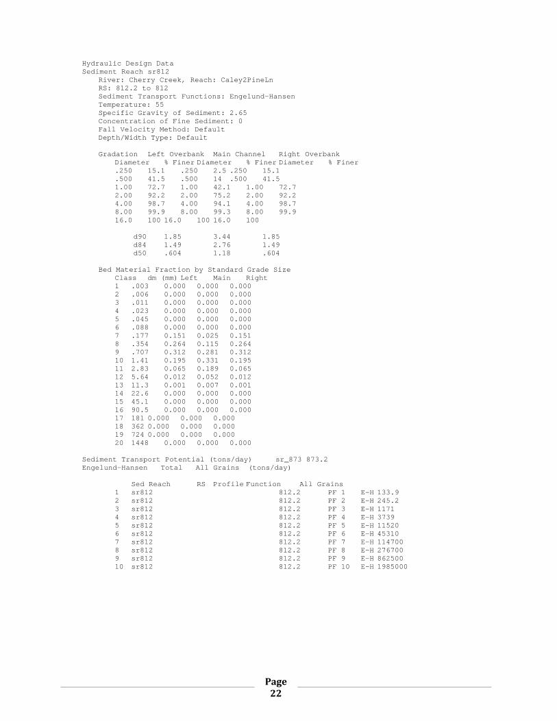
Page 22
Hydraulic Design Data Sediment Reach sr812 River: Cherry Creek, Reach: Caley2PineLn RS: 812.2 to 812 Sediment Transport Functions: Engelund-Hansen Temperature: 55 Specific Gravity of Sediment: 2.65 Concentration of Fine Sediment: 0 Fall Velocity Method: Default Depth/Width Type: Default Gradation Left Overbank Main Channel Right Overbank Diameter % Finer Diameter % Finer Diameter % Finer .250 15.1 .250 2.5 .250 15.1 .500 41.5 .500 14 .500 41.5 1.00 72.7 1.00 42.1 1.00 72.7 2.00 92.2 2.00 75.2 2.00 92.2 4.00 98.7 4.00 94.1 4.00 98.7 8.00 99.9 8.00 99.3 8.00 99.9 16.0 100 16.0 100 16.0 100 d90 1.85 3.44 1.85 d84 1.49 2.76 1.49 d50 .604 1.18 .604 Bed Material Fraction by Standard Grade Size Class dm (mm) Left Main Right 1 .003 0.000 0.000 0.000 2 .006 0.000 0.000 0.000 3 .011 0.000 0.000 0.000 4 .023 0.000 0.000 0.000 5 .045 0.000 0.000 0.000 6 .088 0.000 0.000 0.000 7 .177 0.151 0.025 0.151 8 .354 0.264 0.115 0.264 9 .707 0.312 0.281 0.312 10 1.41 0.195 0.331 0.195 11 2.83 0.065 0.189 0.065 12 5.64 0.012 0.052 0.012 13 11.3 0.001 0.007 0.001 14 22.6 0.000 0.000 0.000 15 45.1 0.000 0.000 0.000 16 90.5 0.000 0.000 0.000 17 181 0.000 0.000 0.000 18 362 0.000 0.000 0.000 19 724 0.000 0.000 0.000 20 1448 0.000 0.000 0.000
Sediment Transport Potential (tons/day) sr_873 873.2 Engelund-Hansen Total All Grains (tons/day) Sed Reach RS Profile Function All Grains 1 sr812 812.2 PF 1 E-H 133.9 2 sr812 812.2 PF 2 E-H 245.2 3 sr812 812.2 PF 3 E-H 1171 4 sr812 812.2 PF 4 E-H 3739 5 sr812 812.2 PF 5 E-H 11520 6 sr812 812.2 PF 6 E-H 45310 7 sr812 812.2 PF 7 E-H 114700 8 sr812 812.2 PF 8 E-H 276700 9 sr812 812.2 PF 9 E-H 862500 10 sr812 812.2 PF 10 E-H 1985000

Page 23
Hydraulic Design Data Sediment Reach sr813 River: Cherry Creek, Reach: Caley2PineLn RS: 813.2 to 813.2 Sediment Transport Functions: Engelund-Hansen Temperature: 55 Specific Gravity of Sediment: 2.65 Concentration of Fine Sediment: 0 Fall Velocity Method: Default Depth/Width Type: Default Gradation Left Overbank Main Channel Right Overbank Diameter % Finer Diameter % Finer Diameter % Finer .250 15.1 .250 2.5 .250 15.1 .500 41.5 .500 14 .500 41.5 1.00 72.7 1.00 42.1 1.00 72.7 2.00 92.2 2.00 75.2 2.00 92.2 4.00 98.7 4.00 94.1 4.00 98.7 8.00 99.9 8.00 99.3 8.00 99.9 16.0 100 16.0 100 16.0 100 d90 1.85 3.44 1.85 d84 1.49 2.76 1.49 d50 .604 1.18 .604 Bed Material Fraction by Standard Grade Size Class dm (mm) Left Main Right 1 .003 0.000 0.000 0.000 2 .006 0.000 0.000 0.000 3 .011 0.000 0.000 0.000 4 .023 0.000 0.000 0.000 5 .045 0.000 0.000 0.000 6 .088 0.000 0.000 0.000 7 .177 0.151 0.025 0.151 8 .354 0.264 0.115 0.264 9 .707 0.312 0.281 0.312 10 1.41 0.195 0.331 0.195 11 2.83 0.065 0.189 0.065 12 5.64 0.012 0.052 0.012 13 11.3 0.001 0.007 0.001 14 22.6 0.000 0.000 0.000 15 45.1 0.000 0.000 0.000 16 90.5 0.000 0.000 0.000 17 181 0.000 0.000 0.000 18 362 0.000 0.000 0.000 19 724 0.000 0.000 0.000 20 1448 0.000 0.000 0.000 Sediment Transport Potential (tons/day) (tons/day) Sed Reach RS Profile Function All Grains 1 sr813 813.2 PF 1 E-H 65.11 2 sr813 813.2 PF 2 E-H 126.6 3 sr813 813.2 PF 3 E-H 563.8 4 sr813 813.2 PF 4 E-H 1813 5 sr813 813.2 PF 5 E-H 5327 6 sr813 813.2 PF 6 E-H 18150 7 sr813 813.2 PF 7 E-H 35070 8 sr813 813.2 PF 8 E-H 74900 9 sr813 813.2 PF 9 E-H 169000 10 sr813 813.2 PF 10 E-H 357300
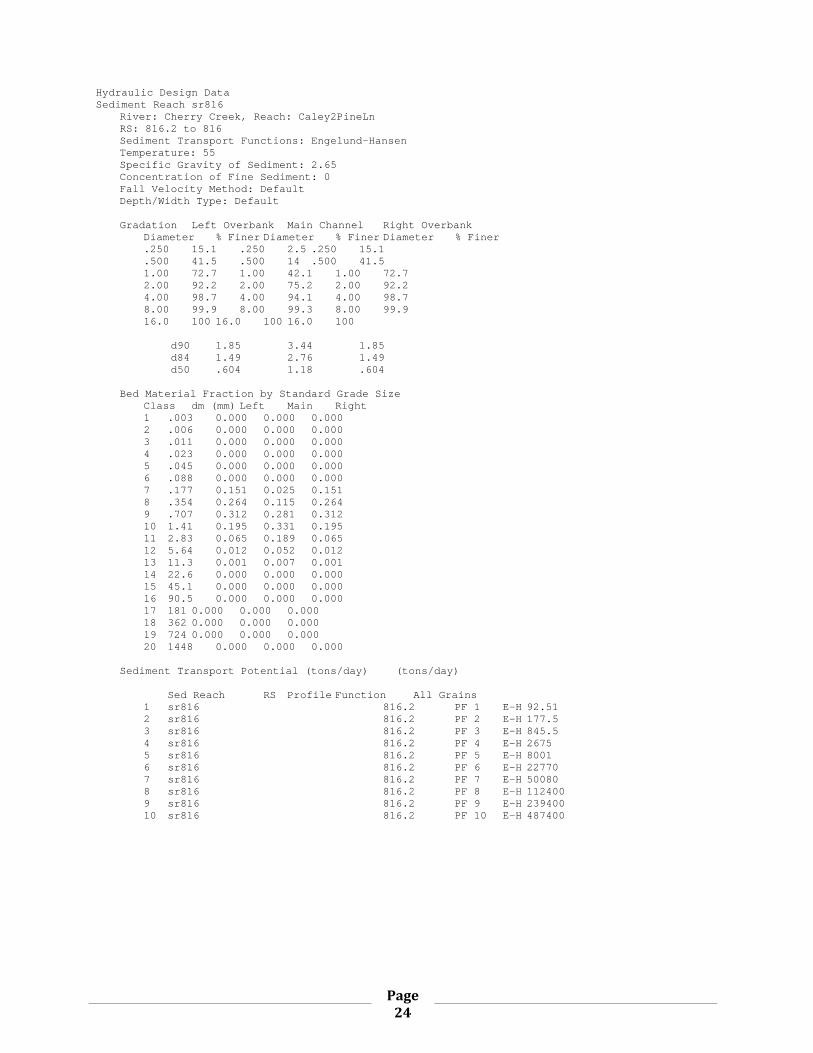
Page 24
Hydraulic Design Data Sediment Reach sr816 River: Cherry Creek, Reach: Caley2PineLn RS: 816.2 to 816 Sediment Transport Functions: Engelund-Hansen Temperature: 55 Specific Gravity of Sediment: 2.65 Concentration of Fine Sediment: 0 Fall Velocity Method: Default Depth/Width Type: Default Gradation Left Overbank Main Channel Right Overbank Diameter % Finer Diameter % Finer Diameter % Finer .250 15.1 .250 2.5 .250 15.1 .500 41.5 .500 14 .500 41.5 1.00 72.7 1.00 42.1 1.00 72.7 2.00 92.2 2.00 75.2 2.00 92.2 4.00 98.7 4.00 94.1 4.00 98.7 8.00 99.9 8.00 99.3 8.00 99.9 16.0 100 16.0 100 16.0 100 d90 1.85 3.44 1.85 d84 1.49 2.76 1.49 d50 .604 1.18 .604 Bed Material Fraction by Standard Grade Size Class dm (mm) Left Main Right 1 .003 0.000 0.000 0.000 2 .006 0.000 0.000 0.000 3 .011 0.000 0.000 0.000 4 .023 0.000 0.000 0.000 5 .045 0.000 0.000 0.000 6 .088 0.000 0.000 0.000 7 .177 0.151 0.025 0.151 8 .354 0.264 0.115 0.264 9 .707 0.312 0.281 0.312 10 1.41 0.195 0.331 0.195 11 2.83 0.065 0.189 0.065 12 5.64 0.012 0.052 0.012 13 11.3 0.001 0.007 0.001 14 22.6 0.000 0.000 0.000 15 45.1 0.000 0.000 0.000 16 90.5 0.000 0.000 0.000 17 181 0.000 0.000 0.000 18 362 0.000 0.000 0.000 19 724 0.000 0.000 0.000 20 1448 0.000 0.000 0.000 Sediment Transport Potential (tons/day) (tons/day) Sed Reach RS Profile Function All Grains 1 sr816 816.2 PF 1 E-H 92.51 2 sr816 816.2 PF 2 E-H 177.5 3 sr816 816.2 PF 3 E-H 845.5 4 sr816 816.2 PF 4 E-H 2675 5 sr816 816.2 PF 5 E-H 8001 6 sr816 816.2 PF 6 E-H 22770 7 sr816 816.2 PF 7 E-H 50080 8 sr816 816.2 PF 8 E-H 112400 9 sr816 816.2 PF 9 E-H 239400 10 sr816 816.2 PF 10 E-H 487400

Page 25
Hydraulic Design Data Sediment Reach sr819 River: Cherry Creek, Reach: Caley2PineLn RS: 819.2 to 819 Sediment Transport Functions: Engelund-Hansen Temperature: 55 Specific Gravity of Sediment: 2.65 Concentration of Fine Sediment: 0 Fall Velocity Method: Default Depth/Width Type: Default Gradation Left Overbank Main Channel Right Overbank Diameter % Finer Diameter % Finer Diameter % Finer .250 15.1 .250 2.5 .250 15.1 .500 41.5 .500 14 .500 41.5 1.00 72.7 1.00 42.1 1.00 72.7 2.00 92.2 2.00 75.2 2.00 92.2 4.00 98.7 4.00 94.1 4.00 98.7 8.00 99.9 8.00 99.3 8.00 99.9 16.0 100 16.0 100 16.0 100 d90 1.85 3.44 1.85 d84 1.49 2.76 1.49 d50 .604 1.18 .604 Bed Material Fraction by Standard Grade Size Class dm (mm) Left Main Right 1 .003 0.000 0.000 0.000 2 .006 0.000 0.000 0.000 3 .011 0.000 0.000 0.000 4 .023 0.000 0.000 0.000 5 .045 0.000 0.000 0.000 6 .088 0.000 0.000 0.000 7 .177 0.151 0.025 0.151 8 .354 0.264 0.115 0.264 9 .707 0.312 0.281 0.312 10 1.41 0.195 0.331 0.195 11 2.83 0.065 0.189 0.065 12 5.64 0.012 0.052 0.012 13 11.3 0.001 0.007 0.001 14 22.6 0.000 0.000 0.000 15 45.1 0.000 0.000 0.000 16 90.5 0.000 0.000 0.000 17 181 0.000 0.000 0.000 18 362 0.000 0.000 0.000 19 724 0.000 0.000 0.000 20 1448 0.000 0.000 0.000 Sediment Transport Potential (tons/day) sr_873 873.2
Engelund-Hansen Total All Grains (tons/day) Sed Reach RS Profile Function All Grains 1 sr819 819.2 PF 1 E-H 99.45 2 sr819 819.2 PF 2 E-H 160.5 3 sr819 819.2 PF 3 E-H 758.9 4 sr819 819.2 PF 4 E-H 2484 5 sr819 819.2 PF 5 E-H 7019 6 sr819 819.2 PF 6 E-H 29820 7 sr819 819.2 PF 7 E-H 78020 8 sr819 819.2 PF 8 E-H 183300 9 sr819 819.2 PF 9 E-H 612400 10 sr819 819.2 PF 10 E-H 1608000

Page 26
Hydraulic Design Data Sediment Reach sr821 River: Cherry Creek, Reach: Caley2PineLn RS: 821.2 to 821 Sediment Transport Functions: Engelund-Hansen Temperature: 55 Specific Gravity of Sediment: 2.65 Concentration of Fine Sediment: 0 Fall Velocity Method: Default Depth/Width Type: Default Gradation Left Overbank Main Channel Right Overbank Diameter % Finer Diameter % Finer Diameter % Finer .250 15.1 .250 2.5 .250 15.1 .500 41.5 .500 14 .500 41.5 1.00 72.7 1.00 42.1 1.00 72.7 2.00 92.2 2.00 75.2 2.00 92.2 4.00 98.7 4.00 94.1 4.00 98.7 8.00 99.9 8.00 99.3 8.00 99.9 16.0 100 16.0 100 16.0 100 d90 1.85 3.44 1.85 d84 1.49 2.76 1.49 d50 .604 1.18 .604 Bed Material Fraction by Standard Grade Size Class dm (mm) Left Main Right 1 .003 0.000 0.000 0.000 2 .006 0.000 0.000 0.000 3 .011 0.000 0.000 0.000 4 .023 0.000 0.000 0.000 5 .045 0.000 0.000 0.000 6 .088 0.000 0.000 0.000 7 .177 0.151 0.025 0.151 8 .354 0.264 0.115 0.264 9 .707 0.312 0.281 0.312 10 1.41 0.195 0.331 0.195 11 2.83 0.065 0.189 0.065 12 5.64 0.012 0.052 0.012 13 11.3 0.001 0.007 0.001 14 22.6 0.000 0.000 0.000 15 45.1 0.000 0.000 0.000 16 90.5 0.000 0.000 0.000 17 181 0.000 0.000 0.000 18 362 0.000 0.000 0.000 19 724 0.000 0.000 0.000 20 1448 0.000 0.000 0.000 Sediment Transport Potential (tons/day) (tons/day) Sed Reach RS Profile Function All Grains 1 sr821 821.2 PF 1 E-H 75.20 2 sr821 821.2 PF 2 E-H 116.3 3 sr821 821.2 PF 3 E-H 553.5 4 sr821 821.2 PF 4 E-H 1854 5 sr821 821.2 PF 5 E-H 6125 6 sr821 821.2 PF 6 E-H 19830 7 sr821 821.2 PF 7 E-H 44690 8 sr821 821.2 PF 8 E-H 93610 9 sr821 821.2 PF 9 E-H 227600 10 sr821 821.2 PF 10 E-H 504600

Page 27
Hydraulic Design Data Sediment Reach sr_867 River: Cherry Creek, Reach: Caley2PineLn RS: 867.2 to 867 Sediment Transport Functions: Engelund-Hansen Temperature: 55 Specific Gravity of Sediment: 2.65 Concentration of Fine Sediment: 0 Fall Velocity Method: Default Depth/Width Type: Default Gradation Left Overbank Main Channel Right Overbank Diameter % Finer Diameter % Finer Diameter % Finer .250 15.1 .250 2.5 .250 15.1 .500 41.5 .500 14 .500 41.5 1.00 72.7 1.00 42.1 1.00 72.7 2.00 92.2 2.00 75.2 2.00 92.2 4.00 98.7 4.00 94.1 4.00 98.7 8.00 99.9 8.00 99.3 8.00 99.9 16.0 100 16.0 100 16.0 100 d90 1.85 3.44 1.85 d84 1.49 2.76 1.49 d50 .604 1.18 .604 Bed Material Fraction by Standard Grade Size Class dm (mm) Left Main Right 1 .003 0.000 0.000 0.000 2 .006 0.000 0.000 0.000 3 .011 0.000 0.000 0.000 4 .023 0.000 0.000 0.000 5 .045 0.000 0.000 0.000 6 .088 0.000 0.000 0.000 7 .177 0.151 0.025 0.151 8 .354 0.264 0.115 0.264 9 .707 0.312 0.281 0.312 10 1.41 0.195 0.331 0.195 11 2.83 0.065 0.189 0.065 12 5.64 0.012 0.052 0.012 13 11.3 0.001 0.007 0.001 14 22.6 0.000 0.000 0.000 15 45.1 0.000 0.000 0.000 16 90.5 0.000 0.000 0.000 17 181 0.000 0.000 0.000 18 362 0.000 0.000 0.000 19 724 0.000 0.000 0.000 20 1448 0.000 0.000 0.000 Sediment Transport Potential (tons/day) sr_873 873.2
Engelund-Hansen Total All Grains (tons/day) Sed Reach RS Profile Function All Grains 1 sr_867 867.2 PF 1 E-H 220.0 2 sr_867 867.2 PF 2 E-H 245.4 3 sr_867 867.2 PF 3 E-H 1178 4 sr_867 867.2 PF 4 E-H 3651 5 sr_867 867.2 PF 5 E-H 11680 6 sr_867 867.2 PF 6 E-H 51720 7 sr_867 867.2 PF 7 E-H 122600 8 sr_867 867.2 PF 8 E-H 169600 9 sr_867 867.2 PF 9 E-H 700500 10 sr_867 867.2 PF 10 E-H 1596000

Page 28
Hydraulic Design Data Sediment Reach sr_868 River: Cherry Creek, Reach: Caley2PineLn RS: 868.2 to 868 Sediment Transport Functions: Engelund-Hansen Temperature: 55 Specific Gravity of Sediment: 2.65 Concentration of Fine Sediment: 0 Fall Velocity Method: Default Depth/Width Type: Default Gradation Left Overbank Main Channel Right Overbank Diameter % Finer Diameter % Finer Diameter % Finer .250 15.1 .250 2.5 .250 15.1 .500 41.5 .500 14 .500 41.5 1.00 72.7 1.00 42.1 1.00 72.7 2.00 92.2 2.00 75.2 2.00 92.2 4.00 98.7 4.00 94.1 4.00 98.7 8.00 99.9 8.00 99.3 8.00 99.9 16.0 100 16.0 100 16.0 100 d90 1.85 3.44 1.85 d84 1.49 2.76 1.49 d50 .604 1.18 .604 Bed Material Fraction by Standard Grade Size Class dm (mm) Left Main Right 1 .003 0.000 0.000 0.000 2 .006 0.000 0.000 0.000 3 .011 0.000 0.000 0.000 4 .023 0.000 0.000 0.000 5 .045 0.000 0.000 0.000 6 .088 0.000 0.000 0.000 7 .177 0.151 0.025 0.151 8 .354 0.264 0.115 0.264 9 .707 0.312 0.281 0.312 10 1.41 0.195 0.331 0.195 11 2.83 0.065 0.189 0.065 12 5.64 0.012 0.052 0.012 13 11.3 0.001 0.007 0.001 14 22.6 0.000 0.000 0.000 15 45.1 0.000 0.000 0.000 16 90.5 0.000 0.000 0.000 17 181 0.000 0.000 0.000 18 362 0.000 0.000 0.000 19 724 0.000 0.000 0.000 20 1448 0.000 0.000 0.000 Sediment Transport Potential (tons/day) sr_873 873.2
Engelund-Hansen Total All Grains (tons/day) Sed Reach RS Profile Function All Grains 1 sr_868 868.2 PF 1 E-H 66.99 2 sr_868 868.2 PF 2 E-H 207.3 3 sr_868 868.2 PF 3 E-H 990.3 4 sr_868 868.2 PF 4 E-H 3152 5 sr_868 868.2 PF 5 E-H 10060 6 sr_868 868.2 PF 6 E-H 43100 7 sr_868 868.2 PF 7 E-H 123600 8 sr_868 868.2 PF 8 E-H 318400 9 sr_868 868.2 PF 9 E-H 635000 10 sr_868 868.2 PF 10 E-H 1102000

Page 29
Hydraulic Design Data Sediment Reach sr_869 River: Cherry Creek, Reach: Caley2PineLn RS: 867.2 to 867 Sediment Transport Functions: Engelund-Hansen Temperature: 55 Specific Gravity of Sediment: 2.65 Concentration of Fine Sediment: 0 Fall Velocity Method: Default Depth/Width Type: Default Gradation Left Overbank Main Channel Right Overbank Diameter % Finer Diameter % Finer Diameter % Finer .250 15.1 .250 2.5 .250 15.1 .500 41.5 .500 14 .500 41.5 1.00 72.7 1.00 42.1 1.00 72.7 2.00 92.2 2.00 75.2 2.00 92.2 4.00 98.7 4.00 94.1 4.00 98.7 8.00 99.9 8.00 99.3 8.00 99.9 16.0 100 16.0 100 16.0 100 d90 1.85 3.44 1.85 d84 1.49 2.76 1.49 d50 .604 1.18 .604 Bed Material Fraction by Standard Grade Size Class dm (mm) Left Main Right 1 .003 0.000 0.000 0.000 2 .006 0.000 0.000 0.000 3 .011 0.000 0.000 0.000 4 .023 0.000 0.000 0.000 5 .045 0.000 0.000 0.000 6 .088 0.000 0.000 0.000 7 .177 0.151 0.025 0.151 8 .354 0.264 0.115 0.264 9 .707 0.312 0.281 0.312 10 1.41 0.195 0.331 0.195 11 2.83 0.065 0.189 0.065 12 5.64 0.012 0.052 0.012 13 11.3 0.001 0.007 0.001 14 22.6 0.000 0.000 0.000 15 45.1 0.000 0.000 0.000 16 90.5 0.000 0.000 0.000 17 181 0.000 0.000 0.000 18 362 0.000 0.000 0.000 19 724 0.000 0.000 0.000 20 1448 0.000 0.000 0.000 Sediment Transport Potential (tons/day) sr_869 869.2
Engelund-Hansen Total All Grains (tons/day) Sed Reach RS Profile Function All Grains 1 sr_869 867.2 PF 1 E-H 177.5 2 sr_869 867.2 PF 2 E-H 230.8 3 sr_869 867.2 PF 3 E-H 1059 4 sr_869 867.2 PF 4 E-H 3219 5 sr_869 867.2 PF 5 E-H 9803 6 sr_869 867.2 PF 6 E-H 40910 7 sr_869 867.2 PF 7 E-H 98910 8 sr_869 867.2 PF 8 E-H 217500 9 sr_869 867.2 PF 9 E-H 673300 10 sr_869 867.2 PF 10 E-H 1661000
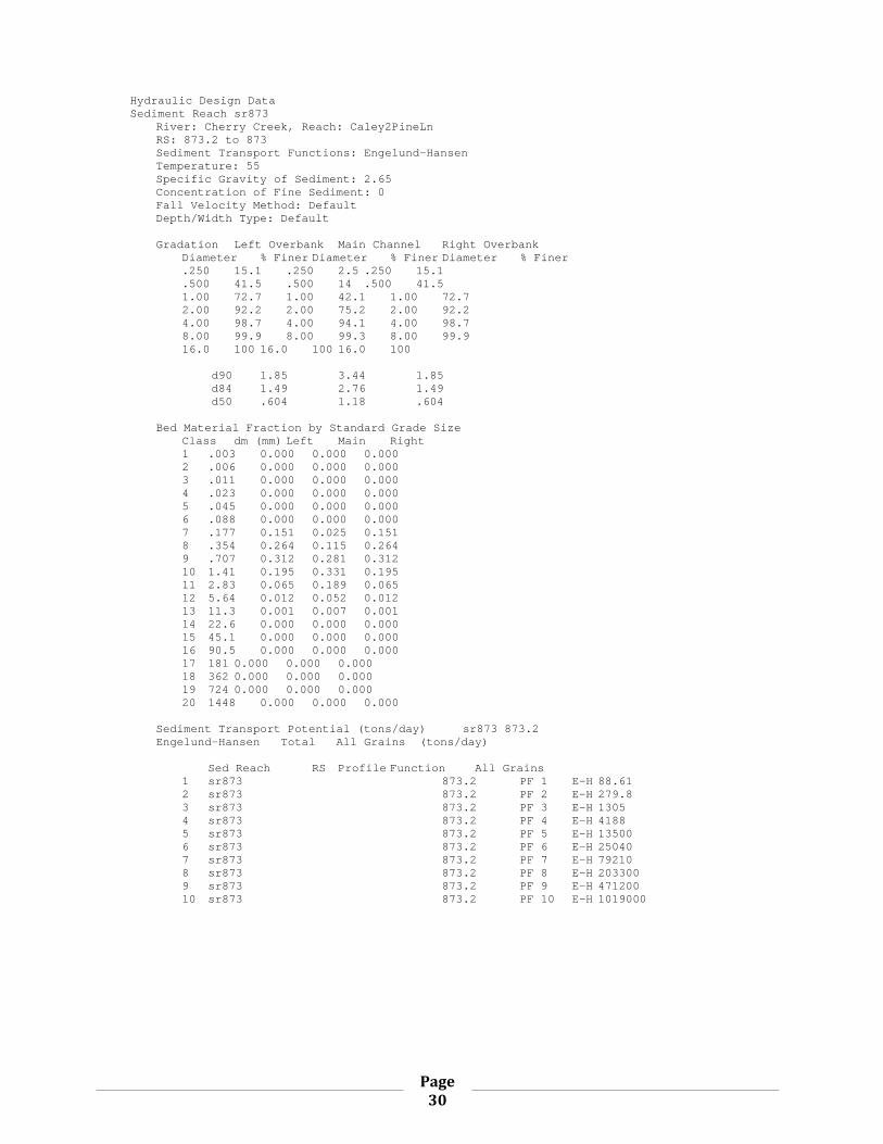
Page 30
Hydraulic Design Data Sediment Reach sr873 River: Cherry Creek, Reach: Caley2PineLn RS: 873.2 to 873 Sediment Transport Functions: Engelund-Hansen Temperature: 55 Specific Gravity of Sediment: 2.65 Concentration of Fine Sediment: 0 Fall Velocity Method: Default Depth/Width Type: Default Gradation Left Overbank Main Channel Right Overbank Diameter % Finer Diameter % Finer Diameter % Finer .250 15.1 .250 2.5 .250 15.1 .500 41.5 .500 14 .500 41.5 1.00 72.7 1.00 42.1 1.00 72.7 2.00 92.2 2.00 75.2 2.00 92.2 4.00 98.7 4.00 94.1 4.00 98.7 8.00 99.9 8.00 99.3 8.00 99.9 16.0 100 16.0 100 16.0 100 d90 1.85 3.44 1.85 d84 1.49 2.76 1.49 d50 .604 1.18 .604 Bed Material Fraction by Standard Grade Size Class dm (mm) Left Main Right 1 .003 0.000 0.000 0.000 2 .006 0.000 0.000 0.000 3 .011 0.000 0.000 0.000 4 .023 0.000 0.000 0.000 5 .045 0.000 0.000 0.000 6 .088 0.000 0.000 0.000 7 .177 0.151 0.025 0.151 8 .354 0.264 0.115 0.264 9 .707 0.312 0.281 0.312 10 1.41 0.195 0.331 0.195 11 2.83 0.065 0.189 0.065 12 5.64 0.012 0.052 0.012 13 11.3 0.001 0.007 0.001 14 22.6 0.000 0.000 0.000 15 45.1 0.000 0.000 0.000 16 90.5 0.000 0.000 0.000 17 181 0.000 0.000 0.000 18 362 0.000 0.000 0.000 19 724 0.000 0.000 0.000 20 1448 0.000 0.000 0.000 Sediment Transport Potential (tons/day) sr873 873.2
Engelund-Hansen Total All Grains (tons/day) Sed Reach RS Profile Function All Grains 1 sr873 873.2 PF 1 E-H 88.61 2 sr873 873.2 PF 2 E-H 279.8 3 sr873 873.2 PF 3 E-H 1305 4 sr873 873.2 PF 4 E-H 4188 5 sr873 873.2 PF 5 E-H 13500 6 sr873 873.2 PF 6 E-H 25040 7 sr873 873.2 PF 7 E-H 79210 8 sr873 873.2 PF 8 E-H 203300 9 sr873 873.2 PF 9 E-H 471200 10 sr873 873.2 PF 10 E-H 1019000

Page 31
Hydraulic Design Data Sediment Reach sr_878 River: Cherry Creek, Reach: Caley2PineLn RS: 878.2 to 878 Sediment Transport Functions: Engelund-Hansen Temperature: 55 Specific Gravity of Sediment: 2.65 Concentration of Fine Sediment: 0 Fall Velocity Method: Default Depth/Width Type: Default Gradation Left Overbank Main Channel Right Overbank Diameter % Finer Diameter % Finer Diameter % Finer .250 15.1 .250 2.5 .250 15.1 .500 41.5 .500 14 .500 41.5 1.00 72.7 1.00 42.1 1.00 72.7 2.00 92.2 2.00 75.2 2.00 92.2 4.00 98.7 4.00 94.1 4.00 98.7 8.00 99.9 8.00 99.3 8.00 99.9 16.0 100 16.0 100 16.0 100 d90 1.85 3.44 1.85 d84 1.49 2.76 1.49 d50 .604 1.18 .604 Bed Material Fraction by Standard Grade Size Class dm (mm) Left Main Right 1 .003 0.000 0.000 0.000 2 .006 0.000 0.000 0.000 3 .011 0.000 0.000 0.000 4 .023 0.000 0.000 0.000 5 .045 0.000 0.000 0.000 6 .088 0.000 0.000 0.000 7 .177 0.151 0.025 0.151 8 .354 0.264 0.115 0.264 9 .707 0.312 0.281 0.312 10 1.41 0.195 0.331 0.195 11 2.83 0.065 0.189 0.065 12 5.64 0.012 0.052 0.012 13 11.3 0.001 0.007 0.001 14 22.6 0.000 0.000 0.000 15 45.1 0.000 0.000 0.000 16 90.5 0.000 0.000 0.000 17 181 0.000 0.000 0.000 18 362 0.000 0.000 0.000 19 724 0.000 0.000 0.000 20 1448 0.000 0.000 0.000 Sediment Transport Potential (tons/day) sedRch 880.2
Engelund-Hansen Total All Grains (tons/day) Sed Reach RS Profile Function All Grains 1 sr_878 878.2 PF 1 E-H 164.5 2 sr_878 878.2 PF 2 E-H 393.3 3 sr_878 878.2 PF 3 E-H 915.9 4 sr_878 878.2 PF 4 E-H 3216 5 sr_878 878.2 PF 5 E-H 10040 6 sr_878 878.2 PF 6 E-H 38510 7 sr_878 878.2 PF 7 E-H 101500 8 sr_878 878.2 PF 8 E-H 198300 9 sr_878 878.2 PF 9 E-H 459600 10 sr_878 878.2 PF 10 E-H 835900

Page 32
Hydraulic Design Data Sediment Reach sedRch River: Cherry Creek, Reach: Caley2PineLn RS: 880.2 to 880.2 Sediment Transport Functions: Engelund-Hansen Temperature: 55 Specific Gravity of Sediment: 2.65 Concentration of Fine Sediment: 0 Fall Velocity Method: Default Depth/Width Type: Default Gradation Left Overbank Main Channel Right Overbank Diameter % Finer Diameter % Finer Diameter % Finer .250 15.1 .250 2.5 .250 15.1 .500 41.5 .500 14 .500 41.5 1.00 72.7 1.00 42.1 1.00 72.7 2.00 92.2 2.00 75.2 2.00 92.2 4.00 98.7 4.00 94.1 4.00 98.7 8.00 99.9 8.00 99.3 8.00 99.9 16.0 100 16.0 100 16.0 100 d90 1.85 3.44 1.85 d84 1.49 2.76 1.49 d50 .604 1.18 .604 Bed Material Fraction by Standard Grade Size Class dm (mm) Left Main Right 1 .003 0.000 0.000 0.000 2 .006 0.000 0.000 0.000 3 .011 0.000 0.000 0.000 4 .023 0.000 0.000 0.000 5 .045 0.000 0.000 0.000 6 .088 0.000 0.000 0.000 7 .177 0.151 0.025 0.151 8 .354 0.264 0.115 0.264 9 .707 0.312 0.281 0.312 10 1.41 0.195 0.331 0.195 11 2.83 0.065 0.189 0.065 12 5.64 0.012 0.052 0.012 13 11.3 0.001 0.007 0.001 14 22.6 0.000 0.000 0.000 15 45.1 0.000 0.000 0.000 16 90.5 0.000 0.000 0.000 17 181 0.000 0.000 0.000 18 362 0.000 0.000 0.000 19 724 0.000 0.000 0.000 20 1448 0.000 0.000 0.000 Sediment Transport Potential (tons/day) sedRch 880.2
Engelund-Hansen Total All Grains (tons/day) Sed Reach RS Profile Function All Grains 1 sedRch 880.2 PF 1 E-H 100.3 2 sedRch 880.2 PF 2 E-H 321.1 3 sedRch 880.2 PF 3 E-H 1428 4 sedRch 880.2 PF 4 E-H 4191 5 sedRch 880.2 PF 5 E-H 10700 6 sedRch 880.2 PF 6 E-H 30290 7 sedRch 880.2 PF 7 E-H 56710 8 sedRch 880.2 PF 8 E-H 93280 9 sedRch 880.2 PF 9 E-H 188800 10 sedRch 880.2 PF 10 E-H 367900

APPENDIX C . SUB-REACH FLOW DATA FROM CCBWQA MODEL
Sub-Segment Stream Flows (monthly volume - ac-ft) (Third period of CCBWQA model)
880 878 873 869 867 868 819 816 821 813 812 811Inc. Length (ft) 2180 1715 5270 1032 2615 696 2353 5657 2903 1378 627 70Total Q (ac-ft) 76368 74567 72358 67681 65061 65718 70918 61328 62880 59287 56555 52232
Total L (mi) 5.0 4.6 4.3 3.3 3.1 2.6 2.5 2.0 0.9 0.4 0.1 0.0Jan‐95 0.2 0.2 0.2 0.2 0.2 0.2 0.1 0.0 0.0 0.0 0.0 0.0Feb‐95 41.9 36.0 29.8 41.3 30.9 22.3 1.7 0.0 0.0 0.0 0.0 0.0Mar‐95 136.7 130.9 124.9 122.8 108.4 102.4 104.9 74.9 74.9 64.4 55.8 45.0Apr‐95 198.1 171.7 159.6 157.8 144.0 144.5 155.6 129.5 135.2 134.0 127.2 109.6May‐95 640.1 653.3 664.9 619.3 610.8 632.0 758.7 672.2 706.7 687.2 658.7 594.9Jun‐95 2176.2 2160.6 2159.9 2005.2 1976.2 2010.1 2461.2 2315.1 2373.0 2328.7 2277.3 2146.1Jul‐95 1921.1 1867.9 1848.0 1724.0 1707.8 1746.3 2158.7 2043.8 2108.7 2076.5 2027.7 1903.8Aug‐95 1060.2 1047.4 1027.9 928.5 900.2 914.4 969.6 877.7 902.4 876.1 842.6 772.5Sep‐95 419.6 380.5 314.1 303.0 294.5 303.0 389.7 358.6 376.8 375.5 365.7 336.9Oct‐95 836.5 809.3 777.1 722.9 684.3 695.3 917.0 827.8 851.8 826.2 773.5 687.0Nov‐95 280.4 275.0 264.4 261.8 272.6 271.6 253.1 224.7 230.8 221.0 232.9 239.8Dec‐95 176.3 175.7 172.9 172.2 157.9 159.9 115.2 54.1 57.2 52.3 41.5 28.9Jan‐96 71.1 69.5 71.5 83.7 74.0 67.9 18.4 9.9 9.9 8.4 12.0 11.4Feb‐96 50.8 49.2 46.8 57.9 47.2 38.6 0.0 0.0 0.0 0.0 0.0 0.0Mar‐96 72.8 69.4 65.2 74.8 64.8 58.9 25.1 0.0 0.0 0.0 0.0 0.0Apr‐96 228.2 216.6 199.4 207.9 203.1 208.3 214.0 94.7 104.8 88.6 86.3 77.7May‐96 56.7 41.0 23.5 37.5 32.0 33.0 45.0 28.5 34.7 34.9 35.0 29.0Jun‐96 545.2 515.2 471.7 451.6 436.5 440.8 582.9 550.8 562.2 545.0 529.2 497.0Jul‐96 449.2 423.6 392.7 385.6 373.5 375.9 443.2 429.6 437.9 432.3 422.9 402.8Aug‐96 125.0 113.5 75.6 84.4 73.1 73.5 112.0 93.1 98.3 94.2 87.8 76.9Sep‐96 393.6 359.5 263.8 245.4 235.7 244.3 364.6 330.4 348.9 344.1 333.8 305.6Oct‐96 490.7 455.4 379.6 358.6 361.7 384.5 634.3 605.8 647.0 646.6 635.3 587.2Nov‐96 110.9 93.7 68.2 75.5 63.6 62.5 114.8 104.3 107.5 102.0 97.0 88.3Dec‐96 35.5 0.0 0.0 15.3 5.0 1.9 0.0 0.0 0.0 0.0 0.0 0.0
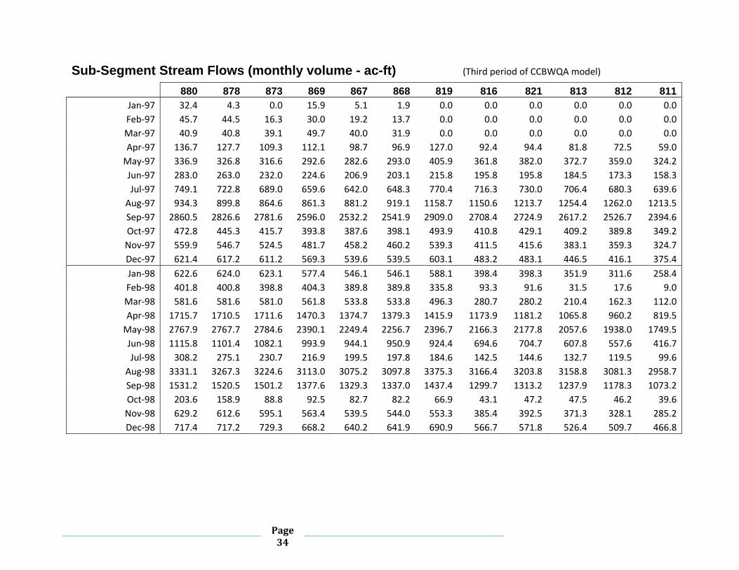
Page 34
Sub-Segment Stream Flows (monthly volume - ac-ft) (Third period of CCBWQA model)
880 878 873 869 867 868 819 816 821 813 812 811Jan‐97 32.4 4.3 0.0 15.9 5.1 1.9 0.0 0.0 0.0 0.0 0.0 0.0Feb‐97 45.7 44.5 16.3 30.0 19.2 13.7 0.0 0.0 0.0 0.0 0.0 0.0Mar‐97 40.9 40.8 39.1 49.7 40.0 31.9 0.0 0.0 0.0 0.0 0.0 0.0Apr‐97 136.7 127.7 109.3 112.1 98.7 96.9 127.0 92.4 94.4 81.8 72.5 59.0May‐97 336.9 326.8 316.6 292.6 282.6 293.0 405.9 361.8 382.0 372.7 359.0 324.2Jun‐97 283.0 263.0 232.0 224.6 206.9 203.1 215.8 195.8 195.8 184.5 173.3 158.3Jul‐97 749.1 722.8 689.0 659.6 642.0 648.3 770.4 716.3 730.0 706.4 680.3 639.6Aug‐97 934.3 899.8 864.6 861.3 881.2 919.1 1158.7 1150.6 1213.7 1254.4 1262.0 1213.5Sep‐97 2860.5 2826.6 2781.6 2596.0 2532.2 2541.9 2909.0 2708.4 2724.9 2617.2 2526.7 2394.6Oct‐97 472.8 445.3 415.7 393.8 387.6 398.1 493.9 410.8 429.1 409.2 389.8 349.2Nov‐97 559.9 546.7 524.5 481.7 458.2 460.2 539.3 411.5 415.6 383.1 359.3 324.7Dec‐97 621.4 617.2 611.2 569.3 539.6 539.5 603.1 483.2 483.1 446.5 416.1 375.4Jan‐98 622.6 624.0 623.1 577.4 546.1 546.1 588.1 398.4 398.3 351.9 311.6 258.4Feb‐98 401.8 400.8 398.8 404.3 389.8 389.8 335.8 93.3 91.6 31.5 17.6 9.0Mar‐98 581.6 581.6 581.0 561.8 533.8 533.8 496.3 280.7 280.2 210.4 162.3 112.0Apr‐98 1715.7 1710.5 1711.6 1470.3 1374.7 1379.3 1415.9 1173.9 1181.2 1065.8 960.2 819.5May‐98 2767.9 2767.7 2784.6 2390.1 2249.4 2256.7 2396.7 2166.3 2177.8 2057.6 1938.0 1749.5Jun‐98 1115.8 1101.4 1082.1 993.9 944.1 950.9 924.4 694.6 704.7 607.8 557.6 416.7Jul‐98 308.2 275.1 230.7 216.9 199.5 197.8 184.6 142.5 144.6 132.7 119.5 99.6Aug‐98 3331.1 3267.3 3224.6 3113.0 3075.2 3097.8 3375.3 3166.4 3203.8 3158.8 3081.3 2958.7Sep‐98 1531.2 1520.5 1501.2 1377.6 1329.3 1337.0 1437.4 1299.7 1313.2 1237.9 1178.3 1073.2Oct‐98 203.6 158.9 88.8 92.5 82.7 82.2 66.9 43.1 47.2 47.5 46.2 39.6Nov‐98 629.2 612.6 595.1 563.4 539.5 544.0 553.3 385.4 392.5 371.3 328.1 285.2Dec‐98 717.4 717.2 729.3 668.2 640.2 641.9 690.9 566.7 571.8 526.4 509.7 466.8

Page 35
Sub-Segment Stream Flows (monthly volumes - ac-ft) (Third period of CCBWQA model)
880 878 873 869 867 868 819 816 821 813 812 811Jan‐99 905.9 907.3 918.5 869.3 837.2 837.2 806.9 564.4 563.2 480.3 429.9 390.8Feb‐99 613.5 614.2 613.3 589.5 564.7 564.7 533.4 289.9 289.5 193.1 150.2 114.0Mar‐99 654.7 655.3 657.5 644.1 625.1 625.1 585.9 366.4 366.4 269.1 189.8 118.7Apr‐99 302.0 293.9 277.4 276.1 261.3 260.6 211.1 61.9 61.4 38.2 28.2 19.6May‐99 3247.3 3222.6 3288.5 3026.3 2967.9 3016.6 3453.7 3233.9 3311.6 3244.4 3155.8 2952.3Jun‐99 4229.0 4233.6 4238.5 3799.4 3679.2 3698.8 3788.0 3558.3 3589.7 3468.4 3470.1 3429.8Jul‐99 2033.8 2004.5 1965.5 1725.1 1619.1 1633.6 1703.0 1489.7 1512.5 1416.6 1314.9 1140.8Aug‐99 1118.7 1044.4 953.4 900.5 893.8 906.1 969.7 780.7 801.9 760.9 705.7 643.4Sep‐99 1328.3 1305.7 1274.7 1190.5 1155.0 1169.0 1248.2 1099.2 1121.1 1054.0 1004.8 906.5Oct‐99 455.8 418.0 359.2 334.6 309.6 308.9 270.8 182.1 185.1 159.9 134.8 100.9Nov‐99 730.2 714.2 693.0 672.7 652.4 655.2 631.9 397.7 401.9 303.0 239.1 192.5Dec‐99 886.3 883.8 879.1 839.3 785.6 793.3 775.5 539.3 539.3 430.9 323.1 165.0Jan‐00 1013.4 1014.9 1020.5 986.1 923.9 950.5 904.3 779.0 779.0 667.4 587.8 498.6Feb‐00 985.8 985.7 985.4 934.1 852.5 882.7 827.7 764.6 776.0 668.8 662.2 663.6Mar‐00 938.8 939.2 939.2 915.8 852.0 883.6 831.1 772.3 817.6 782.4 779.7 780.7Apr‐00 1877.2 1864.8 1853.7 1677.2 1572.9 1606.5 1549.0 1458.1 1498.6 1472.1 1423.0 1397.9May‐00 1267.6 1255.8 1262.1 1166.1 1111.4 1145.1 1195.8 1115.6 1155.8 1097.8 1086.8 1060.7Jun‐00 1246.3 1236.8 1232.3 1161.2 1135.6 1167.7 1184.9 1063.0 1102.6 1034.3 991.0 917.2Jul‐00 258.0 213.2 141.9 139.0 122.1 120.3 152.4 122.8 122.8 112.2 101.9 87.4Aug‐00 709.3 648.7 577.6 547.0 529.6 536.2 657.5 600.4 613.6 594.4 572.3 529.8Sep‐00 1474.0 1420.2 1338.9 1243.9 1205.5 1213.8 1506.3 1387.4 1402.5 1338.6 1278.5 1189.9Oct‐00 1110.7 1064.4 1000.3 926.1 888.5 888.5 989.3 829.0 828.9 779.1 737.7 677.9Nov‐00 398.2 381.4 354.4 343.2 326.1 326.1 276.7 78.7 78.3 66.0 52.6 40.5Dec‐00 562.8 564.8 575.9 558.0 542.0 547.8 527.9 302.8 339.4 261.6 224.5 197.8

Page 36
Sub-Segment Stream Flows (monthly volumes - ac-ft) (Third period of CCBWQA model)
880 878 873 869 867 868 819 816 821 813 812 811Jan‐01 572.0 570.4 572.6 572.9 563.4 569.7 557.5 468.3 527.9 430.5 327.0 181.6Feb‐01 860.9 864.8 872.5 838.5 809.5 810.1 755.0 690.7 740.6 632.6 558.7 452.2Mar‐01 749.6 750.3 751.8 724.2 684.0 684.0 634.8 576.9 621.1 529.4 524.6 526.0Apr‐01 886.0 882.2 872.5 840.7 802.0 802.0 744.6 677.7 716.5 684.7 682.6 682.7May‐01 1551.7 1545.2 1537.7 1386.7 1324.3 1330.8 1410.5 1348.8 1388.2 1363.8 1363.1 1361.5Jun‐01 2004.6 1983.5 1968.4 1786.0 1708.4 1722.1 1754.3 1624.4 1657.6 1614.9 1577.5 1517.5Jul‐01 454.0 403.3 346.9 330.2 313.3 313.5 340.8 300.7 305.8 288.9 272.7 248.3Aug‐01 515.4 440.4 345.8 338.3 348.8 378.1 607.4 585.1 636.1 652.8 653.0 610.6Sep‐01 502.8 456.6 399.2 384.7 368.5 372.3 383.5 334.2 344.3 332.8 314.6 284.4Oct‐01 586.8 513.9 425.9 410.5 390.5 387.9 472.5 423.2 423.2 402.1 382.7 357.2Nov‐01 126.6 105.6 48.3 58.3 47.4 43.6 16.1 0.0 0.0 0.0 0.0 0.0Dec‐01 687.2 688.7 694.2 652.5 625.0 626.3 663.9 491.4 493.5 448.3 414.8 376.1Jan‐02 376.4 378.2 379.1 371.5 353.2 353.2 315.5 126.3 130.9 100.4 85.2 68.1Feb‐02 396.4 399.2 400.5 379.5 353.3 355.1 382.5 240.0 281.6 231.6 211.9 181.9Mar‐02 518.5 522.8 527.8 505.5 492.3 493.4 482.5 310.4 347.4 282.6 243.6 212.3Apr‐02 695.7 692.3 686.2 625.5 597.3 606.3 697.9 538.7 584.1 522.4 481.7 420.3May‐02 119.5 100.9 71.9 78.8 68.0 64.4 33.9 10.5 35.2 8.2 5.7 2.5Jun‐02 402.1 375.1 336.8 314.9 298.4 301.9 332.1 295.8 314.9 298.6 284.3 257.0Jul‐02 1157.2 1114.3 1048.2 990.6 959.3 959.3 1132.7 1013.8 1017.4 971.4 931.7 876.4Aug‐02 675.1 630.3 564.8 545.1 528.3 530.9 700.7 642.3 650.5 628.7 608.6 572.6Sep‐02 1027.3 956.9 841.5 817.2 801.1 805.4 992.5 943.1 953.9 922.2 897.4 855.5Oct‐02 1128.0 1089.7 1038.2 949.2 916.7 926.3 1011.6 895.2 910.0 863.8 819.0 748.2Nov‐02 391.1 378.2 360.4 343.0 328.8 335.4 317.7 185.8 195.8 189.1 178.1 154.9Dec‐02 118.9 118.4 113.5 119.2 110.8 110.8 68.2 0.0 0.0 0.0 0.0 0.0

Page 37
Sub-Segment Alluvial Flows (monthly volume, ac-ft) (Third period of CCBWQA model)
880 878 873 869 867 868 819 816 821 813 812 811Jan‐95 0.3 0.3 0.3 0.3 0.3 0.3 0.3 0.4 0.4 0.3 0.2 0.2Feb‐95 184.8 185.7 187.5 198.0 209.5 202.3 239.8 287.0 262.5 221.8 168.6 152.5Mar‐95 170.6 171.4 173.1 182.8 193.5 187.4 220.4 264.2 243.2 208.5 165.4 143.7Apr‐95 188.9 189.8 191.6 202.4 214.8 207.8 243.0 292.2 270.1 235.4 194.2 164.3May‐95 182.8 183.7 185.5 195.9 209.5 201.2 234.4 282.9 261.8 233.4 200.4 167.0Jun‐95 188.9 189.8 191.6 202.4 219.9 208.1 242.7 294.2 270.8 249.4 223.4 186.3Jul‐95 182.8 183.7 185.5 195.9 221.6 201.4 236.7 286.0 261.7 246.0 222.7 191.1Aug‐95 188.9 189.8 191.6 202.4 232.7 207.8 245.4 294.4 269.2 251.2 221.7 195.7Sep‐95 188.9 189.8 191.3 202.4 228.9 207.3 242.8 290.5 267.6 242.6 204.9 184.3Oct‐95 182.8 183.7 185.4 195.9 219.2 200.3 233.2 278.5 257.8 230.3 190.1 171.4Nov‐95 188.9 189.8 191.6 202.4 226.3 207.4 241.7 287.2 266.3 238.8 198.7 177.3Dec‐95 182.8 183.7 185.5 195.9 216.7 201.6 234.6 277.4 258.4 232.9 198.4 173.7Jan‐96 188.9 189.8 191.6 202.4 222.5 209.1 243.6 286.6 267.9 243.8 213.1 184.2Feb‐96 188.9 189.8 191.6 202.4 220.7 210.1 244.2 284.5 268.7 242.2 210.8 182.6Mar‐96 176.7 177.6 179.3 189.3 205.0 197.3 228.5 264.8 252.0 226.9 198.8 171.4Apr‐96 188.9 189.8 191.6 202.4 217.7 211.2 244.0 283.5 269.7 245.4 218.5 187.3May‐96 182.8 183.6 185.4 195.9 209.1 204.3 235.5 275.6 261.0 240.7 216.1 184.7Jun‐96 188.7 189.1 191.2 202.4 214.1 210.5 241.0 282.5 269.2 245.9 217.9 188.2Jul‐96 182.7 183.5 185.3 195.9 207.1 202.8 231.8 272.5 259.3 240.7 216.3 186.8Aug‐96 187.9 187.9 190.7 202.4 212.0 208.1 236.7 279.9 265.9 248.8 224.9 194.6Sep‐96 187.5 186.3 190.4 202.4 210.1 206.4 233.7 275.8 263.6 239.5 206.1 182.5Oct‐96 181.6 179.4 184.7 195.9 202.8 198.5 223.9 264.6 253.3 228.8 194.2 172.0Nov‐96 188.8 185.4 191.1 202.4 209.8 204.6 229.6 272.1 260.9 237.5 204.1 179.3Dec‐96 182.8 181.0 185.0 195.9 203.3 198.0 220.6 261.9 252.5 230.2 199.9 174.1Jan‐95 188.9 189.2 191.0 202.4 210.4 205.0 226.6 269.5 261.3 239.8 212.3 183.4
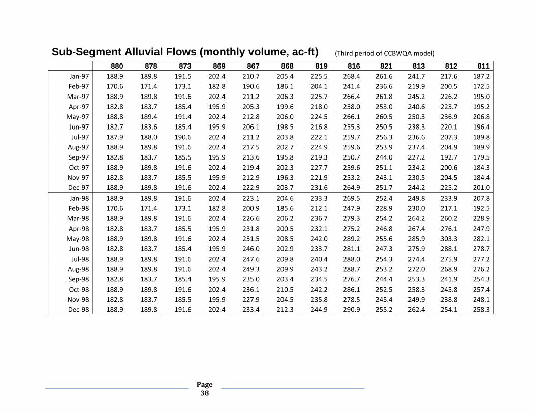
Page 38
Sub-Segment Alluvial Flows (monthly volume, ac-ft) (Third period of CCBWQA model)
880 878 873 869 867 868 819 816 821 813 812 811Jan‐97 188.9 189.8 191.5 202.4 210.7 205.4 225.5 268.4 261.6 241.7 217.6 187.2Feb‐97 170.6 171.4 173.1 182.8 190.6 186.1 204.1 241.4 236.6 219.9 200.5 172.5Mar‐97 188.9 189.8 191.6 202.4 211.2 206.3 225.7 266.4 261.8 245.2 226.2 195.0Apr‐97 182.8 183.7 185.4 195.9 205.3 199.6 218.0 258.0 253.0 240.6 225.7 195.2May‐97 188.8 189.4 191.4 202.4 212.8 206.0 224.5 266.1 260.5 250.3 236.9 206.8Jun‐97 182.7 183.6 185.4 195.9 206.1 198.5 216.8 255.3 250.5 238.3 220.1 196.4Jul‐97 187.9 188.0 190.6 202.4 211.2 203.8 222.1 259.7 256.3 236.6 207.3 189.8Aug‐97 188.9 189.8 191.6 202.4 217.5 202.7 224.9 259.6 253.9 237.4 204.9 189.9Sep‐97 182.8 183.7 185.5 195.9 213.6 195.8 219.3 250.7 244.0 227.2 192.7 179.5Oct‐97 188.9 189.8 191.6 202.4 219.4 202.3 227.7 259.6 251.1 234.2 200.6 184.3Nov‐97 182.8 183.7 185.5 195.9 212.9 196.3 221.9 253.2 243.1 230.5 204.5 184.4Dec‐97 188.9 189.8 191.6 202.4 222.9 203.7 231.6 264.9 251.7 244.2 225.2 201.0Jan‐98 188.9 189.8 191.6 202.4 223.1 204.6 233.3 269.5 252.4 249.8 233.9 207.8Feb‐98 170.6 171.4 173.1 182.8 200.9 185.6 212.1 247.9 228.9 230.0 217.1 192.5Mar‐98 188.9 189.8 191.6 202.4 226.6 206.2 236.7 279.3 254.2 264.2 260.2 228.9Apr‐98 182.8 183.7 185.5 195.9 231.8 200.5 232.1 275.2 246.8 267.4 276.1 247.9May‐98 188.9 189.8 191.6 202.4 251.5 208.5 242.0 289.2 255.6 285.9 303.3 282.1Jun‐98 182.8 183.7 185.4 195.9 246.0 202.9 233.7 281.1 247.3 275.9 288.1 278.7Jul‐98 188.9 189.8 191.6 202.4 247.6 209.8 240.4 288.0 254.3 274.4 275.9 277.2Aug‐98 188.9 189.8 191.6 202.4 249.3 209.9 243.2 288.7 253.2 272.0 268.9 276.2Sep‐98 182.8 183.7 185.4 195.9 235.0 203.4 234.5 276.7 244.4 253.3 241.9 254.3Oct‐98 188.9 189.8 191.6 202.4 236.1 210.5 242.2 286.1 252.5 258.3 245.8 257.4Nov‐98 182.8 183.7 185.5 195.9 227.9 204.5 235.8 278.5 245.4 249.9 238.8 248.1Dec‐98 188.9 189.8 191.6 202.4 233.4 212.3 244.9 290.9 255.2 262.4 254.1 258.3

Page 39
Sub-Segment Alluvial Flows (monthly volume, ac-ft) (Third period of CCBWQA model)
880 878 873 869 867 868 819 816 821 813 812 811Jan‐99 188.9 189.8 191.6 202.4 232.5 213.3 246.7 295.7 257.0 269.7 263.7 262.2Feb‐99 170.6 171.4 173.1 182.8 208.9 193.4 224.1 271.3 233.8 250.6 249.9 243.7Mar‐99 188.9 189.8 191.6 202.4 229.0 214.7 249.2 304.1 260.5 281.7 285.7 275.5Apr‐99 182.8 183.7 185.5 195.9 224.1 208.2 243.0 297.1 253.6 277.7 285.7 276.8May‐99 188.9 189.8 191.6 202.4 243.0 215.8 257.0 313.0 263.5 301.4 304.7 301.8Jun‐99 182.8 183.7 185.5 195.9 243.8 209.1 250.9 304.1 255.5 290.0 288.6 291.7Jul‐99 188.9 189.8 191.6 202.4 257.7 215.9 258.5 313.5 263.4 289.2 280.7 291.5Aug‐99 188.9 189.8 191.6 202.4 256.7 215.9 258.7 312.6 262.8 281.6 266.9 282.2Sep‐99 182.8 183.7 185.5 195.9 240.8 208.9 249.2 300.8 254.1 263.5 243.4 260.2Oct‐99 188.9 189.8 191.6 202.4 241.9 216.1 256.9 312.6 263.2 274.4 257.1 267.1Nov‐99 182.8 183.7 185.5 195.9 231.7 209.8 249.2 306.9 256.6 273.9 269.3 270.6Dec‐99 188.9 189.8 191.6 202.4 244.0 217.0 258.7 320.7 267.7 292.0 299.8 298.7Jan‐00 188.9 189.8 191.6 202.4 248.6 217.0 259.4 321.0 270.1 299.8 304.8 301.9Feb‐00 176.7 177.6 179.3 189.3 236.2 203.0 243.4 300.3 253.4 284.3 285.1 282.4Mar‐00 188.9 189.8 191.6 202.4 256.5 217.0 261.1 321.0 270.8 303.9 304.8 301.9Apr‐00 182.8 183.7 185.5 195.9 250.2 210.0 254.0 310.6 262.1 293.9 294.8 292.0May‐00 188.9 189.8 191.6 202.4 258.4 217.0 263.2 321.0 270.8 303.1 303.4 301.4Jun‐00 182.8 183.7 185.2 195.9 242.7 209.9 252.8 309.0 261.9 288.3 286.4 287.2Jul‐00 188.9 189.8 191.6 202.4 241.6 216.1 257.7 317.8 269.8 294.2 292.8 295.0Aug‐00 188.9 189.7 191.2 202.4 234.9 215.0 255.0 315.0 268.8 286.2 278.7 286.0Sep‐00 182.8 183.7 185.5 195.9 226.9 207.3 247.0 304.5 259.8 273.4 263.2 273.0Oct‐00 188.9 189.8 191.6 202.4 231.0 214.0 255.4 314.2 269.2 272.0 253.0 267.3Nov‐00 182.8 183.7 185.5 195.9 222.1 207.6 247.8 307.6 261.9 266.6 252.0 259.5Dec‐00 188.9 189.8 191.6 202.4 227.5 215.2 256.9 320.9 270.8 284.5 279.1 276.6

Page 40
Sub-Segment Alluvial Flows (monthly volume, ac-ft) (Third period of CCBWQA model)
880 878 873 869 867 868 819 816 821 813 812 811Jan‐01 188.9 189.8 191.6 202.4 225.8 215.7 257.6 321.0 270.8 293.3 300.4 297.6Feb‐01 170.6 171.4 173.1 182.8 205.5 195.3 233.5 289.9 244.6 271.9 275.3 272.7Mar‐01 188.9 189.8 191.6 202.4 231.0 216.6 259.2 321.0 270.8 303.9 304.8 301.9Apr‐01 182.8 183.7 185.5 195.9 226.0 209.9 252.0 310.6 262.1 294.1 294.9 292.2May‐01 188.9 189.8 191.6 202.4 242.0 217.0 262.0 320.9 270.8 302.6 302.5 301.2Jun‐01 182.8 183.7 185.3 195.9 232.6 209.7 252.3 307.3 261.9 278.8 266.4 275.1Jul‐01 188.8 189.5 191.2 202.4 232.5 215.5 257.0 311.8 269.6 271.1 243.2 260.0Aug‐01 188.8 189.2 191.2 202.4 227.3 214.1 254.0 307.9 268.4 260.1 224.3 242.1Sep‐01 182.8 182.9 185.0 195.9 215.3 206.0 242.9 294.5 259.0 243.9 204.6 219.7Oct‐01 188.9 189.8 191.5 202.4 218.2 212.1 248.2 301.5 267.5 248.0 207.4 217.5Nov‐01 182.8 183.7 185.5 195.9 210.2 205.2 240.6 292.6 260.0 242.4 209.0 210.4Dec‐01 188.9 189.8 191.6 202.4 218.8 212.2 250.0 305.8 270.2 256.9 228.5 221.9Jan‐02 188.9 189.8 191.6 202.4 219.1 212.5 251.0 308.6 270.8 261.7 237.1 225.5Feb‐02 170.6 171.4 173.1 182.8 198.7 192.2 227.6 281.0 244.6 242.2 223.7 208.7Mar‐02 188.9 189.8 191.6 202.4 222.4 213.0 253.1 314.4 270.8 276.0 262.0 240.6Apr‐02 182.8 183.7 185.4 195.9 214.7 206.2 245.3 304.4 262.1 268.6 255.6 235.8May‐02 188.9 189.7 191.5 202.4 219.3 212.7 251.6 309.5 270.8 264.8 237.4 226.5Jun‐02 182.8 183.7 185.4 195.9 212.1 205.1 242.3 296.1 261.8 247.6 212.5 206.3Jul‐02 188.9 189.6 191.4 202.4 218.0 210.4 248.8 302.8 269.3 246.7 202.1 198.8Aug‐02 188.8 188.5 190.5 202.4 214.0 208.6 245.1 298.3 267.7 237.6 186.2 183.1Sep‐02 182.8 183.7 185.5 195.9 207.8 200.5 236.6 286.9 258.1 228.8 179.3 172.1Oct‐02 188.9 189.8 191.6 202.4 215.2 206.4 244.9 296.1 266.5 233.6 181.3 171.0Nov‐02 149.5 150.3 151.7 160.2 170.0 163.3 194.2 233.6 211.5 180.9 137.2 127.9

Page 41
APPENDIX C . SUB-REACH SEDIMENT TRANSPORT CAPACITY AND SEDIMENT BALANCE
Sediment Transport Capacity by Sub-Reach (tons/month) 880 878 873 869 867 868 819 816 821 813 812
Inc. Length (ft) 2,180 1,715 5,270 1,032 2,615 696 2,353 5,657 2,903 1,378 627
Total Sed (tons) 1,114,398 1,014,397 970,610 806,145 870,066 615,726 597,878 547,001 388,284 363,510 700,714Total L (mi) 5.0 4.6 4.3 3.3 3.1 2.6 2.5 2.0 0.9 0.4 0.1
Jan‐95 0 0 0 0 0 0 0 0 0 0 0Feb‐95 252 364 168 448 420 84 0 0 0 0 0Mar‐95 961 1488 775 1519 1643 465 713 496 403 279 527Apr‐95 1320 1890 960 1890 2130 660 1050 810 690 600 1140May‐95 5704 8246 5332 6231 7161 3658 4433 4216 3100 3069 5828Jun‐95 41130 26670 37050 26610 28710 24870 26910 26970 18480 18180 36360Jul‐95 34689 24087 29481 21390 23095 20212 22227 22568 15593 15531 30814Aug‐95 13175 14136 11005 7626 7719 6696 5735 5425 3689 3844 7223Sep‐95 2820 4200 1860 3600 4350 1350 2610 2220 1890 1650 3300Oct‐95 8928 10788 6882 6603 7285 4278 5208 5115 3503 3658 6696Nov‐95 1890 3030 1560 3120 4020 1230 1680 1410 1170 960 2100Dec‐95 1240 2015 1054 2108 2418 744 806 341 310 248 372Jan‐96 496 806 434 1023 1116 310 124 62 62 31 124Feb‐96 319 522 261 667 667 174 0 0 0 0 0Mar‐96 496 806 403 930 992 279 186 0 0 0 0Apr‐96 1530 2400 1200 2490 3000 930 1440 600 540 390 780May‐96 403 465 155 465 496 155 310 186 186 155 341Jun‐96 4200 5910 2910 5340 6450 1980 3600 3390 2610 2370 4650Jul‐96 3131 4836 2418 4743 5704 1736 3069 2759 2294 1953 3937Aug‐96 868 1302 465 1054 1116 341 775 589 527 434 806Sep‐96 2640 3960 1560 2940 3480 1110 2430 2040 1770 1500 3000Oct‐96 3658 5239 2325 4433 5518 1798 3937 3813 2945 2883 5642Nov‐96 750 1050 420 900 930 270 780 660 540 450 870Dec‐96 248 0 0 186 62 0 0 0 0 0 0

Page 42
Sediment Transport Capacity by Sub-Reach (tons/month) 880 878 873 869 867 868 819 816 821 813 812
Jan‐97 217 62 0 186 93 0 0 0 0 0 0Feb‐97 280 448 84 336 252 56 0 0 0 0 0Mar‐97 279 465 248 620 620 155 0 0 0 0 0Apr‐97 930 1410 660 1350 1470 450 840 570 480 360 660May‐97 2325 3720 1953 3596 4309 1364 2790 2325 1984 1674 3348Jun‐97 1890 2910 1380 2670 3060 900 1440 1230 990 810 1560Jul‐97 7409 9362 5642 6386 7223 3813 4495 4464 3162 3131 5983Aug‐97 10726 12276 8215 7068 7595 6758 7750 8494 6076 6820 13733Sep‐97 63000 42180 56730 40500 43440 36930 35850 35010 23520 22140 43260Oct‐97 3441 5084 2573 4867 5921 1860 3317 2635 2232 1860 3627Nov‐97 4410 6360 3480 5490 6630 2100 3390 2550 2100 1680 3240Dec‐97 5425 7657 4619 6045 7037 2821 3782 3100 2449 2015 3875Jan‐98 5425 7781 4774 6076 7037 2883 3720 2573 2077 1581 2883Feb‐98 2520 4144 2212 4508 5376 1652 2100 532 420 140 140Mar‐98 4836 7130 4247 6014 7006 2790 3317 1798 1457 961 1519Apr‐98 27930 21510 25080 15870 15420 13080 10530 8490 5610 5070 8340May‐98 61876 41943 58714 36642 37014 31279 26598 24924 16461 15314 28551Jun‐98 13860 14310 11610 8280 8100 6930 5100 4200 3000 2640 4890Jul‐98 2139 3131 1426 2666 3038 930 1271 930 744 589 1116Aug‐98 82491 56668 75144 55986 61628 53103 47740 46872 32240 31403 62341Sep‐98 23190 19290 20100 14250 14550 12390 10800 10110 6720 6480 11820Oct‐98 1426 1829 558 1147 1271 372 465 279 248 217 434Nov‐98 5370 7350 4290 5820 6810 2790 3450 2400 1980 1620 2940Dec‐98 6913 9269 6200 6417 7223 3751 4154 3596 2728 2356 4650

Page 43
Sediment Transport Capacity by Sub-Reach (tons/month) 880 878 873 869 867 868 819 816 821 813 812
Jan‐99 10199 12369 9114 7099 7533 5797 4650 3565 2697 2170 3999Feb‐99 4788 6888 4200 5516 6384 2744 3136 1680 1372 784 1260Mar‐99 5921 8277 5239 6324 7192 3596 3720 2356 1922 1209 1767Apr‐99 2040 3240 1650 3300 3870 1170 1410 390 300 180 240May‐99 79298 55273 77686 53506 58156 50809 49662 48546 34162 32829 64883Jun‐99 115650 87690 115200 74610 79920 69090 56280 55080 38040 35580 73590Jul‐99 38068 25730 32674 21390 21080 18042 14880 13175 8835 8339 14725Aug‐99 14384 14105 9703 7254 7626 6603 5735 4867 3379 3379 6200Sep‐99 18420 16770 15270 11190 11460 9870 8490 7590 5130 4980 9000Oct‐99 3224 4774 2201 4123 4743 1426 1860 1178 961 713 1240Nov‐99 6870 8910 5520 6210 7020 3750 3780 2460 2040 1320 2160Dec‐99 9827 12028 8463 6975 7471 5301 4526 3441 2635 1953 3007Jan‐00 12245 13733 10850 8432 8060 7161 5084 4836 3317 2976 5270Feb‐00 10933 12499 9570 7221 7076 5916 4408 4437 3074 2784 5481Mar‐00 10819 12772 9455 7471 7564 6324 4743 4805 3410 3472 6758Apr‐00 32340 23280 28680 19770 19410 16950 12270 12300 8430 8580 16290May‐00 17639 16709 15531 11160 11067 9827 8184 8060 5611 5487 10633Jun‐00 16590 15930 14430 10710 11130 9840 7770 7170 5010 4830 8790Jul‐00 1798 2449 868 1705 1860 558 1054 775 651 496 961Aug‐00 6758 8153 4216 5952 7006 2790 4030 3782 2852 2666 5146Sep‐00 21810 18120 16590 12030 12330 10500 11700 11280 7530 7350 13590Oct‐00 14198 14353 10509 7595 7595 6386 5921 5146 3441 3441 6448Nov‐00 2670 4230 2100 4110 4830 1470 1860 480 390 300 480Dec‐00 4588 6851 4185 5983 7037 2914 3472 1953 1767 1178 2077

Page 44
Sediment Transport Capacity by Sub-Reach (tons/month) 880 878 873 869 867 868 819 816 821 813 812
Jan‐01 4712 6944 4154 6045 7068 3100 3596 3007 2604 1953 3038Feb‐01 8456 10584 7532 6300 6776 4956 4004 3892 2884 2548 4564Mar‐01 7440 9796 6510 6603 7285 4154 3937 3658 2883 2387 4774Apr‐01 9510 11640 8070 6780 7230 5220 4260 4110 3030 2940 5820May‐01 24490 20243 21638 14880 14942 12710 10819 11129 7657 7843 15655Jun‐01 35970 24660 31710 21930 22380 19080 15150 14760 10020 9990 19440Jul‐01 3193 4619 2139 4061 4774 1457 2356 1922 1612 1302 2542Aug‐01 3968 5022 2139 4185 5332 1767 3813 3689 2914 2914 5797Sep‐01 3690 5070 2370 4590 5460 1680 2550 2070 1740 1470 2820Oct‐01 4929 6076 2635 5053 5983 1798 3193 2728 2201 1829 3565Nov‐01 840 1170 300 690 690 210 120 0 0 0 0Dec‐01 6417 8804 5704 6355 7192 3596 4061 3131 2480 2015 3844Jan‐02 2604 4309 2325 4588 5394 1643 2170 806 682 465 806Feb‐02 2492 4116 2240 4228 4872 1484 2380 1400 1316 952 1792Mar‐02 3999 6231 3627 5766 6913 2449 3255 1984 1829 1271 2263Apr‐02 6330 8580 5430 6060 6900 3300 4050 3300 2670 2280 4290May‐02 837 1147 434 961 1054 310 248 62 186 31 62Jun‐02 2700 4140 2010 3750 4410 1350 2220 1830 1590 1320 2550Jul‐02 15190 14973 11377 8494 8618 7254 7440 6851 4495 4495 8184Aug‐02 6231 7874 4061 5921 7006 2759 4216 4030 2945 2790 5456Sep‐02 12120 12570 7620 6690 7230 5250 5760 5850 3900 4020 7410Oct‐02 14570 14663 11191 7936 7967 6851 6138 5518 3720 3813 7037Nov‐02 2640 4170 2160 4080 4860 1500 2130 1170 990 840 1590Dec‐02 837 1364 713 1457 1705 527 465 0 0 0 0

Page 45
Sediment Load Difference by Sub‐Reach (tons/month)878 873 869 867 868 819 816 821 813 812
Inc. Length (ft) 2,180 1,715 5,270 1,032 2,615 696 2,353 5,657 2,903 1,378Total Sed (tons) 100,001 43,787 164,465 ‐63,921 254,340 17,848 50,877 158,717 24,774 ‐337,204
Total L (mi) 5.0 4.6 4.3 3.3 3.1 2.6 2.5 2.0 0.9 0.4Jan‐95 0 0 0 0 0 0 0 0 0 0Feb‐95 ‐112 196 ‐280 28 336 84 0 0 0 0Mar‐95 ‐527 713 ‐744 ‐124 1178 ‐248 217 93 124 ‐248Apr‐95 ‐570 930 ‐930 ‐240 1470 ‐390 240 120 90 ‐540May‐95 ‐2542 2914 ‐899 ‐930 3503 ‐775 217 1116 31 ‐2759Jun‐95 14460 ‐10380 10440 ‐2100 3840 ‐2040 ‐60 8490 300 ‐18180Jul‐95 10602 ‐5394 8091 ‐1705 2883 ‐2015 ‐341 6975 62 ‐15283Aug‐95 ‐961 3131 3379 ‐93 1023 961 310 1736 ‐155 ‐3379Sep‐95 ‐1380 2340 ‐1740 ‐750 3000 ‐1260 390 330 240 ‐1650Oct‐95 ‐1860 3906 279 ‐682 3007 ‐930 93 1612 ‐155 ‐3038Nov‐95 ‐1140 1470 ‐1560 ‐900 2790 ‐450 270 240 210 ‐1140Dec‐95 ‐775 961 ‐1054 ‐310 1674 ‐62 465 31 62 ‐124Jan‐96 ‐310 372 ‐589 ‐93 806 186 62 0 31 ‐93Feb‐96 ‐203 261 ‐406 0 493 174 0 0 0 0Mar‐96 ‐310 403 ‐527 ‐62 713 93 186 0 0 0Apr‐96 ‐870 1200 ‐1290 ‐510 2070 ‐510 840 60 150 ‐390May‐96 ‐62 310 ‐310 ‐31 341 ‐155 124 0 31 ‐186Jun‐96 ‐1710 3000 ‐2430 ‐1110 4470 ‐1620 210 780 240 ‐2280Jul‐96 ‐1705 2418 ‐2325 ‐961 3968 ‐1333 310 465 341 ‐1984Aug‐96 ‐434 837 ‐589 ‐62 775 ‐434 186 62 93 ‐372Sep‐96 ‐1320 2400 ‐1380 ‐540 2370 ‐1320 390 270 270 ‐1500Oct‐96 ‐1581 2914 ‐2108 ‐1085 3720 ‐2139 124 868 62 ‐2759Nov‐96 ‐300 630 ‐480 ‐30 660 ‐510 120 120 90 ‐420Dec‐96 248 0 ‐186 124 62 0 0 0 0 0

Page 46
Sediment Load Difference by Sub‐Reach (tons/month)878 873 869 867 868 819 816 821 813 812
Jan‐97 155 62 ‐186 93 93 0 0 0 0 0Feb‐97 ‐168 364 ‐252 84 196 56 0 0 0 0Mar‐97 ‐186 217 ‐372 0 465 155 0 0 0 0Apr‐97 ‐480 750 ‐690 ‐120 1020 ‐390 270 90 120 ‐300May‐97 ‐1395 1767 ‐1643 ‐713 2945 ‐1426 465 341 310 ‐1674Jun‐97 ‐1020 1530 ‐1290 ‐390 2160 ‐540 210 240 180 ‐750Jul‐97 ‐1953 3720 ‐744 ‐837 3410 ‐682 31 1302 31 ‐2852Aug‐97 ‐1550 4061 1147 ‐527 837 ‐992 ‐744 2418 ‐744 ‐6913Sep‐97 20820 ‐14550 16230 ‐2940 6510 1080 840 11490 1380 ‐21120Oct‐97 ‐1643 2511 ‐2294 ‐1054 4061 ‐1457 682 403 372 ‐1767Nov‐97 ‐1950 2880 ‐2010 ‐1140 4530 ‐1290 840 450 420 ‐1560Dec‐97 ‐2232 3038 ‐1426 ‐992 4216 ‐961 682 651 434 ‐1860Jan‐98 ‐2356 3007 ‐1302 ‐961 4154 ‐837 1147 496 496 ‐1302Feb‐98 ‐1624 1932 ‐2296 ‐868 3724 ‐448 1568 112 280 0Mar‐98 ‐2294 2883 ‐1767 ‐992 4216 ‐527 1519 341 496 ‐558Apr‐98 6420 ‐3570 9210 450 2340 2550 2040 2880 540 ‐3270May‐98 19933 ‐16771 22072 ‐372 5735 4681 1674 8463 1147 ‐13237Jun‐98 ‐450 2700 3330 180 1170 1830 900 1200 360 ‐2250Jul‐98 ‐992 1705 ‐1240 ‐372 2108 ‐341 341 186 155 ‐527Aug‐98 25823 ‐18476 19158 ‐5642 8525 5363 868 14632 837 ‐30938Sep‐98 3900 ‐810 5850 ‐300 2160 1590 690 3390 240 ‐5340Oct‐98 ‐403 1271 ‐589 ‐124 899 ‐93 186 31 31 ‐217Nov‐98 ‐1980 3060 ‐1530 ‐990 4020 ‐660 1050 420 360 ‐1320Dec‐98 ‐2356 3069 ‐217 ‐806 3472 ‐403 558 868 372 ‐2294

Page 47
Sediment Load Difference by Sub‐Reach (tons/month)878 873 869 867 868 819 816 821 813 812
Jan‐99 ‐2170 3255 2015 ‐434 1736 1147 1085 868 527 ‐1829Feb‐99 ‐2100 2688 ‐1316 ‐868 3640 ‐392 1456 308 588 ‐476Mar‐99 ‐2356 3038 ‐1085 ‐868 3596 ‐124 1364 434 713 ‐558Apr‐99 ‐1200 1590 ‐1650 ‐570 2700 ‐240 1020 90 120 ‐60May‐99 24025 ‐22413 24180 ‐4650 7347 1147 1116 14384 1333 ‐32054Jun‐99 27960 ‐27510 40590 ‐5310 10830 12810 1200 17040 2460 ‐38010Jul‐99 12338 ‐6944 11284 310 3038 3162 1705 4340 496 ‐6386Aug‐99 279 4402 2449 ‐372 1023 868 868 1488 0 ‐2821Sep‐99 1650 1500 4080 ‐270 1590 1380 900 2460 150 ‐4020Oct‐99 ‐1550 2573 ‐1922 ‐620 3317 ‐434 682 217 248 ‐527Nov‐99 ‐2040 3390 ‐690 ‐810 3270 ‐30 1320 420 720 ‐840Dec‐99 ‐2201 3565 1488 ‐496 2170 775 1085 806 682 ‐1054Jan‐00 ‐1488 2883 2418 372 899 2077 248 1519 341 ‐2294Feb‐00 ‐1566 2929 2349 145 1160 1508 ‐29 1363 290 ‐2697Mar‐00 ‐1953 3317 1984 ‐93 1240 1581 ‐62 1395 ‐62 ‐3286Apr‐00 9060 ‐5400 8910 360 2460 4680 ‐30 3870 ‐150 ‐7710May‐00 930 1178 4371 93 1240 1643 124 2449 124 ‐5146Jun‐00 660 1500 3720 ‐420 1290 2070 600 2160 180 ‐3960Jul‐00 ‐651 1581 ‐837 ‐155 1302 ‐496 279 124 155 ‐465Aug‐00 ‐1395 3937 ‐1736 ‐1054 4216 ‐1240 248 930 186 ‐2480Sep‐00 3690 1530 4560 ‐300 1830 ‐1200 420 3750 180 ‐6240Oct‐00 ‐155 3844 2914 0 1209 465 775 1705 0 ‐3007Nov‐00 ‐1560 2130 ‐2010 ‐720 3360 ‐390 1380 90 90 ‐180Dec‐00 ‐2263 2666 ‐1798 ‐1054 4123 ‐558 1519 186 589 ‐899

Page 48
Sediment Load Difference by Sub‐Reach (tons/month)878 873 869 867 868 819 816 821 813 812
Jan‐01 ‐2232 2790 ‐1891 ‐1023 3968 ‐496 589 403 651 ‐1085Feb‐01 ‐2128 3052 1232 ‐476 1820 952 112 1008 336 ‐2016Mar‐01 ‐2356 3286 ‐93 ‐682 3131 217 279 775 496 ‐2387Apr‐01 ‐2130 3570 1290 ‐450 2010 960 150 1080 90 ‐2880May‐01 4247 ‐1395 6758 ‐62 2232 1891 ‐310 3472 ‐186 ‐7812Jun‐01 11310 ‐7050 9780 ‐450 3300 3930 390 4740 30 ‐9450Jul‐01 ‐1426 2480 ‐1922 ‐713 3317 ‐899 434 310 310 ‐1240Aug‐01 ‐1054 2883 ‐2046 ‐1147 3565 ‐2046 124 775 0 ‐2883Sep‐01 ‐1380 2700 ‐2220 ‐870 3780 ‐870 480 330 270 ‐1350Oct‐01 ‐1147 3441 ‐2418 ‐930 4185 ‐1395 465 527 372 ‐1736Nov‐01 ‐330 870 ‐390 0 480 90 120 0 0 0Dec‐01 ‐2387 3100 ‐651 ‐837 3596 ‐465 930 651 465 ‐1829Jan‐02 ‐1705 1984 ‐2263 ‐806 3751 ‐527 1364 124 217 ‐341Feb‐02 ‐1624 1876 ‐1988 ‐644 3388 ‐896 980 84 364 ‐840Mar‐02 ‐2232 2604 ‐2139 ‐1147 4464 ‐806 1271 155 558 ‐992Apr‐02 ‐2250 3150 ‐630 ‐840 3600 ‐750 750 630 390 ‐2010May‐02 ‐310 713 ‐527 ‐93 744 62 186 ‐124 155 ‐31Jun‐02 ‐1440 2130 ‐1740 ‐660 3060 ‐870 390 240 270 ‐1230Jul‐02 217 3596 2883 ‐124 1364 ‐186 589 2356 0 ‐3689Aug‐02 ‐1643 3813 ‐1860 ‐1085 4247 ‐1457 186 1085 155 ‐2666Sep‐02 ‐450 4950 930 ‐540 1980 ‐510 ‐90 1950 ‐120 ‐3390Oct‐02 ‐93 3472 3255 ‐31 1116 713 620 1798 ‐93 ‐3224Nov‐02 ‐1530 2010 ‐1920 ‐780 3360 ‐630 960 180 150 ‐750Dec‐02 ‐527 651 ‐744 ‐248 1178 62 465 0 0 0
C h e r r y C r e e k S e d i m e n t a t i o n S t u d y R e s e r v o i r t o P i n e L a n e
S e d i m e n t B u d g e t
March 2011 Prepared for: Southeast Metropolitan Stormwater Authority 76 Inverness Drive Englewood, Colorado Submitted to: Ms. Molly Trujillo, P.E. Prepared by:
GK COTTON CONSULTING, INC 10290 S. Progress Way, #205 PO Box 1060 Parker, CO 80134-1060

C H E R RY C R E E K S E D I M E N TAT I O N S T U DY
SEDIMENT BUDGET
Table of Contents
Introduction............................................................................................................................. 3
Description of Water Operations ............................................................................................. 3
CCBWQA Model Structure ................................................................................................................ 4
Flow Pattern .................................................................................................................................... 4
Sub‐Reach Characteristics ........................................................................................................ 5
Sediment Transport Ratings .................................................................................................... 7
HEC‐RAS Results ............................................................................................................................... 7
Time Step Scaling ............................................................................................................................. 8
Sediment Budget ..................................................................................................................... 9
Supply Reach .................................................................................................................................... 9
Sediment Budget by Sub‐Reach ...................................................................................................... 12
Summary and Findings .......................................................................................................... 14
References ............................................................................................................................. 14
Appendix A. Sub‐Reach Cross Sections ................................................................................... 15
Appendix B. Sub‐Reach Hydraulic Design Data / Sediment Transport Rating ......................... 21
Appendix C. Sub‐Reach Flow Data from CCBWQA Model ....................................................... 33
Appendix C. Sub‐Reach Sediment Transport Capacity ............................................................ 41
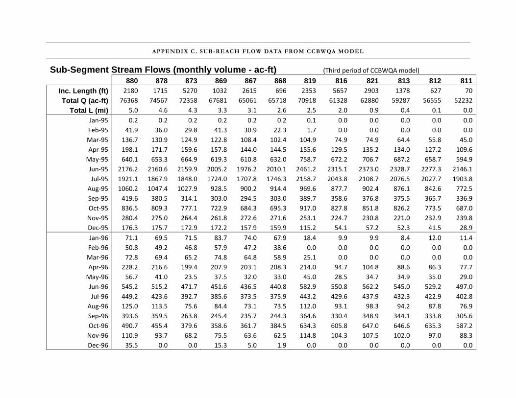
APPENDIX C . SUB-REACH FLOW DATA FROM CCBWQA MODEL
Sub-Segment Stream Flows (monthly volume - ac-ft) (Third period of CCBWQA model)
880 878 873 869 867 868 819 816 821 813 812 811Inc. Length (ft) 2180 1715 5270 1032 2615 696 2353 5657 2903 1378 627 70Total Q (ac-ft) 76368 74567 72358 67681 65061 65718 70918 61328 62880 59287 56555 52232
Total L (mi) 5.0 4.6 4.3 3.3 3.1 2.6 2.5 2.0 0.9 0.4 0.1 0.0Jan‐95 0.2 0.2 0.2 0.2 0.2 0.2 0.1 0.0 0.0 0.0 0.0 0.0Feb‐95 41.9 36.0 29.8 41.3 30.9 22.3 1.7 0.0 0.0 0.0 0.0 0.0Mar‐95 136.7 130.9 124.9 122.8 108.4 102.4 104.9 74.9 74.9 64.4 55.8 45.0Apr‐95 198.1 171.7 159.6 157.8 144.0 144.5 155.6 129.5 135.2 134.0 127.2 109.6May‐95 640.1 653.3 664.9 619.3 610.8 632.0 758.7 672.2 706.7 687.2 658.7 594.9Jun‐95 2176.2 2160.6 2159.9 2005.2 1976.2 2010.1 2461.2 2315.1 2373.0 2328.7 2277.3 2146.1Jul‐95 1921.1 1867.9 1848.0 1724.0 1707.8 1746.3 2158.7 2043.8 2108.7 2076.5 2027.7 1903.8Aug‐95 1060.2 1047.4 1027.9 928.5 900.2 914.4 969.6 877.7 902.4 876.1 842.6 772.5Sep‐95 419.6 380.5 314.1 303.0 294.5 303.0 389.7 358.6 376.8 375.5 365.7 336.9Oct‐95 836.5 809.3 777.1 722.9 684.3 695.3 917.0 827.8 851.8 826.2 773.5 687.0Nov‐95 280.4 275.0 264.4 261.8 272.6 271.6 253.1 224.7 230.8 221.0 232.9 239.8Dec‐95 176.3 175.7 172.9 172.2 157.9 159.9 115.2 54.1 57.2 52.3 41.5 28.9Jan‐96 71.1 69.5 71.5 83.7 74.0 67.9 18.4 9.9 9.9 8.4 12.0 11.4Feb‐96 50.8 49.2 46.8 57.9 47.2 38.6 0.0 0.0 0.0 0.0 0.0 0.0Mar‐96 72.8 69.4 65.2 74.8 64.8 58.9 25.1 0.0 0.0 0.0 0.0 0.0Apr‐96 228.2 216.6 199.4 207.9 203.1 208.3 214.0 94.7 104.8 88.6 86.3 77.7May‐96 56.7 41.0 23.5 37.5 32.0 33.0 45.0 28.5 34.7 34.9 35.0 29.0Jun‐96 545.2 515.2 471.7 451.6 436.5 440.8 582.9 550.8 562.2 545.0 529.2 497.0Jul‐96 449.2 423.6 392.7 385.6 373.5 375.9 443.2 429.6 437.9 432.3 422.9 402.8Aug‐96 125.0 113.5 75.6 84.4 73.1 73.5 112.0 93.1 98.3 94.2 87.8 76.9Sep‐96 393.6 359.5 263.8 245.4 235.7 244.3 364.6 330.4 348.9 344.1 333.8 305.6Oct‐96 490.7 455.4 379.6 358.6 361.7 384.5 634.3 605.8 647.0 646.6 635.3 587.2Nov‐96 110.9 93.7 68.2 75.5 63.6 62.5 114.8 104.3 107.5 102.0 97.0 88.3Dec‐96 35.5 0.0 0.0 15.3 5.0 1.9 0.0 0.0 0.0 0.0 0.0 0.0

Page 34
Sub-Segment Stream Flows (monthly volume - ac-ft) (Third period of CCBWQA model)
880 878 873 869 867 868 819 816 821 813 812 811Jan‐97 32.4 4.3 0.0 15.9 5.1 1.9 0.0 0.0 0.0 0.0 0.0 0.0Feb‐97 45.7 44.5 16.3 30.0 19.2 13.7 0.0 0.0 0.0 0.0 0.0 0.0Mar‐97 40.9 40.8 39.1 49.7 40.0 31.9 0.0 0.0 0.0 0.0 0.0 0.0Apr‐97 136.7 127.7 109.3 112.1 98.7 96.9 127.0 92.4 94.4 81.8 72.5 59.0May‐97 336.9 326.8 316.6 292.6 282.6 293.0 405.9 361.8 382.0 372.7 359.0 324.2Jun‐97 283.0 263.0 232.0 224.6 206.9 203.1 215.8 195.8 195.8 184.5 173.3 158.3Jul‐97 749.1 722.8 689.0 659.6 642.0 648.3 770.4 716.3 730.0 706.4 680.3 639.6Aug‐97 934.3 899.8 864.6 861.3 881.2 919.1 1158.7 1150.6 1213.7 1254.4 1262.0 1213.5Sep‐97 2860.5 2826.6 2781.6 2596.0 2532.2 2541.9 2909.0 2708.4 2724.9 2617.2 2526.7 2394.6Oct‐97 472.8 445.3 415.7 393.8 387.6 398.1 493.9 410.8 429.1 409.2 389.8 349.2Nov‐97 559.9 546.7 524.5 481.7 458.2 460.2 539.3 411.5 415.6 383.1 359.3 324.7Dec‐97 621.4 617.2 611.2 569.3 539.6 539.5 603.1 483.2 483.1 446.5 416.1 375.4Jan‐98 622.6 624.0 623.1 577.4 546.1 546.1 588.1 398.4 398.3 351.9 311.6 258.4Feb‐98 401.8 400.8 398.8 404.3 389.8 389.8 335.8 93.3 91.6 31.5 17.6 9.0Mar‐98 581.6 581.6 581.0 561.8 533.8 533.8 496.3 280.7 280.2 210.4 162.3 112.0Apr‐98 1715.7 1710.5 1711.6 1470.3 1374.7 1379.3 1415.9 1173.9 1181.2 1065.8 960.2 819.5May‐98 2767.9 2767.7 2784.6 2390.1 2249.4 2256.7 2396.7 2166.3 2177.8 2057.6 1938.0 1749.5Jun‐98 1115.8 1101.4 1082.1 993.9 944.1 950.9 924.4 694.6 704.7 607.8 557.6 416.7Jul‐98 308.2 275.1 230.7 216.9 199.5 197.8 184.6 142.5 144.6 132.7 119.5 99.6Aug‐98 3331.1 3267.3 3224.6 3113.0 3075.2 3097.8 3375.3 3166.4 3203.8 3158.8 3081.3 2958.7Sep‐98 1531.2 1520.5 1501.2 1377.6 1329.3 1337.0 1437.4 1299.7 1313.2 1237.9 1178.3 1073.2Oct‐98 203.6 158.9 88.8 92.5 82.7 82.2 66.9 43.1 47.2 47.5 46.2 39.6Nov‐98 629.2 612.6 595.1 563.4 539.5 544.0 553.3 385.4 392.5 371.3 328.1 285.2Dec‐98 717.4 717.2 729.3 668.2 640.2 641.9 690.9 566.7 571.8 526.4 509.7 466.8

Page 35
Sub-Segment Stream Flows (monthly volumes - ac-ft) (Third period of CCBWQA model)
880 878 873 869 867 868 819 816 821 813 812 811Jan‐99 905.9 907.3 918.5 869.3 837.2 837.2 806.9 564.4 563.2 480.3 429.9 390.8Feb‐99 613.5 614.2 613.3 589.5 564.7 564.7 533.4 289.9 289.5 193.1 150.2 114.0Mar‐99 654.7 655.3 657.5 644.1 625.1 625.1 585.9 366.4 366.4 269.1 189.8 118.7Apr‐99 302.0 293.9 277.4 276.1 261.3 260.6 211.1 61.9 61.4 38.2 28.2 19.6May‐99 3247.3 3222.6 3288.5 3026.3 2967.9 3016.6 3453.7 3233.9 3311.6 3244.4 3155.8 2952.3Jun‐99 4229.0 4233.6 4238.5 3799.4 3679.2 3698.8 3788.0 3558.3 3589.7 3468.4 3470.1 3429.8Jul‐99 2033.8 2004.5 1965.5 1725.1 1619.1 1633.6 1703.0 1489.7 1512.5 1416.6 1314.9 1140.8Aug‐99 1118.7 1044.4 953.4 900.5 893.8 906.1 969.7 780.7 801.9 760.9 705.7 643.4Sep‐99 1328.3 1305.7 1274.7 1190.5 1155.0 1169.0 1248.2 1099.2 1121.1 1054.0 1004.8 906.5Oct‐99 455.8 418.0 359.2 334.6 309.6 308.9 270.8 182.1 185.1 159.9 134.8 100.9Nov‐99 730.2 714.2 693.0 672.7 652.4 655.2 631.9 397.7 401.9 303.0 239.1 192.5Dec‐99 886.3 883.8 879.1 839.3 785.6 793.3 775.5 539.3 539.3 430.9 323.1 165.0Jan‐00 1013.4 1014.9 1020.5 986.1 923.9 950.5 904.3 779.0 779.0 667.4 587.8 498.6Feb‐00 985.8 985.7 985.4 934.1 852.5 882.7 827.7 764.6 776.0 668.8 662.2 663.6Mar‐00 938.8 939.2 939.2 915.8 852.0 883.6 831.1 772.3 817.6 782.4 779.7 780.7Apr‐00 1877.2 1864.8 1853.7 1677.2 1572.9 1606.5 1549.0 1458.1 1498.6 1472.1 1423.0 1397.9May‐00 1267.6 1255.8 1262.1 1166.1 1111.4 1145.1 1195.8 1115.6 1155.8 1097.8 1086.8 1060.7Jun‐00 1246.3 1236.8 1232.3 1161.2 1135.6 1167.7 1184.9 1063.0 1102.6 1034.3 991.0 917.2Jul‐00 258.0 213.2 141.9 139.0 122.1 120.3 152.4 122.8 122.8 112.2 101.9 87.4Aug‐00 709.3 648.7 577.6 547.0 529.6 536.2 657.5 600.4 613.6 594.4 572.3 529.8Sep‐00 1474.0 1420.2 1338.9 1243.9 1205.5 1213.8 1506.3 1387.4 1402.5 1338.6 1278.5 1189.9Oct‐00 1110.7 1064.4 1000.3 926.1 888.5 888.5 989.3 829.0 828.9 779.1 737.7 677.9Nov‐00 398.2 381.4 354.4 343.2 326.1 326.1 276.7 78.7 78.3 66.0 52.6 40.5Dec‐00 562.8 564.8 575.9 558.0 542.0 547.8 527.9 302.8 339.4 261.6 224.5 197.8

Page 36
Sub-Segment Stream Flows (monthly volumes - ac-ft) (Third period of CCBWQA model)
880 878 873 869 867 868 819 816 821 813 812 811Jan‐01 572.0 570.4 572.6 572.9 563.4 569.7 557.5 468.3 527.9 430.5 327.0 181.6Feb‐01 860.9 864.8 872.5 838.5 809.5 810.1 755.0 690.7 740.6 632.6 558.7 452.2Mar‐01 749.6 750.3 751.8 724.2 684.0 684.0 634.8 576.9 621.1 529.4 524.6 526.0Apr‐01 886.0 882.2 872.5 840.7 802.0 802.0 744.6 677.7 716.5 684.7 682.6 682.7May‐01 1551.7 1545.2 1537.7 1386.7 1324.3 1330.8 1410.5 1348.8 1388.2 1363.8 1363.1 1361.5Jun‐01 2004.6 1983.5 1968.4 1786.0 1708.4 1722.1 1754.3 1624.4 1657.6 1614.9 1577.5 1517.5Jul‐01 454.0 403.3 346.9 330.2 313.3 313.5 340.8 300.7 305.8 288.9 272.7 248.3Aug‐01 515.4 440.4 345.8 338.3 348.8 378.1 607.4 585.1 636.1 652.8 653.0 610.6Sep‐01 502.8 456.6 399.2 384.7 368.5 372.3 383.5 334.2 344.3 332.8 314.6 284.4Oct‐01 586.8 513.9 425.9 410.5 390.5 387.9 472.5 423.2 423.2 402.1 382.7 357.2Nov‐01 126.6 105.6 48.3 58.3 47.4 43.6 16.1 0.0 0.0 0.0 0.0 0.0Dec‐01 687.2 688.7 694.2 652.5 625.0 626.3 663.9 491.4 493.5 448.3 414.8 376.1Jan‐02 376.4 378.2 379.1 371.5 353.2 353.2 315.5 126.3 130.9 100.4 85.2 68.1Feb‐02 396.4 399.2 400.5 379.5 353.3 355.1 382.5 240.0 281.6 231.6 211.9 181.9Mar‐02 518.5 522.8 527.8 505.5 492.3 493.4 482.5 310.4 347.4 282.6 243.6 212.3Apr‐02 695.7 692.3 686.2 625.5 597.3 606.3 697.9 538.7 584.1 522.4 481.7 420.3May‐02 119.5 100.9 71.9 78.8 68.0 64.4 33.9 10.5 35.2 8.2 5.7 2.5Jun‐02 402.1 375.1 336.8 314.9 298.4 301.9 332.1 295.8 314.9 298.6 284.3 257.0Jul‐02 1157.2 1114.3 1048.2 990.6 959.3 959.3 1132.7 1013.8 1017.4 971.4 931.7 876.4Aug‐02 675.1 630.3 564.8 545.1 528.3 530.9 700.7 642.3 650.5 628.7 608.6 572.6Sep‐02 1027.3 956.9 841.5 817.2 801.1 805.4 992.5 943.1 953.9 922.2 897.4 855.5Oct‐02 1128.0 1089.7 1038.2 949.2 916.7 926.3 1011.6 895.2 910.0 863.8 819.0 748.2Nov‐02 391.1 378.2 360.4 343.0 328.8 335.4 317.7 185.8 195.8 189.1 178.1 154.9Dec‐02 118.9 118.4 113.5 119.2 110.8 110.8 68.2 0.0 0.0 0.0 0.0 0.0

Page 37
Sub-Segment Alluvial Flows (monthly volume, ac-ft) (Third period of CCBWQA model)
880 878 873 869 867 868 819 816 821 813 812 811Jan‐95 0.3 0.3 0.3 0.3 0.3 0.3 0.3 0.4 0.4 0.3 0.2 0.2Feb‐95 184.8 185.7 187.5 198.0 209.5 202.3 239.8 287.0 262.5 221.8 168.6 152.5Mar‐95 170.6 171.4 173.1 182.8 193.5 187.4 220.4 264.2 243.2 208.5 165.4 143.7Apr‐95 188.9 189.8 191.6 202.4 214.8 207.8 243.0 292.2 270.1 235.4 194.2 164.3May‐95 182.8 183.7 185.5 195.9 209.5 201.2 234.4 282.9 261.8 233.4 200.4 167.0Jun‐95 188.9 189.8 191.6 202.4 219.9 208.1 242.7 294.2 270.8 249.4 223.4 186.3Jul‐95 182.8 183.7 185.5 195.9 221.6 201.4 236.7 286.0 261.7 246.0 222.7 191.1Aug‐95 188.9 189.8 191.6 202.4 232.7 207.8 245.4 294.4 269.2 251.2 221.7 195.7Sep‐95 188.9 189.8 191.3 202.4 228.9 207.3 242.8 290.5 267.6 242.6 204.9 184.3Oct‐95 182.8 183.7 185.4 195.9 219.2 200.3 233.2 278.5 257.8 230.3 190.1 171.4Nov‐95 188.9 189.8 191.6 202.4 226.3 207.4 241.7 287.2 266.3 238.8 198.7 177.3Dec‐95 182.8 183.7 185.5 195.9 216.7 201.6 234.6 277.4 258.4 232.9 198.4 173.7Jan‐96 188.9 189.8 191.6 202.4 222.5 209.1 243.6 286.6 267.9 243.8 213.1 184.2Feb‐96 188.9 189.8 191.6 202.4 220.7 210.1 244.2 284.5 268.7 242.2 210.8 182.6Mar‐96 176.7 177.6 179.3 189.3 205.0 197.3 228.5 264.8 252.0 226.9 198.8 171.4Apr‐96 188.9 189.8 191.6 202.4 217.7 211.2 244.0 283.5 269.7 245.4 218.5 187.3May‐96 182.8 183.6 185.4 195.9 209.1 204.3 235.5 275.6 261.0 240.7 216.1 184.7Jun‐96 188.7 189.1 191.2 202.4 214.1 210.5 241.0 282.5 269.2 245.9 217.9 188.2Jul‐96 182.7 183.5 185.3 195.9 207.1 202.8 231.8 272.5 259.3 240.7 216.3 186.8Aug‐96 187.9 187.9 190.7 202.4 212.0 208.1 236.7 279.9 265.9 248.8 224.9 194.6Sep‐96 187.5 186.3 190.4 202.4 210.1 206.4 233.7 275.8 263.6 239.5 206.1 182.5Oct‐96 181.6 179.4 184.7 195.9 202.8 198.5 223.9 264.6 253.3 228.8 194.2 172.0Nov‐96 188.8 185.4 191.1 202.4 209.8 204.6 229.6 272.1 260.9 237.5 204.1 179.3Dec‐96 182.8 181.0 185.0 195.9 203.3 198.0 220.6 261.9 252.5 230.2 199.9 174.1Jan‐95 188.9 189.2 191.0 202.4 210.4 205.0 226.6 269.5 261.3 239.8 212.3 183.4

Page 38
Sub-Segment Alluvial Flows (monthly volume, ac-ft) (Third period of CCBWQA model)
880 878 873 869 867 868 819 816 821 813 812 811Jan‐97 188.9 189.8 191.5 202.4 210.7 205.4 225.5 268.4 261.6 241.7 217.6 187.2Feb‐97 170.6 171.4 173.1 182.8 190.6 186.1 204.1 241.4 236.6 219.9 200.5 172.5Mar‐97 188.9 189.8 191.6 202.4 211.2 206.3 225.7 266.4 261.8 245.2 226.2 195.0Apr‐97 182.8 183.7 185.4 195.9 205.3 199.6 218.0 258.0 253.0 240.6 225.7 195.2May‐97 188.8 189.4 191.4 202.4 212.8 206.0 224.5 266.1 260.5 250.3 236.9 206.8Jun‐97 182.7 183.6 185.4 195.9 206.1 198.5 216.8 255.3 250.5 238.3 220.1 196.4Jul‐97 187.9 188.0 190.6 202.4 211.2 203.8 222.1 259.7 256.3 236.6 207.3 189.8Aug‐97 188.9 189.8 191.6 202.4 217.5 202.7 224.9 259.6 253.9 237.4 204.9 189.9Sep‐97 182.8 183.7 185.5 195.9 213.6 195.8 219.3 250.7 244.0 227.2 192.7 179.5Oct‐97 188.9 189.8 191.6 202.4 219.4 202.3 227.7 259.6 251.1 234.2 200.6 184.3Nov‐97 182.8 183.7 185.5 195.9 212.9 196.3 221.9 253.2 243.1 230.5 204.5 184.4Dec‐97 188.9 189.8 191.6 202.4 222.9 203.7 231.6 264.9 251.7 244.2 225.2 201.0Jan‐98 188.9 189.8 191.6 202.4 223.1 204.6 233.3 269.5 252.4 249.8 233.9 207.8Feb‐98 170.6 171.4 173.1 182.8 200.9 185.6 212.1 247.9 228.9 230.0 217.1 192.5Mar‐98 188.9 189.8 191.6 202.4 226.6 206.2 236.7 279.3 254.2 264.2 260.2 228.9Apr‐98 182.8 183.7 185.5 195.9 231.8 200.5 232.1 275.2 246.8 267.4 276.1 247.9May‐98 188.9 189.8 191.6 202.4 251.5 208.5 242.0 289.2 255.6 285.9 303.3 282.1Jun‐98 182.8 183.7 185.4 195.9 246.0 202.9 233.7 281.1 247.3 275.9 288.1 278.7Jul‐98 188.9 189.8 191.6 202.4 247.6 209.8 240.4 288.0 254.3 274.4 275.9 277.2Aug‐98 188.9 189.8 191.6 202.4 249.3 209.9 243.2 288.7 253.2 272.0 268.9 276.2Sep‐98 182.8 183.7 185.4 195.9 235.0 203.4 234.5 276.7 244.4 253.3 241.9 254.3Oct‐98 188.9 189.8 191.6 202.4 236.1 210.5 242.2 286.1 252.5 258.3 245.8 257.4Nov‐98 182.8 183.7 185.5 195.9 227.9 204.5 235.8 278.5 245.4 249.9 238.8 248.1Dec‐98 188.9 189.8 191.6 202.4 233.4 212.3 244.9 290.9 255.2 262.4 254.1 258.3

Page 39
Sub-Segment Alluvial Flows (monthly volume, ac-ft) (Third period of CCBWQA model)
880 878 873 869 867 868 819 816 821 813 812 811Jan‐99 188.9 189.8 191.6 202.4 232.5 213.3 246.7 295.7 257.0 269.7 263.7 262.2Feb‐99 170.6 171.4 173.1 182.8 208.9 193.4 224.1 271.3 233.8 250.6 249.9 243.7Mar‐99 188.9 189.8 191.6 202.4 229.0 214.7 249.2 304.1 260.5 281.7 285.7 275.5Apr‐99 182.8 183.7 185.5 195.9 224.1 208.2 243.0 297.1 253.6 277.7 285.7 276.8May‐99 188.9 189.8 191.6 202.4 243.0 215.8 257.0 313.0 263.5 301.4 304.7 301.8Jun‐99 182.8 183.7 185.5 195.9 243.8 209.1 250.9 304.1 255.5 290.0 288.6 291.7Jul‐99 188.9 189.8 191.6 202.4 257.7 215.9 258.5 313.5 263.4 289.2 280.7 291.5Aug‐99 188.9 189.8 191.6 202.4 256.7 215.9 258.7 312.6 262.8 281.6 266.9 282.2Sep‐99 182.8 183.7 185.5 195.9 240.8 208.9 249.2 300.8 254.1 263.5 243.4 260.2Oct‐99 188.9 189.8 191.6 202.4 241.9 216.1 256.9 312.6 263.2 274.4 257.1 267.1Nov‐99 182.8 183.7 185.5 195.9 231.7 209.8 249.2 306.9 256.6 273.9 269.3 270.6Dec‐99 188.9 189.8 191.6 202.4 244.0 217.0 258.7 320.7 267.7 292.0 299.8 298.7Jan‐00 188.9 189.8 191.6 202.4 248.6 217.0 259.4 321.0 270.1 299.8 304.8 301.9Feb‐00 176.7 177.6 179.3 189.3 236.2 203.0 243.4 300.3 253.4 284.3 285.1 282.4Mar‐00 188.9 189.8 191.6 202.4 256.5 217.0 261.1 321.0 270.8 303.9 304.8 301.9Apr‐00 182.8 183.7 185.5 195.9 250.2 210.0 254.0 310.6 262.1 293.9 294.8 292.0May‐00 188.9 189.8 191.6 202.4 258.4 217.0 263.2 321.0 270.8 303.1 303.4 301.4Jun‐00 182.8 183.7 185.2 195.9 242.7 209.9 252.8 309.0 261.9 288.3 286.4 287.2Jul‐00 188.9 189.8 191.6 202.4 241.6 216.1 257.7 317.8 269.8 294.2 292.8 295.0Aug‐00 188.9 189.7 191.2 202.4 234.9 215.0 255.0 315.0 268.8 286.2 278.7 286.0Sep‐00 182.8 183.7 185.5 195.9 226.9 207.3 247.0 304.5 259.8 273.4 263.2 273.0Oct‐00 188.9 189.8 191.6 202.4 231.0 214.0 255.4 314.2 269.2 272.0 253.0 267.3Nov‐00 182.8 183.7 185.5 195.9 222.1 207.6 247.8 307.6 261.9 266.6 252.0 259.5Dec‐00 188.9 189.8 191.6 202.4 227.5 215.2 256.9 320.9 270.8 284.5 279.1 276.6

Page 40
Sub-Segment Alluvial Flows (monthly volume, ac-ft) (Third period of CCBWQA model)
880 878 873 869 867 868 819 816 821 813 812 811Jan‐01 188.9 189.8 191.6 202.4 225.8 215.7 257.6 321.0 270.8 293.3 300.4 297.6Feb‐01 170.6 171.4 173.1 182.8 205.5 195.3 233.5 289.9 244.6 271.9 275.3 272.7Mar‐01 188.9 189.8 191.6 202.4 231.0 216.6 259.2 321.0 270.8 303.9 304.8 301.9Apr‐01 182.8 183.7 185.5 195.9 226.0 209.9 252.0 310.6 262.1 294.1 294.9 292.2May‐01 188.9 189.8 191.6 202.4 242.0 217.0 262.0 320.9 270.8 302.6 302.5 301.2Jun‐01 182.8 183.7 185.3 195.9 232.6 209.7 252.3 307.3 261.9 278.8 266.4 275.1Jul‐01 188.8 189.5 191.2 202.4 232.5 215.5 257.0 311.8 269.6 271.1 243.2 260.0Aug‐01 188.8 189.2 191.2 202.4 227.3 214.1 254.0 307.9 268.4 260.1 224.3 242.1Sep‐01 182.8 182.9 185.0 195.9 215.3 206.0 242.9 294.5 259.0 243.9 204.6 219.7Oct‐01 188.9 189.8 191.5 202.4 218.2 212.1 248.2 301.5 267.5 248.0 207.4 217.5Nov‐01 182.8 183.7 185.5 195.9 210.2 205.2 240.6 292.6 260.0 242.4 209.0 210.4Dec‐01 188.9 189.8 191.6 202.4 218.8 212.2 250.0 305.8 270.2 256.9 228.5 221.9Jan‐02 188.9 189.8 191.6 202.4 219.1 212.5 251.0 308.6 270.8 261.7 237.1 225.5Feb‐02 170.6 171.4 173.1 182.8 198.7 192.2 227.6 281.0 244.6 242.2 223.7 208.7Mar‐02 188.9 189.8 191.6 202.4 222.4 213.0 253.1 314.4 270.8 276.0 262.0 240.6Apr‐02 182.8 183.7 185.4 195.9 214.7 206.2 245.3 304.4 262.1 268.6 255.6 235.8May‐02 188.9 189.7 191.5 202.4 219.3 212.7 251.6 309.5 270.8 264.8 237.4 226.5Jun‐02 182.8 183.7 185.4 195.9 212.1 205.1 242.3 296.1 261.8 247.6 212.5 206.3Jul‐02 188.9 189.6 191.4 202.4 218.0 210.4 248.8 302.8 269.3 246.7 202.1 198.8Aug‐02 188.8 188.5 190.5 202.4 214.0 208.6 245.1 298.3 267.7 237.6 186.2 183.1Sep‐02 182.8 183.7 185.5 195.9 207.8 200.5 236.6 286.9 258.1 228.8 179.3 172.1Oct‐02 188.9 189.8 191.6 202.4 215.2 206.4 244.9 296.1 266.5 233.6 181.3 171.0Nov‐02 149.5 150.3 151.7 160.2 170.0 163.3 194.2 233.6 211.5 180.9 137.2 127.9

Page 41
APPENDIX C . SUB-REACH SEDIMENT TRANSPORT CAPACITY AND SEDIMENT BALANCE
Sediment Transport Capacity by Sub-Reach (tons/month) 880 878 873 869 867 868 819 816 821 813 812
Inc. Length (ft) 2,180 1,715 5,270 1,032 2,615 696 2,353 5,657 2,903 1,378 627
Total Sed (tons) 1,114,398 1,014,397 970,610 806,145 870,066 615,726 597,878 547,001 388,284 363,510 700,714Total L (mi) 5.0 4.6 4.3 3.3 3.1 2.6 2.5 2.0 0.9 0.4 0.1
Jan‐95 0 0 0 0 0 0 0 0 0 0 0Feb‐95 252 364 168 448 420 84 0 0 0 0 0Mar‐95 961 1488 775 1519 1643 465 713 496 403 279 527Apr‐95 1320 1890 960 1890 2130 660 1050 810 690 600 1140May‐95 5704 8246 5332 6231 7161 3658 4433 4216 3100 3069 5828Jun‐95 41130 26670 37050 26610 28710 24870 26910 26970 18480 18180 36360Jul‐95 34689 24087 29481 21390 23095 20212 22227 22568 15593 15531 30814Aug‐95 13175 14136 11005 7626 7719 6696 5735 5425 3689 3844 7223Sep‐95 2820 4200 1860 3600 4350 1350 2610 2220 1890 1650 3300Oct‐95 8928 10788 6882 6603 7285 4278 5208 5115 3503 3658 6696Nov‐95 1890 3030 1560 3120 4020 1230 1680 1410 1170 960 2100Dec‐95 1240 2015 1054 2108 2418 744 806 341 310 248 372Jan‐96 496 806 434 1023 1116 310 124 62 62 31 124Feb‐96 319 522 261 667 667 174 0 0 0 0 0Mar‐96 496 806 403 930 992 279 186 0 0 0 0Apr‐96 1530 2400 1200 2490 3000 930 1440 600 540 390 780May‐96 403 465 155 465 496 155 310 186 186 155 341Jun‐96 4200 5910 2910 5340 6450 1980 3600 3390 2610 2370 4650Jul‐96 3131 4836 2418 4743 5704 1736 3069 2759 2294 1953 3937Aug‐96 868 1302 465 1054 1116 341 775 589 527 434 806Sep‐96 2640 3960 1560 2940 3480 1110 2430 2040 1770 1500 3000Oct‐96 3658 5239 2325 4433 5518 1798 3937 3813 2945 2883 5642Nov‐96 750 1050 420 900 930 270 780 660 540 450 870Dec‐96 248 0 0 186 62 0 0 0 0 0 0

Page 42
Sediment Transport Capacity by Sub-Reach (tons/month) 880 878 873 869 867 868 819 816 821 813 812
Jan‐97 217 62 0 186 93 0 0 0 0 0 0Feb‐97 280 448 84 336 252 56 0 0 0 0 0Mar‐97 279 465 248 620 620 155 0 0 0 0 0Apr‐97 930 1410 660 1350 1470 450 840 570 480 360 660May‐97 2325 3720 1953 3596 4309 1364 2790 2325 1984 1674 3348Jun‐97 1890 2910 1380 2670 3060 900 1440 1230 990 810 1560Jul‐97 7409 9362 5642 6386 7223 3813 4495 4464 3162 3131 5983Aug‐97 10726 12276 8215 7068 7595 6758 7750 8494 6076 6820 13733Sep‐97 63000 42180 56730 40500 43440 36930 35850 35010 23520 22140 43260Oct‐97 3441 5084 2573 4867 5921 1860 3317 2635 2232 1860 3627Nov‐97 4410 6360 3480 5490 6630 2100 3390 2550 2100 1680 3240Dec‐97 5425 7657 4619 6045 7037 2821 3782 3100 2449 2015 3875Jan‐98 5425 7781 4774 6076 7037 2883 3720 2573 2077 1581 2883Feb‐98 2520 4144 2212 4508 5376 1652 2100 532 420 140 140Mar‐98 4836 7130 4247 6014 7006 2790 3317 1798 1457 961 1519Apr‐98 27930 21510 25080 15870 15420 13080 10530 8490 5610 5070 8340May‐98 61876 41943 58714 36642 37014 31279 26598 24924 16461 15314 28551Jun‐98 13860 14310 11610 8280 8100 6930 5100 4200 3000 2640 4890Jul‐98 2139 3131 1426 2666 3038 930 1271 930 744 589 1116Aug‐98 82491 56668 75144 55986 61628 53103 47740 46872 32240 31403 62341Sep‐98 23190 19290 20100 14250 14550 12390 10800 10110 6720 6480 11820Oct‐98 1426 1829 558 1147 1271 372 465 279 248 217 434Nov‐98 5370 7350 4290 5820 6810 2790 3450 2400 1980 1620 2940Dec‐98 6913 9269 6200 6417 7223 3751 4154 3596 2728 2356 4650

Page 43
Sediment Transport Capacity by Sub-Reach (tons/month) 880 878 873 869 867 868 819 816 821 813 812
Jan‐99 10199 12369 9114 7099 7533 5797 4650 3565 2697 2170 3999Feb‐99 4788 6888 4200 5516 6384 2744 3136 1680 1372 784 1260Mar‐99 5921 8277 5239 6324 7192 3596 3720 2356 1922 1209 1767Apr‐99 2040 3240 1650 3300 3870 1170 1410 390 300 180 240May‐99 79298 55273 77686 53506 58156 50809 49662 48546 34162 32829 64883Jun‐99 115650 87690 115200 74610 79920 69090 56280 55080 38040 35580 73590Jul‐99 38068 25730 32674 21390 21080 18042 14880 13175 8835 8339 14725Aug‐99 14384 14105 9703 7254 7626 6603 5735 4867 3379 3379 6200Sep‐99 18420 16770 15270 11190 11460 9870 8490 7590 5130 4980 9000Oct‐99 3224 4774 2201 4123 4743 1426 1860 1178 961 713 1240Nov‐99 6870 8910 5520 6210 7020 3750 3780 2460 2040 1320 2160Dec‐99 9827 12028 8463 6975 7471 5301 4526 3441 2635 1953 3007Jan‐00 12245 13733 10850 8432 8060 7161 5084 4836 3317 2976 5270Feb‐00 10933 12499 9570 7221 7076 5916 4408 4437 3074 2784 5481Mar‐00 10819 12772 9455 7471 7564 6324 4743 4805 3410 3472 6758Apr‐00 32340 23280 28680 19770 19410 16950 12270 12300 8430 8580 16290May‐00 17639 16709 15531 11160 11067 9827 8184 8060 5611 5487 10633Jun‐00 16590 15930 14430 10710 11130 9840 7770 7170 5010 4830 8790Jul‐00 1798 2449 868 1705 1860 558 1054 775 651 496 961Aug‐00 6758 8153 4216 5952 7006 2790 4030 3782 2852 2666 5146Sep‐00 21810 18120 16590 12030 12330 10500 11700 11280 7530 7350 13590Oct‐00 14198 14353 10509 7595 7595 6386 5921 5146 3441 3441 6448Nov‐00 2670 4230 2100 4110 4830 1470 1860 480 390 300 480Dec‐00 4588 6851 4185 5983 7037 2914 3472 1953 1767 1178 2077
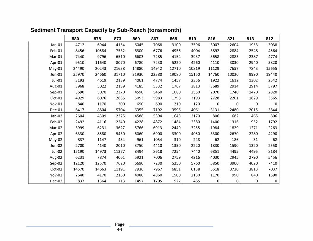
Page 44
Sediment Transport Capacity by Sub-Reach (tons/month) 880 878 873 869 867 868 819 816 821 813 812
Jan‐01 4712 6944 4154 6045 7068 3100 3596 3007 2604 1953 3038Feb‐01 8456 10584 7532 6300 6776 4956 4004 3892 2884 2548 4564Mar‐01 7440 9796 6510 6603 7285 4154 3937 3658 2883 2387 4774Apr‐01 9510 11640 8070 6780 7230 5220 4260 4110 3030 2940 5820May‐01 24490 20243 21638 14880 14942 12710 10819 11129 7657 7843 15655Jun‐01 35970 24660 31710 21930 22380 19080 15150 14760 10020 9990 19440Jul‐01 3193 4619 2139 4061 4774 1457 2356 1922 1612 1302 2542Aug‐01 3968 5022 2139 4185 5332 1767 3813 3689 2914 2914 5797Sep‐01 3690 5070 2370 4590 5460 1680 2550 2070 1740 1470 2820Oct‐01 4929 6076 2635 5053 5983 1798 3193 2728 2201 1829 3565Nov‐01 840 1170 300 690 690 210 120 0 0 0 0Dec‐01 6417 8804 5704 6355 7192 3596 4061 3131 2480 2015 3844Jan‐02 2604 4309 2325 4588 5394 1643 2170 806 682 465 806Feb‐02 2492 4116 2240 4228 4872 1484 2380 1400 1316 952 1792Mar‐02 3999 6231 3627 5766 6913 2449 3255 1984 1829 1271 2263Apr‐02 6330 8580 5430 6060 6900 3300 4050 3300 2670 2280 4290May‐02 837 1147 434 961 1054 310 248 62 186 31 62Jun‐02 2700 4140 2010 3750 4410 1350 2220 1830 1590 1320 2550Jul‐02 15190 14973 11377 8494 8618 7254 7440 6851 4495 4495 8184Aug‐02 6231 7874 4061 5921 7006 2759 4216 4030 2945 2790 5456Sep‐02 12120 12570 7620 6690 7230 5250 5760 5850 3900 4020 7410Oct‐02 14570 14663 11191 7936 7967 6851 6138 5518 3720 3813 7037Nov‐02 2640 4170 2160 4080 4860 1500 2130 1170 990 840 1590Dec‐02 837 1364 713 1457 1705 527 465 0 0 0 0
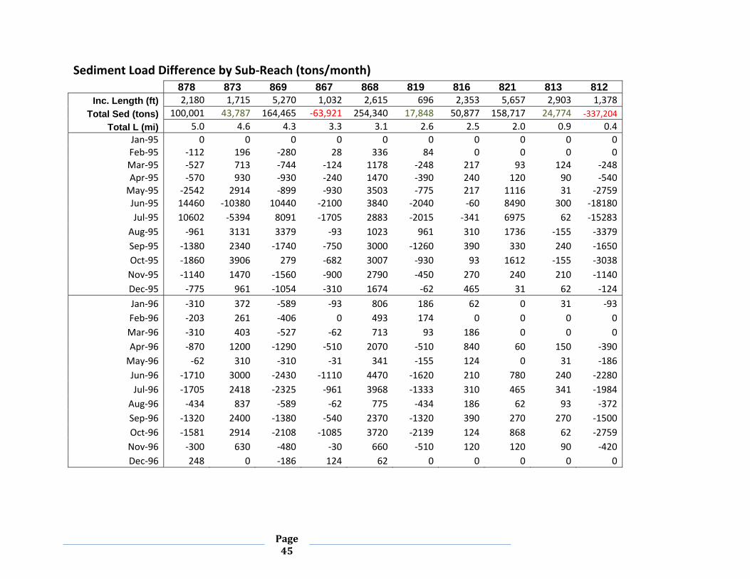
Page 45
Sediment Load Difference by Sub‐Reach (tons/month)878 873 869 867 868 819 816 821 813 812
Inc. Length (ft) 2,180 1,715 5,270 1,032 2,615 696 2,353 5,657 2,903 1,378Total Sed (tons) 100,001 43,787 164,465 ‐63,921 254,340 17,848 50,877 158,717 24,774 ‐337,204
Total L (mi) 5.0 4.6 4.3 3.3 3.1 2.6 2.5 2.0 0.9 0.4Jan‐95 0 0 0 0 0 0 0 0 0 0Feb‐95 ‐112 196 ‐280 28 336 84 0 0 0 0Mar‐95 ‐527 713 ‐744 ‐124 1178 ‐248 217 93 124 ‐248Apr‐95 ‐570 930 ‐930 ‐240 1470 ‐390 240 120 90 ‐540May‐95 ‐2542 2914 ‐899 ‐930 3503 ‐775 217 1116 31 ‐2759Jun‐95 14460 ‐10380 10440 ‐2100 3840 ‐2040 ‐60 8490 300 ‐18180Jul‐95 10602 ‐5394 8091 ‐1705 2883 ‐2015 ‐341 6975 62 ‐15283Aug‐95 ‐961 3131 3379 ‐93 1023 961 310 1736 ‐155 ‐3379Sep‐95 ‐1380 2340 ‐1740 ‐750 3000 ‐1260 390 330 240 ‐1650Oct‐95 ‐1860 3906 279 ‐682 3007 ‐930 93 1612 ‐155 ‐3038Nov‐95 ‐1140 1470 ‐1560 ‐900 2790 ‐450 270 240 210 ‐1140Dec‐95 ‐775 961 ‐1054 ‐310 1674 ‐62 465 31 62 ‐124Jan‐96 ‐310 372 ‐589 ‐93 806 186 62 0 31 ‐93Feb‐96 ‐203 261 ‐406 0 493 174 0 0 0 0Mar‐96 ‐310 403 ‐527 ‐62 713 93 186 0 0 0Apr‐96 ‐870 1200 ‐1290 ‐510 2070 ‐510 840 60 150 ‐390May‐96 ‐62 310 ‐310 ‐31 341 ‐155 124 0 31 ‐186Jun‐96 ‐1710 3000 ‐2430 ‐1110 4470 ‐1620 210 780 240 ‐2280Jul‐96 ‐1705 2418 ‐2325 ‐961 3968 ‐1333 310 465 341 ‐1984Aug‐96 ‐434 837 ‐589 ‐62 775 ‐434 186 62 93 ‐372Sep‐96 ‐1320 2400 ‐1380 ‐540 2370 ‐1320 390 270 270 ‐1500Oct‐96 ‐1581 2914 ‐2108 ‐1085 3720 ‐2139 124 868 62 ‐2759Nov‐96 ‐300 630 ‐480 ‐30 660 ‐510 120 120 90 ‐420Dec‐96 248 0 ‐186 124 62 0 0 0 0 0

Page 46
Sediment Load Difference by Sub‐Reach (tons/month)878 873 869 867 868 819 816 821 813 812
Jan‐97 155 62 ‐186 93 93 0 0 0 0 0Feb‐97 ‐168 364 ‐252 84 196 56 0 0 0 0Mar‐97 ‐186 217 ‐372 0 465 155 0 0 0 0Apr‐97 ‐480 750 ‐690 ‐120 1020 ‐390 270 90 120 ‐300May‐97 ‐1395 1767 ‐1643 ‐713 2945 ‐1426 465 341 310 ‐1674Jun‐97 ‐1020 1530 ‐1290 ‐390 2160 ‐540 210 240 180 ‐750Jul‐97 ‐1953 3720 ‐744 ‐837 3410 ‐682 31 1302 31 ‐2852Aug‐97 ‐1550 4061 1147 ‐527 837 ‐992 ‐744 2418 ‐744 ‐6913Sep‐97 20820 ‐14550 16230 ‐2940 6510 1080 840 11490 1380 ‐21120Oct‐97 ‐1643 2511 ‐2294 ‐1054 4061 ‐1457 682 403 372 ‐1767Nov‐97 ‐1950 2880 ‐2010 ‐1140 4530 ‐1290 840 450 420 ‐1560Dec‐97 ‐2232 3038 ‐1426 ‐992 4216 ‐961 682 651 434 ‐1860Jan‐98 ‐2356 3007 ‐1302 ‐961 4154 ‐837 1147 496 496 ‐1302Feb‐98 ‐1624 1932 ‐2296 ‐868 3724 ‐448 1568 112 280 0Mar‐98 ‐2294 2883 ‐1767 ‐992 4216 ‐527 1519 341 496 ‐558Apr‐98 6420 ‐3570 9210 450 2340 2550 2040 2880 540 ‐3270May‐98 19933 ‐16771 22072 ‐372 5735 4681 1674 8463 1147 ‐13237Jun‐98 ‐450 2700 3330 180 1170 1830 900 1200 360 ‐2250Jul‐98 ‐992 1705 ‐1240 ‐372 2108 ‐341 341 186 155 ‐527Aug‐98 25823 ‐18476 19158 ‐5642 8525 5363 868 14632 837 ‐30938Sep‐98 3900 ‐810 5850 ‐300 2160 1590 690 3390 240 ‐5340Oct‐98 ‐403 1271 ‐589 ‐124 899 ‐93 186 31 31 ‐217Nov‐98 ‐1980 3060 ‐1530 ‐990 4020 ‐660 1050 420 360 ‐1320Dec‐98 ‐2356 3069 ‐217 ‐806 3472 ‐403 558 868 372 ‐2294
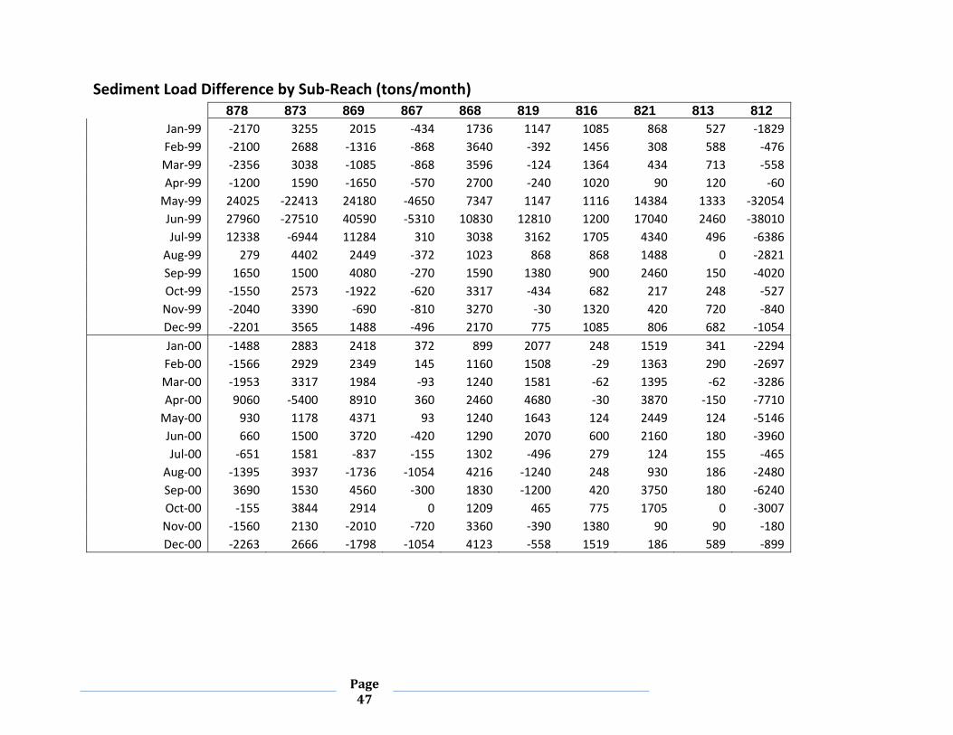
Page 47
Sediment Load Difference by Sub‐Reach (tons/month)878 873 869 867 868 819 816 821 813 812
Jan‐99 ‐2170 3255 2015 ‐434 1736 1147 1085 868 527 ‐1829Feb‐99 ‐2100 2688 ‐1316 ‐868 3640 ‐392 1456 308 588 ‐476Mar‐99 ‐2356 3038 ‐1085 ‐868 3596 ‐124 1364 434 713 ‐558Apr‐99 ‐1200 1590 ‐1650 ‐570 2700 ‐240 1020 90 120 ‐60May‐99 24025 ‐22413 24180 ‐4650 7347 1147 1116 14384 1333 ‐32054Jun‐99 27960 ‐27510 40590 ‐5310 10830 12810 1200 17040 2460 ‐38010Jul‐99 12338 ‐6944 11284 310 3038 3162 1705 4340 496 ‐6386Aug‐99 279 4402 2449 ‐372 1023 868 868 1488 0 ‐2821Sep‐99 1650 1500 4080 ‐270 1590 1380 900 2460 150 ‐4020Oct‐99 ‐1550 2573 ‐1922 ‐620 3317 ‐434 682 217 248 ‐527Nov‐99 ‐2040 3390 ‐690 ‐810 3270 ‐30 1320 420 720 ‐840Dec‐99 ‐2201 3565 1488 ‐496 2170 775 1085 806 682 ‐1054Jan‐00 ‐1488 2883 2418 372 899 2077 248 1519 341 ‐2294Feb‐00 ‐1566 2929 2349 145 1160 1508 ‐29 1363 290 ‐2697Mar‐00 ‐1953 3317 1984 ‐93 1240 1581 ‐62 1395 ‐62 ‐3286Apr‐00 9060 ‐5400 8910 360 2460 4680 ‐30 3870 ‐150 ‐7710May‐00 930 1178 4371 93 1240 1643 124 2449 124 ‐5146Jun‐00 660 1500 3720 ‐420 1290 2070 600 2160 180 ‐3960Jul‐00 ‐651 1581 ‐837 ‐155 1302 ‐496 279 124 155 ‐465Aug‐00 ‐1395 3937 ‐1736 ‐1054 4216 ‐1240 248 930 186 ‐2480Sep‐00 3690 1530 4560 ‐300 1830 ‐1200 420 3750 180 ‐6240Oct‐00 ‐155 3844 2914 0 1209 465 775 1705 0 ‐3007Nov‐00 ‐1560 2130 ‐2010 ‐720 3360 ‐390 1380 90 90 ‐180Dec‐00 ‐2263 2666 ‐1798 ‐1054 4123 ‐558 1519 186 589 ‐899

Page 48
Sediment Load Difference by Sub‐Reach (tons/month)878 873 869 867 868 819 816 821 813 812
Jan‐01 ‐2232 2790 ‐1891 ‐1023 3968 ‐496 589 403 651 ‐1085Feb‐01 ‐2128 3052 1232 ‐476 1820 952 112 1008 336 ‐2016Mar‐01 ‐2356 3286 ‐93 ‐682 3131 217 279 775 496 ‐2387Apr‐01 ‐2130 3570 1290 ‐450 2010 960 150 1080 90 ‐2880May‐01 4247 ‐1395 6758 ‐62 2232 1891 ‐310 3472 ‐186 ‐7812Jun‐01 11310 ‐7050 9780 ‐450 3300 3930 390 4740 30 ‐9450Jul‐01 ‐1426 2480 ‐1922 ‐713 3317 ‐899 434 310 310 ‐1240Aug‐01 ‐1054 2883 ‐2046 ‐1147 3565 ‐2046 124 775 0 ‐2883Sep‐01 ‐1380 2700 ‐2220 ‐870 3780 ‐870 480 330 270 ‐1350Oct‐01 ‐1147 3441 ‐2418 ‐930 4185 ‐1395 465 527 372 ‐1736Nov‐01 ‐330 870 ‐390 0 480 90 120 0 0 0Dec‐01 ‐2387 3100 ‐651 ‐837 3596 ‐465 930 651 465 ‐1829Jan‐02 ‐1705 1984 ‐2263 ‐806 3751 ‐527 1364 124 217 ‐341Feb‐02 ‐1624 1876 ‐1988 ‐644 3388 ‐896 980 84 364 ‐840Mar‐02 ‐2232 2604 ‐2139 ‐1147 4464 ‐806 1271 155 558 ‐992Apr‐02 ‐2250 3150 ‐630 ‐840 3600 ‐750 750 630 390 ‐2010May‐02 ‐310 713 ‐527 ‐93 744 62 186 ‐124 155 ‐31Jun‐02 ‐1440 2130 ‐1740 ‐660 3060 ‐870 390 240 270 ‐1230Jul‐02 217 3596 2883 ‐124 1364 ‐186 589 2356 0 ‐3689Aug‐02 ‐1643 3813 ‐1860 ‐1085 4247 ‐1457 186 1085 155 ‐2666Sep‐02 ‐450 4950 930 ‐540 1980 ‐510 ‐90 1950 ‐120 ‐3390Oct‐02 ‐93 3472 3255 ‐31 1116 713 620 1798 ‐93 ‐3224Nov‐02 ‐1530 2010 ‐1920 ‐780 3360 ‐630 960 180 150 ‐750Dec‐02 ‐527 651 ‐744 ‐248 1178 62 465 0 0 0

C h e r r y C r e e k S e d i m e n t a t i o n S t u d y R e s e r v o i r t o P i n e L a n e
S c e n a r i o D e v e l o p m e n t a n d E v a l u a t i o n
May 2011 Prepared for: Southeast Metropolitan Stormwater Authority 76 Inverness Drive Englewood, Colorado Submitted to: Ms. Molly Trujillo, P.E. Prepared by:
GK COTTON CONSULTING, INC 10290 S. Progress Way, #205 PO Box 1060 Parker, CO 80134-1060
GEORGE K COTTON CONSULTING, INC
HYDROLOGIC ENGINEERING AND DESIGN
SCENARIO DEVELOPMENT AND EVALUATION 2 | P A G E
C H E R RY C R E E K S E D I M E N TAT I O N S T U DY
SCENARIO DEVELOPMENT AND EVALUATION
Table of Contents
Introduction............................................................................................................................. 3
Design Flows ........................................................................................................................... 3
Analysis of SMWSA Master Plan ....................................................................................................... 3
Analysis of Major Drainageway Master Plan .................................................................................... 6
CCBWQA Dominant Discharge .......................................................................................................... 9
Recommended Flows ....................................................................................................................... 9
Channel Design Scenarios ...................................................................................................... 11
Equilibrium Index Method .............................................................................................................. 11
Selected Proxy Reach ..................................................................................................................... 12
Scenario #1 .................................................................................................................................... 12
Scenario #2 .................................................................................................................................... 12
Scenario #3 .................................................................................................................................... 13
Discussion of Scenarios #2 and #3 .................................................................................................. 14
Summary and Findings .......................................................................................................... 15
References ............................................................................................................................. 16
Appendix A. Stream Channel Stability Calculations ................................................................ 17
Appendix B. Stability Index Method ....................................................................................... 23
Gradually Varied Flow .................................................................................................................... 23
Prototype/Model Similitude .......................................................................................................... 23 Effect of Roughness ............................................................................................................................................ 24 Scaling of Sediment Transport ............................................................................................................................ 25
Alluvial Channel Scaling Relationships ............................................................................................ 25
Stable Channel Assessment – Equilibrium Relationships ................................................................. 27 Lane Relationship ‐ Enhanced ............................................................................................................................. 27 Equilibrium Index Approach ............................................................................................................................... 27

GEORGE K COTTON CONSULTING, INC
HYDROLOGIC ENGINEERING AND DESIGN
SCENARIO DEVELOPMENT AND EVALUATION 3 | P A G E
INTRODUCTION
This paper discusses possible scenarios for channel design that are based on an assessment of equilibrium analysis of the Cherry Creek for a study reach that extends from the confluence of Baldwin Gulch (Pine Lane bridge over the Cherry Creek) to the Piney Creek confluence (southern boundary of Cherry Creek State Park). The analysis uses channel geometry, mean bed material size, and stream gradient data that were compiled for the sedimentation study (see preceding study papers). In this paper, new scaled 2-year flows for sub-reaches of the study reach are developed. The development of these discharges is discussed in some detail and is admittedly approximate but provide sufficient detail for this level of analysis. The hydrology of the Cherry Creek is complex due to importation of a substantial amount of water into the Cherry Creek basin to meet the growth in water demand by developing communities within the basin. The Cherry Creek alluvial aquifers play an important role in recycling the portion of this imported water permitted under Colorado water law.
The losing nature of the Cherry Creek through the study reach is challenging for channel design because it diminishes that capacity of stream to transport the natural supply of sediment that is delivered to the stream by the watershed. The sediment budget (see study paper “Sediment Budget”) found that most sub-reaches in the study reach will have sedimentation. However, maintaining sediment transport is desirable because of the maintenance associated with removing sediment deposits and the increased risks due to loss of channel capacity.
The upper sub-reach is estimated to be stable and so serves as the proxy reach for the evaluation of sediment equilibrium in the lower reaches. A method of equilibrium analysis is used which scales the discharge, material size, stream gradient and sediment transport relative to proxy reach. Three scenarios were developed based on the objective of transporting a uniform sediment load through the study reach. Stream reaches with a uniform transport rate through all of the sub-reaches will not be as prone to scour and deposition. The recommended scenario comports with current channel reclamation projects that have already been constructed but does not convey the entire basin sediment load. As a result, sediment deposition appears to be likely near the Arapahoe / Douglas County line (sub-reach 873) further analysis will be required to determine the most likely locations for deposition.
DESIGN FLOWS
The long-term hydrology of the Cherry Creek in the sedimentation study reach (Pine Lane to the Reservoir) is that of a losing reach, according to models that take into consideration water supply operations. It is likely that water diversion from the alluvial aquifer affects more frequent flood hydrology and channel forming discharges. Three hydrology studies are reviewed: the SMWSA Master Plan, the Major Drainageway Planning Study, and the CCBWQA phosphorus model.
ANALYSIS OF SMWSA MASTER PLAN
In 2007, the South Metro Water Supply Authority published its master plan for water supply development. SMWSA is an umbrella for 13 water providers, most of which are within the Cherry Creek basin. More than 80% of the SMWSA water supply is used within the Cherry Creek basin. Future storage of renewable water supplies by all of the SMWSA water providers occurs at the new Rueter-Hess reservoir, which is also within the Cherry Creek basin.

GEORGE K COTTON CONSULTING, INC
HYDROLOGIC ENGINEERING AND DESIGN
SCENARIO DEVELOPMENT AND EVALUATION 4 | P A G E
Figure 1 (below) from the SMWSA Master Plan shows the breakdown of water supplies over the planning horizon. Table 1 provides the same information as the graph and also back casts to the year 2000.
Figure 1. Taken from SMWSA Master Plan 2007
Table 1. SMWSA Water Sources over planning horizon
Year Renewable Supply
Surface Supply
Renewable Buffer
Ground Water
Recap / Return
Alluvial (water rights)
Total
2000 0 500 0 42220 3000 3500 49220 2010 4000 24300 400 25900 11900 4300 708002020 17800 27100 1780 19800 20800 5100 923802030 32900 25100 3290 14900 24000 5100 105290
Buildout 43400 25100 4340 14900 28100 5100 120940
Most of the water supply for the SMWSA water providers comes from imported sources. SMWSA’s goal is to shift from a heavy dependence on non-renewable groundwater to renewable water supplies by acquiring surface water rights in other basins and transporting this supply to the SMWSA service area and then to each service provider. This will require the development of existing water rights (called surface supply), then acquiring and developing new water rights (called renewable supply). This will permit ground water use to decline. To account for uncertainty in this process, the master plan includes a renewable buffer that is equal to 10% of the estimated required renewable supply.

GEORGE K COTTON CONSULTING, INC
HYDROLOGIC ENGINEERING AND DESIGN
SCENARIO DEVELOPMENT AND EVALUATION 5 | P A G E
A second source of water supply for SMWSA water providers comes from the recapture of flows or return flows. These flows will largely be recovered through alluvial wells. Also, most of the surface water rights on Cherry Creek are diverted through alluvial wells.
So, water supply for SMWSA water providers can be aggregated into two classes: imported supplies (renewable, surface, and groundwater), and alluvial (recapture / return and alluvial water rights). I estimate that on an annual basis about 44% of the total supply will be returned (assuming that 42% of the supply is for domestic use and 58% is for irrigation, with 10% consumption of domestic water and 90% consumption of irrigation). Table 2 provides an estimate of the un-diverted alluvial flow (both flow in the alluvial aquifers and in surface streams), where the un-diverted alluvial flow is equal to 44% of the total supply minus the diverted alluvial flow. These data are shown graphically in Figure 2.
Table 2. Estimate of Un-Diverted Alluvial Flows within SMWSA
Year Total Diverted Alluvial
Imported Flows
Un‐Diverted Alluvial
2000 49220 6500 42720 14960 2010 70800 16200 54600 14669 2020 92380 25900 66480 14378 2030 105290 29100 76190 16806
Buildout 120940 33200 87740 19530
Figure 2. SMWSA Master Plan Water Supply Breakdown

GEORGE K COTTON CONSULTING, INC
HYDROLOGIC ENGINEERING AND DESIGN
SCENARIO DEVELOPMENT AND EVALUATION 6 | P A G E
In 2000, 82% of the SMWSA water providers were associated with the Cherry Creek basin. Using sub-reach 880 in the CCBWQA model (Parker, CO) as a point of reference the SMWSA master plan estimates that 12,300 ac-ft of un-diverted alluvial flow occurred at this point in the Cherry Creek. This compares with 11,700 ac-ft estimated by the CCBWQA model. In addition, the CCBWQA model estimates a reach flow loss of 2,500 ac-ft compared to SMWSA estimate of 5,300 ac-ft.
Recovery of flows will increase steadily, which will increase the total diverted alluvial flow in the Cherry Creek. In 2000, only about 6.1% of the total supply was recovered. SMWSA estimates that in 2010, 16.8% was recovered and that by 2020 22.5% will be recovered, which will be close to the maximum expected recovery that will be achieved at build out (23.2%). The result is that un-diverted alluvial flows remain essentially unchanged even as water supply is dramatically increased to the Cherry Creek basin. Of all of the sources of water supply for water providers in SMWSA, recovered flows are probably one of the least difficult to acquire administratively and the least costly to deliver.
ANALYSIS OF MAJOR DRAINAGEWAY MASTER PLAN
The “Cherry Creek Major Drainageway Planning Study” was prepared in 2002 and provides an estimate of the flood hydrology for existing and future conditions in the basin. This hydrology deals directly with the main effect of rural to urban land use change, which is the increase in impervious area and the resulting increase in runoff volume. This is a condition that is not addressed by the SMWSA master plan for the reason that stormwater runoff is considered a minor and unreliable source of water. This may not be entirely true. From 1985 to 2010, basin imperviousness has increased for 13% to 23% and will continue to increase at the rate of 1% for every 11,600 housing units built in the basin. Runoff from these impervious areas ultimately connects to the Cherry Creek, where it may be diverted for water supply as long as overall basin yield from Cherry Creek tends to maintain the historical average.
Urban runoff enters the Cherry Creek via storm drainage outfalls and tributary drainageways. It appears that alluvial pumping very quickly captures minor runoff. So CCBWQA estimates of base flow, which comport with SMWSA planning, indicate that the “Cherry Creek Major Drainageway Planning Study” probably over estimates frequent floods such as the 2-year.
Estimates of less frequent floods are intended to be conservative and are intended to provide a prudent means of delineating flood hazards. All of the jurisdictions in the Cherry Creek carefully administer floodplain regulations and development standards that should ensure that the future floods are less severe than are predicted by the planning study. Tables 3 and 4 summarize flood hydrology data from the “Cherry Creek Major Drainageway Planning Study”.

GEORGE K COTTON CONSULTING, INC
HYDROLOGIC ENGINEERING AND DESIGN
SCENARIO DEVELOPMENT AND EVALUATION 7 | P A G E
Table 3. Peak Flow Summary - Sedimentation Study Reach / Existing Conditions
EXISTING CONDITIONS (CFS) Sub‐Rch Q002 Q005 Q010 Q025 Q050 Q100 880 1555 4441 8100 16039 24040 39785 878 1564 4454 8115 16072 24058 39835 873 1552 4423 8087 16000 23968 39636 869 1557 4431 8092 16028 23975 39622 867 1563 4438 8102 16056 23980 39630 868 1562 4430 8095 16042 23948 39557 819 1791 5021 8954 17866 27045 43625 816 1764 4980 8915 17772 26832 43272 821 1759 4971 8906 17751 26777 43170 813 1767 4984 8921 17795 26814 43213 812 1769 4986 8921 17798 26812 43217 811 1769 4986 8921 17798 26811 43217
Table 4. Peak Flow Summary - Sedimentation Study Reach / Future Conditions
FUTURE CONDITIONS (CFS) Sub‐Rch Q002 Q005 Q010 Q025 Q050 Q100 880 3294 7000 10939 19599 28168 43246 878 3341 7097 11026 19705 28303 43338 873 3330 7121 11033 19702 28238 43215 869 3347 7170 11083 19762 28272 43263 867 3361 7218 11128 19824 28310 43301 868 3360 7221 11136 19820 28287 43244 819 3949 8389 12825 22573 32353 48250 816 3882 8298 12731 22409 32042 47891 821 3894 8324 12784 22485 32036 47864 813 3915 8356 12829 22570 32100 47897 812 3919 8361 12836 22590 32097 47876 811 3919 8361 12836 22590 32095 47872

GEORGE K COTTON CONSULTING, INC
HYDROLOGIC ENGINEERING AND DESIGN
SCENARIO DEVELOPMENT AND EVALUATION 8 | P A G E
One approach to using the planning study flood hydrology would be to scale the existing 2-year flood peak for sub-reach 880 by the flow volume ratios (sub-reach volume divided by sub-reach 880 volume) as computed by the CCBWQA model (Table 5). Using this approach, the 2-year existing and future conditions would be as shown in Table 6.
Table 5. Sub-Reach Flow Scaling following based on volume (CCBWQA model)
Sub-Reach 880 878 873 869 867 868
Volume (ac-ft) 76,368 74,567 72,358 67,681 65,061 65,718Flow Scaling 100.0% 97.6% 94.7% 88.6% 85.2% 86.1%
Sub-Reach 819 816 821 813 812 811
Volume (ac-ft) 70,918 61,328 62,880 59,287 56,555 52,232Flow Scaling 92.9% 80.3% 82.3% 77.6% 74.1% 68.4%
Table 6. “Cherry Creek Major Drainageway Planning Study” Scaled 2-year flows
Scaling Existing Conditions Future Conditions
Sub‐Rch Factor Original Scaled Ratio Original Scaled Ratio 880 100.0% 1555 1555 100.0% 3294 3294 100.0%878 97.6% 1564 1518 97.0% 3341 3215 96.2%873 94.7% 1552 1473 94.9% 3330 3119 93.7%869 88.6% 1557 1378 88.5% 3347 2918 87.2%867 85.2% 1563 1325 84.8% 3361 2806 83.5%868 86.1% 1562 1339 85.7% 3360 2836 84.4%819 92.9% 1791 1445 80.7% 3949 3060 77.5%816 80.3% 1764 1249 70.8% 3882 2645 68.1%821 82.3% 1759 1280 72.8% 3894 2711 69.6%813 77.6% 1767 1207 68.3% 3915 2556 65.3%812 74.1% 1769 1152 65.1% 3919 2441 62.3%811 68.4% 1769 1064 60.1% 3919 2253 57.5%

GEORGE K COTTON CONSULTING, INC
HYDROLOGIC ENGINEERING AND DESIGN
SCENARIO DEVELOPMENT AND EVALUATION 9 | P A G E
CCBWQA DOMINANT DISCHARGE
The dominant discharge for a stream reach is the product of the probability of a stream discharge multiplied by the sediment load in the reach. This probability approach places a higher weighting on frequent stream flows and lower weighting of rare stream flows. The discharge associated with the maximum weighted sediment loading is referred to as the dominant discharge. This method was used to identify the dominant discharge in the sub-reaches of the study reach over the eight year CCBWQA model simulation. Figure 3 shows the calculation results graphically.
Table 7. Sub-Reach dominant discharges (CCBWQA model)
Sub-Reach 880 878 873 869 867 868
Dominant Q (ac-ft/mo) 1080 880 960 550 500 800
Sub-Reach 819 816 821 813 812 811
Dominant Q (ac-ft/mo) 550 550 500 600 500 n/c
The weighting of more frequent sediment loads follows a normal pattern, which rises steadily to a peak
value. While there is a distinct peak in weighted sediment loads for each sub-reach, the less frequent sediment loads don’t decline and can reach values that equal or exceed the first peak. This may be a product of the short period of simulation or the complex way that water is routed and diverted from the Cherry Creek.
RECOMMENDED FLOWS
While scaling of flows based on volume is admittedly a very approximate approach it has the advantage of comporting to major drainageway planning and to the losing nature of reach as shown in the CCBWQA model and SMWSA master planning. In the long run, we recommend that the UDSWM model that was used for major drainageway planning be converted to EPA-SWMM. In this way, additional modeling elements found in the CCBWQA analysis could be included. EPA-SWMM has similar routines to those developed for the CCBWQA model (for example, alluvial groundwater flow simulation), so the model conversion could draw on data and calibration work already conducted by CCBWQA.
For the time being, using scaled 2-year existing-conditions flows from the major drainageway planning study is recommended (green highlighted column in Table 6). Use of future flows is not recommended because the SMWSA planning does not show a future increase in un-diverted alluvial flows.

Figure 3 Shows plots of dominant discharge calculation as computed by sub-reach for the CCBWQA simulation. The vertical lines show the approximate location of the first peak in weighted sediment loading, i.e. the dominant discharge for the sub-reach (ac-ft/month). The vertical axis is the probability weighted sediment transport in tons.

GEORGE K COTTON CONSULTING, INC
HYDROLOGIC ENGINEERING AND DESIGN
SCENARIO DEVELOPMENT AND EVALUATION 11 | P A G E
CHANNEL DESIGN SCENARIOS
In most streams, water discharge and sediment load gradually increase. In response, channel size tends to increase and channel gradient may slightly decrease. In streams with heavy flow diversion, sediment transport capacity is quickly lost as discharge is lost. This results in sediment deposition and a decrease in channel size. Deposition tends to be a chronic problem and sediment will gradually diminish channel capacity over many years. This will necessitate periodic removal of sediment from the channel. Therefore, it is desirable to maintain sediment transport capacity, if possible, by countering the loss of discharge with increased stream power.
Three scenarios are evaluated here with the objective of maximizing the transport of sediment. The first scenario looks at minimal improvement of existing channel conditions; the second scenario looks at channel improvements similar to the type of stream reclamation projects currently being constructed in the reach; and the third scenario mimics the form of a stable reach of the Cherry Creek. The scenarios are not mutually exclusive but could be combined as needed to take best advantage of opportunities for channel improvement on the Cherry Creek.
EQUILIBRIUM INDEX METHOD
The equilibrium index method is based on fundamental scaling relationships for basic stream cross section properties (i.e., material size, stream discharge, sediment transport and stream gradient) that are widely used in geomorphology, stream assessment and channel restoration design. The method uses Griffith’s (2003) derivation of Leopold and Maddock’s (1953) empirical equations for stream scaling (see Appendix B). Sediment transport is added in the form of a power function equation that is based on the calibrated Engelund-Hansen equation that was developed for the Cherry Creek.
The resulting equation is referred to as the equilibrium index, IE, where:
IE = Qr
h Sr
Gbr drg
Qr is the dimensionless steam discharge; Sr is the dimensionless steam gradient; Gbr is the dimensionless steam discharge; and, dr is the dimensionless mean sediment size h and g are scaling exponents that are derived from hydraulic and sediment transport formulas Note: The subscript “r” refers to the ratio of reach variable to proxy reach variable.
The spreadsheet computes uniform flow in a channel section that is defined by a depth versus topwidth rating. Sediment transport is computed for the active, un-vegetated portion of the channel and the vegetated portions of the active channel and overbanks. The stream discharges are the selected design discharges, the material property is the average sediment size, and reach gradients are taken from topographic maps.
When the equilibrium index is near 1.0 then the stream conditions are balanced between the stream’s power (numerator) and the work needed for sediment transport (denominator). The equilibrium equation cannot be solved directly since the each variable interacts with the others. The solution is obtained by trial and error. In the spread sheet, variables that can potentially change have yellow cells, while cells that are

GEORGE K COTTON CONSULTING, INC
HYDROLOGIC ENGINEERING AND DESIGN
SCENARIO DEVELOPMENT AND EVALUATION 12 | P A G E
computed are shown in light purple and scaling variables are shown in blue. The final results of each scenario calculation are provided in Appendix A.
SELECTED PROXY REACH
The most upstream sub-reach 880 was found to be a stable stream reach of the Cherry Creek. This reach was used as the upstream boundary for the sediment budget analysis. Sub-reach 880 characteristics (geometry, mean sediment size, and stream gradient) that were used for sediment budget analysis were also used as proxy reach characteristics.
SCENARIO #1
This scenario develops a uniform rate of sediment transport with minimal modification to the existing stream channel. Uniform sediment transport conditions were obtained by adjusting the stream grade and the stream active channel width until sediment transport capacity equaled that of the upstream proxy reach. The largest difference in sediment transport capacity existing at sub-reach 869 (“17 Mile House”reach), which is an improved reach of the Cherry Creek (completed in 2006), and the two downstream sub-reaches that are above the Happy Canyon Creek confluence (stream reaches managed by the Parker/Jordan Metro District).
It is expected that sub-reach channel gradients would adjust over time to regain transport capacity. Existing sub-reach gradients vary from 0.192% (the as-built profile for sub-reach 869) to 0.40% near Arapahoe Road. The adjusted gradient was computed to be 0.395%. As a result, the active channel width was calculated varies between about 18 feet to 50 feet.
The main problem with this scenario is the low width/depth ratios for the active channel. When a sand bed channel is relatively narrow, there is a strong potential for low-flow incisement. This has been a chronic problem for reaches of the Cherry Creek since the increase base flow that began in the early 1990’s. A second problem is the irregularity of active channel width and floodplain width. This may be a secondary cause of low-flow incisement during larger flows because narrow stream reaches have higher active channel velocities.
This scenario shows that it is possible to carry the total sediment load through the lower reaches of the study reach. The reach geometry adjustments appear logical with stream generally increasing in width in the downstream direction. However, the change in width is very irregular due and is strongly influence by encroachment into the floodplain. The un-vegetated active channel width for sub-reach 812 (at Caley Avenue) is exceptionally narrow. During a large flood this sub-reach has would also have significant contraction scour.
SCENARIO #2
This scenario assumes that sub-reach channels below 17 Mile House will continue to be improved following guidance provided by major drainageway planning. As an approximation, scenario #2 assumes that these channel improvements will generally follow the form of the 17-Mile House stream reclamation (based on the project as-built plans).
The grade of the channel in sub-reach 869 was adjusted to match proxy reach sediment transport capacity. This would be an adjustment from a constructed grade of 0.192% to a gradient of 0.263%. This is slightly less than the total grade between riffle drop crests (0.36%), which would slightly affect the capacity of the low-flow channel but would probably not impact that stability of this reach.
The geometry of downstream sub-reaches was varied by adjusting the active channel width and channel grade to maintain a sediment transport capacity equal to that of the proxy reach. The channel banks are 4.0

GEORGE K COTTON CONSULTING, INC
HYDROLOGIC ENGINEERING AND DESIGN
SCENARIO DEVELOPMENT AND EVALUATION 13 | P A G E
feet high (topwidth B3 in the equilibrium calculation) and are assumed to maintain their height and slope as stream width increases. The unvegetated portion of the active channel was assumed to be 80% of the active channel width. The active channel width and channel grade were varied to maintain sediment transport capacity equal to that of the proxy reach. The result is an active channel at a nearly uniform gradient of 0.261% and an active width that is fairly uniform that slightly decreases in the downstream direction.
The Caley choke section (sub-reach 812) is relaxed for this scenario. At its 1-foot depth the cross section is about 80 feet wide, compared to the current width of only about 50 feet. The sensitivity of the cross section to encroachment is demonstrated by the need to widen the channel at its 6-foot (topwidth B4) from 173 feet to 486 feet.
The most significant problem with Scenario #2 is the lack of stream power. As a result, this alternative has low equilibrium indices, which are the result of the mild stream gradients. The channel section is fairly wide with a high width/depth ratio, which may result in areas of the cross section that have partial sedimentation (i.e. sand bars). Bars provide areas for the establishment of vegetation that can result in a narrowing of the unvegetated active channel and reduced sediment transport capacity. This would promote further deposition (increasing channel grade) until a balance between sediment transport and stream power is achieved.
As was anticipated by major drainageway planning, the difference in fall between the original channel grade and the improved channel grade would be accommodated by drop structures. Because deposition is likely for this scenario, it is desirable not to accumulate large differences in grade between drop structures, which would create the potential for large deposition areas between drop structures. This would not only affect channel capacity or but could also result in lateral instability.
A good guide to drop spacing is to follow the frequency of a riffle sequence with a small grade change at each riffle location. Riffle sequencing is roughly 2π times the channel width, which in natural stream can vary by nearly a factor of two. Therefore, construction of riffle sequences would only require on average of about 0.6 feet of drop per riffle to accommodate the potential grade difference that might be caused by sediment deposition. This would limit potential deposition to about 1.0 foot.
SCENARIO #3
Scenario #3 is an improved version of Scenario #1 that reduces the irregular variations in active channel width, while also adjusting stream gradient to maintain uniform sediment transport capacity. For this scenario, a small shallow active channel is incised into a wider channel floor. The channel is similar to the channel section of proxy reach near Pine Lane. The resulting channel gradient is similar to the grade computed for Scenario #1 (about 0.400% compared to 0.395%). The active channel is more uniform with an un-vegetated active channel width of about 10 to 12 feet. As with Scenario #1, the result is a small width to depth ratio (about 3), which makes the section vulnerable to low-flow incisement.
This scenario has the advantage of a much wider riparian zone compared to Scenario #2. At its 2-foot depth (topwidth B2), the channel has a riparian fringe (channel width minus the unvegetated active channel width) of about 152 feet compared to about 57 feet for Scenario #2. The active channel also carries less discharge (350 cfs compared to about 950 cfs for Scenario #2), which means that flow will be conveyed more frequently through the riparian zone. This provides a water quality benefit, since vegetated portions of the channel have a lower velocity that promote settling of sediment and allow nutrient exchange to plants.
In order to provide consistent sediment transport capacity, the channel section is more uniform and carries nearly constant topwidth at its 4-foot and 6-foot depths (350 feet and 486 feet, respectively). This would require eliminating floodplain encroachments within approximately a 500 foot width of the Cherry

GEORGE K COTTON CONSULTING, INC
HYDROLOGIC ENGINEERING AND DESIGN
SCENARIO DEVELOPMENT AND EVALUATION 14 | P A G E
Creek floodplain. This is not to say that the section needs to be completely prismatic, but the channel benefits from having relatively uniform cross section geometry. A related benefit of a wide vegetated overbank section is that the plant communities have more room to diversify.
This scenario has the advantage of having an equilibrium index that is close to 1.0. While there is still a deficit in stream power it is the lowest of all three scenarios. So it is the most likely scenario to transport the full upstream sediment load without excessive sedimentation during a large flood. The wider channel and steeper stream gradient are characteristic of the natural Cherry Creek stream environment. The low-flow channel would have capacity for current base flows but would require stabilization. Because there is less depth in the low channel there would also be a tendency for lateral migration within the channel overbank. So low-flow channel stabilization would need to include both vertical and lateral control structures.
DISCUSSION OF SCENARIOS #2 AND #3
Scenario #2 comports with most the channel improvements that have been constructed for the Cherry Creek to date. Its largest disadvantage is that it has a significant deficit in stream power relative to sediment transport capacity, and as a result, a potential for aggradation during larger flood events. Sediment balance for the reach indicates that there is enough sediment supplied that such aggradation would be possible. To understand the deposition pattern during larger flood events and determining the extent of problems for low flows will require further analysis that is based on sediment routing calculations. Sediment routing calculations can be conducted using HEC-RAS with sub-reach 880 at the supply reach.
Scenario #2 needs frequent grade control to absorb the difference between the design channel profile and the original stream gradient. Small drops that are based on a riffle sequence are recommended. With a limited drop height of about 0.6 feet and frequent drops of one about every 350 feet would provide consistent control of the channel grade. This approach recognizes that the biggest risk to stream channel stability is potential aggradation. Use of large drop structures risks a larger depth of deposition that would reduce waterway capacity and increase the potential for lateral migration. Smaller drops limit the sediment deposition to smaller depths that pose lower risks.
Scenario #3 is an alternative approach to the Cherry Creek that is closer to equilibrium. The major benefit is the increased size of the riparian zone and the associated water quality benefits of having more flow travel through vegetated areas of the channel. The additional overall channel width required for this scenario may not comport well with the history of encroachment within the study reach and lack of right-of-ways within the stream corridor. The smaller channel size and shallower embedment create the risk that the low-flow channel may shift within the overbank. So, control structures are needed for both vertical and horizontal channel stabilization.
While this analysis has focused on channel form associated with a minor 2-year flood, design must also consider major floods. Sediment loads created by a single large event can easily surpass the sediment load created by many years of transport by smaller flows. As a result, the low-flow channel section is vulnerable to being filled in or being out flanked during a major flood. Investigation is needed for any scenario to determine how likely an incised low-flow channel can survive a major flood. The investigation should address if there is a need for additional lateral stabilization of the active channel. It is recommended that the initial tool for these investigations be the one-dimensional moveable-bed model HEC-RAS.
Finally, it should be noted that Scenario #2 and #3 are not mutually exclusive. Since both scenarios have adequate sediment transport during low flow, they can be used as benefits different sub-reaches. Such mixing for stream cross sections would however make it even more important to evaluate channel behavior at transitions between sub-reaches during major floods using a moveable-bed model.

GEORGE K COTTON CONSULTING, INC
HYDROLOGIC ENGINEERING AND DESIGN
SCENARIO DEVELOPMENT AND EVALUATION 15 | P A G E
SUMMARY AND FINDINGS
1. Water supply development in the Cherry Creek basin results in the reach between Parker and Cherry Creek reservoir being a losing reach. It is expected that on average there will be about 32% less stream flow at the lower end of the study reach compared to inflow at the upper end.
2. An interim approach to the estimation of channel forming flows is proposed that scales the 2-year Major Drainageway Planning flow at sub-reach 880 according to the average loss rates calculated by the CCBWQA model for downstream sub-reaches.
3. It is recommended that a better model of minor floods and low-flows be developed that incorporates elements of the CCBWQA model (i.e. water storage in alluvial aquifers, aquifer flows, and pumping operations for water recovery). The new model should upgrade the Major Drainageway Planning hydrology model that is based on UDSWM to EPA-SWMM 4.
4. The upper sub-reach of the study area (sub-reach 880) was found to be stable and it is recommended as a reliable proxy reach for the estimation of incoming sediment supply to the study reach.
5. The equilibrium index method was applied to evaluate three channel design scenarios. It was found that recent improvements to the channel are not in equilibrium between sediment transport and stream power. This results in the potential for sediment deposition within the channel improvements. This aggradation is expected to be minor for 2-year flows and will require further investigation for major floods.
6. Scenarios #2 and #3 developed in this report can be mixed as needed to meet the needs of the corridor. Scenario #2 comports to prior design and major drainageway planning but may be vulnerable to significant aggradation during major floods. Scenario #3 has a cross-section geometry and profile grade that is similar to the original Cherry Creek channel. It has the advantage of creating a larger vegetated channel width, which would provide a significant water quality benefit.
7. It is highly recommended that detailed moveable-bed modeling be conducted for major floods in the study reach to determine the potential damage to downstream channel improvements.
8. A monitoring program for sedimentation and alluvial groundwater elevations should be started so that stream health can be routinely evaluated in light of very rapid changes occurring to the water supply within the basin and the extensive use of the alluvial aquifers as the means of recycling a large portion of that imported water supply as permitted by Colorado water law.
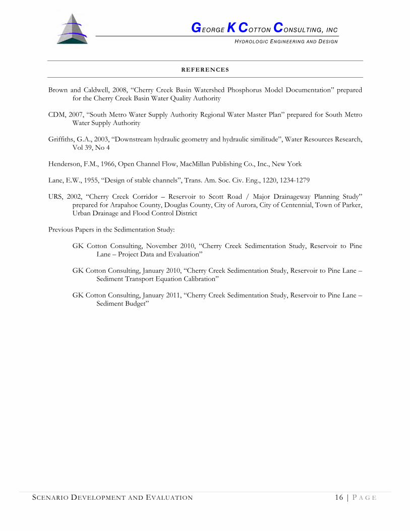
GEORGE K COTTON CONSULTING, INC
HYDROLOGIC ENGINEERING AND DESIGN
SCENARIO DEVELOPMENT AND EVALUATION 16 | P A G E
REFERENCES
Brown and Caldwell, 2008, “Cherry Creek Basin Watershed Phosphorus Model Documentation” prepared for the Cherry Creek Basin Water Quality Authority
CDM, 2007, “South Metro Water Supply Authority Regional Water Master Plan” prepared for South Metro Water Supply Authority
Griffiths, G.A., 2003, “Downstream hydraulic geometry and hydraulic similitude”, Water Resources Research, Vol 39, No 4
Henderson, F.M., 1966, Open Channel Flow, MacMillan Publishing Co., Inc., New York
Lane, E.W., 1955, “Design of stable channels”, Trans. Am. Soc. Civ. Eng., 1220, 1234-1279
URS, 2002, “Cherry Creek Corridor – Reservoir to Scott Road / Major Drainageway Planning Study” prepared for Arapahoe County, Douglas County, City of Aurora, City of Centennial, Town of Parker, Urban Drainage and Flood Control District
Previous Papers in the Sedimentation Study:
GK Cotton Consulting, November 2010, “Cherry Creek Sedimentation Study, Reservoir to Pine Lane – Project Data and Evaluation”
GK Cotton Consulting, January 2010, “Cherry Creek Sedimentation Study, Reservoir to Pine Lane – Sediment Transport Equation Calibration”
GK Cotton Consulting, January 2011, “Cherry Creek Sedimentation Study, Reservoir to Pine Lane – Sediment Budget”

GEORGE K COTTON CONSULTING, INC
HYDROLOGIC ENGINEERING AND DESIGN
SCENARIO DEVELOPMENT AND EVALUATION 17 | P A G E
APPENDIX A. STREAM CHANNEL STABILITY CALCULATIONS

Stream Channel Stability - REM-SSIPurpose: This workbook computes a stability index based on known stable
section as a proxy using L-M scaling and sediment transport scaling.REM-SSI is a program in the River Environment Modeling (REM) series.
References: Cotton, G.K., PE, 2010, "Stream process scaling and equilibrium index method" Griffiths, G.A., 2003, "Downstream hydraulic geometry and hydraulic similitude" Water Resources Research, Vol 39, No. 4.Leopold, L.B. and Maddock, T., 1953, "The hydraulic geometry of stream channelsand some physoiographic implications," USGS Prof. Paper 252.
Comments: Comments and questions on this workbook can be sent to:GK Cotton Consulting, Inc.10290 S. Progress Way, Ste 205Parker, Colorado 80134 email: [email protected]
Content: Reach- Tabulates the geometry, gradient, bed material size and discharge properties for mulitiple reaches.
SSI base- Computes the active channel velocity and sediment transport. The equilibrium index is computed based on an estimated properties of a prototype reach.
SSI Scenarios- Permits the user to adjust reach properties and develop analysis scenarios in a manner that drives the equilibrium index to equilibrium (IE = 1.0).
User Guide: Yellow cells indicate required input data for the workbook. Green cells indicate previous input values. Purple cells are computed dimensional values. Blue cells are dimensionless scaling values.
Project Information: Location:Calc by:
Last Revised:
Disclaimer:
Cherry Creek / Parker to Valley Country ClubGeorge Cotton, PEMay 3, 2011
George K Cotton Consulting, Inc. (aka GK Cotton Consulting) makes no warranties, express or implied, of merchantability or fitness for a particular purpose of this computer program. Anyone using this program assumes sole responsibility for the content of the files and shall, to the fullest extent permitted by law, indemnify, defend, and hold harmless GK Cotton Consulting from all claims, damages, losses, and expenses, including attorneys fees, arising out of or resulting therefrom. Any users of this program and the data contained therein agrees that the use of the program constitutes agreement to the above terms and conditions.

Stream Channel Stability - Reach DataLocation:Calc by: George Cotton, PE
Last Revised:Printed:
May 3, 2011May 4, 2011 13:59
Cherry Creek / Parker to Valley Country Club
Topwidth, ft
ReachReach
IDd50
(mm)Q2yr
(cfs)So
(ft/ft)Bunveg
(ft)B0
(ft)B1
(ft)B2
(ft)B3
(ft)B4
(ft)1 880 1.9 1555 0.00379 15.0 27.0 80.0 145.5 579.0 619.12 878 1.9 1518 0.00457 35.0 106.6 141.0 191.7 652.3 1070.93 873 1.9 1473 0.00472 34.0 35.0 44.0 479.0 504.0 610.04 869 1.9 1378 0.00383 34.0 35.0 37.0 115.1 355.5 387.75 867 1.9 1325 0.00438 34.0 35.0 53.9 84.1 287.5 319.26 868 1 9 1339 0 00400 34 0 35 0 50 7 78 8 135 0 736 5
p
6 868 1.9 1339 0.00400 34.0 35.0 50.7 78.8 135.0 736.57 819 1.9 1445 0.00358 38.0 39.0 58.7 166.1 176.7 187.38 816 1.2 1249 0.00343 25.0 40.8 104.0 275.6 599.8 807.39 821 1.2 1280 0.00333 25.0 123.0 201.6 371.1 471.6 487.5
10 813 1.2 1207 0.00403 25.0 123.0 172.2 371.1 473.5 485.411 812 1.2 1152 0.00388 24.0 25.0 51.0 84.8 113.1 172.612 811 1.2 1064 0.003882020
Depth, ft 0.0 0.0 1.0 2.0 4.0 6.0
Prototype 1.9 1555 0.00379 15.0 27.0 80.0 145.5 579.0 619.1
n-value Rating 0.025 0.311 0.311 0.146 0.076 0.061
Channel Geometry:
Gradation Data: Transport Equation:Grain siz
(mm) Overbank Active Up Valley0.25 15.1 2.5 4.2
0.5 41.5 14.0 12.61.0 72.7 42.1 28.9
% Finer
1.0 72.7 42.1 28.92.0 92.2 75.2 51.34.0 98.7 94.1 73.3 EH Scaling Factors:8.0 99.9 99.3 88.7 m1 m2
16.0 100.0 100.0 96.4 5.00 -0.50G = 2.3 2.2 3.2 e f g h
d50 = 0.6 1.2 1.9 1.1765 0.0588 0.2353 1.2941

Stream Channel Stability - Scenario #1 Uniform Sediment TransportLocation:Calc by:
Last Revised:Printed:
ReachQ2yr
(cfs)So
(ft/ft)Bunveg
(ft)
B0
(ft)B1
(ft)B2
(ft)B3
(ft)B4
(ft)d50
(mm)Y2yr (ft)
Qactive
(cfs)Gb
(tons/day)Gbr dr
g Qrh Sr IE
1 1555 0.00379 15.0 27.0 80.0 145.5 579.0 619.1 1.9 3.71 488 45,112 1.00 1.00 1.00 1.00 1.002 1518 0.00395 19.4 106.6 141.0 191.7 652.3 1070.9 1.9 3.27 523 45,112 1.00 1.00 0.97 1.04 1.013 1473 0.00395 23.1 35.0 44.0 479.0 504.0 610.0 1.9 3.08 563 45,112 1.00 1.00 0.93 1.04 0.974 1378 0.00395 11.1 20.3 37.0 115.1 355.5 387.7 1.9 3.96 412 45,112 1.00 1.00 0.86 1.04 0.895 1325 0.00395 10.3 18.8 53.9 84.1 287.5 319.2 1.9 4.06 399 45,112 1.00 1.00 0.81 1.04 0.856 1339 0.00395 7.4 13.5 50.7 78.8 135.0 736.5 1.9 4.53 344 45,112 1.00 1.00 0.82 1.04 0.867 1445 0.00395 11.3 20.5 58.7 166.1 176.7 187.3 1.9 3.93 411 45,112 1.00 1.00 0.91 1.04 0.958 1249 0.00395 18.7 34.0 104.0 275.6 599.8 807.3 1.2 3.12 464 45,112 1.00 0.90 0.75 1.04 0.879 1280 0.00395 27.0 49.1 201.6 371.1 471.6 487.5 1.2 2.74 540 45,112 1.00 0.90 0.78 1.04 0.90
10 1207 0.00395 27.8 50.6 172.2 371.1 473.5 485.4 1.2 2.71 547 45,112 1.00 0.90 0.72 1.04 0.8411 1152 0.00395 7.0 12.8 51.0 84.8 113.1 172.6 1.2 4.34 303 45,112 1.00 0.90 0.68 1.04 0.7912 1064 0.0038820
Prototype 1555 0.00379 15.0 27.0 80.0 145.5 579.0 619.1 1.9 3.71 488 45,112
Reach
Fr (unitless)
τo (lb/ft2)
Qover (cfs) Vave-active
(ft/s)Vave-over
(ft/s)n-val-over (unitless)
Rover
(ft)Bover
(ft)Coef. "b"
activeGb-act
(tons/day)Coef. "b"
overGb-over
(tons/day)
1 0.80 0.877 1067 8.8 1.6 0.086 1.8 371.2 0.110 44523 0.216 5882 0.80 0.806 995 8.2 1.5 0.102 2.1 308.0 0.110 44741 0.216 3713 0.79 0.758 910 7.9 1.2 0.108 1.7 453.8 0.110 44915 0.216 1974 0.83 0.976 966 9.3 1.9 0.077 1.9 268.1 0.110 44160 0.216 9525 0.83 1.001 926 9.5 2.0 0.076 2.1 212.9 0.110 43981 0.216 11316 0.85 1.117 995 10.2 2.5 0.072 2.7 143.2 0.110 43137 0.216 19757 0.83 0.968 1034 9.3 2.4 0.078 2.8 156.7 0.110 43625 0.216 14878 0.80 0.768 785 8.0 1.3 0.107 1.8 339.1 0.132 44917 0.216 1959 0.78 0.675 740 7.3 1.2 0.120 1.9 333.3 0.132 44990 0.216 122
10 0.78 0.668 660 7.3 1.1 0.121 1.8 329.3 0.132 45014 0.216 9811 0.84 1.071 849 9.9 2.8 0.073 3.2 96.5 0.132 43250 0.216 18621220
Prototype 0.80 0.877 488 8.8 1.6 0.086 1.8 371.2 0.110 44523 0.216 588
Note: This tab contains the computed output based on scaling relationships that were reported in the REACH tab. Y2yr is the normal depth for the composite section. Qactive and Vave-active are discharge and average velocity for the active portion of the channel (i.e. the portion of the channel with the most sediment transport).Sediment transport, Gb, is for the width of the channel and consists of transport in the active and over bank segments of the channel. The scaled values of transport, sediment size, discharge and channel gradient are computed.
Qrh Sr
Gbr drgThe equilibrium index, IE, is given by the following equation: IE =
This scenario establishes uniform sediment transport through the study reach at the rate of 45,100 tons/day, even though water discharge is decreasing. The active channel width, Bo, was adjusted (shown in bold type) to create an equilibrium channel form that can transport the incoming sediment load. [Note: It was assumed that the unvegetated portion of the active channel was 55% of the active channel width.] This results in a fairly irregular channel width, since most of the cross section geometry was left unchanged. The active channel is excessively narrow, which indicated the potential for channel erosion by incisement. The problem is worst where floodplain encroachment is highest. The channel is close to equilibrium with a variation in the equilibrium index between 0.84 to 0.97. Because the index is less than 1.0, the channel shows a deficit in stream power and the potential for aggradation.
Scenario #1 - Uniform Sediment Transport
Cherry Creek / Parker to Valley Country ClubGeorge Cotton, PEMay 3, 2011May 4, 2011 13:59

Stream Channel Stability - Scenario #2 Uniform Sediment Transport w/ 17 Mile House Channel ScalingLocation:Calc by:
Last Revised:Printed:
0.8 38.00 10.00 14.50 <- Geometry Scaling factors
ReachQ2yr
(cfs)So
(ft/ft)Bunveg
(ft)
B0
(ft)B1
(ft)B2
(ft)B3
(ft)B4
(ft)d50
(mm)Y2yr (ft)
Qactive
(cfs)Gb
(tons/day)Gbr dr
g Qrh Sr IE
1 1555 0.00379 15.0 27.0 80.0 145.5 579.0 619.1 1.9 3.71 488 45,112 1.00 1.00 1.00 1.00 1.002 1518 0.00392 19.8 106.6 141.0 191.7 652.3 1070.9 1.9 3.27 531 45,112 1.00 1.00 0.97 1.03 1.003 1473 0.00408 21.2 35.0 44.0 479.0 504.0 610.0 1.9 3.09 526 45,112 1.00 1.00 0.93 1.08 1.004 1378 0.00263 36.2 45.2 83.5 93.5 112.5 387.7 1.9 3.77 1,005 45,112 1.00 1.00 0.86 0.69 0.595 1325 0.00269 35.5 44.3 82.3 92.3 106.8 319.2 1.9 3.71 974 45,112 1.00 1.00 0.81 0.71 0.586 1339 0.00267 35.6 44.6 82.6 92.6 107.1 736.5 1.9 3.73 983 45,112 1.00 1.00 0.82 0.71 0.587 1445 0.00253 37.0 46.3 84.3 94.3 108.8 187.3 1.9 3.86 1,051 45,112 1.00 1.00 0.91 0.67 0.618 1249 0.00255 34.4 43.0 81.0 91.0 105.5 807.3 1.2 3.70 914 45,112 1.00 0.90 0.75 0.67 0.569 1280 0.00250 34.9 43.6 81.6 91.6 106.1 487.5 1.2 3.74 934 45,112 1.00 0.90 0.78 0.66 0.57
10 1207 0.00261 33.8 42.3 80.3 90.3 104.8 485.4 1.2 3.64 886 45,112 1.00 0.90 0.72 0.69 0.5511 1152 0.00270 33.1 41.3 79.3 89.3 103.8 486.0 1.2 3.57 850 45,112 1.00 0.90 0.68 0.71 0.5412 1064 0.0038820
Prototype 1555 0.00379 15.0 27.0 80.0 145.5 579.0 619.1 1.9 3.71 488 45,112
Reach
Fr (unitless)
τo (lb/ft2)
Qover (cfs) Vave-active
(ft/s)Vave-over
(ft/s)n-val-over (unitless)
Rover
(ft)Bover
(ft)Coef. "b"
activeGb-act
(tons/day)Coef. "b"
overGb-over
(tons/day)
1 0.80 0.877 1067 8.8 1.6 0.086 1.8 371.2 0.110 44523 0.216 5882 0.80 0.799 987 8.2 1.5 0.102 2.1 307.4 0.110 44751 0.216 3613 0.81 0.785 947 8.0 1.2 0.108 1.7 454.9 0.110 44888 0.216 2244 0.67 0.618 373 7.4 1.9 0.084 3.0 65.2 0.110 44915 0.216 1975 0.68 0.624 351 7.4 1.9 0.086 3.0 62.2 0.110 44934 0.216 1786 0.67 0.622 356 7.4 1.9 0.085 3.0 62.4 0.110 44928 0.216 1847 0.66 0.610 394 7.4 2.0 0.081 3.1 63.4 0.110 44876 0.216 2368 0.66 0.588 335 7.2 1.8 0.087 3.0 61.9 0.132 44964 0.216 1489 0.65 0.584 346 7.2 1.8 0.085 3.0 62.2 0.132 44953 0.216 159
10 0.66 0.593 321 7.2 1.8 0.088 3.0 61.4 0.132 44979 0.216 13311 0.67 0.601 302 7.2 1.7 0.091 2.9 60.8 0.132 44996 0.216 1161220
Prototype 0.80 0.877 488 8.8 1.6 0.086 1.8 371.2 0.110 44523 0.216 588
Note: This tab contains the computed output based on scaling relationships that were reported in the REACH tab. Y2yr is the normal depth for the composite section. Qactive and Vave-active are discharge and average velocity for the active portion of the channel (i.e. the portion of the channel with the most sediment transport).Sediment transport, Gb, is for the width of the channel and consists of transport in the active and over bank segments of the channel. The scaled values of transport, sediment size, discharge and channel gradient are computed.
Qrh Sr
Gbr drg
Scenario #2 - 17 Mile House Scaling
This scenario establishes uniform sediment transport through the study reach at the rate of 45,100 tons/day, which is greater than the transport capacity of the 17 Mile House reach. It is expected that the 17 Mile House reach will adjust its grade to match the incoming sediment load (0.196% to 0.263%). This is less than the riffle crest to crest grade of the channel (0.356%) and should not result in instability. Channel cross section is patterned after the 17 Mile House reach, which results in a fairly uniform active channel width and width/depth ratio (about 12). The reach grade is adjusted to maintain transport capacity, which results in an average gradient of about 13.8 ft/mile. As flow is lost in the channel, the channel gradient slightly increases and the width gradually decreases. There a substantial an imbalance between stream power and transport capacity in the lower reaches. This will probably result in sediment deposition during large floods.
The equilibrium index, IE, is given by the following equation: IE =
Cherry Creek / Parker to Valley Country ClubGeorge Cotton, PEMay 3, 2011May 4, 2011 13:59
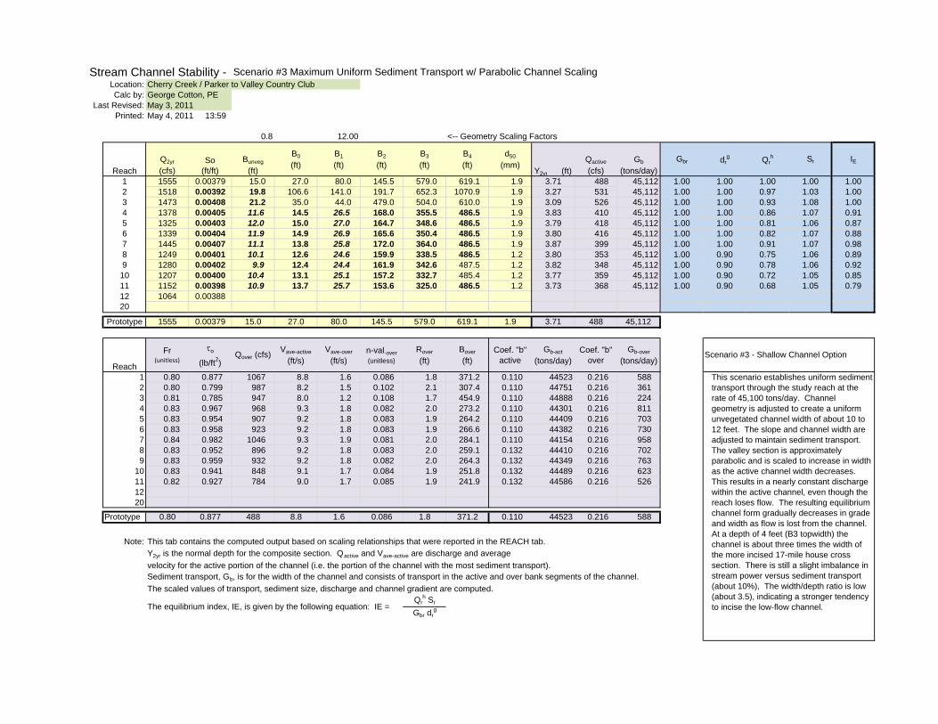
Stream Channel Stability - Scenario #3 Maximum Uniform Sediment Transport w/ Parabolic Channel ScalingLocation:Calc by:
Last Revised:Printed:
0.8 12.00 <-- Geometry Scaling Factors
ReachQ2yr
(cfs)So
(ft/ft)Bunveg
(ft)
B0
(ft)B1
(ft)B2
(ft)B3
(ft)B4
(ft)d50
(mm)Y2yr (ft)
Qactive
(cfs)Gb
(tons/day)Gbr dr
g Qrh Sr IE
1 1555 0.00379 15.0 27.0 80.0 145.5 579.0 619.1 1.9 3.71 488 45,112 1.00 1.00 1.00 1.00 1.002 1518 0.00392 19.8 106.6 141.0 191.7 652.3 1070.9 1.9 3.27 531 45,112 1.00 1.00 0.97 1.03 1.003 1473 0.00408 21.2 35.0 44.0 479.0 504.0 610.0 1.9 3.09 526 45,112 1.00 1.00 0.93 1.08 1.004 1378 0.00405 11.6 14.5 26.5 168.0 355.5 486.5 1.9 3.83 410 45,112 1.00 1.00 0.86 1.07 0.915 1325 0.00403 12.0 15.0 27.0 164.7 348.6 486.5 1.9 3.79 418 45,112 1.00 1.00 0.81 1.06 0.876 1339 0.00404 11.9 14.9 26.9 165.6 350.4 486.5 1.9 3.80 416 45,112 1.00 1.00 0.82 1.07 0.887 1445 0.00407 11.1 13.8 25.8 172.0 364.0 486.5 1.9 3.87 399 45,112 1.00 1.00 0.91 1.07 0.988 1249 0.00401 10.1 12.6 24.6 159.9 338.5 486.5 1.2 3.80 353 45,112 1.00 0.90 0.75 1.06 0.899 1280 0.00402 9.9 12.4 24.4 161.9 342.6 487.5 1.2 3.82 348 45,112 1.00 0.90 0.78 1.06 0.92
10 1207 0.00400 10.4 13.1 25.1 157.2 332.7 485.4 1.2 3.77 359 45,112 1.00 0.90 0.72 1.05 0.8511 1152 0.00398 10.9 13.7 25.7 153.6 325.0 486.5 1.2 3.73 368 45,112 1.00 0.90 0.68 1.05 0.7912 1064 0.0038820
Prototype 1555 0.00379 15.0 27.0 80.0 145.5 579.0 619.1 1.9 3.71 488 45,112
Reach
Fr (unitless)
τo (lb/ft2)
Qover (cfs) Vave-active
(ft/s)Vave-over
(ft/s)n-val-over (unitless)
Rover
(ft)Bover
(ft)Coef. "b"
activeGb-act
(tons/day)Coef. "b"
overGb-over
(tons/day)
1 0.80 0.877 1067 8.8 1.6 0.086 1.8 371.2 0.110 44523 0.216 5882 0.80 0.799 987 8.2 1.5 0.102 2.1 307.4 0.110 44751 0.216 3613 0.81 0.785 947 8.0 1.2 0.108 1.7 454.9 0.110 44888 0.216 2244 0.83 0.967 968 9.3 1.8 0.082 2.0 273.2 0.110 44301 0.216 8115 0.83 0.954 907 9.2 1.8 0.083 1.9 264.2 0.110 44409 0.216 7036 0.83 0.958 923 9.2 1.8 0.083 1.9 266.6 0.110 44382 0.216 7307 0.84 0.982 1046 9.3 1.9 0.081 2.0 284.1 0.110 44154 0.216 9588 0.83 0.952 896 9.2 1.8 0.083 2.0 259.1 0.132 44410 0.216 7029 0.83 0.959 932 9.2 1.8 0.082 2.0 264.3 0.132 44349 0.216 763
10 0.83 0.941 848 9.1 1.7 0.084 1.9 251.8 0.132 44489 0.216 62311 0.82 0.927 784 9.0 1.7 0.085 1.9 241.9 0.132 44586 0.216 5261220
Prototype 0.80 0.877 488 8.8 1.6 0.086 1.8 371.2 0.110 44523 0.216 588
Note: This tab contains the computed output based on scaling relationships that were reported in the REACH tab. Y2yr is the normal depth for the composite section. Qactive and Vave-active are discharge and average velocity for the active portion of the channel (i.e. the portion of the channel with the most sediment transport).Sediment transport, Gb, is for the width of the channel and consists of transport in the active and over bank segments of the channel. The scaled values of transport, sediment size, discharge and channel gradient are computed.
Qrh Sr
Gbr drg
Scenario #3 - Shallow Channel Option
This scenario establishes uniform sediment transport through the study reach at the rate of 45,100 tons/day. Channel geometry is adjusted to create a uniform unvegetated channel width of about 10 to 12 feet. The slope and channel width are adjusted to maintain sediment transport. The valley section is approximately parabolic and is scaled to increase in width as the active channel width decreases. This results in a nearly constant discharge within the active channel, even though the reach loses flow. The resulting equilibrium channel form gradually decreases in grade and width as flow is lost from the channel. At a depth of 4 feet (B3 topwidth) the channel is about three times the width of the more incised 17-mile house cross section. There is still a slight imbalance in stream power versus sediment transport (about 10%), The width/depth ratio is low (about 3.5), indicating a stronger tendency to incise the low-flow channel.The equilibrium index, IE, is given by the following equation: IE =
Cherry Creek / Parker to Valley Country ClubGeorge Cotton, PEMay 3, 2011May 4, 2011 13:59

GEORGE K COTTON CONSULTING, INC
HYDROLOGIC ENGINEERING AND DESIGN
SCENARIO DEVELOPMENT AND EVALUATION 23 | P A G E
APPENDIX B. STABILITY INDEX METHOD
Equilibrium relationships are commonly used in the assessment of stream stability. They have their origins in empirical (Leopold and Maddock, 1953) and qualitative relationships of river process (Lane, 1955). It can be shown that scaling of steady, uniform turbulent flow in a non-prismatic channel with an alluvial boundary provides the basis for these relationships. As a result, an upstream channel section that is in equilibrium can be used to scale downstream channel sections in accordance with the yield of water and sediment.
GRADUALLY VARIED FLOW
The differential equation for one-dimensional gradually varied open-channel flow (Henderson, 1966 see Equation 4-31) can be written as:
dDdx ( )1 - αFr2 = S - Sf ............................................................................. (1)
where x is the distance in the downstream direction, D is the flow depth, α is the energy coefficient (assumed constant),
Fr is the Froude number (Fr2 = V2
gD ),
V is the average velocity, g is the acceleration of gravity, and S, Sf are the channel gradient and friction slope, respectively.
PROTOTYPE/MODEL SIMILITUDE
The scaling of hydraulic geometry can be explored using similitude methods (Griffiths, 2003). Assuming that the at-station situation is the prototype, equation 1 can be written as:
dDpdxp
( )1 - αFrp2 = Sp - Sfp ....................................................................... (2)
The subscript p denotes the prototype version.
The downstream situation is the model version of equation 1:
dDmdxm
( )1 - αFrm2 = Sm - Sfm .................................................................... (3)
The subscript m denotes the model version.
Substitution of Dm = Dr Dp and similarly for other variables in equation 3 yields:
1Sp
dDpdxp
⎝⎜⎛
⎠⎟⎞Dr
Sr xr ( )1 - α Fr2
p ( )Fr2r = 1 -
Sfp Sp
⎝⎜⎛
⎠⎟⎞Sfr
Sr .................................. (4)
The subscript r denotes the ration of model to prototype (i.e. a dimensionless variable).

GEORGE K COTTON CONSULTING, INC
HYDROLOGIC ENGINEERING AND DESIGN
SCENARIO DEVELOPMENT AND EVALUATION 24 | P A G E
For dynamic similarity to hold at model and prototype sections equations 2 and 4 must be identical, which implies from equation 4 that:
DrSr xr
= 1 .................................................................................................. (5a)
SfrSr
= 1 .................................................................................................... (5b)
Frr2
= 1 .................................................................................................. (5c)
From the equation of continuity we have the following scaling relationship.
Qr = Vr Br Dr ........................................................................................... (6)
where: Br is the dimensionless channel width, Qr is the dimensionless discharge, Vr is the dimensionless velocity, and xr is the dimensionless reach length.
EFFECT OF ROUGHNESS
Using the Manning formula for fully rough flow the friction slope is:
Sf = g ⎝⎜⎛
⎠⎟⎞n2
D1/3 Fr2 ...................................................................................... (7)
where g is the acceleration of gravity and n is the Manning roughness coefficient.
In scaling terms equation 7 can be written as:
Sfr = ⎝⎜⎜⎛
⎠⎟⎟⎞nr
2
Dr 1/3 Frr
2 ................................................................................... (8)
From the Strickler equation (Henderson, 1966 see Equation 4-23) the roughness scaling is a function of a characteristic sediment grain size, d.
nr = dr1/6 .................................................................................................. (9)
where: dr is the dimensionless particle size.
Equation 8 can then be rewritten as:
Sfr = ⎝⎜⎛
⎠⎟⎞ dr
Dr
1/3
Frr2 ................................................................................. (10)

GEORGE K COTTON CONSULTING, INC
HYDROLOGIC ENGINEERING AND DESIGN
SCENARIO DEVELOPMENT AND EVALUATION 25 | P A G E
SCALING OF SEDIMENT TRANSPORT
Stream form is also dependent on the transport of bed load either in contact with the bed or in suspension. In natural streams where the supply of sediment is not interrupted by excessive deposition or scour (such is caused by a dam), this exchange of bed material maintains a gradation of sediment sizes. Power function versions of sediment transport have been developed for rivers of various sizes and alluvial material. Transport functions may also be derived from sediment transport calculations.
A general power function for unit rate of sediment transport is:
gb = b' Vm1
Dm2
...................................................................................... (11)
where: b’, m1, m2 are coefficients of the power function.
The total bed-load sediment transport in a channel is:
Gb = B gb ............................................................................................... (12)
where: B is the width of the active channel.
The dimensionless form of equation 12 is:
Gbr = Br Vrm1
Drm2
.................................................................................. (13)
ALLUVIAL CHANNEL SCALING RELATIONSHIPS
Adopting the active channel width, B, as the longitudinal scale (Br = xr), equation 5 gives the following scaling relationships.
Sfr = DrBr
= ⎝⎜⎛
⎠⎟⎞ dr
Dr
1/3
Vr
2
Dr ....................................................................... (14a)
Br = Dr
4/3
dr1/3 ............................................................................................ (14b)
Substituting 14b and 5c into 6 gives:
Qr = ⎝⎜⎜⎛
⎠⎟⎟⎞Dr
4/3
dr1/3 Dr
1/2 Dr ............................................................................ (15a)
Dr = Qr6/17 dr
2/17 ................................................................................. (15b)
Substituting 15b back into 14b gives:
Br = Qr8/17 dr
-3/17 ................................................................................... (16)
Substituting 15b into 5c gives:

GEORGE K COTTON CONSULTING, INC
HYDROLOGIC ENGINEERING AND DESIGN
SCENARIO DEVELOPMENT AND EVALUATION 26 | P A G E
Vr = Dr1/2 ............................................................................................ (17a)
Vr = Qr3/17 dr
1/17 ................................................................................. (17b)
Substituting 15b and 16 into 5a gives:
Sr = DrBr
................................................................................................ (18a)
Sr = Qr-2/17 dr
5/17 ................................................................................ (18b)
Substituting 15b, 16 and 17b into 13 gives:
Gbr = Qre dr
f .......................................................................................... (19)
where: e = (8 + 3m1 +6m2)/17; f = (-3 + m1 + 2m2)/17
Summarizing, the theoretically derived scaling relationships for channel geometry are as follows.
Dr = Qr6/17 dr
2/17 ................................................................................... (15)
Br = Qr8/17 dr
-3/17 ................................................................................... (16)
Vr = Qr3/17 dr
1/17 ................................................................................... (17)
Sr = Qr-2/17 dr
5/17 .................................................................................. (18)
Gbr = Qre dr
f .......................................................................................... (19)
The exponents of Q from the theoretically derived scaling relations are very similar to those from the
empirical results of Leopold and Maddock (1953) as summarized in Table 1. The introduction of sediment size, d, by the theoretical derivation gives insight into processes related to channel roughness.
Table 8. Comparison of Empirical and Theoretical Scaling Exponents
Scaling Empirical* Theoretical Variable j j’ k’
Br 0.5 0.47 -0.18
Dr 0.4 0.35 0.12
Vr 0.1 0.18 0.06
Sr -0.1 -0.12 0.29
Gbr none Function of sediment transport relationship
*Leopold and Maddock (1953)

GEORGE K COTTON CONSULTING, INC
HYDROLOGIC ENGINEERING AND DESIGN
SCENARIO DEVELOPMENT AND EVALUATION 27 | P A G E
STABLE CHANNEL ASSESSMENT – EQUILIBRIUM RELATIONSHIPS
LANE RELATIONSHIP - ENHANCED
Lane (1955) describes a general equilibrium relationship among river hydraulic variables, which is often used as the basis for qualitative geomorphic analysis.
Gb d α Q S ........................................................................................ (20)
The relationship is applied by assuming that two of the variables remain constant. For example, an increase in bed load +Gb, with no change in sediment size d, or stream discharge Q, will result in an increase in stream slope +S. This is interpreted as a potential for sediment deposition in the existing stream channel. A similar relationship can be derived by dividing equation 18 by equation 19.
Gbr drg = Qr
h Sr .................................................................................. (21)
where: g = 5/17 – f; and, h = 2/17 + e The theoretically derived equilibrium relationship offers insights into the interplay of alluvial variables
that is missing from applying equations 15-19 individually. First, the strong relationship between stream discharge, gradient, and sediment transport is clearly evident. The role of sediment size appears modest, although sediment size can adjust several orders of magnitude due to armoring. The derived equilibrium relationship (21) offers a clear conceptual framework for quantitative analysis. The scaling relationships, which are at-station (prototype) to downstream-station (model), offer a spatial context.
EQUILIBRIUM INDEX APPROACH
Alternatively, the scaling relationships can be formulated as an index, where the index is determined from the properties of the stable prototype cross section relative to other cross sections. The stability index for the prototype reach is 1.0. If other cross sections are also in equilibrium their stability index will also be near 1.0. Index values that are not unity indicate non-equilibrium downstream conditions. Values of IE can then be applied to assessing other downstream cross sections.
Equation 21 can be stated as the following equilibrium index:
IE = Qr
h Sr
Gbr drg ........................................................................................ (22)