chemical reaction engineering - nptel.ac.in · non-isothermal reactors - cstr 0.0 0.2 0.4 0.6 0.8...
TRANSCRIPT

Chemical Reaction Engineering Reactor Design
Jayant M. Modak Department of Chemical Engineering Indian Institute of Science, Bangalore
Chemical Reactor Design
Ø Objectives q Technological
n Maximum possible product in minimum time n Desired quantity in minimum time n Maximum possible product in desired time
q Economic n Maximize profit
Chemical Reactor Design
Ø Constraints q Market
n Raw materials availability – quality and quantity n Demand for the product
q Society/Legislative n Safety n Pollution control
q Technological n Thermodynamics n Stoichiometry n Kinetics

Chemical Reactor Design - Decisions
Ø Type of reactor q Tubular, Fixed Bed, Stirred tank, Fluidized bed
Ø Mode q Mass Flow: Batch, Continuous, Semibatch q Energy: Isothermal, Adiabatic, Co/counter current
Ø Process Intensification q Combining more than one type of unit operation

Tubular reactor – mass balance
Indian Institute of Science
( ) ( )
( ) 0
j jj j j j j
j j j j j j j jj j j j
ff
C CFlux R uC J R
t z t z
M C u M C M J M Rt z
ut xρ
ρ
∂ ∂∂ ∂+ = + + =∂ ∂ ∂ ∂
⎛ ⎞ ⎛ ⎞∂ ∂+ + =⎜ ⎟ ⎜ ⎟∂ ∂⎝ ⎠ ⎝ ⎠
∂ ∂+ =∂ ∂
∑ ∑ ∑ ∑

Tubular reactor – energy balance
Indian Institute of Science
( )
( ) ( )
( )
1
j
j
T T j jj
T T
T
j
jj
j
jj
j
j Pj
j Pj
jj
jj
jj
j
j
C U F H A H J Qt A z
C U C H Pt t
F
TC Ct
TF C
CH
t
FH
z
JH
z
H
Hz
H Jz z
Jz
∂⎛ ⎛ ⎞ ∂⎜ ⎟ ∂⎝
⎞
⎛ ⎞∂ ∂+ + =⎜ ⎟∂ ∂ ⎝ ⎠∂ ∂= − = +∂ ∂
∂ = +∂
⎛ ⎞∂ = +⎜ ⎟∂ ⎝
⎠⎛ ⎞ ∂⎜ ⎟ ∂⎝ ⎠
∂
⎜ ⎟ ∂⎝ ⎠∂⎛ ⎞
⎜ ⎟ ∂⎝ ⎠∂⎛ ⎞
⎜ ⎟ ∂⎝ ⎠
⎞∂⎠⎠
⎛⎜ ⎟⎝
∑
∑
∑∑
∑
∑
∑
∑

Tubular reactor – energy balance
Indian Institute of Science
( )
( )
4
1
4
j
j
j j jj j j i i
j j
j P
rt
r
i
ij
ii t
j
j P
Q U
C F JH A H R H r
t A z z
T TC C
H
T Td
U T T
ut u
T TC C uu d
rt
⎛ ⎞ ∂ ∂⎛ ⎞+⎜ ⎟⎜ ⎟∂ ∂⎝ ⎠⎝ ⎠
∂ ∂ ∂⎛ ⎞ ⎛ ⎞⎛ ⎞⎡ ⎤+ + = Δ⎜ ⎟ ⎜ ⎟⎜ ⎟⎢ ⎥∂ ∂ ∂⎣
⎛ ⎞ ∂ ∂⎛ ⎞+ +⎜ ⎟⎜ ⎟∂ ∂⎝ ⎠
⎦⎝ ⎠=
= −
−⎝
⎝ ⎠
⎠
⎝ ⎠
Δ =
∑ ∑ ∑
∑
∑
∑

Stirred tank reactor – mass and energy balance
Indian Institute of Science
( ) ( ) ( )
0
0 0j
jj je j
j P i ii
Kj j jej j
rdTN C F H Hdt
V
dNF F R
dt
A U Tr TH= −⎛ ⎞
− +⎜ ⎟
=
Δ⎠
+
+
−⎝
−
∑∑ ∑

Fixed bed reactor – mass balance
( ) ( )
( )
( )
( )( )
,
,
2
2
,
4
,1 ( , ),
j
B j B j mj
jB j s j ej s f mj
f
rt
e
j P s ej
j
e
h
r j
r
C Flux qt z
CC u C D q
t z z
U T Td
D CYrX X
qT T TC C ut z
Yr
z
r T
ε ε
ε ρρ
λ
λ⎛
∂ ∂+ =∂ ∂
⎛ ⎞⎛ ⎞∂ ∂ ∂+ − =⎜ ⎟⎜ ⎟⎜ ⎟⎜ ⎟∂ ∂ ∂ ⎝ ⎠⎝ ⎠
−
∂ ∂⎛ ⎞ =⎜ ⎟∂
⎞⎛ ⎞∂ ∂ ∂+ − +⎜ ⎟⎜ ⎟∂ ∂ ∂⎝ ⎠⎝=
∂⎝ ⎠
⎠∑

Psuedohomogenous model
Indian Institute of Science
mj
h ii
j
i
q R
q H r
=
= Δ∑

Heterogenous model – external diffusion
Indian Institute of Science
( )
( )( )
( )
( ) ( )
3 1
( ) ,
mj g j js p g v j js
v B
h f v s
g v j js j js s
f i ii
v s
q K C C n A K a C C
aR
q h a T T
K a C C R C T
h a HT T r
ε
= − − = − −
= −
= −
− =
Δ
−
− =∑
g g

Heterogenous model – internal diffusion
Indian Institute of Science
( )
( )
( )
'
'2 ' ' ' '
2
'2 '
2
''
1 ,
1i
j
ej j
ii
i i ii
j
e
jmj ej v j j
r R
h
Cr D R C T
r r r
Tr H r
H r
r r r
Cq D a R C
r
q
η
η
λ
=
⎛ ⎞∂∂ = −⎜ ⎟⎜ ⎟∂ ∂⎝ ⎠⎛ ⎞∂∂ =⎜ ⎟⎜ ⎟∂ ∂⎝ ⎠
∂= −
−Δ
=∂
=
Δ∑
∑

Non-isothermal reactors - PFR
0.0 0.5 1.0 1.5 2.0 2.5 3.0 3.5 4.00
1
2
300
325
3500 10 20 30 40
0.00.51.01.52.0
Concentration temperature
Time (min)
Adiabatic Isothermal
Con
cent
ratio
n
Indian Institute of Science

Non-isothermal reactors - CSTR
0.0 0.2 0.4 0.6 0.8 1.0 1.2 1.4 1.6 1.8 2.00.0
0.5
1.0
1.5
2.0300
320
340C
once
ntra
tion
Residence time
Tem
pera
ture

Non-isothermal reactors - rate
Indian Institute of Science
0.0 0.5 1.0 1.5 2.00
2
4
6
8 r11/rate
C10-C1

Trajectories - Exothermic reaction
Indian Institute of Science
300 320 340 360 380 4000.0
0.2
0.4
0.6
0.8
1.0 X
eq
T
Isothermal
Adiabatic

Trajectories - Endothermic reaction
Indian Institute of Science
300 320 340 360 380 4000.0
0.2
0.4
0.6
0.8
1.0
Xeq
T
Isothermal
Adiabatic

Optimal temperature trajectories
0.0 0.2 0.4 0.6 0.8 1.00.01
0.1
1
10
100
1/ra
te
conversion
0.0 0.2 0.4 0.6 0.8 1.00.01
0.1
1
10
Rate
conversion
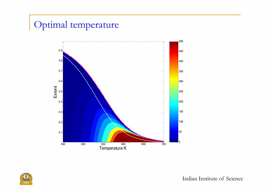
Optimal temperature
Indian Institute of Science
0
50
100
150
200
250
300
350
400
450
500
450 500 550 600 650 700
0.1
0.2
0.3
0.4
0.5
0.6
0.7
0.8
0.9
Temperature K
Exte
nt

Thermal cracking of ethane in tubular reactor
Ø Ethylene demands – polyethylene, ethylene oxide, ethylene glycol – 20 million tons per annum
Ø Main Reaction increase in number of moles so steam as inert
Ø Endothermic reaction - ∆H 34.5 kcal/mol, high
temperature for high equilibrium conversions, increasing temperatures along the length of the reactor
Ø Side reactions higher conversion yield of side products higher
Indian Institute of Science
2 6 2 4 2C H C H H→ +
2 6 3 8 42C H C H CH→ +

Indian Institute of Science
Yield conversion diagram for ethane cracking

Ethane cracking reactor
Indian Institute of Science
Typical operating condn
• L = 95 m
• G = 68.68 kg/m2/s
• P inlet 2.99 atm, outlet 1.2 atm
• T inlet 680, outlet 820 C
• Production 10000 tons/coil

Balances
( )
2
2
2
41 ( )
4
2
' 1
t
t
jj
t i iij pj
j
f ft b i
jj
ddFmass R
dzddTenergy q z d H r
dz F C
dp f dumomentum u udz d r dz
RT FFuA A p
π
ππ
ξ ρ ρπ
=
⎡ ⎤= + − Δ⎢ ⎥
⎣ ⎦
⎡ ⎤− = + +⎢ ⎥
⎣ ⎦⎡ ⎤⎢ ⎥= = ⎢ ⎥⎢ ⎥⎣ ⎦
∑∑
∑
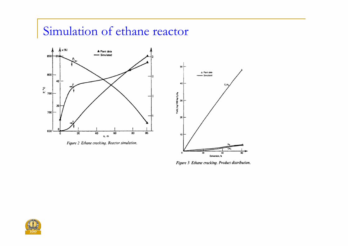
Simulation of ethane reactor

Hydrogenation of oil
Ø Major demand – margarine, shortenings, vanaspati
Ø Vegetable oils – mixture of triglycerides - glycerol and fatty acids
Ø Fatty acids – saturated (S) , monosaturated (cis, R1 and trans, R2) and diunsaturated (B). Hydrogenation to reduce odor or color, improve stability and increase melting point.
Ø Product requirements – some polyunsaturated
(health) and R2 ( consistency and higher melting points)

Reactions
2 2
1/ 21 4 5 6,H Hr r C r r C− ∝ − ∝
implies selectivity of monounsaturates over saturates proportional to (CH2)1/2
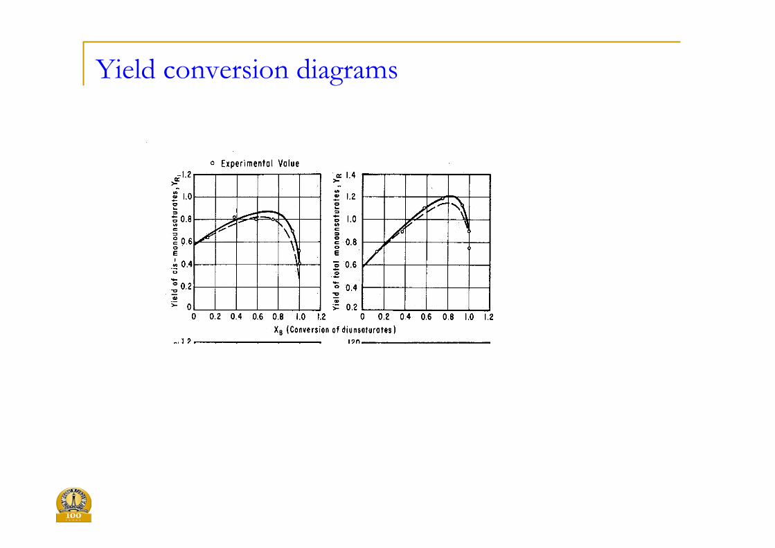
Yield conversion diagrams

Balances
( ) ( )( ) ( )
( )
2 2 2 2
2
2 2 2 2
2 2 2
1 2
, , ,
,, , , ,
, ,
, , ,
,
0
1 1 1
jj
L v H g H s H j H s
H bL v H g H b S S H b H s
S S H b H s H
L v S SL v
dCmass R j B R R M
dtk a C C R C C
dCk a C C k a C C
dtk a C C R
k a k ak a
= =
− − =
= − − −
= − +
= +
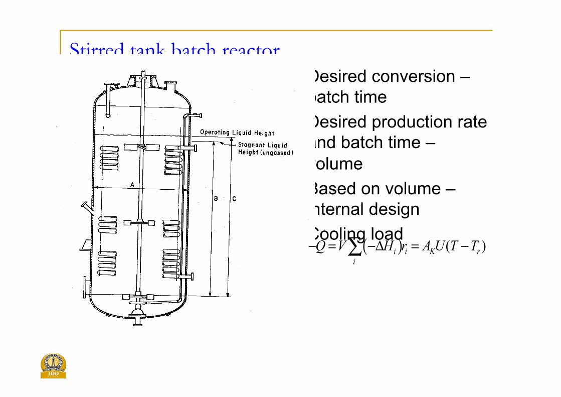
Stirred tank batch reactor Ø Desired conversion –
batch time Ø Desired production rate
and batch time – volume
Ø Based on volume – internal design
Ø Cooling load ( ) ( )i i K ri
Q V H r A U T T− = −Δ = −∑
Ammonia synthesis
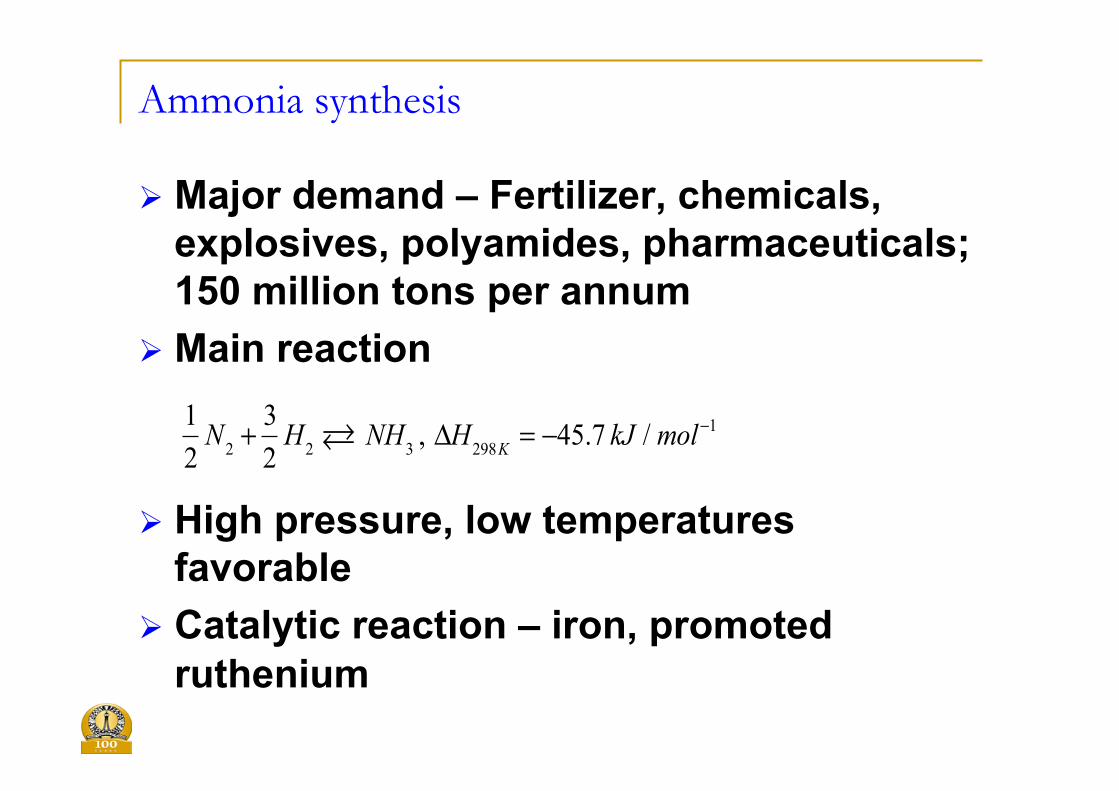
Ø Major demand – Fertilizer, chemicals, explosives, polyamides, pharmaceuticals; 150 million tons per annum
Ø Main reaction Ø High pressure, low temperatures
favorable Ø Catalytic reaction – iron, promoted
ruthenium
12
N2 +32
H2 ! NH3 , !H298K = "45.7 kJ / mol"1

Ammonia synthesis – equilibrium
Indian Institute of Science
500 600 700 800 9000.00.10.20.30.40.50.60.70.80.91.0
(A)
1
310
50
100
200
P = 300 atm
A
mm
onia
Mol
frac
tion
Temperature (K)0 100 200 300
0.00.10.20.30.40.50.60.70.80.91.0
(B)
773
723
673
623
573
523
T = 473 K
Am
mon
ia M
ol fr
actio
nPressure (Atm)

Ammonia synthesis - balances
Indian Institute of Science
( )
( ) ( )
( )'
2 ' '2
'2
2
,
4
1 ,
1
js j j
f s p rt
iie i i
e
dCmass u R C T
dzdT Uenergy u c T T H rdz d
dCd r D R C Tr dr dr
catalystdTd r H r
r dr dr
η
ρ η
λ
=
= − + −Δ
⎛ ⎞= −⎜ ⎟
⎝ ⎠⎛ ⎞
= Δ⎜ ⎟⎝ ⎠

Reactor simulation
0 1 2 3 4 50
20
40
60
80
100
120
rate at bulk conditions observed rate
rate
Length (m)
Indian Institute of Science
0 1 2 3 4 50.0
0.1
0.2
0.3
0.4
0.5
0.6
0.7
N2
H2
NH3
m
ol fr
actio
n
Length (m)0 1 2 3 4 5
680700720740760780800820840860
tem
pera
ture
Length (m)

Optimal temperature
Indian Institute of Science
0
50
100
150
200
250
300
350
400
450
500
450 500 550 600 650 700
0.1
0.2
0.3
0.4
0.5
0.6
0.7
0.8
0.9
Temperature K
Exte
nt

Fixed bed reactors
Indian Institute of Science
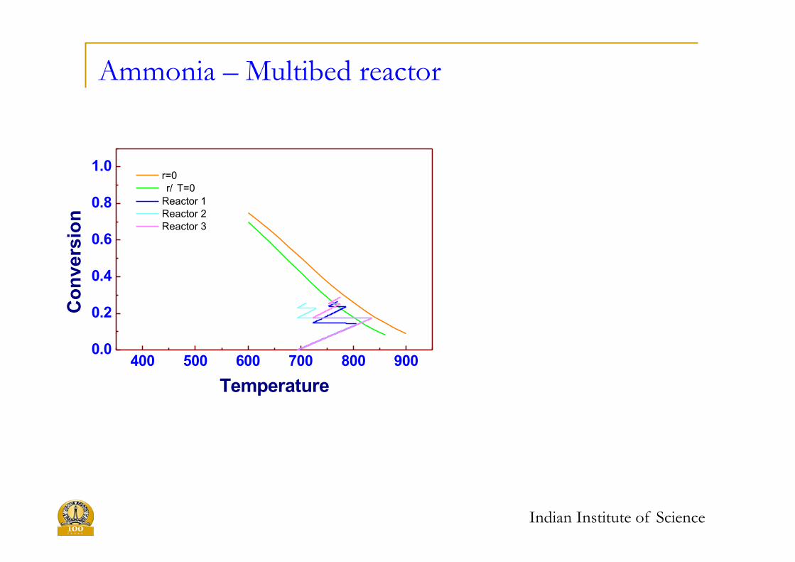
Ammonia – Multibed reactor
400 500 600 700 800 9000.0
0.2
0.4
0.6
0.8
1.0 r=0 r/ T=0 Reactor 1 Reactor 2 Reactor 3
Conversion
Temperature
Indian Institute of Science

Fixed bed reactors
Indian Institute of Science

Ammonia – Autothermal
400 500 600 700 800 900 10000
50
100
150
200
250
300 Ttop-T1L
Ttop-Tfeed
473 491 513 523 578 623
ΔΤ
Ttop
Indian Institute of Science
400 500 600 700 800 900 1000400
500
600
700
800
900
1000
T feed
K
Ttop K

Ammonia – Autothermal
0 1 2 3 4 5 6
500
550
600
650
700
750
800
reactor heat exchanger
Conversion
Length
Indian Institute of Science
600 650 700 750 800 850 9000.00.10.20.30.40.50.60.70.8
r=0 ∂r/∂T=0
Conversion
Temperature

Process intensification
Ø Strategy of reduction in physical size of a chemical plant while achieving given objective
Ø 30 – 40 years old concept, reinvented in last decade due to intense competition, scarce resources and stricter environmental norms
Ø Multifunctional reactive systems – several functions are designed to occur simultaneously.
Ø Major drive in refining and petrochemicals sector
Indian Institute of Science

Catalyst particle in reacting media
Ø Type A – at catalyst level Ø Type B – at interphase
transport level Ø Type C – at intra-reactor
level – separations/heat transfer
Ø Type D – inter-reactor level by combining two reactor operation with solids recirculation.
Indian Institute of Science
Type A Example – bifunctional catalysis
Ø Catalytic reforming to increase the octane number
Ø Conversion of parafins, cyclo parafins and napthenes to aromatics and branced paraffins.
Ø Reactions involved – dehydrogenation, cyclization and isomerization
Ø Pt/SiO2 catalyst
Indian Institute of Science

Type B Example – Gas induction reactors
Indian Institute of Science
DISPERSIONGAS-LIQUID
STATORDRAFT TUBE
DISPERSING IMPELLER
SUSPENDING IMPELLER
SELF INDUCING IMPELLER
GAS ENTRANCE
DISPERSIONGAS-LIQUID
STATORDRAFT TUBE
DISPERSING IMPELLER
SUSPENDING IMPELLER
SELF INDUCING IMPELLER
GAS-LIQUID
STATORDRAFT TUBE
DISPERSING IMPELLER
SUSPENDING IMPELLER
SELF INDUCING IMPELLER
GAS ENTRANCE
GAS - LIQUID DISPERSION
STATOR DRAFT TUBE

Type C – Intra-reactor operation
Ø Energy transfer – reaction in heat exchanger Ø Momentum transfer – radial flow reactors Ø Mass transfer – reactive- distillation,
absorption
Indian Institute of Science

Type C – Momentum transfer
Ø High gas flow rates – ammonia synthesis, styrene from ethylbenzene, flue gas treatments
Indian Institute of Science

Type C – Mass transfer
Ø Enhance conversion in equilibrium limited reaction, prevent undesirable reaction, increase rate of product inhibited reactions
Indian Institute of Science

Type C – Energy transfer
0 1 2 3 4 5 60.00
0.05
0.10
0.15
0.20
0.25
0.30
Flue gas Process
Temperature
Length
Indian Institute of Science
4 2 2
4 2 2 2
3 206 /2 2 803 /
CH H O CO H H kJ molCH O CO H O H kJ mol
+ + Δ =+ + Δ = −
ÉÉ
0 1 2 3 4 5 6
640
680
720
760
800
840
Flue gas Process
Temperature
Length

Type C – Example styrene synthesis
Indian Institute of Science

Design considerations and safety
Indian Institute of Science

Multiplicity in stirred tank reactor
Indian Institute of Science

Explosion in batch reactor
Indian Institute of Science

Runaway/Hot spot in tubular reactor
Indian Institute of Science
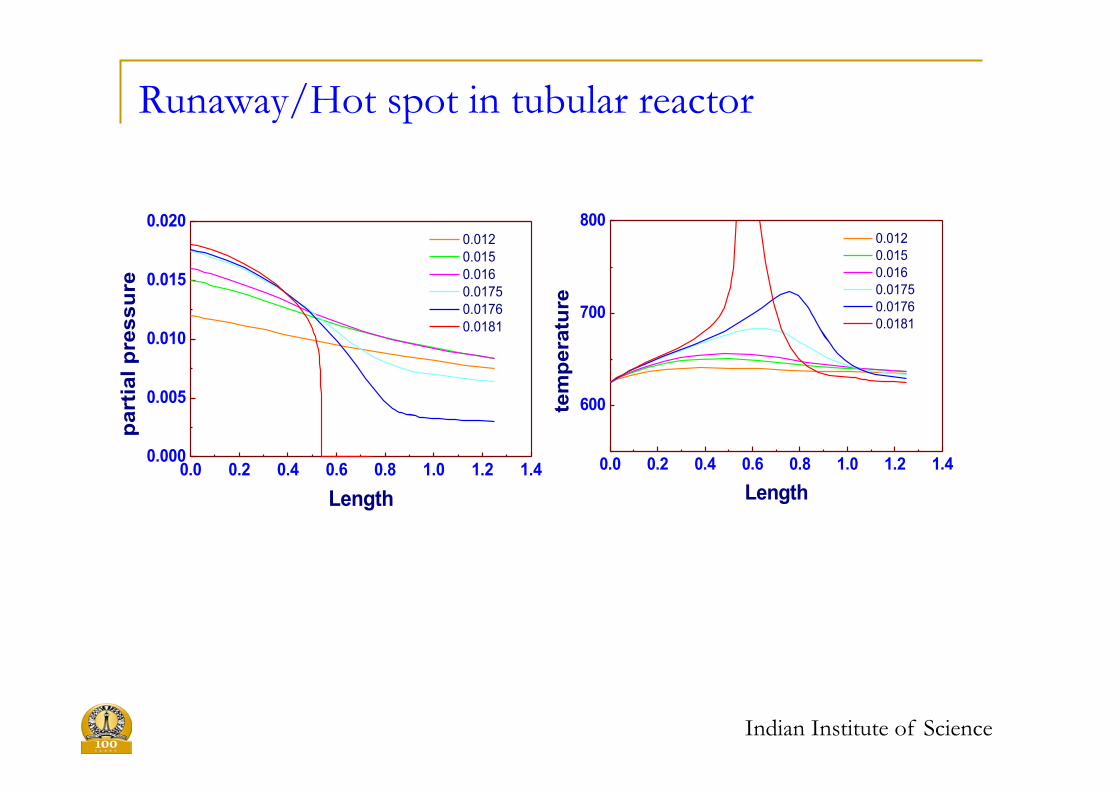
Runaway/Hot spot in tubular reactor
Indian Institute of Science
0.0 0.2 0.4 0.6 0.8 1.0 1.2 1.40.000
0.005
0.010
0.015
0.020
0.012 0.015 0.016 0.0175 0.0176 0.0181
part
ial p
ress
ure
Length0.0 0.2 0.4 0.6 0.8 1.0 1.2 1.4
600
700
800
0.012 0.015 0.016 0.0175 0.0176 0.0181
temperature
Length

Runaway/Hotspot in tubular reactors
Indian Institute of Science
610 620 630 640 650 660
0.004
0.008
0.012
0.016
0.020
Par
tial p
ress
ure
temperature
Sensitive
Insensitive

Indian Institute of Science
q=det (A)
>= ±
>
q p
iλ α βα
2
1,2
/ 4
0
=q p2 / 4
>= ±
>
q p
iλ α βα
2
1,2
/ 4
0
>= ±
<
q p
iλ α βα
2
1,2
/ 4
0
<=<
q p
λ α αα
2
1,2 1 2
/ 4
,
' ' 0
<=<
q p
λ α αα
2
1,2 1 2
/ 4
,
' ' 0
<=
> >
q p
λ α αα α α
2
1,2 1 2
1 1 2
/ 4
,
0,
<= >
q p
λ α α
2
1,2 1 2
/ 4
, 0
p=tr (A)

Stability analysis
Ø A state X=0 is said to be stable when given e>0, there exists a d>0 (0<d<e) such that if ||X(0)||<d then ||X(t)|| < e for all t>0
Ø A state X=0 is said to be asymptotically attractive when given m>0, such that if ||X(0)||<m then lim (t→∞) ||X(t)|| =0
Ø A state is asymptotically stable when stable and asymptotically attractive.
Ø A state is marginally stable when stable but not asymptotically attractive
Indian Institute of Science

Examples
Indian Institute of Science
( )( )
( )( )
2 5
22 2 2 2
2
22 2 2 2
1
2
1
x y x ydxdt x y x y
y y xdydt x y x y
− +=
+ + + +
−=
+ + + +
0.0 0.2 0.4 0.6 0.8 1.00.0
0.2
0.4
0.6
0.8
1.0
Y
X
dx ydtdy xdt
=
= −
-1.2-1.0-0.8-0.6-0.4-0.2 0.0 0.2 0.4 0.6 0.8 1.0 1.2-1.2-1.0-0.8-0.6-0.4-0.20.00.20.40.60.81.01.2
Y
X

Two dimensional system - Eigen values
Indian Institute of Science
22
1,202 4T TT D Dλ λ λ− + = ⇒ = ± −
0
Stablenode
Stablefocus
Unstablefocus
D=determinant(A)
T=trace(A)
T2/4-D=0
Unstablenode

Unstable node
Indian Institute of Science
0.1 0.00971, 0.988 0.0099,0.9782D Tµ λ= = = =
-50 0 50 100 150 200 250 300 35010
15
20
25
30
35
40
45
-50 0 50 100 150 200 250 300 350
0.00
0.02
0.04
0.06
0.08
0.10
10 20 30 40 50
0.00
0.02
0.04
0.06
0.08
0.10
alpha
Time
beta
Time
beta
alpha
0
Stablenode
Stablefocus
Unstablefocus
D=determinant(A)
T=trace(A)
T2/4-D=0
Unstablenode

Unstable focus
Indian Institute of Science
0.5 0.248, 0.751 0.3756 0.3276iD Tµ λ= = = = ±
-50 0 50100150200250300350400450500550600650700750-50
0
50
100
150
200
250
300
350
-50 0 50 100 150 200 250 300 3500.0
0.5
1.0
1.5
2.0
2.5
3.0
-10 0 10 20 30
0.0
0.5
1.0
1.5
2.0
2.5
3.0
0 2 4 6 8 10 12 14 16 18 20-10-8-6-4-20246810
alpha
Time
beta
Time
beta
alpha
linearized process real process
beta
alpha
0
Stablenode
Stablefocus
Unstablefocus
D=determinant(A)
T=trace(A)
T2/4-D=0
Unstablenode

Stable focus
-50 0 50 100 150 200 250 300 3500.45
0.50
0.55
0.60
0.65
0.70
0.75
0.80
-50 0 50 100 150 200 250 300 3501.4
1.5
1.6
1.7
1.8
1.9
2.0
2.1
0.45 0.50 0.55 0.60 0.65 0.70 0.75 0.801.4
1.5
1.6
1.7
1.8
1.9
2.0
2.1
-2 0 2 4 6 8 10
0.0
0.1
0.2
0.3
alph
a
Time
beta
Time
beta
alpha
Δ a
lpha
alpha
Indian Institute of Science
2.0 3.99, 2.98 -1.4900 1.3288iD Tµ λ= = = − = ± 0
Stablenode
Stablefocus
Unstablefocus
D=determinant(A)
T=trace(A)
T2/4-D=0
Unstablenode

Stable node
-50 0 50 100 150 200 250 300 350
0.40
0.45
0.50
0.55
0.60
0.65
-50 0 50 100 150 200 250 300 3501.8
1.9
2.0
2.1
2.2
2.3
2.4
2.5
0.40 0.45 0.50 0.55 0.60 0.651.8
1.9
2.0
2.1
2.2
2.3
2.4
2.5
alpha
Time
beta
Time
beta
alpha
Indian Institute of Science
2.5 6.23, T = -5.21 -3.3614, -1.8525Dµ λ= = = 0
Stablenode
Stablefocus
Unstablefocus
D=determinant(A)
T=trace(A)
T2/4-D=0
Unstablenode

Limit cycle
-50 0 50 100 150 200 250 300 350
0.6
0.8
1.0
1.2
1.4
1.6
-50 0 50 100 150 200 250 300 3500.70.80.91.01.11.21.31.41.5
0.6 0.8 1.0 1.2 1.4 1.60.70.80.91.01.11.21.31.41.5
alpha
Time
beta
Time
beta
alpha
Indian Institute of Science
1.005 1.01, T = 0 1.003iDµ λ= = = ± 0
Stablenode
Stablefocus
Unstablefocus
D=determinant(A)
T=trace(A)
T2/4-D=0
Unstablenode

Adiabatic CSTR
Indian Institute of Science
0 1 2 3 4 5 6 70
20
40
60
80
100 Heat generation Heat removal
τ=60 s τ=10 s τ = 100 s
rate
θ

Adiabatic CSTR – steady state multiplicity
Steady state
Eigenvalues
0.08996, 0.61698
–1.67×10⁻² , – 8.68×10⁻³
0.4957 3.4
–1.67×10⁻² 7.05×10⁻³
0.7628 5.2318
–1.74×10⁻²
–1.66×10⁻²
Indian Institute of Science
0 40 80 120 160 2000.0
0.2
0.4
0.6
0.8
1.0
0
2
4
6
8
10
conversion temperatureco
nver
sion
residence time te
mpe
ratu
re

Adiabatic CSTR – phase plane, transient
Indian Institute of Science
0.0 0.2 0.4 0.6 0.8 1.00
2
4
6
8
10
12
14
Tem
pera
ture
Conversion

Non-ideal flow, mixing and reactions
Ø If, we know precisely what is happening within the vessel, thus, if we have a complete velocity distribution map for the fluid in the vessel, then we should, in principle, be able to predict the behavior of a vessel as a reactor. Unfortunately, this approach is impractical, even in today’s computer age. Levenspiel, Chemical Reaction Engineering, 1999.
Ø Mobil Adds Million-Dollar Benefits by Using Flow Simulation to Optimize Refinery Units, Greg Muldowney, Mobil Technology Company, 2007
Indian Institute of Science

Ø Bioreactor performance: interactive relation between biosystem and physical environment q Biotic phase: complex machinary inside cell and
its regulation by external environment q Abiotic phase: multiphase system with complex
interactions of mass, momentum and energy leading to environmental gradients in space and time
Indian Institute of Science
CFD modeling of bioreactors

Anaerobic digestion
Complex polymers
Indian Institute of Science
Fermentative B.
ACETOGENESIS
HYDROLYSIS and
ACIDOGENESIS
METHANOGENESIS
Acetate CO2 + H2
CH4 + CO2 CH4+H2O
Homoacetogenic B. Acetoclastic B. Hydrogenophilic B.
Monomers Acidogenic B.
Acetogenic B.
Volatils fatty acids (VFA), alcohols, ...
76 20 4
52 24
72 28

Indian Institute of Science
CFD modeling of anaerobic bioreactor
xy
Gas
Leafy biomass
water
1
1.2
1.4 Waste water in
0.15φ
Biogas out
Treated water out
0.15φ
6
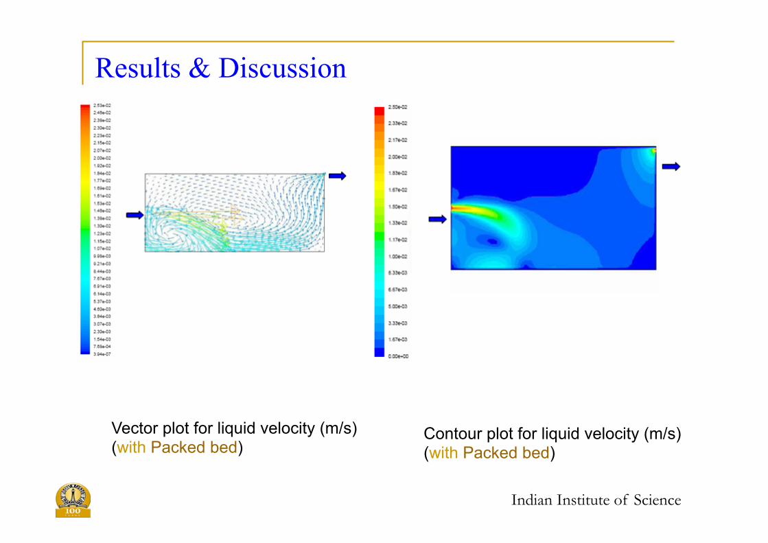
Results & Discussion
Indian Institute of Science
Contour plot for liquid velocity (m/s) (with Packed bed)
Vector plot for liquid velocity (m/s) (with Packed bed)

PIV – experiments
Indian Institute of Science

Experimental verification
Indian Institute of Science
Contours of X-direction mean velocity (inlet NRe=7660) (a)experimental and (b ) Simulation results without packed bed

Experimental verification
Indian Institute of Science
Contours of X-direction mean velocity (inlet NRe=500) (a)experimental and (b ) Simulation results with packed bed

Improving the performance
Indian Institute of Science

Non-ideal flow, mixing and reactions
Indian Institute of Science

Non-ideal flow, mixing and reactions
Indian Institute of Science

Non-ideal flow, mixing and reactions
Indian Institute of Science

Residence time distributions
Ø Exit age distribution E(t)dt q Fraction of material in exit stream which has age
between t and t+dt Ø Cumulative residence time distribution, F(t)
q Fraction of material in exit stream with age less than t
Ø Internal age distribution, I(t)dt q Fraction of material within vessel which has age
between t and t+dt
Indian Institute of Science
0
( )( ) ( ') ' ( ), 1 ( ) ( )'
t dF t VF t E t dt or E t F t I tdt F
= = − =∫
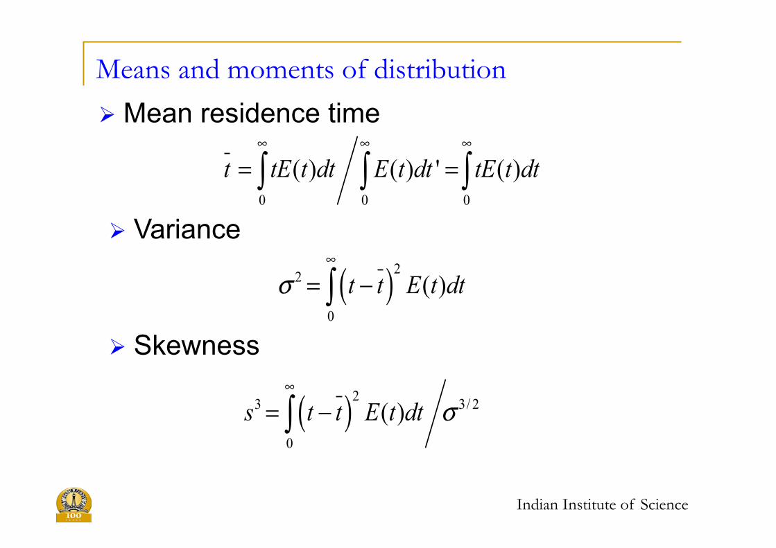
Means and moments of distribution
Ø Mean residence time
Indian Institute of Science
0 0 0
( ) ( ) ' ( )t tE t dt E t dt tE t dt∞ ∞ ∞
= =∫ ∫ ∫Ø Variance
( )22
0
( )t t E t dtσ∞
= −∫Ø Skewness
( )23 3/ 2
0
( )s t t E t dt σ∞
= −∫

Example
Indian Institute of Science
0 2 4 6 8 10 12 140.00
0.05
0.10
0.15
0.20
E
(t)
t0 2 4 6 8 10 12 14
0.0
0.2
0.4
0.6
0.8
1.0
F(t
)
t
0 2 4 6 8 10 12 140.00
0.05
0.10
0.15
0.20
I(t)
t 0 2 4 6 8 10 12 140.0
0.2
0.4
0.6
0.8
t E(t
)
t

Experimental determination of RTD
Ø Convolution integral
Indian Institute of Science
0 0
( ) ( ') ( ') ( ') ( ')t t
e o oC t C t t E t dt C t E t t dt= − = −∫ ∫Ø Pulse input
0
( ) ( ) ( )e eE t C t C t dt∞
= ∫Ø Step input
0( ) ( )eF t C t C=

Determination of RTD from model
Ø CSTR
Indian Institute of Science
( )1( ) expE t t ττ
= −
Ø PFR
( ) ( ), ( ) ( )E t t F t H tδ τ τ= − = −
Ø PFR-CSTR or CSTR-PFR 0
( ) 1 exp
p
pp
s s
tE t t
t
ττ
ττ τ
<= −⎛ ⎞
≥⎜ ⎟⎝ ⎠

RTD and reactions
Ø kinetics of the reaction Ø the RTD of fluid in the reactor Ø the earliness or lateness of fluid mixing in the
reactor Ø whether the fluid is a micro or macro fluid
Indian Institute of Science

Example – second order reaction
Indian Institute of Science
0 2 4 6 8 100.0
0.2
0.4
0.6
0.8
1.0C
/C0
kτC0
CSTR-PF PF-CSTR PF CSTR PF(τ=4) CSTR(τ=4)

Macro- and Micromixing
Ø Macromixing – distribution of residence times in the reactor
Ø Micromixing – description of how molecules of different ages interaction with each other q Complete segregation – all molecules of same
age group remain together until they exit the reactor
q Complete micromixing – molecules of different age group are completely mixed
Ø the earliness or lateness of fluid mixing in the reactor
Ø whether the fluid is a micro or macro fluid Indian Institute of Science

Zero parameter models
Ø Complete segregation
Indian Institute of Science
0
( ) ( )sC C t E t dt∞
= ∫

Model
Indian Institute of Science
00
( ) (0) ( ) ( )
( ) ( ) (0) 0
s
ss
dC R C C C C C t E t dtdtdC C t E t Cdt
∞
= = =
= =
∫
( ) ( ) ( )
( )
( )
2
2
2
0, 0,1 11( )
1( 1 )1
s
z dC dC dz dct t z zz dt dz dt dz
dC R Cdz zdC E z z Cdz z
= ∞ ≡ = = −−
=−
−=−

Zero parameter models
Ø Maxiumum mixedness
Indian Institute of Science
( )10 10( )( ) ( 0)
1 ( )dC ER C C C C Cd F
λ λλ λ= − − − = =
−

Example – second order reaction
Indian Institute of Science
0.01 0.1 1 10 100 1000
0.0
0.2
0.4
0.6
0.8
1.0 maximum mixedness complete segregation 2 CSTRs
C/C
0
kτC0
1 10 100 10000.0
0.2
0.4 maximum mixedness complete segregation 2 CSTRs

Example – mass transfer and reaction
Indian Institute of Science
1 10 100 1000 100000.0
0.1
0.2
0.3
0.4
0.5
0.6
CA
e
r(µm)
maximum mixedness segregated flow
0 2 4 6 8 10
0.0
0.2
0.4
0.6
0.8
1.0
Con
cent
ratio
nθ
CA (r=1µm) CB
CA (r=100µm) CB

One parameter models
Ø Tanks – in - series
Indian Institute of Science
12 1( ) exp
( 1)!
N n
NN t ntE tN N
στ τ
− ⎛ ⎞= =⎜ ⎟− ⎝ ⎠

One parameter models
Ø Axial dispersion model
Indian Institute of Science
( )2 1 11 1 PeePe Pe
σ −⎡ ⎤= − −⎢ ⎥⎣ ⎦

RTD
Indian Institute of Science
0 20.0
0.2
0.4
0.6
0.8
1.0
1.2
1.4
1 2 3 4
10
4
2
1
E(t)
t
0.0 0.5 1.0 1.5 2.00
1
2
3
4
5
6
7
dispersion model500
4050
E(t)
t

Transient in PFR
Indian Institute of Science
0.0 0.2 0.4 0.6 0.8 1.00.0
0.2
0.4
0.6
0.8
1.0 t
0 0.25 0.5 0.75
: :
2.5
C
z

Compartment models
Indian Institute of Science

Example
Indian Institute of Science
0.0 0.2 0.4 0.6 0.8 1.00.0
0.2
0.4
0.6
0.8
1.0
Yie
ldB
ρ
1 CSTR 2 CSTR
0.0 0.2 0.4 0.6 0.8 1.00.0
0.2
0.4
0.6
0.8
1.0
Con
vers
ion A
ρ
1 CSTR 2 CSTR

Indian Institute of Science
Rate contours –reversible reaction
0
0
0
00
0.1
0.1
0.1
0.1
0.1
1
1
11
10
1010
100100
Temperature
α'
300 310 320 330 340 350 360 370 380 390 4000
0.1
0.2
0.3
0.4
0.5
0.6
0.7
0.8
0.9
1
Indian Institute of Science
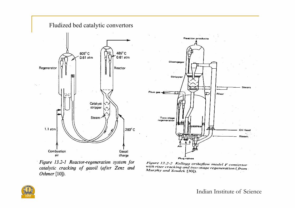
Fludized bed catalytic convertors
Indian Institute of Science
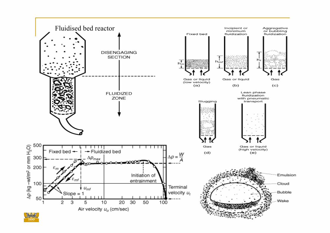
Fluidised bed reactor

Indian Institute of Science
Solid volume fraction