CHEMICAL MASS BALANCE RECEPTOR MODELVERSION 8 (CMB8) USER’S MANUAL

Desert Research Institute Document No. 1808.1D1December, 1997

Prepared by

John G. Watson1

Norman F. Robinson1

Charles Lewis2

Thomas Coulter2

With assistance from

Judith C. Chow1

Eric M. Fujita1

Douglas H. Lownethal1

Teri L. Conner2

Ronald C. Henry3

Robert D. Willis4

1Desert Research Institute, PO Box 60220, Reno, NV 895062US Environemental Protection Agency3University of Southern California4ManTech, Inc.

i

DisclaimerThis manual was prepared as part of Contract 5D1808NAEX between the U.S.

Environmental Protection Agency and the Desert Research Institute of the University andCommunity College System of Nevada. The information presented here does necessarilyexpress the views or policies of the U.S. Environmental Protection Agency or the State ofNevada. The mention of commercial hardware and software in this document does notconstitute endorsement of these products. No explicit or implied warranties are given for thesoftware and data sets described in this document.

ii

Abstract

The Chemical Mass Balance (CMB) air quality model is one of several receptormodels that have been applied to air resources management. CMB8 is a Windows 95 basedversion of CMB modeling software that substantially facilitates the estimation of sourcecontributions to specieated PM10 (particles with aerodynamic diameters less than 10 µm),PM2.5 (particles with aerodynamic diameters less than 2.5 µm), and Volatile OrganicCompound (VOC) data sets. This manual introduces CMB8 and its development history. Itdescribes minimal and desired hardware and software requirements and shows how to installCMB8 on a personal computer. It explains CMB8 menu options and input and output fileformats. The manual provides a step-by step tutorial of CMB8 operations using the exampledata sets provided with the model. Performance measures are briefly described, though theiruse in practical applications is deferred to a separate applications and validation protocol. Asignificant bibliography of CMB-related literature is included for those desiring moreinformation about the CMB, its utility and applications.

iii

Acknowledgements

CMB8 software has been under development since 1995 and has benefited from betatesting since 1996 by many users from all over the world who are too numerous to identifyhere. Further suggestions are welcome from other users, and can be directed to NormanRobinson at normr@sage.dri.edu. Norman Mankim and Mary MacLaran of DRI’s staffprovided publications support for the production and distribution of this manual and thecompilation of references.

iv

Table of Contents

1. Introduction....................................................................................................................1-11.1 CMB8 Features ....................................................................................................1-11.2 Chemical Mass Balance Overview .......................................................................1-21.3 CMB Software History.........................................................................................1-51.4 Organization of User’s Manual.............................................................................1-6

2. Software Installation.......................................................................................................2-12.1 Hardware and Operating System ..........................................................................2-12.2 CMB Software .....................................................................................................2-12.3 Installing CMB8 Software....................................................................................2-2

3. CMB8 Commands.......................................................................................................3-13.1 File Menu Commands ..........................................................................................3-13.2 Main Menu Commands ........................................................................................3-23.3 Graph ...................................................................................................................3-8

4. Input and Output Files ....................................................................................................4-14.1 File Naming Conventions.....................................................................................4-14.2 Input Files ............................................................................................................4-2

4.2.1 Input Filename File: INXXXXYY.IN8 .......................................................4-24.2.2 Source (SO*.SEL), Species (PO*.SEL), and Sample Selection

(DS*.SEL) Input Files.................................................................................4-34.2.3 Ambient Data Input File (AD*.CSV, AD*.DBF, AD*.TXT

AD*.WKS) .................................................................................................4-54.2.4 Source Profile Input File (PR*.CSV, PR*.DBF, PR*.TXT, PR*.WKS).......4-7

4.3 Output Files..........................................................................................................4-74.3.1 Report Output File: RPXXXXRP.TXT ......................................................4-84.3.2 Data Base Output File .................................................................................4-8

4.4 Creating Data Input Files......................................................................................4-84.5 Reading Output Files............................................................................................4-9

5. Using CMB8...............................................................................................................5-15.1 Start CMB8..........................................................................................................5-15.2 Select Data Set .....................................................................................................5-15.3 Examine the CMB8 Banner..................................................................................5-15.4 Set Options...........................................................................................................5-25.5 Select Samples .....................................................................................................5-35.6 Select Fitting Species and Profiles........................................................................5-45.7 Perform CMB Calculation and Review Results ....................................................5-55.8 Examine Performance Measures...........................................................................5-65.9 Autofit..................................................................................................................5-85.10Examine Source Profiles and Receptor Concentrations.........................................5-8

v

5.11Graph Source Profiles, Ambient Concentrations, and Source Contributions..........5-85.12Plot Spatial Pies ...................................................................................................5-95.13Exit CMB8...........................................................................................................5-95.14Working with Large Amounts of Data................................................................5-10

6. CMB Performance Measures..........................................................................................6-16.1 Source Contribution Estimates Display.................................................................6-16.2 Eligible Space Display..........................................................................................6-36.3 Species Concentration Display .............................................................................6-46.4 Additional Performance Measures........................................................................6-5

7. References......................................................................................................................7-1

1-1

1. INTRODUCTION

The Chemical Mass Balance (CMB) air quality model is one of several receptor modelsthat have been applied to air resources management. Receptor models use the chemical andphysical characteristics of gases and particles measured at source and receptor to both identify thepresence of and to quantify source contributions to receptor concentrations. Receptor models aregenerally contrasted with dispersion models that use pollutant emissions rate estimates,meteorological transport, and chemical transformation mechanisms to estimate the contribution ofeach source to receptor concentrations. The two types of models are complementary, with eachtype having strengths that compensate for the weaknesses of the other.

This manual describes how to operate CMB Version 8 (CMB8) modeling software tocalculate source contributions to ambient PM10 (particles with aerodynamic diameters less than 10µm), PM2.5 (particles with aerodynamic diameters less than 2.5 µm), and Volatile OrganicCompounds (VOCs).

A separate applications and validation protocol (Watson et al., 1998) describes how toapply CMB8 to specific situations and how to evaluate its outputs. Several review articles,books, and conference proceedings provide additional information about the CMB and otherreceptor models (Chow et al., 1993; Gordon, 1980, 1988; Hopke and Dattner, 1982 ; Hopke,1985, 1991; Pace, 1986, 1991; Stevens and Pace, 1984; Watson, 1979; 1984, 1989, 1990, 1991).

1.1 CMB8 Features

CMB8 replaces CMB7 (U.S. EPA, 1989; Watson et al., 1990) as a more convenientmethod of estimating contributions from different sources to ambient chemical concentrations. CMB8 returns the same results of CMB7, but it operates in a Windows-base environment andaccepts inputs and creates outputs in a wider variety of formats than CMB7. The major CMB8enhancements are:

• Windows-based, menu-driven operations: CMB commands may be executed withhot-keys, drop down menus, or toolbar buttons.

• Multiple defaults for fitting source, fitting species, and sample selection: Up toten combinations of fitting source profiles and fitting species may be specified in inputdata selection files. Different defaults can be selected with radio buttons duringCMB8 operation. Subsets of source profiles, species, and samples may be specified inselection files to be selected from profile and ambient concentration data files.

• Improved memory management: CMB8 memory is limited only by the availableRAM on the computer, not by pre-set memory limitations.

• Flexible input and output formats: Comma-separate value (CSV), xBASE (DBF),and worksheet (WKS) formats are support as input and output files, in addition to theblank-delimited ASCII text files (TXT) supported by CMB7.

1-2

• Improved graphics: Sample pie plots, spatial pie plots, time series stacked barcharts, source profile bar charts, and ambient concentration bar charts can be createdwithin CMB8. These can be cut from their CMB8 windows and pasted into otherWindows documents.

• Improved collinearity diagnostics: The uncertainty/similarity clusters have beenreplaced with an singular value composition eligible space treatment that allows theuser to define an acceptable error and an acceptable collinearity among weightedsource profiles.

• Automatic decision-making: CMB8 calculations can be automated to eliminatenegative contributions and to select a default set of profiles based on a weightedoptimization of performance measures.

• User-set preferences: Output directories, output file names, positions of decimalpoints in output, output formats, automatic calculation alternatives, performancemeasure weights, eligible space tolerances, receptor concentration units, and maximumiterations for convergence can be set by the user.

• Retention from previous sessions: Options and window position preferencesestablished in one session are carried over into subsequent sessions.

CMB8 differs from CMB7 in the following:

• CMB8 no longer supports CMB6 style ambient data and source profile data files.

• Filename, source profile, ambient data, and sample selection file formats differ slightlyfrom CMB7. CMB7 source profile and ambient concentration data files can be readdirectly by CMB8, however, so backward compatibility is assured.

• Graphical output is no longer provided as HPGL text files. Instead output can beprinted through Windows or copied to the clipboard for insertion into documents. Text output can also be directed to the printer, the clipboard, or a report file.

1.2 Chemical Mass Balance Overview

The CMB receptor model (Friedlander, 1973; Cooper and Watson, 1980; Gordon, 1980,1988; Watson, 1984; Watson et al., 1984; 1990; 1991; Hidy and Venkataraman, 1996) consists ofa solution to linear equations that express each receptor chemical concentration as a linear sum ofproducts of source profile abundances and source contributions. The source profile abundances(i.e., the mass fraction of a chemical or other property in the emissions from each source type)and the receptor concentrations, with appropriate uncertainty estimates, serve as input data to theCMB model. The output consists of the amount contributed by each source type represented by aprofile to the total mass and each chemical species. The CMB calculates values for thecontributions from each source and the uncertainties of those values. The CMB is applicable to

1-3

multi-species data sets, the most common of which are chemically-characterized PM10 (suspendedparticles with aerodynamic diameters less than 10 µm), PM2.5 (suspended particles withaerodynamic diameters less than 2.5 µm), and VOC (Volatile Organic Compounds).

The CMB modeling procedure requires: 1) identification of the contributing sourcestypes; 2) selection of chemical species or other properties to be included in the calculation; 3)estimation of the fraction of each of the chemical species which is contained in each source type(source profiles); 4) estimation of the uncertainty in both ambient concentrations and sourceprofiles; and 5) solution of the chemical mass balance equations. The CMB is implicit in all factoranalysis and multiple linear regression models that intend to quantitatively estimate sourcecontributions (Watson, 1984). These models attempt to derive source profiles from thecovariation in space and/or time of many different samples of atmospheric constituents thatoriginate in different sources. These profiles are then used in a CMB to quantify sourcecontributions to each ambient sample.

Several solutions methods have been proposed for the CMB equations: 1) single uniquespecies to represent each source (tracer solution) (Miller et al., 1972); 2) linear programmingsolution (Hougland, 1973); 3) ordinary weighted least squares, weighting only by precisions ofambient measurements (Friedlander, 1973; Gartrell and Friedlander,1975); 4) ridge regressionweighted least squares (Williamson and DuBose, 1983); 5) partial least squares (Larson andVong, 1989; Vong et al., 1988); 6) neural networks (Song and Hopke,1996); and 7) effectivevariance weighted least squares (Watson et al., 1984).

The effective variance weighted solution is almost universally applied because it: 1)theoretically yields the most likely solutions to the CMB equations, providing model assumptionsare met; 2) uses all available chemical measurements, not just so-called “tracer” species; 3)analytically estimates the uncertainty of the source contributions based on precisions of both theambient concentrations and source profiles; and 4) gives greater influence to chemical specieswith higher precisions in both the source and receptor measurements than to species with lowerprecisions. The effective variance is a simplification of a more exact, but less practical, generalizedleast squares solution proposed by Britt and Luecke (1973)

CMB model assumptions are: 1) compositions of source emissions are constant over theperiod of ambient and source sampling; 2) chemical species do not react with each other (i.e., theyadd linearly); 3) all sources with a potential for contributing to the receptor have been identifiedand have had their emissions characterized; 4) the number of sources or source categories is lessthan or equal to the number of species; 5) the source profiles are linearly independent of eachother; and 6) measurement uncertainties are random, uncorrelated, and normally distributed.

The degree to which these assumptions are met in applications depends to a large extenton the particle and gas properties measured at source and receptor. CMB model performance isexamined generically, by applying analytical and randomized testing methods, and specifically foreach application by following an applications and validation protocol. The six assumptions arefairly restrictive and they will never be totally complied with in actual practice. Fortunately, theCMB model can tolerate reasonable deviations from these assumptions, though these deviations

1-4

increase the stated uncertainties of the source contribution estimates (Cheng and Hopke, 1989;Currie et al., 1984; deCesar et al., 1985, 1986; Dzubay et al., 1984; Gordon et al., 1981; Henry,1982, 1992; Javitz and Watson, 1986; Javitz et al., 1988a, 1988b; Kim and Henry,1989;Lowenthal et al., 1987, 1988a, 1988b, 1988c, 1992, 1994; Watson, 1979).

The formalized protocol for CMB model application and validation (Pace and Watson,1987; Watson et al., 1991; 1998) is applicable to the apportionment of gaseous organiccompounds and particles (Watson et al., 1994a; Fujita et al., 1994). This seven-step protocol: 1)determines model applicability; 2) selects a variety of profiles to represent identified contributors;3) evaluates model outputs and performance measures; 4) identifies and evaluates deviations frommodel assumptions; 5) identifies and corrects of model input deficiencies; 6) verifies consistencyand stability of source contribution estimates; and 7) evaluates CMB results with respect to otherdata analysis and source assessment methods.

The CMB is intended to complement rather than replace other data analysis and modelingmethods. The CMB explains observations that have already been taken, but it does not predictthe future. When source contributions are proportional to emissions, as they often are for PM andVOCs, then a source-specific proportional rollback (Barth, 1970; Cass and McCrae, 1981; Changand Weinstock, 1975; deNevers, 1975) is used to estimate the effects of emissions reductions. Similarly, when a secondary compound apportioned by CMB is known to be limited by a certainprecursor, a proportional rollback is used on the controlling precursor. The most widespread useof CMB over the past decade has been to justify emissions reduction measures in PM10 non-attainment areas. More recently, the CMB has been coupled with extinction efficiency receptormodels (Lowenthal et al., 1994; Watson and Chow, 1994) to estimated source contributions tolight extinction and with aerosol equilibrium models (Watson et al., 1994b) to estimate the effectsof ammonia and oxides of nitrogen emissions reductions on secondary nitrates.

The CMB model does not explicitly treat profiles that change between source andreceptor. Most applications use source profiles measured at the source, with at most dilution toambient temperatures and <1 minute of aging prior to collection to allow for condensation andrapid transformation. Profiles have been “aged” prior to submission to the CMB using aerosoland gas chemistry models to simulate changes between source and receptor (Friedlander, 1981;Lin and Milford, 1994; Venkatraman and Friedlander, 1994). These models are often overlysimplified, and require additional assumptions regarding chemical mechanisms, relativetransformation and deposition rates, mixing volumes, and transport times.

The CMB model requires species with different abundances in different source types, andabundances that do not vary by more than approximately ±100% among source types. Theconsistency of a species abundance is more important than the uniqueness for sourcequantification. The uniqueness is useful to identify which sources to include in a CMB.Combining particle and gas properties for source emissions, normalized to NMHC (non-methanhydrocarbon) or PM2.5 mass emissions, could assist the apportionment of both VOCs and PM2.5.

New analytical methods, however, such as isotopic abundances, specific organiccompounds, and single particle morphology may be used in the CMB when they have been

1-5

applied to source and receptor samples to more precisely differentiate among contributions fromdifferent sub-types. The CMB performs tests on ambient data and source profiles that tell howwell source-type contributions can be resolved from each other for different combinations ofsource profiles and chemical measurements.

The CMB model quantifies contributions from chemically distinct source-types rather thancontributions from individual emitters. Sources with similar chemical and physical propertiescannot be distinguished from each other by the CMB. The CMB model calculates sourcecontribution estimates for each individual ambient sample. The combination of source profilesthat best explains the ambient measurements may differ from one sample to the next owing todifferences in emission rates (e.g., some days may have wood-stove burning bans in effect andothers will not), wind directions (e.g., a downwind point source would not be expected to becontributing at an upwind sampling site), and changes in emissions compositions (e.g., differentgasoline characteristics and engine performance in winter and summer may result in differentprofiles).

1.3 CMB Software History

The Chemical Mass Balance (CMB) receptor model was first applied by Winchester andNifong (1971), Hidy and Friedlander (1972), and Kneip et al. (1972). The original applicationsused unique chemical species associated with each source-type, the so-called "tracer" solution. Friedlander (1973) introduced the ordinary weighted least-squares solution to the CMBequations, and this had the advantages of relaxing the constraint of a unique species in eachsource-type and of providing estimates of uncertainties associated with the source contributions. The ordinary weighted least squares solution was limited in that only the uncertainties of thereceptor concentrations were considered; the uncertainties of the source profiles, which aretypically much higher than the uncertainties of the receptor concentrations, were neglected.

The first user-oriented software for the CMB model was programmed in 1978 at theOregon Graduate Center in FORTRAN IV on a PRIME 300 minicomputer (Watson, 1979). ThePRIME 300 was limited to 3 megabytes of storage and 64 kilobytes of random access memory. CMB Versions 1 through 6 updated this original version and were subject to many of thelimitations dictated by the original computing system. CMB7 was completely rewritten in acombination of the C and FORTRAN languages to operate on microcomputers with floating-point coprocessors, hard disk systems with tens of megabytes storage, and available memory of640 kilobytes. CMB8 upgrades the DOS character-based CMB7 to a Windows graphical userinterface through the use of the programming language Delphi. Source code is in the publicdomain and is available for modification.

1.4 Organization of User’s Manual

Section 1 introduces CMB8 and the scope of this manual. Section 2 describes minimaland desired hardware and software requirements and shows how to install CMB8 on a personalcomputer. Section 3 describes CMB8 menu options while Section 4 documents input and outputfile formats. Section 5 provides a step-by step tutorial of CMB8 operations using the example

1-6

data sets provided with the model. Performance measures are briefly described in Section 6,though their use in practical applications is deferred to a separate document (Watson et al., 1998). Section 7 includes a bibliography of CMB-related literature, including references citedthroughout this software manual.

2-1

2. SOFTWARE INSTALLATION

This section describes the hardware requirements, computer programs, and installationprocedures for CMB8.

2.1 Hardware and Operating System

The minimum requirements for running CMB8 software are:

• IBM PC compatible desktop, portable, or laptop computer with 386 processor and 8MB RAM

• Hard disk drive with 100 MegaBytes

• MS Windows 3.1 or higher operating system

The recommended hardware configuration is:

• IBM compatible Intel Pentium microcomputer with 32 MB of RAM.

• Super VGA video graphics adapter and monitor.

• Graphics capable printer.

• Windows 95 or Windows NT operating system.

2.2 CMB Software

CMB8 software can be acquired from the National Technical Information Service or it canbe retrieved from the EPA's Support Center For Regulatory Air Models Bulletin Board System(SCRAM BBS), or the EPA’s FTP site

ttnftp.rtpnc.epa.gov:/e-drive/scram/cmb8/

The following files are available and can be downloaded as needed:

• CMB832.EXE: A self-extracting compressed file containing the executable CMBcode and supporting windows files for 32-bit operating systems. This includes allapplications using Windows 95 and Windows 3.1 that have been upgraded to 32-bitprocessing. This is the file that should be downloaded unless one is using an older,and currently unsupported, 16-bit Windows 3.1 operating system.

• CMB816.EXE: A self-extracting compressed file with the same contents asCMB832.ZIP except that it operates on Windows 3.1 16-bit operating systems. Thisversion is included only for backward compatibility. Most users do not need this file.

2-2

• CMB8MAN.EXE: A self-extracting compressed file containing an Adobe Acrobat(CMB8MAN..PDF) file and Microsoft Word 97 (CMBDOC?.DOC) files of thisUser’s Manual. Use this manual to learn CMB8 features and operating methods.

• CMB8DPOR.EXE: A self-extracting compressed file of the example PM10 data inPortland, OR, from the Portland Aerosol Characterization Study (Watson et al., 1979)used to demonstrate basic CMB8 model features in this manual. This example isidentical to that used for CMB7.

• CMB8DSJV.EXE: A self-extracting compressed file of example PM2.5 data fromseveral sites in California’s San Joaquin Valley Air Quality Study (VAQS, Chow et al.,1990; 1992) that is used in the example application in Section 5 of this manual.

• CMBDNAR.EXE: A self-extracting compressed file of example hydrocarboncanister data in Boston, MA, from the North American Regional Study ofTropospheric Ozone (NARSTO) VOC source apportionment in Boston, MA (Fujita etal., 1997) that shows how files can be set up for VOC canister measurements.

• CMBDHOU.EXE: A self-extracting compressed file of example continuous (hourly)hydrocarbon measurements in Houston, TX, from the Coastal Oxidants AtmosphericStudy (Fujita et al., 1995).

• CMB8SOR.EXE: A self-extracting compressed file of CMB source code. This filepreserves the source code for further updates and allows it to be inspected forscientific verification. Most users do not need this file. CMB8 software is written inthe C, FORTRAN, and Delphi computer languages. The executable files are producedusing compilers from Borland (Delphi), Watcom (16 bit C and FORTRAN), andMicrosoft (32 bit C and FORTRAN).

The examples given in this manual are specific to the Windows 95 installation and use ofthe 32-bit software. These examples can be followed for Windows 95 or the installation of the16-bit software, though the illustrated displays will appear different.

2.3 Installing CMB8 Software

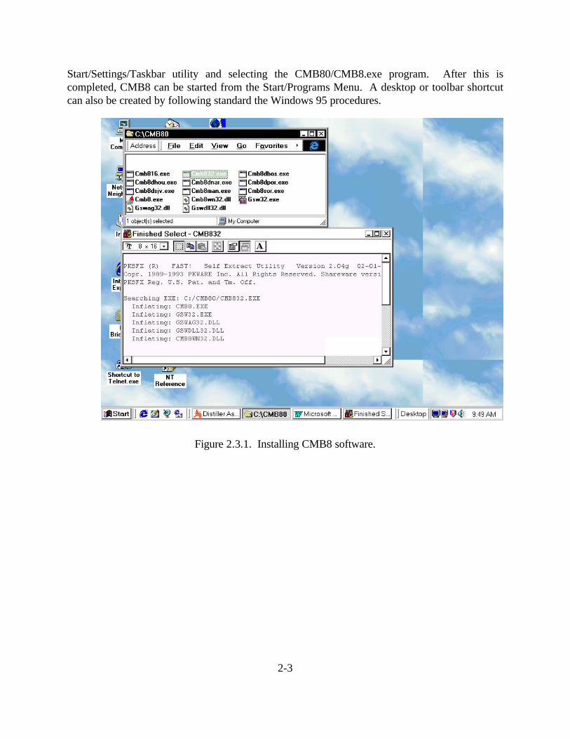
Create a folder entitled CMB80 and transfer the CMB832.EXE file into the folder. Double-click the mouse on the CMB832.EXE icon and the needed software will self-extract tocreate the operations files, as shown in Figure 2.3.1. The other compressed files for test data setsand instructions can be also be obtained by double-clicking on the appropriate icon. icons. The*.DLL and other executable files that accompany CMB8.EXE must be present in the samedirectory for the program to properly execute.

The most convenient way to start CMB8 is to open the CMB8 folder and double-click onthe CMB8 icon. CMB8 may also be installed by using the Add/Remove Program utility on theWindows 95 Control Panel. It can also be added to the Windows 95 Start Menu by clicking the

2-3

Start/Settings/Taskbar utility and selecting the CMB80/CMB8.exe program. After this iscompleted, CMB8 can be started from the Start/Programs Menu. A desktop or toolbar shortcutcan also be created by following standard the Windows 95 procedures.

Figure 2.3.1. Installing CMB8 software.

3-1

3. CMB8 COMMANDS

This section describes the CMB model commands. The appearance of example screensmay differ slightly from those seen during an actual application owing to differences in hardwareand software configurations.

CMB8 commands can be selected from drop down menus, the tool bar, or by usingkeyboard shortcuts. The 3-letter mnemonic is supplemented by a reminder when the cursor inplaced over the button. Below the tool bar is a status bar where the currently selected ambientdata record is displayed and an indication of whether a fit has been done on the currently selectedambient data record is displayed.

3.1 File Menu Commands

Figure 3.1.1 shows the File menu options that are accessed by clicking on the Filemnemonic with the mouse arrow. ALT-F can also be used to access this menu using thekeyboard. Keyboard shortcuts for all menu items are underlined.

Figure 3.1.1. File menu options.

3-2

The file menu options are:

• CMB8 Input File Names (CTRL-I): Selection of this item brings up a window forselection of a input file names file. The function of this file is identical to that of theinput file names file prompted for upon program invocation, and this menu item maybe used to start a new session without the need to exit and restart the program.

• Exit (CTRL-X): Selection of this item terminates the program.

3.2 Main Menu Commands

The main menu, shown in Figure 3.2.2 contains the commands that are most commonlyused to perform CMB calculations and evaluate performance.

Figure 3.2.1. Main menu options.

These commands are described below with their shortcut keys and Toolbar buttons.

• Select Samples (SAM, CTRL-M): The sub-set of samples on which CMB sourceapportionments will be performed is selected by this command. Select or deselect anambient data record by clicking on the desired ambient data record item. Selection is

3-3

indicated by the presence of the asterisk. Click the Select All or Deselect All button toselect or deselect all samples, respectively. Click the OK button to record theselection and deactivate the menu; the sample selection menu must be deactivated toprogress further with the program. Upon leaving this menu the first selected ambientdata record is defined to be the current ambient data record and CMB fits areperformed on it. The sample selection window, as well as other windows, may bemoved to other locations on the desktop.

• Select Species (SPE, CTRL-E): Fitting species are used in the calculation of sourcecontribution estimates. Species not included in this calculation are termed floatingspecies. The comparison of calculated and measured values for floating species is partof the model validation process. Fitting species should be selected that are major orunique components of the source-types influencing the receptor concentrations.Default fitting species are selected in the species selection input file (e.g.PO????.SEL) and are indicated by an asterisk next to the species name. The Select Allor Deselect All buttons designate all or none of available choices as fitting species.Click on an individual species mnemonic to select or deselect it, as indicated by thepresence or absence of an asterisk. This window may be left open during a CMBsession and can be resized and moved to a convenient location on the Windowsdesktop. Click the Close button to remove it. Click the Defaults button to select fromup to ten different combinations of fitting species specified in species selection inputfile. Click the Modify button to modify any of the default selections. Click the OKbutton to deactivate the defaults window, which is required for further progress.

• Select Sources (SRC, CTRL-S): Fitting source profiles are included in the CMBcalculation and are selected to represent the emissions most likely to influence receptorconcentrations.. Several profiles may be available that represent the same source-type,but only one of these is usually used as a fitting source. Profiles of similar chemicalcomposition are often found to be collinear when two or more are selected as fittingsources. Default fitting species are selected in the profile selection input file (e.g.SO????.SEL) and are indicated by an asterisk next to the source mnemonic. TheSelect All or Deselect All buttons designate all or none of available choices as fittingsources. Click on an individual source mnemonic to select or deselect it, as indicatedby the presence or absence of an asterisk. This window may be left open during aCMB session and can be resized and moved to a convenient location on the Windowsdesktop. Click the Close button to remove it. Click the Defaults button to select fromup to ten different combinations of fitting sources specified in profile selection inputfile. Click the Modify button to modify any of the default selections. Click the OKbutton to deactivate the defaults window, which is required for further progress.

• Advance Samples (ADV, CTRL-V): This action retrieves data from the next samplein the sample selection list. It is used after a satisfactory CMB calculation has beencompleted and the results recorded. Note that the sample identification informationbelow the toolbar changes to identify the current sample being analyzed.

3-4

• Calculate Source Contributions (FIT, CTRL-U): This action performs the least-squares estimation of source contribution estimates and performance measures on theselected sample data using the designated fitting species and source profiles. Of noteis the way CMB8 handles missing values in source and receptor files (designated by –99 in place of the value). When a fitting species value is missing in CMB8, thatspecies is automatically removed from the calculation and the species selection flat isset to “M” in the report output file. If this procedure results in more fitting sourcesthan fitting species an error message is written, and all fitting sources and calculatedspecies are set to missing values. The FIT command causes source contributionestimates and performance measures to appear in the output window.

• Show Fit (SHO, CTRL-W): This command displays output from the most recentCMB calculation in the output window. This is useful for reviewing results after thewindow has been cleared. The contents of the output window can also be selectedwith the left mouse button and copied from pop-up menu that appears when the rightmouse button is clicked. The output window can be sized and re-located on theWindows desktop where it will appear in the current and subsequent sessions. Severaltoolbar buttons appear at the bottom of the output window that perform variousfunctions as shown in Figure 3.2.2.

Figure 3.2.2 Toolbar buttons in the CMB8 Output window.

– Clear: Erases all material currently printed in the Output window. The Outputwindow cannot retain more than 32 Kbytes of information and must be periodicallycleared during a CMB session.

– Clear Last: Erases only the most recent output appearing in the Output window.This button may be repeatedly selected and the program will progress backthrough the output text blocks, clearing each in turn.

– Write RP: Writes the entire contents of the Output window to the report outputfile (default CMBOUTRP.TXT).

– Write Last : Writes the most recent addition to the Output window into thereport output file. Write Last is used to record the final source contributionestimates for a sample along with the fitting species and source profile selectionsapplied to obtain those contributions. It is also used to record the most recentinformation from other CMB commands that is displayed in the output window.

– Write DB: Writes the results of the most recent fit to the data base output file(default CMBOUTDB.TXT). The data base format includes records of sourcecontributions to each measured species for each sample.

3-5

– Print: Prints the entire contents of the display window using the current Windows95 printer setting as defined by the Print Manager. Windows 95 also allows printeroutput to be directed to a file. For all three of the Write buttons the user isprompted for confirmation before an existing file is overwritten. The Courier 12point font used in the Output display correctly aligns columns and is the defaultWindows 3.1 and HP LaserJet font.

– Print Last: Prints only the most recent addition to the Output window.

– Close: Closes the Output window.

• Autofit (AUT, CTRL-A): Autofit allows a single selection of fitting species andprofiles to be applied to a selected list of samples without operator intervention. Thisfeature is especially useful for model simulation testing and screening purposes. Autofit displays the Select Samples menu from which the desired samples are selected.It calculates source contribution estimates for each sample using the currently-selectedfitting species, source profiles, and calculation options. After calculation, Autofitwrites the results to the report and data base output files.

• Present Source Contributions (SCN, CTRL-O): This command presents a screendisplay of the fractional contribution of each source-type to each chemical species. These results are useful when contributions to species other than total mass aredesired. This display also indicate which sources are the major and minor contributorsto each chemical concentration.

• Present Computed Averages (AVG, CTRL-L): Averages and standard deviationsof a series of source contribution estimates are calculated and displayed in the Outputwindow. Only source contribution estimates written to the data base output file withthe Write DB command are included in the average. The results of these averages canbe written in the report output file with the Write Last command.

• Present Source Profiles (PRO, CTRL-G): Source profile entries (the mass fractionof each chemical component in each profile) are displayed in the Output window. Thisis useful to verify that input data files have been properly read and to identify theabundant components in each profile. The first row for each species displays thefractional abundance and the second row displays the standard deviation.

• Present Receptor Concentrations (RCN, CTRL-R): Ambient measurements forthe current data record are displayed in the Output Window. This is useful to verifythat input data files have been properly read in.

• Present Normalized MPIN Matrix (MPN, CTRL-N): The Modified Psuedo-Inverse Normalized matrix (MPIN) is displayed in the Output window for the fittingspecies. The MPIN identifies the influence of fitting species on the sourcecontribution estimates.

3-6

• Options (OPT, CTRL-T): Several options and defaults have been added to CMB8that are selected from the Options window, where various values and selections maybe changed from their default values. Option settings are saved in a file namedCMB8RSTR.DAT when the program is closed. This file is read when CMB8 isstarted for subsequent sessions and its contents dictate the new defaults.

Figure 3.2.3 CMB8 Options window.

– Output File Format: Sets the output file formats to blank delimited text(*.TXT), comma separated value (*.CSV), xBASE (*.DBF), or Lotusspreadsheet (*.WKS). Select the radio button that corresponds to the desiredoutput format. The default setting is blank delimited text (*.TXT). xBASEprograms such as dBASE and FoxPro specify that field names begin with analphabetic character, and variable names for input files (source and species codesand mnemonics) must also begin with a letter rather than a number when the DBFformat is for .

– Display Dec’s: Sets the number of decimal places displayed in the output windowand output files. This depends on the units used in the input data files. Forexample, data reported in ng/m3 require fewer decimal places than valuesexpressed in µg/m3. This setting affects the "Show Fit" and "Write RP" displaycolumns for inverse singular values, source contributions estimates, measuredspecies concentrations, and calculated species concentrations. Click the edit boxand type the desired number of decimal places. The default value is 5 and themaximum value is 6.

– Max. Src. Unc. and Min. Src. Proj.: These parameters allow the eligible spacecollinearity evaluation method of Henry (1992) to be implemented with each CMBcalculation. The eligible space method uses: 1) maximum source uncertainty; and

3-7

2) minimum source projection on the eligible space. The maximum sourceuncertainty is expressed as a percentage of the total measured mass and is set to adefault value of 20% in CMB8. The minimum source projection is set to a defaultvalue of 0.95. Maximum source uncertainty defines the eligible space as thatspanned by eigenvectors with inverse singular values less than or equal to themaximum source uncertainty. Sources lying within the eligible space may beestimated with an uncertainty less than the maximum source uncertainty. Thisstrict criteria of inclusion is relaxed somewhat and estimable sources are defined tobe those with projections into the eligible space is at least the minimum sourceprojection. Inestimable sources have small projections within the eligible space. Certain linear combinations of inestimable sources may be estimable, and theprogram lists these, if any exist. This may be understood as removing uncertaintyby combining collinear sources. Different values for the maximum searchuncertainty (ranging from 0 to 100%) and minimum source projections (rangingfrom 0 to 1.0) may be typed into the appropriate edit boxes and will be retained forsubsequent source contribution calculations.

– B and L: Checking this box applies the Britt and Luecke (1973) linear leastsquares solution that is explained by Watson et al., 1984) when applied to CMBcalculations. This option is available for research purposes and is not of utility inpractical CMB applications. Checking the B and L box causes CMB8 to use theBritt and Luecke algorithm when performing the CMB fit.

– S. Elim.: Checking this box eliminates negative source contributions from thecalculation. Fitting sources are eliminated one at a time, in sequential order, withfits performed after each elimination until all source contributions are positive.

– Best Fit: Checking this box cycles between the default fitting species and sourceprofile combinations specified in the source and species selection input files untilthe best composite Fit Measure has been achieved. The first default fitting speciesselection is paired with the first default fitting sources selection, and so on. The fitwith the largest Fit Measure is then displayed and becomes the current fit. After aBest Fit has been made the radio button in the default fitting species window andthe radio button in the default fitting sources window are set to that used in thebest fit.

– Measure Weight: These are the weights applied to each of the performancemeasures chi square, r-square, percent mass, and fraction of eligible sources(number in eligible space divided by number of fitting sources). Weights may bebetween 0 and 10,000 and are entered by typing into the appropriate edit boxes. Defaults are 1.0 for each performance measure.

– RP Name: Renames the default report file (CMBOUTRP.TXT) to any othername by typing into the edit box. If the file already exists, the user is asked forpermission to overwrite the existing file with a new one.

3-8

– DB Name: Renames the default data base file (CMBOUTDB.TXT) to any othername by typing into the edit box. The file extension reflects the output format theedit box.

– Units: The units used in the Fit display may be changed by use of this edit box. The number of characters is limited to 5 or less.

– Working Directory: Output data files are written to the directory specified here. It defaults to the directory in which the CMB8 input files are located. To changethis directory, edit the text in the edit box. This may be done at any time andresults in a new working directory.

3.3 Graph

The graph menu, shown in Figure 3.3.1, allows visual outputs to be obtained for sourceprofiles, ambient concentrations, and source contribution estimates.

Figure 3.3.1. CMB8 Graph menu.

The Graph menu selections are:

3-9

• Species (CTRL-F2): Produces a bar graph of the species concentrations for thecurrently selected sample. The Y axis is a logarithmic scale, the height of the barindicates the CMB8 calculated concentration, a horizontal line represents themeasured concentration, and the error bars indicate the measurement precision. Thegraph adjusts to the size of the window, which can be re-sized by standard windowsmethods.

• Source Profiles (CTRL-F3): A list box appears from which the desired profile can beselected. The Y axis is a logarithmic scale, the height of the bar indicates theabundance of each chemical species, and the error bars indicate the measurementprecision. The graph adjusts to the size of the window, which can be re-sized bystandard Windows methods.

• Source Contributions (CTRL-F4): Produces a pie chart of the source contributionsfor the current sample and the most recently calculated source contribution estimates.

• PM10 (CTRL-F5): Produces a pie chart of the source contributions for size TOTALif the most recent two fits were to sizes FINE and COARS in any order.

• Time Series (CTRL-F6): - Creates a time series of stacked bars representing differentsource contributions. This selection operates calculations made by the most recent useof Autofit. Upon selection of this item the user is prompted for a site if more than oneoccurs among the Autofit sites. Similarly, the user is prompted for a size fraction ifmore than one occurs. A final prompt allows the user to reduce the number of fitsdisplayed.

• Spatial Pies (CTRL-F7): Plots pie charts of source contributions at specified sitecoordinates. This plot is useful for comparing source contributions among differentsites as part of CMB model evaluation. It operates on source contribution estimatescalculated by the most recent Autofit. Upon selection of this item the user isprompted for a date and start hour pair if more than one occurs among the Autofitcalculations. Similarly, the user is prompted for a size fraction if more than oneoccurs. A final prompt allows the user to reduce the number of samples displayed. The remaining source contributions are then presented in a spatial series as pie chartsusing coordinates read from the ambient data selection file. The area of the pie chartsis proportional to the total calculated mass, with the largest area being approximately 1square inch on an 11” by 8.5” scale.

• Close (CTRL-F8): Closes the graphical output window.

The Graph window contains several command buttons, shown in Figure 3.3.2 that areused to record graphical outputs.

3-10

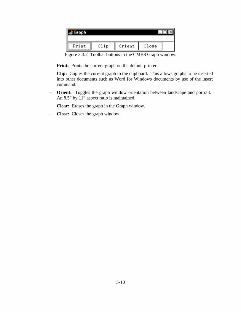
Figure 3.3.2 Toolbar buttons in the CMB8 Graph window.

– Print: Prints the current graph on the default printer.

– Clip: Copies the current graph to the clipboard. This allows graphs to be insertedinto other documents such as Word for Windows documents by use of the insertcommand.

– Orient: Toggles the graph window orientation between landscape and portrait. An 8.5” by 11” aspect ratio is maintained.

Clear: Erases the graph in the Graph window.

– Close: Closes the graph window.

4-1

4. INPUT AND OUTPUT FILES

This section describes the structure of CMB8 input and output files and methods ofgenerating these files. Each type of input file structure is illustrated with one of the test data setspackaged with CMB8.

4.1 File Naming Conventions

CMB input and output files can have any eight-character file name with a three-characterextension that indicates the file type. The most convenient and universal naming convention isPPXXXXYY.SSS, where:

• PP: Type of file. Common definitions are:

– IN-File identifying other input data file names.

– SO-Source profile selection file, identifying default fitting profiles and sourceprofile descriptions.

– PO-Species selection file, identifying default fitting species.

– DS-Data selection file, identifying samples to be selected from the ambient data file for apportionment during a CMB session.

– AD-Ambient data file, containing the measured ambient concentrations and theirprecisions.

– PR-Source profile file, containing mass-fraction chemical abundances and theiruncertainties.

– OU-Output file, containing report or data base output.

• XXXX: Study identifier. This four-letter code allows separate studies to bedistinguished from one another.

• YY: Session or report identifier. This two-letter code can be assigned to variationson input data files or to distinguish report and data base output files. For example,input data files might be divided up by season or by sampling site to be evaluated inseparate CMB modeling sessions. YY might take on the values ‘WI’ for winter, ‘SP’for spring, ‘SU’ for summer, and ‘FA’ for fall. Default output filenames can bedesignated in the options menu with ‘RP’ identifying the report file and ‘DB’representing the data base file. Output files should be written into separate directories,as designated in the Options menu, when different input files are used for the sameproject.

• SSS: File format identifier. The following file extensions are recognized by CMB8:

– IN8: Input filename ASCII text file. CMB8 lists files with this extension when theprogram is executed and when CMB8 input files are requested using the Filemenu.

4-2

– SEL: Fitting profile, fitting species, and sample selection ASCII text files. CMB8recognizes files with this extension has containing default selections that can beentered external to the program. This extension applies only to the SO, PO, andDS file types.

– CSV: Ambient data or source profile comma separated value ASCII text file. Each field is separated by a comma. Comma-delimited ASCII data base outputfiles are written with this extension.

– DBF: X-base data base file generated by dBASE or FoxPro compatible datamanagement software. Most commonly used spreadsheets offer this as an outputoption. DBASE or FoxPro output files are written with this extension.

– TXT: Ambient data or source profile data blank-delimited ASCII text file. Blank-delimited ASCII data base output files are written with this extension.

– DAT: Ambient or source profile data ASCII text file, blank delimited. Filestructure is identical to TXT extensions.

– WKS: Lotus 1-2-3 version 1 spreadsheet format. Most commonly usedspreadsheets offer this as an output option. This is the most useful output formatfor the data base output file when source contribution estimates will be analyzedusing a spreadsheet.

CMB8 converts the CSV, DBF, and WKS input data files to blank-delimited (TXT) filesthat are actually used by the program. This file carries the TXT suffix and may be used insubsequent modeling sessions to minimize startup time.

4.2 Input Files

Six data files are used for input to CMB8. Only the ambient and source profile data filesare required, however. Though optional, the remaining four files provide substantial userconvenience by establishing commonly used defaults and sample subsets that would otherwiseneed to be initialized each time CMB8 is run.

4.2.1 Input Filename File: INXXXXYY.IN8

This fixed format file contains a list of the names of other CMB8 input data files. Thisfilename, which is normally entered in response to the first few prompts when CMB8 is started,consists of five lines as shown below. These lines, in succession, contain the names of the fileswhich are described in the following sub-sections. INSJVF.IN8 is an example of this file structureused in CMB8.

1 201234567890SOSJVF.SELPOSJVF.SELDSSJVF.SELADSJVF.CSVPRSJVF.CSV

4-3

File name entries should be left justified. For the CMB8 32 bit version, the only restrictionon file names is that they are acceptable to the operating system. This means that extended filenames may be used. For the CMB8 16 bit version, each filename can be up to eight characters inlength with up to a three-character suffix, and the fully qualified path plus file name should be lessthan 256 characters in length. The purpose of this file is to save the effort of keying in the inputfilename individually. If an INXXXXYY.IN8 filename is not entered at the appropriate prompt,CMB8 will request the names of individual data input filenames.

4.2.2 Source (SO*.SEL), Species (PO*.SEL), and Sample Selection (DS*.SEL) Input Files

The source, species and sample selection files provide defaults that do not have to beentered from the program each time a CMB8 session is begun. These files limit the profiles,species, and ambient data records to those listed in the selection files, even though a largernumber may be included in the ambient and source profile data files. This means that the data filesneed not be edited when only subsets of variables are desired for a specific CMB8 modelingsession. The source and species selection files also allow default sets of fitting profiles andspecies to be designated, making it unnecessary to select these at the beginning of each CMB8session. Variable definitions can also be documented in these files. Sampling site coordinates canbe documented in the sample selection file.

Following is an example of the source profile selection file SOSJVF.SEL:0 1 2 3 41234567890123456789012345678901234567890SJV001 SOIL01 * STOCKTON AGRICULTURAL SOIL (PEAT)SJV002 SOIL03 * FRESNO PAVED ROADSJV003 SOIL04 VISALIA AG SOIL (COTTON/WALNUT)SJV004 SOIL05 VISALIA AGRICULTURAL SOIL (RAISIN)SJV005 SOIL06 * VISALIA SAND AND GRAVELSJV006 SOIL07 VISALIA URBAN UNPAVEDSJV007 SOIL08 VISALIA PAVED ROADSJV008 SOIL09 BAKERSFIELD AGRICULTURAL SOIL, ALKALINESJV009 SOIL10 BAKERSFIELD AG SOIL, SANDY LOAMSJV010 SOIL11 BAKERSFIELD UNPAVED ROAD (OILDALE)SJV011 SOIL12 * BAKERSFIELD PAVED ROADSJV012 SOIL13 BAKERSFIELD WINDBLOWN URBAN UNPAVEDSJV013 SOIL14 * BAKERSFIELD AG SOIL, WASCO SANDY LOAMSJV014 SOIL15 BAKERSFIELD AG SOIL, CAJON SANDY LOAMSJV015 SOIL16 BAKERSFIELD UNPAVED ROAD (RESIDENTIAL)SJV016 SOIL17 * TAFT UNPAVED ROADSJV017 BAMAJC * * * * * BAKERSFIED CORDWOOD, MAJESTIC FIREPLACESJV018 MAMAJC MAMMOTH LAKES WOOD, MAJESTIC FIREPLACESJV019 MAFISC BAKERSFIELD WOOD, FISHER MAMA BEAR STOVESJV020 MADIEC MAMMOTH LAKES DIESEL TOUR BUSES (IDLING)SJV021 BAAGBC BAKERSFIELD AG BURN (WHEAT AND BARLEY)SJV022 ELAGBC EL CENTRO AGRI. BURN (WHEAT)SJV023 FRCONC FRESNO HIGHWAY 40 CONSTRUCTIONSJV024 STAGBC STOCKTON AGRI. BURN (WHEAT)SJV025 VIAGBC VISALIA AGRI BURN (WHEAT)SJV026 VIDAIC VISALIA DAIRY/FEEDLOT DUSTSJV027 SFCRUC * * * * * SANTA FE CRUDE BOILERSJV028 CHCRUC CHEVRON RACETRACK CRUDE BOILERSJV029 MOTIBC MODESTO TIRE POWER PLANTSJV030 SCRRFC STANISLAUS RESOURCE RECOVERY FACILITYSJV031 CDCEMT NBS CEMENT DUSTSJV032 CDRKCR ROCK CRUSHING 1987 SCAB

4-4

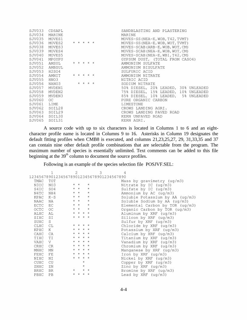
SJV033 CDSAPL SANDBLASTING AND PLASTERINGSJV034 MARINE MARINESJV035 MOVES1 MOVES-SS(NEA-E,WOB,T42,TVMT)SJV036 MOVES2 * * * * * MOVES-SS(NEA-E,WOB,WOT,TVMT)SJV038 MOVES3 MOVES-SCAB(ARB-E,WOB,WOT,CM)SJV039 MOVES4 MOVES-SCAB(NEA-E,WOB,WOT,CM)SJV040 MOVES5 MOVES-SCAB(NEA-E,WB1,T42,CM)SJV041 MPGYPU GYPSUM DUST, (TOTAL FROM CASO4)SJV051 AMSUL * * * * * AMMONIUM SULFATESJV052 AMBSUL AMMONIUM BISULFATESJV053 H2SO4 SULFURIC ACIDSJV054 AMNIT * * * * * AMMONIUM NITRATESJV055 HNO3 NITRIC ACIDSJV056 NANO3 * * * * SODIUM NITRATESJV057 MVDEN1 50% DIESEL, 20% LEADED, 30% UNLEADEDSJV058 MVDEN2 75% DIESEL, 15% LEADED, 10% UNLEADEDSJV059 MVDEN3 85% DIESEL, 10% LEADED, 5% UNLEADEDSJV060 OC PURE ORGANIC CARBONSJV061 LIME LIMESTONESJV062 SOIL28 CROWS LANDING AGRI.SJV063 SOIL29 CROWS LANDING PAVED ROADSJV064 SOIL30 KERN UNPAVED ROADSJV065 SOIL31 KERN AGRI.

A source code with up to six characters is located in Columns 1 to 6 and an eight-character profile name is located in Columns 9 to 16. Asterisks in Column 19 designates thedefault fitting profiles when CMB8 is executed, and columns 21,23,25,27, 29, 31,33,35 and 37can contain nine other default profile combinations that are selectable from the program. Themaximum number of species is essentially unlimited. Text comments can be added to this filebeginning at the 39th column to document the source profiles.

Following is an example of the species selection file POSJVF.SEL:

1 2 3 41234567890123456789012345678901234567890 TMAC TOT Mass by gravimetry (ug/m3) N3IC NO3 * * * Nitrate by IC (ug/m3) S4IC SO4 * * * Sulfate by IC (ug/m3) N4TC NH4 * * * Ammonium by AC (ug/m3) KPAC K-S * * * Soluble Potassium by AA (ug/m3) NAAC NA * * * Soluble Sodium by AA (ug/m3) ECTC EC * * * Elemental Carbon by TOR (ug/m3) OCTC OC * * * Organic Carbon by TOR (ug/m3) ALXC AL * * * * Aluminum by XRF (ug/m3) SIXC SI * * * * Silicon by XRF (ug/m3) SUXC S Sulfur by XRF (ug/m3) CLXC CL * * * * Chloride by XRF (ug/m3) KPXC K * * * * Potassium by XRF (ug/m3) CAXC CA * * * * Calcium by XRF (ug/m3) TIXC TI * * * * Titanium by XRF (ug/m3) VAXC V * * * * Vanadium by XRF (ug/m3) CRXC CR * * * * Chromium by XRF (ug/m3) MNXC MN * * * * Manganese by XRF (ug/m3) FEXC FE * * * * Iron by XRF (ug/m3) NIXC NI * * * * Nickel by XRF (ug/m3) CUXC CU * Copper by XRF (ug/m3) ZNXC ZN * Zinc by XRF (ug/m3) BRXC BR * * * Bromine by XRF (ug/m3) PBXC PB * * * * Lead by XRF (ug/m3)

4-5

A species code with up to six characters is located in Columns 1 to 6 and an eight-character species name is located in Columns 9 to 16. Asterisks in Column 19 designates thedefault fitting species when CMB8 is executed, and columns 21,23,25,27, 29, 31,33,35 and 37can contain nine other default species combinations that are selectable from the program. Themaximum number of species is essentially unlimited. Text comments can be added to this filebeginning at the 39th column to document the meaning and units of the chemical components.

For the ambient data records selection file, columns 1 through 12 are for the site ID,columns 14 through 21 are for the date, columns 23 and 24 for the sample duration, columns 26and 27 for the sample start hour, and columns 29-33 for the particle size fraction, if appropriate. Intermediate columns should be blank. An asterisk in column 35 selects a record. In additioncolumns 37 through 46 and columns 48 through 57 may contain x and y coordinates, respectively,for use in the Spatial Pie plots (see below). These should be in floating point format, e.g.,123.456, and should increase in value from left to right and from bottom to top. UTMcoordinates are suitable as well as fractional longitudes and latitudes, if the longitudes areexpressed as negative numbers.

Following is an example of the species selection file DSSJVF.SEL:

1 2 3 4 5 61234567898012345678901234567890123456789012345678901234567890BAKERS 02/27/89 24 0 FINE * -119.01600 035.35800CROWS 02/27/89 24 0 FINE * -121.13000 037.37500 FELLOW 02/27/89 24 0 FINE * -119.43900 035.13700 FRESNO 02/27/89 24 0 FINE * -119.74000 036.70600 KERN 02/27/89 24 0 FINE * -119.62500 035.59600 STOCKT 02/27/89 24 0 FINE * -121.26700 037.95100

The file structure through the first 5 fields is that of the ambient data input, with columns1-12 for the site name, columns 13-20 for the sample date, columns 22-23 for the sample duration(in hours), columns 25 and 26 for the sample start time (hour beginning), columns 28-32 for theparticle size fraction, column 34 for an asterisk to identify this sample as a section forapportionment, columns 37-45 for the x-coordinate (west-east) of the corresponding samplingsites, and columns 47-55 for the y-coordinate (south-north) of the corresponding site. Sitecoordinates should be selected so that they are of increasing magnitude from west to east andfrom south to north. The negative longitude coordinate in columns 37 through 46 above meetsthat criterion. Coordinates should be in fractional units. UTM coordinates can also be used whenthey are all from the same zone. These coordinates are used for the spatial plotting display. Sitecoordinates are optional, and their columns are ignored if they are left blank. Only the firstreference to a sampling site code requires coordinates to be supplied. These are assumed to beconstant for all subsequent references to this site code.

4.2.3 Ambient Data Input File (AD*.CSV, AD*.DBF, AD*.TXT AD*.WKS)

Ambient data files may be formatted as column-separated values in ASCII text (CSV),xBASE (DBF), blank-delimited ASCII text (TXT), or Lotus Worksheet (WKS). The CSV andDBF formats are preferred, as they are easier to prepare in spreadsheet (e.g. Microsoft Excel,Corel QuatroPro, Lotus 123) and data base (e.g. Microsoft Access, dBASE) software than the

4-6

other formats. The WKS format creates large files and requires substantial translation time forCMB8 input and output, so it is the least desirable of these alternatives. The TXT format is mostconsistent with CMB7, so older CMB7 data files can be used for CMB8 input withoutmodification. The appropriate file extension must be associated with each format, as CMB8recognizes the file type by this extension.

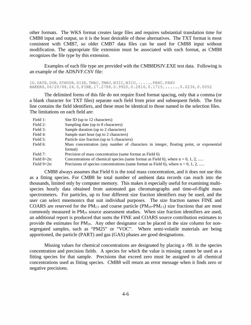
Examples of each file type are provided with the CMB8DSJV.EXE test data. Following isan example of the ADSJVF.CSV file:

ID,DATE,DUR,STHOUR,SIZE,TMAC,TMAU,N3IC,N3IU,.....,PBXC,PBXUBAKERS,06/20/88,24,0,FINE,17.2788,0.9920,0.2816,0.1715,.....,0.0236,0.0052

The delimited forms of this file do not require fixed format spacing, only that a comma (ora blank character for TXT files) separate each field from prior and subsequent fields. The firstline contains the field identifiers, and these must be identical to those named in the selection files. The limitations on each field are:

Field 1: Site ID (up to 12 characters) Field 2: Sampling date (up to 8 characters) Field 3: Sample duration (up to 2 characters) Field 4: Sample start hour (up to 2 characters) Field 5: Particle size fraction (up to 5 characters) Field 6: Mass concentration (any number of characters in integer, floating point, or exponential

format) Field 7: Precision of mass concentration (same format as Field 6) Field 8+2n: Concentrations of chemical species (same format as Field 6), where n = 0, 1, 2, ..... Field 9+2n: Precisions of species concentrations (same format as Field 6), where n = 0, 1, 2, .....

CMB8 always assumes that Field 6 is the total mass concentration, and it does not use thisas a fitting species. For CMB8 he total number of ambient data records can reach into thethousands, limited only by computer memory. This makes it especially useful for examining multi-species hourly data obtained from automated gas chromatographs and time-of-flight massspectrometers. For particles, up to four different size fraction identifiers may be used, and theuser can select mnemonics that suit individual purposes. The size fraction names FINE andCOARS are reserved for the PM2.5 and coarse particle (PM10-PM2.5) size fractions that are mostcommonly measured in PM10 source assessment studies. When size fraction identifiers are used,an additional report is produced that sums the FINE and COARS source contribution estimates toprovide the estimates for PM10. Any other designator can be placed in the size column for non-segregated samples, such as “PM25” or “VOC”. Where semi-volatile materials are beingapportioned, the particle (PART) and gas (GAS) phases are good designations.

Missing values for chemical concentrations are designated by placing a -99. in the speciesconcentration and precision fields. A species for which the value is missing cannot be used as afitting species for that sample. Precisions that exceed zero must be assigned to all chemicalconcentrations used as fitting species. CMB8 will return an error message when it finds zero ornegative precisions.

4-7

4.2.4 Source Profile Input File (PR*.CSV, PR*.DBF, PR*.TXT, PR*.WKS)

Source profile data files may be formatted as column-separated values in ASCII text(CSV), xBASE (DBF), blank-delimited ASCII text (TXT), or Lotus Worksheets (WKS). TheCSV and DBF formats are the most portable and easily prepared. The appropriate file extensionmust be associated with each format, as CMB8 recognizes the file type by this extension.Examples of each file type are provided with the CMB8DSJV.EXE test data. Following is anexample of the PRSJVF.CSV file:PNO,SID,SIZE,N3IC,N3IU,.....,PBXC,PBXUSJV001,SOIL01,FINE,0.002700,0.004700,.......,0.000000,0.000000

The delimited forms of this file do not require fixed format spacing, only that a comma (ora blank character for TXT files) separate each field from prior and subsequent fields. The firstline contains the field identifiers, and these must be identical to those named in the selection files. The limitations on each field are:

Field 1: Profile number or source code (up to six characters)Field 2: Source mnemonic (up to eight characters)Field 3: Particle size fraction (up to five characters)Field 4+2n: Fraction of species in primary mass of source emissions (floating point or exponential format),where n = 0, 1, 2, ...Field 5+2n: Variability of fraction of species in primary mass of source emissions (same format as Field 4),where n = 0, 1, 2, ....

The first record of the profile file contains the species codes for each field. Theseidentifiers can be up to six alphanumeric characters in length, and must correspond to theidentifiers used in the ambient data file. Source profile abundances are expressed in fractions oftotal mass, not in percent. This file does not contain a mass concentration field, as does theambient data file, because all species abundances have been divided by this mass. The totalnumber of records included depends on the number of species, number of sources, and size of thecomputer memory.

From one to four different size fraction identifiers may be used, but these must be thesame as those used in the ambient data and sample selection files. Missing values for chemicalspecies in source profile files can be replaced by a best estimate with a large uncertainty if they areto be used as fitting species, or with –99 if they will not be used. Default values of 0 for thefraction and 0.0001 to 0.01 for the precision are often chosen for species that are expected to bepresent in small abundances. This indicates that the species is present in source emissions at aconcentration less than .01% to 1%. A smaller value may be appropriate for certain source-typesand species. A precision value that exceeds zero must be entered for all fitting species. CMB8will return an error message when it detects precisions that are less than or equal to zero.

4.3 Output Files

Report and data base output files are produced by CMB8.

4-8

4.3.1 Report Output File: RPXXXXRP.TXT

The report output file presents the source contribution estimates, standard errors, modelperformance measures, and measured and calculated chemical concentrations for each sample. The report written to the output file is identical to that which appears in the Output windowduring an interactive modeling session. It is in ASCII text format and can be imported into wordprocessing programs to document the source contributions calculated for each sample. Allinformation needed to independently repeat the source apportionment is contained in this report. Examples of the report are shown in Section 6.

4.3.2 Data Base Output File

The data base output file records the contribution of each source-type to each chemicalspecies in a single data record. Sample identifiers and model performance measures are alsoincluded in each record. This file may be written in blank-delimited (TXT), comma separatedvalues (CSV), xBASE (DBF), or Lotus 123 (WKS) formats (See Sec. 3 ). The file structure is:

Field 1: Species Code Field 2: Species Name Field 3: Fitting flag; a '*' indicates a fitting species, while a '_' indicates a floating species Field 4: Sampling site identifier Field 5: Sampling date Field 6: Sample start hour Field 7: Sample duration Field 8: Particle size fraction Field 9: Measured species concentration Field 10: Precision of measured species concentration Field 11: R square value Field 12: Chi square value Field 13: Percent of measured mass Field 14+2n: Source contribution estimate, n = 0, 1, 2, .... Field 15+2n: Standard error of source contribution estimate, n = 0, 1, 2, ....

Fields 1, 2, and 4 through 10 record the sample information. Fields 3 and 11 through 13provide information about the CMB calculation. The remaining fields correspond to each sourceprofile in the PRXXXXYY file and contain the source contribution estimates and standard errorsfor these sources. A value of -99 is recorded when a profile was not used in the calculation.

The first record in this output file contains the field identifiers. All subsequent recordscontain data. Fields 14+2n and 15+2n are labeled with source codes and source contributionuncertainty columns are labeled with source names.

4.4 Creating Data Input Files

For blank delimited and comma separated value input files, there are three commonmethods of creating CMB8 input files: 1) manually entering the data in the correct format using atext editor or word processing program; 2) editing existing input files with a text editor or wordprocessing program; or 3) transferring files from computerized data bases.

4-9

A text editor or word processor in text mode can be used to type entire input files. It isbest to bring the example files into the editor, then insert the new values in the same locations asthe existing values by using the editor in TYPEOVER mode. Spaces between fields should beentered with the space bar; tabs should not be set. Each line should be terminated with theENTER key rather than using the wraparound feature present in many editors. No blank lines atthe end of the file should be present. Completed files should be saved with an appropriatefilename. The DOS EDIT command is a convenient and commonly available text editor, but itcannot read very long files. Notepad or Wordpad that are included as Windows accessories canalso be used.

When data files have been prepared for other applications (e.g., source profiles may becommon to several different data sets), these files may be cut and pasted to produce the neededinput data files. Owing to differences in individual editing programs, the user is should consult themanual for the editing program to be used for directions on opening a copy of the existing file,deleting and adding material, saving the changes, and renaming the file. When word processors(e.g. Word or Wordperfect), the files must be saved as DOS text with line breaks, otherwise,extra information is included in the files that CMB8 cannot read.

Input files are most easily produced with spreadsheet or data base software. Many sourceprofile and ambient data sets are available in data base management formats. Selections of data,field names, and data structure can be easily made by the data base software. These can be savedusing the Save As or Export selections from the File menu. The CSV, DBF, and WKS formatscan be selected from the “Save as type” option box that usually appears in the “Save As” window.

4.5 Reading Output Files

Report text files can be read directly into a word-processing program (e.g. Word orWordperfect) where the detailed output for each sample can be usually be displayed on a singlepage with columns aligned using the Courier 8-point to 10-point font. A fixed-with font in whichevery character occupies the same space is needed for columns to be correctly aligned. Data baseoutput files can be opened directly by data base or spreadsheet programs that recognize the CSV,DBF, TXT, and WKS extensions. The contents of the CMB8 output window can also beselected and copied to the clipboard for pasting into other Windows programs. Graphs made withCMB8 can be copied to the Windows clipboard with the Clip button, then pasted into a text boxor frame in a word processing program.

5-1

5. USING CMB8

This section illustrates CMB8 commands and operations using the San Joaquin Valley,CA, PM2.5 data set. The other test data sets are provided as examples of additional data base fileformats and for independent practice in CMB8 application and validation. These examples aremost effective when accompanied by actual application of CMB8 on the user’s computer.

5.1 Start CMB8

Start CMB8 by double-clicking on the CMB8 icon in the CMB80 folder, as shown inFigure 5.1.1, or by selecting it from the start menu. CMB8 may also be started from a DOSwindow by typing “CMB8” at the command line.

Figure 5.1.1. Double-click the CMB8.EXE icon to start.

When the “Restart from previous session?” box appears, click No. Clicking Yes willrestore settings and data sets from the previous session. Try this option after completing thisexample.

5.2 Select Data Set

Click Yes when asked to use a CMB8 file names file. Clicking No will initiate a series ofprompts for individual input file names. When the Open window appears, click on theINSJVF.IN8 selection. The default extension for file names files is IN8, and only files with thisextension are listed in the selection box. To view all available files, replace *.IN8 with *.*, andall files in the CMB80 directory will appear in the selection box. The directory may be changedfrom the Look In box if files are located in another folder.

5.3 Examine the CMB8 Banner

Figure 5.3.1 shows the CMB8 banner. The parenthetical number in the second line after

5-2

CMB8 (97350) indicates the latest revision. It consists of the year (97) and julian day(350=12/22) on which CMB8 was most recently revised. It is good practice to verify this againstthe postings on U.S. EPA’s bulletin board to assure that the most recent revision is being used.CMB8 is being continually improved as users respond with recommendations or difficulties. Thedata line underneath the toolbar shows the first ambient sample selected for CMB sourceapportionment, including its site, date, duration, start time, and size fraction. When the Fitindicator reads NO, it means that no calculations have yet been performed for this sample, and nosource contribution estimates can be displayed. This line will always correspond to the currentsample being analyzed.

Figure 5.3.1. CMB8 banner page.

5.4 Set Options

Click on the OPT toolbar button (or select Options from the Main menu, or enter CTRL-T from the keyboard) to bring up the options window. Change the output file format to DBF byclicking the CMBOUTDB.DBF radio button. Change the RP Name to OUSJVFRP.TXT and theDB Name to OUSJVFDB.DBF by entering these over the default names. Change the DisplayDec’s value from 5 to 4, which is accommodates most PM2.5 mass and chemical concentrations

5-3

expressed in µg/m3. A value of 1 or 2 is best for concentrations expressed in ng/m3 or for VOCs

expressed in ppbC or µg/m3. Leave the other options with their default values and click the OKbutton to record these options

Figure 5.4.1. Options window.

5.5 Select Samples

Click on the SAM toolbar button (or enter CTRL-M or click on Select Samples from theMain menu) to select the samples to be apportioned.

5-4

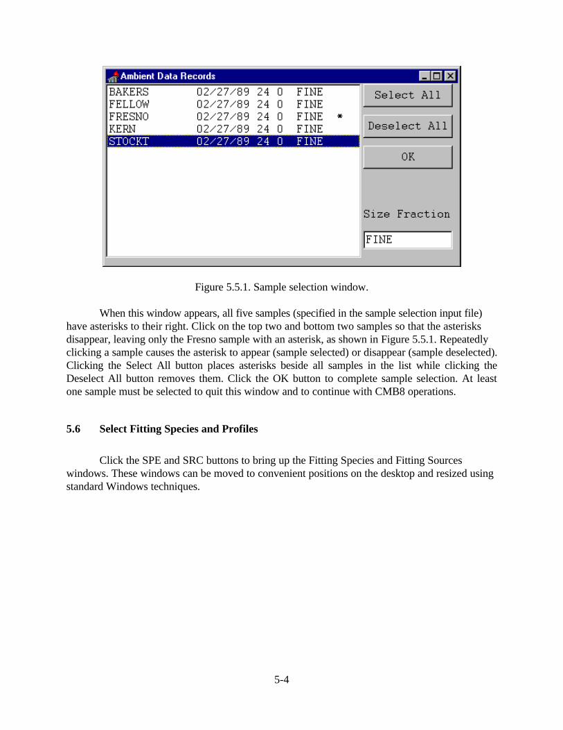
Figure 5.5.1. Sample selection window.

When this window appears, all five samples (specified in the sample selection input file)have asterisks to their right. Click on the top two and bottom two samples so that the asterisksdisappear, leaving only the Fresno sample with an asterisk, as shown in Figure 5.5.1. Repeatedlyclicking a sample causes the asterisk to appear (sample selected) or disappear (sample deselected).Clicking the Select All button places asterisks beside all samples in the list while clicking theDeselect All button removes them. Click the OK button to complete sample selection. At leastone sample must be selected to quit this window and to continue with CMB8 operations.

5.6 Select Fitting Species and Profiles

Click the SPE and SRC buttons to bring up the Fitting Species and Fitting Sourceswindows. These windows can be moved to convenient positions on the desktop and resized usingstandard Windows techniques.

5-5

Figure 5.6.1. Fitting species and fitting source profile windows.

These windows remain open until the x-box in the upper right-hand corner is clicked.Windows can also be minimized using the standard windows techniques. They will return to theiradjusted sizes and positions when the SPE and SRC buttons are pushed. An asterisk next to aspecies or profile mnemonic indicates that this is a fitting species or profile that will be used in theCMB calculation. Clicking on a mnemonic toggles between selection or deselection of thecorresponding species or profile. The Select All and Deselect All buttons are used to place orremove an asterisk beside all mnemonics. The scroll bar to the right of each window is used toview the complete list of selections.

Clicking on the Defaults button in the Fitting Species window opens the Default FittingSpecies window shown in Figure 5.6.2.

5-6

Figure 5.6.2. Default fitting species.

A similar window appears when the Defaults button is clicked in the Fitting Sourceswindow. Up to ten combinations of fitting species and profiles can be defined in this window,with the first one being selected by default. The radio button at the top of the window indicatesthe combination that is currently in effect. The defaults indicated by asterisks in Figure 5.6.2 weredefined in the species selection input file. They can be modified for the current CMB session byclicking the Modify button, then clicking in the appropriate box to toggle between selection anddeselection. Only four combinations are illustrated in Figure 5.6.2, and six additional combinationsmay be entered into the blank columns to the right. These defaults combinations are convenientwhen CMB calculations are performed on samples from several locations or duringdifferent timesof the year that have different contributors. They are also used by the Autofit option to iterateamong different source combinations until the weighted Fit Measure is optimized. Click on OK tofinalize the selection.

5.7 Perform CMB Calculation and Review Results

Click the FIT button and the output window displays the CMB output and performancemeasures. These are discussed in Section 6. In the fitting species window, select Defaults andclick the third radio button that corresponds to a set of profiles more appropriate for Fresno insamples, click OK, then click the FIT button again. The source contribution report is illustratedin Figure 5.7.1. Scroll through the output to examine the most recent source contributions shownin Figure 5.7.1.

5-7

Figure 5.7.1. Output window with CMB source contribution estimates.

CMB outputs from both fits appear in the window, with the most recent output using theFresno profile selection printed below the first apportionment with the default profiles. Click theClear Last button and the most recent output disappears while retaining the previous output.Click the Clear button and all output displayed in the Output window disappears. Notice that theFit indicator on the menu bar changed from NO to YES after the FIT button was clicked the firsttime.

Click the SHO button to recall the most recent calculation, then click the Write Last andWrite DB buttons to record these results in the CMB8 output files. Experiment with the Printand Print Last buttons to obtain a hardcopy of calculation results from the Output window.

5.8 Examine Performance Measures

CMB performance diagnostics are described in Section 6. Most of these appear with thesource contribution estimates in the Output window. The source contributions to species areobtained by clicking the SCN button to provide the output shown in Figure 5.8.1. This shows thefraction of each ambient chemical concentration contributed by each profile. In this example, it isapparent that the SOIL03 profile substantially overestimates aluminum and silicon concentrations.

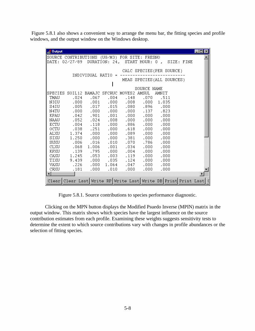
5-8

Figure 5.8.1 also shows a convenient way to arrange the menu bar, the fitting species and profilewindows, and the output window on the Windows desktop.

Figure 5.8.1. Source contributions to species performance diagnostic.

Clicking on the MPN button displays the Modified Psuedo Inverse (MPIN) matrix in theoutput window. This matrix shows which species have the largest influence on the sourcecontribution estimates from each profile. Examining these weights suggests sensitivity tests todetermine the extent to which source contributions vary with changes in profile abundances or theselection of fitting species.

5-9

Figure 5.8.2. MPIN matrix in the Output window.

These displays can be written to the report profile by clicking on the Write Last or WriteRP buttons, or they can sent to the printer with the Print or Print Last buttons.

5.9 Autofit

The Autofit option calculates source contributions for all selected samples without having to examine each one. Click on the AUT button, then click on Yes in the confirmation box. Whenthe sample selection box appears, click on Select All, then on the OK button. Watch the statusline below the CMB8 toolbar change as the source contribution estimates are calculated for eachof the selected samples. Data are written to the RP and DB output files as part of the Autofitprocedure so that they can be examined later.

5.10 Examine Source Profiles and Receptor Concentrations

Click on the PRO button and all source profile chemical abundances are listed in theOutput window, as shown in Figure 5.10.1. This is a good way to verify that data have beencorrectly read from the input files and to determine which species are most abundant in eachprofile. The top number in each species row contains the fractional mass abundance and thesecond row contains the uncertainty of that abundance.

5-10

Figure 5.10.1. Source profile listing.

Clicking on the RCN button writes the receptor concentrations for the current sample tothe Output window. This display can also be used to verify input data.

5.11 Graph Source Profiles, Ambient Concentrations, and Source Contributions

Select Species from the Graph menu, and a display similar to Figure 5.11.1 appears. Theheight of the bar shows the calculated concentration, the horizontal line shows the measuredconcentration, and the error bar shows the precision of the receptor measurements.

5-11

Figure 5.11.1. Example of Species selection from the Graph menu.

Try the same for the Source Profiles option in the Graph menu. In this case a selectionbox appears from which the desired source may be marked by clicking on its mnemonic, thengraphed when the OK button is clicked. Click on the Source Contributions option in the Graphmenu to create a pie plot of source contributions for the current sample. Experiment with theClip, Print, and Orient buttons as described in Section 3. In particular, Clip one of the graphs andpaste it into another Windows program such as Microsoft Word.

5.12 Plot Spatial Pies

After Autofit has been executed and source contribution estimates are available for allsites, select the Spatial Pies option from the Graph menu. Click the OK button when asked toselect sites. Sites are selected by depressing the CTRL key while clicking on the desired sites.Click the OK button to create a spatial display similar to that of Figure 5.12.1.

5-12

5.13 Exit CMB8

From the Files menu, click the Exit button to close CMB8.

Figure 5.13.1. Example of a spatial pie plot of CMB source contributions.

5.14 Working with Large Amounts of Data

Open the INSJVF.IN8 file in a text editor (e.g. DOS edit or Windows Notepad), replacethe third line containing DSSJVF.SEL with XXXXX, and save the modified file as INSJVF1.IN8. Start CMB8 and select Yes to restart from previous session. Open the INSJVF1.IN8 input filefrom the File menu. This preserves previously selected options and window placement.

Examine the Ambient Data Records window with the SAM button. All available samplesin the data input file are now available for examinations. Select all of the samples and performAutofit. If a window such as that illustrated in Figure 5.14.1 appears, the source contributionsfor that sample have not converged after 20 iterations. Select Continue with iteration delta=20several times to determine whether or not convergence can be achieved with a few more

5-13

iterations. The maximum number of iterations can be changed in the options menu by selectingContinue. Change iteration delta. If no convergence can be achieved, there is probably excessivecollinearity for this sample that must be treated individually. Note the sampling site, date, andtime, then select Exit without viewing results to continue with Autofit.

To plot a time series of source contributions, select Time Series from the Graph menu,select one of the sites from the site list menu that appears, and click OK. Select the dates to beplotted from the sample menu that appears by scrolling or clicking with the mouse whiledepressing the CTRL key. No more than 25 samples may be selected for an individual time seriesplot. Click OK, and a stacked bar plot similar to that in Figure 5.14.2 results.

Figure 5.14.1. Options that appear when a CMB calculation does not converge.

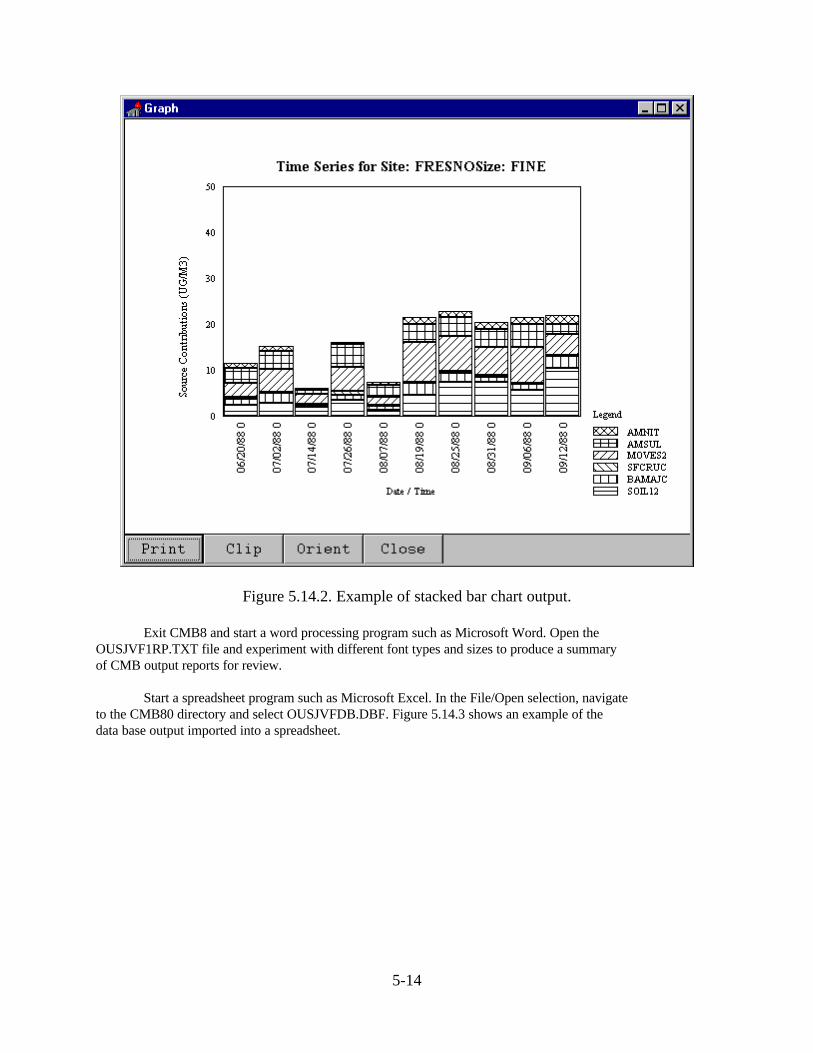
5-14

Figure 5.14.2. Example of stacked bar chart output.

Exit CMB8 and start a word processing program such as Microsoft Word. Open theOUSJVF1RP.TXT file and experiment with different font types and sizes to produce a summaryof CMB output reports for review.

Start a spreadsheet program such as Microsoft Excel. In the File/Open selection, navigateto the CMB80 directory and select OUSJVFDB.DBF. Figure 5.14.3 shows an example of thedata base output imported into a spreadsheet.

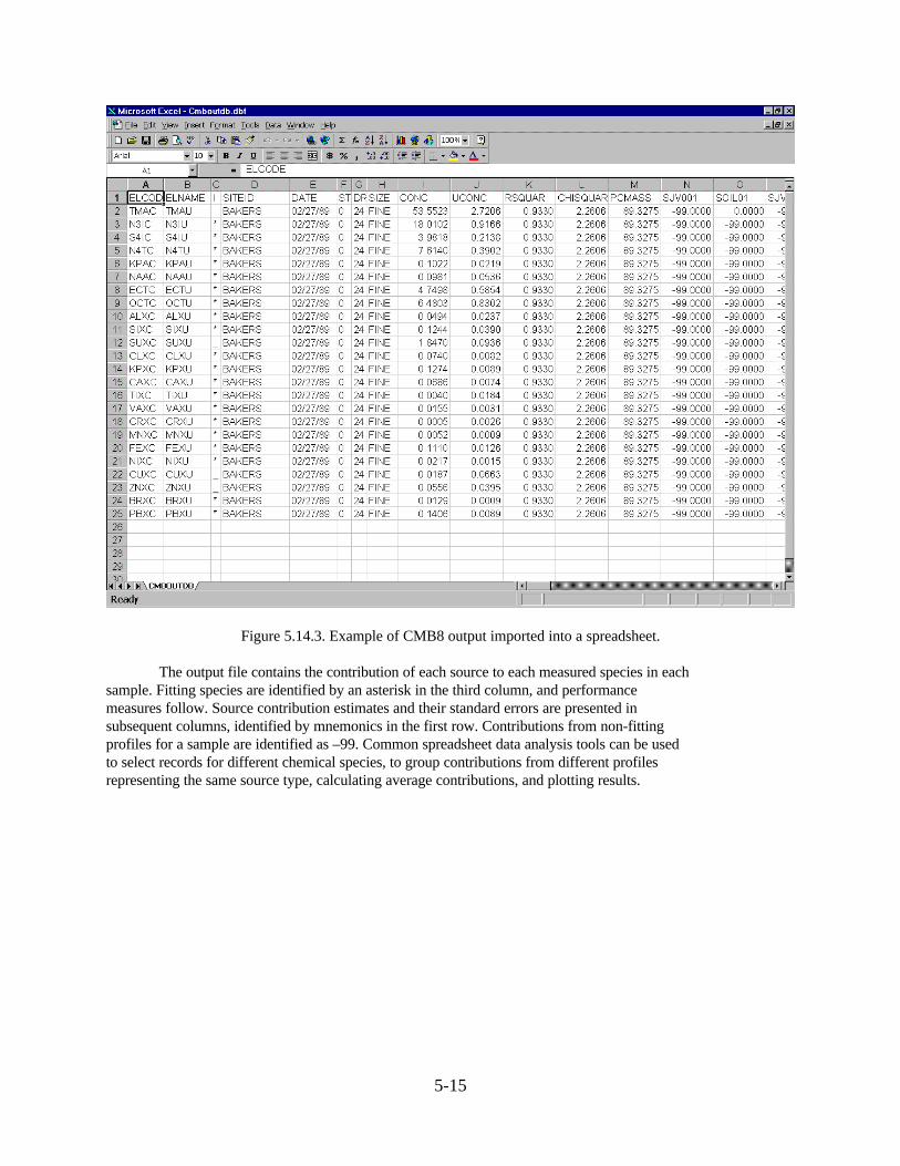
5-15

Figure 5.14.3. Example of CMB8 output imported into a spreadsheet.

The output file contains the contribution of each source to each measured species in eachsample. Fitting species are identified by an asterisk in the third column, and performancemeasures follow. Source contribution estimates and their standard errors are presented insubsequent columns, identified by mnemonics in the first row. Contributions from non-fittingprofiles for a sample are identified as –99. Common spreadsheet data analysis tools can be usedto select records for different chemical species, to group contributions from different profilesrepresenting the same source type, calculating average contributions, and plotting results.

6-1

6. CMB PERFORMANCE MEASURES

This section describes the different performance measures that are used to evaluate thevalidity of source contribution estimates. Greater detail on the use of the performance measuresis presented by Watson et al. (1998). The performance measures are presented in three separatedisplays when the Calculate Source Contributions or Show Fit menu options are invoked: 1) thesource contribution display; 2) the eligible space display; and 3) the species concentration display. Each of these displays is discussed below.

6.1 Source Contribution Estimates Display

An example of a source contribution table display is shown below:SOURCE CONTRIBUTION ESTIMATES - SITE: FRESNO DATE: 02/27/89 CMB8 (97350)SAMPLE DURATION 24 START HOUR 0 SIZE: FINE R SQUARE .96 PERCENT MASS 83.2 CHI SQUARE 1.06 DF 13 B and L: No SRC ELIM: NoWEIGHTS: CHISQR 1.000 R SQR 1.000 PCMASS 1.000 FRCEST 1.000 SOURCE EST CODE NAME SCE(UG/M3) STD ERR TSTAT ---------------------------------------------------- YES SJV002 SOIL03 1.2276 .1588 7.7281 YES SJV017 BAMAJC 3.4511 .7703 4.4800 YES SJV027 SFCRUC .2043 .1290 1.5834 YES SJV036 MOVES2 7.3898 1.8264 4.0461 YES SJV051 AMSUL 3.5726 .5566 6.4184 YES SJV054 AMNIT 25.3561 2.1106 12.0137 YES SJV056 NANO3 .6795 .3511 1.9354 ---------------------------------------------------- MEASURED CONCENTRATION FOR SIZE: FINE 50.3+- 2.6

Source contribution estimates are the main output of the CMB model. The sum of theseconcentrations approximates the total mass concentration. Negative source contributionestimates are not physically meaningful, but they can occur when a source profile is collinear withanother profile or when the source contribution is close to zero. Collinearity is usually identifiedin the eligible sources display. When the absolute value of a positive or negative sourcecontribution estimate is less than its standard error, the source contribution is undetectable. Twoor three times the standard error may be taken as an upper limit of the source contribution in thiscase.

The standard errors reflect the precisions of the ambient data, the source profiles, and theamount of collinearity among different profiles. Standard errors should be reported with everysource contribution estimate. The standard error is a single standard deviation. There is about a66% probability that the true source contribution is within one standard error and about a 95%probability that the true contribution is within two standard errors of the source contributionestimate.

The T-statistic (TSTAT) is the ratio of the source contribution estimate to the standarderror. A TSTAT value less than 2.0 indicates that the source contribution estimate is at or below

6-2

a detection limit. Low TSTAT values for several source contributions may be caused bycollinearities among their profiles; this will be indicated by the Similarity/Uncertainty Clusters.

The reduced chi square, degrees of freedom, R square, percent mass, and fit measure areperformance measures for the least squares calculation.

The chi-square is the weighted sum of squares of the differences between the calculatedand measured fitting species concentrations. The weighting is inversely proportional to thesquares of the precisions in the source profiles and ambient data for each species. Ideally, therewould be no difference between calculated and measured species concentrations and chi-squarewould equal zero. A value less than 1 indicates a very good fit to the data, while values between1 and 2 are acceptable. Chi-square values greater than 4 indicate that one or more speciesconcentrations are not well explained by the source contribution estimates. The degrees offreedom equal the number of fitting species minus the number of fitting sources. The degrees offreedom is needed when statistical significance tests are applied to the chi-square value.

The R-square is the fraction of the variance in the measured concentrations that isexplained by the variance in the calculated species concentrations. It is determined by a linearregression of measured versus model-calculated values for the fitting species. R-square rangesfrom 0 to 1.0. The closer the value is to 1.0, the better the source contribution estimates explainthe measured concentrations. When R-square is less than 0.8, the source contribution estimatesdo not explain the observations very well with the fitting source profiles and/or species.

Percent mass is the percent ratio of the sum of the model-calculated source contributionestimates to the measured mass concentration. This ratio should equal 100%, although valuesranging from 80 to 120% are acceptable. If the measured mass is very low (< 5 to 10 µg/m3),percent mass may be outside of this range because the precision of the mass measurement is onthe order of 1 to 2 µg/m3.

The Fit Measure is calculated using the algorithm

Fit_measure = Wt_chisqr * ( 2 / chisqr )

+ Wt_R-square *R-square

+ Wt_pcmass * pcmass / 100 (for pcmass < 100) or + Wt_pcmass * 100 / pcmass ( for pcmass > 100)

+ Wt_fracest * Frac_Est

where chisqr, rsquare, and pcmass are the performance measures for reduced chi-square, R-square, and per cent mass, respectively, and where Frac_Est is the ratio of the number ofestimable fitting sources to the total number of fitting sources. The weights accorded to each ofthese variables (Wt_chisqr, Wt_R-square, Wt_pcmass , and Wt_fracest) are set to 1.0 by default. These weights may be changed in the Options window.

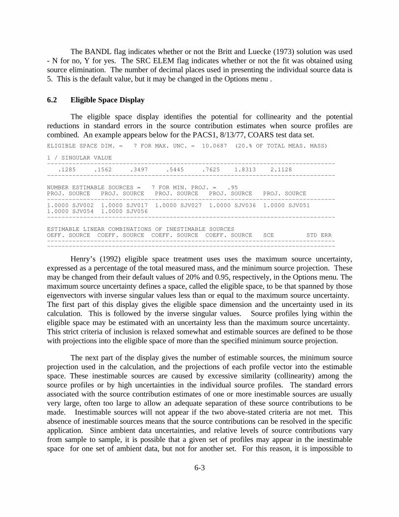
6-3

The BANDL flag indicates whether or not the Britt and Luecke (1973) solution was used- N for no, Y for yes. The SRC ELEM flag indicates whether or not the fit was obtained usingsource elimination. The number of decimal places used in presenting the individual source data is5. This is the default value, but it may be changed in the Options menu .

6.2 Eligible Space Display

The eligible space display identifies the potential for collinearity and the potentialreductions in standard errors in the source contribution estimates when source profiles arecombined. An example appears below for the PACS1, 8/13/77, COARS test data set.ELIGIBLE SPACE DIM. = 7 FOR MAX. UNC. = 10.0687 (20.% OF TOTAL MEAS. MASS)

1 / SINGULAR VALUE -------------------------------------------------------------------------------- .1285 .1562 .3497 .5445 .7625 1.8313 2.1128 -------------------------------------------------------------------------------- NUMBER ESTIMABLE SOURCES = 7 FOR MIN. PROJ. = .95 PROJ. SOURCE PROJ. SOURCE PROJ. SOURCE PROJ. SOURCE PROJ. SOURCE --------------------------------------------------------------------------------1.0000 SJV002 1.0000 SJV017 1.0000 SJV027 1.0000 SJV036 1.0000 SJV051 1.0000 SJV054 1.0000 SJV056 -------------------------------------------------------------------------------- ESTIMABLE LINEAR COMBINATIONS OF INESTIMABLE SOURCES OEFF. SOURCE COEFF. SOURCE COEFF. SOURCE COEFF. SOURCE SCE STD ERR----------------------------------------------------------------------------------------------------------------------------------------------------------------

Henry’s (1992) eligible space treatment uses uses the maximum source uncertainty,expressed as a percentage of the total measured mass, and the minimum source projection. Thesemay be changed from their default values of 20% and 0.95, respectively, in the Options menu. Themaximum source uncertainty defines a space, called the eligible space, to be that spanned by thoseeigenvectors with inverse singular values less than or equal to the maximum source uncertainty. The first part of this display gives the eligible space dimension and the uncertainty used in itscalculation. This is followed by the inverse singular values. Source profiles lying within theeligible space may be estimated with an uncertainty less than the maximum source uncertainty. This strict criteria of inclusion is relaxed somewhat and estimable sources are defined to be thosewith projections into the eligible space of more than the specified minimum source projection.

The next part of the display gives the number of estimable sources, the minimum sourceprojection used in the calculation, and the projections of each profile vector into the estimablespace. These inestimable sources are caused by excessive similarity (collinearity) among thesource profiles or by high uncertainties in the individual source profiles. The standard errorsassociated with the source contribution estimates of one or more inestimable sources are usuallyvery large, often too large to allow an adequate separation of these source contributions to bemade. Inestimable sources will not appear if the two above-stated criteria are not met. Thisabsence of inestimable sources means that the source contributions can be resolved in the specificapplication. Since ambient data uncertainties, and relative levels of source contributions varyfrom sample to sample, it is possible that a given set of profiles may appear in the inestimablespace for one set of ambient data, but not for another set. For this reason, it is impossible to

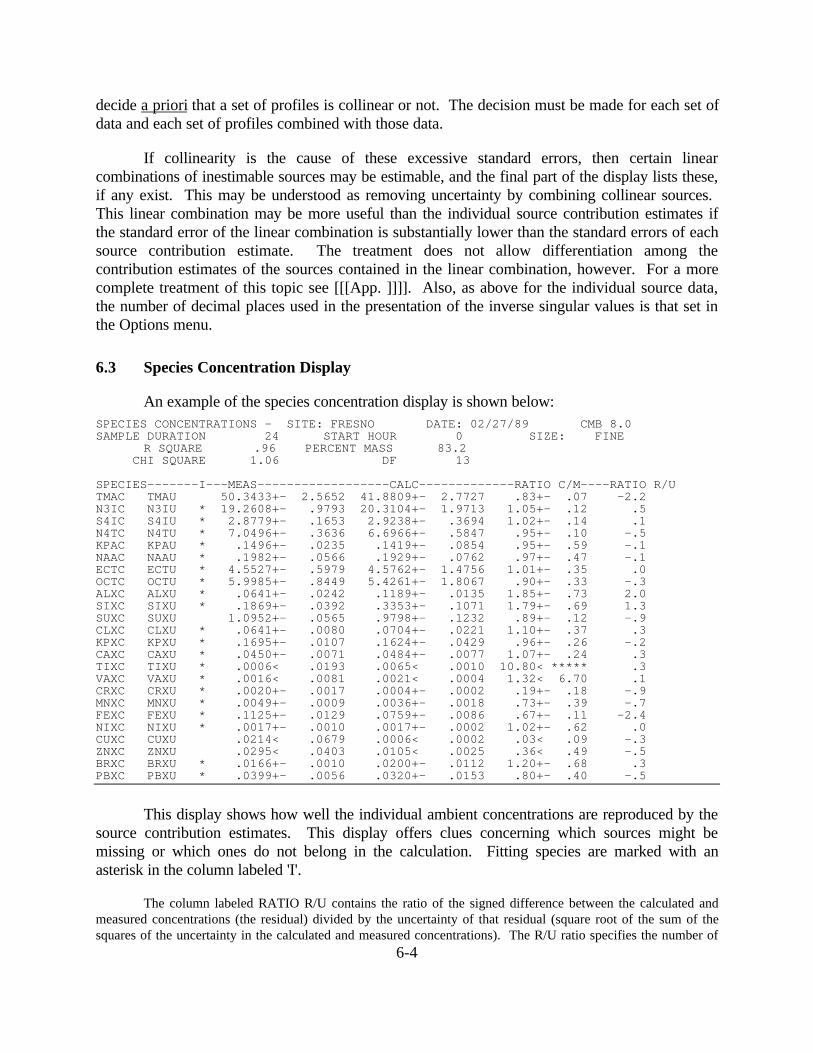
6-4

decide a priori that a set of profiles is collinear or not. The decision must be made for each set ofdata and each set of profiles combined with those data.

If collinearity is the cause of these excessive standard errors, then certain linearcombinations of inestimable sources may be estimable, and the final part of the display lists these,if any exist. This may be understood as removing uncertainty by combining collinear sources. This linear combination may be more useful than the individual source contribution estimates ifthe standard error of the linear combination is substantially lower than the standard errors of eachsource contribution estimate. The treatment does not allow differentiation among thecontribution estimates of the sources contained in the linear combination, however. For a morecomplete treatment of this topic see [[[App. ]]]]. Also, as above for the individual source data,the number of decimal places used in the presentation of the inverse singular values is that set inthe Options menu.

6.3 Species Concentration Display

An example of the species concentration display is shown below:SPECIES CONCENTRATIONS - SITE: FRESNO DATE: 02/27/89 CMB 8.0SAMPLE DURATION 24 START HOUR 0 SIZE: FINE

R SQUARE .96 PERCENT MASS 83.2 CHI SQUARE 1.06 DF 13

SPECIES-------I---MEAS------------------CALC-------------RATIO C/M----RATIO R/UTMAC TMAU 50.3433+- 2.5652 41.8809+- 2.7727 .83+- .07 -2.2 N3IC N3IU * 19.2608+- .9793 20.3104+- 1.9713 1.05+- .12 .5 S4IC S4IU * 2.8779+- .1653 2.9238+- .3694 1.02+- .14 .1 N4TC N4TU * 7.0496+- .3636 6.6966+- .5847 .95+- .10 -.5 KPAC KPAU * .1496+- .0235 .1419+- .0854 .95+- .59 -.1 NAAC NAAU * .1982+- .0566 .1929+- .0762 .97+- .47 -.1 ECTC ECTU * 4.5527+- .5979 4.5762+- 1.4756 1.01+- .35 .0 OCTC OCTU * 5.9985+- .8449 5.4261+- 1.8067 .90+- .33 -.3 ALXC ALXU * .0641+- .0242 .1189+- .0135 1.85+- .73 2.0 SIXC SIXU * .1869+- .0392 .3353+- .1071 1.79+- .69 1.3 SUXC SUXU 1.0952+- .0565 .9798+- .1232 .89+- .12 -.9 CLXC CLXU * .0641+- .0080 .0704+- .0221 1.10+- .37 .3 KPXC KPXU * .1695+- .0107 .1624+- .0429 .96+- .26 -.2 CAXC CAXU * .0450+- .0071 .0484+- .0077 1.07+- .24 .3 TIXC TIXU * .0006< .0193 .0065< .0010 10.80< ***** .3 VAXC VAXU * .0016< .0081 .0021< .0004 1.32< 6.70 .1 CRXC CRXU * .0020+- .0017 .0004+- .0002 .19+- .18 -.9 MNXC MNXU * .0049+- .0009 .0036+- .0018 .73+- .39 -.7 FEXC FEXU * .1125+- .0129 .0759+- .0086 .67+- .11 -2.4 NIXC NIXU * .0017+- .0010 .0017+- .0002 1.02+- .62 .0 CUXC CUXU .0214< .0679 .0006< .0002 .03< .09 -.3 ZNXC ZNXU .0295< .0403 .0105< .0025 .36< .49 -.5 BRXC BRXU * .0166+- .0010 .0200+- .0112 1.20+- .68 .3 PBXC PBXU * .0399+- .0056 .0320+- .0153 .80+- .40 -.5

This display shows how well the individual ambient concentrations are reproduced by thesource contribution estimates. This display offers clues concerning which sources might bemissing or which ones do not belong in the calculation. Fitting species are marked with anasterisk in the column labeled 'I'.

The column labeled RATIO R/U contains the ratio of the signed difference between the calculated andmeasured concentrations (the residual) divided by the uncertainty of that residual (square root of the sum of thesquares of the uncertainty in the calculated and measured concentrations). The R/U ratio specifies the number of

6-5

uncertainty intervals by which the calculated and measured concentrations differ. When the absolute value of theR/U ratio exceeds 2, the residual is significant. If it is positive, then one or more of the profiles is contributing toomuch to that species. If it is negative, then there is an insufficient contribution to that species and a source may bemissing. The sum of the squared R/U for fitting species divided by the degrees of freedom yields the chi square. The highest R/U values for fitting species are the cause of high chi square values. Also, as above for theindividual source data, the number of decimal places used in the presentation of the species data isthat set in the Options menu.

6.4 Additional Performance Measures

Main menu choice Present Source Contributions produces a table that shows the fractionof each species' calculated ambient concentration contributed by each source in the fit. Thesources that are major contributors to each species can be determined by examining this display. An example of this display is shown below:SOURCE CONTRIBUTIONS (UG/M3) FOR SITE: FRESNODATE: 02/27/89 DURATION: 24, START HOUR: 0 , SIZE: FINE

CALC SPECIES(PER SOURCE) INDIVIDUAL RATIO = -------------------------- MEAS SPECIES(ALL SOURCES) SOURCE NAMESPECIES SOIL03 BAMAJC SFCRUC MOVES2 AMSUL AMNIT NANO3 TMAU .024 .069 .004 .147 .071 .504 .013 N3IU .000 .001 .000 .008 .000 1.020 .026 S4IU .002 .017 .014 .080 .902 .000 .000 N4TU .000 .000 .000 .000 .138 .811 .000 KPAU .027 .920 .001 .000 .000 .000 .000 NAAU .014 .024 .008 .000 .000 .000 .927 ECTU .006 .120 .000 .879 .000 .000 .000 OCTU .034 .257 .000 .614 .000 .000 .000 ALXU 1.766 .000 .000 .089 .000 .000 .000 SIXU 1.415 .000 .000 .378 .000 .000 .000 SUXU .006 .016 .010 .070 .792 .000 .000 CLXU .036 1.028 .001 .033 .000 .000 .000 KPXU .142 .812 .000 .003 .000 .000 .000 CAXU .900 .054 .003 .118 .000 .000 .000 TIXU 10.639 .000 .034 .123 .000 .000 .000 VAXU .230 .000 1.047 .046 .000 .000 .000 CRXU .184 .000 .010 .000 .000 .000 .000 MNXU .301 .000 .004 .422 .000 .000 .000 FEXU .670 .000 .004 .001 .000 .000 .000 NIXU .072 .000 .949 .000 .000 .000 .000 CUXU .011 .000 .000 .017 .000 .000 .000 ZNXU .100 .105 .018 .133 .000 .000 .000 BRXU .007 .021 .000 1.175 .000 .000 .000 PBXU .111 .000 .000 .691 .000 .000 .000

Another diagnostic is the transpose of the normalized modified pseudo-inverse matrix(MPIN). This matrix indicates the degree of influence each species concentration has on thecontribution and standard of error of the corresponding source category. MPIN is normalizedsuch that it takes on values from -1 to 1. Species with MPIN absolute values of 1 to 0.5 areassociated with influential species. Noninfluential species have MPIN absolute values of 0.3 orless. Species with absolute values between 0.3 and 0.5 are ambiguous but should generally beconsidered noninfluential.

An example display of this diagnostic is shown below:

6-6

TRANSPOSE OF SENSITIVITY MATRIX FOR SITE: FRESNODATE: 02/27/89 DURATION: 24, START HOUR: 0 , SIZE: FINE

SOURCE NAME SPECIES SOIL03 BAMAJC SFCRUC MOVES2 AMSUL AMNIT NANO3 N3IU -.01 .00 .01 .04 -.11 1.00 .05 S4IU .00 .00 .00 .01 1.00 -.20 .01 N4TU .01 .00 -.01 -.04 .12 .90 -.06 KPAU -.02 .50 .00 -.08 .00 .00 .00 NAAU .00 .00 .00 .00 .01 -.12 1.00 ECTU -.17 -.01 .00 1.00 -.08 .01 .00 OCTU -.11 .16 .00 .71 -.06 .01 .00 ALXU .83 -.06 -.02 -.06 .01 .00 .00 SIXU .43 -.06 -.01 .17 -.01 .00 .00 CLXU -.05 .90 .00 -.10 -.01 .00 -.01 KPXU .04 1.00 .00 -.17 .00 .00 -.01 CAXU .76 .01 -.01 .06 -.01 .00 .00 TIXU .07 .00 .00 -.01 .00 .00 .00 VAXU .00 .00 .13 .00 -.01 .00 .00 CRXU .04 .00 .01 -.01 .00 .00 .00 MNXU .08 -.06 .00 .39 -.03 .00 .00 FEXU 1.00 -.06 .00 -.17 .01 .00 .00 NIXU -.02 .00 1.00 .00 -.06 .01 -.01 BRXU -.11 -.07 .00 .70 -.06 .00 .00 PBXU -.05 -.08 .00 .68 -.06 .00 .00

7-1

7. REFERENCES

Barth, D. (1970). Federal motor vehicle emissions goals for CO, HC, and NOx based on desiredair quality levels. JAPCA 20:519.

Britt, H.I. and Luecke, R.H. (1973). The estimation of parameters in nonlinear, implicit models.Technometrics 15:233.

Cass, G.R. and McRae, G.J. (1981). Minimizing the cost of air pollution control.Environ.Sci.Technol. 15:748-57.

Chang, T.Y. and Weinstock, B. (1975). Generalized rollback modeling for urban air pollutioncontrol. JAPCA 25:1033-7.

Chow, J.C., Watson, J.G., Lowenthal, D.H., Pritchett, L.C., Richards, L.W. (1990). San JoaquinValley Air Quality Study, Phase 2: PM10 modeling and analysis, Volume I: Receptor modelingsource apportionment, Final report. Report No. DRI 8929.1F prepared by Desert ResearchInstitute, Reno, NV.

Chow, J.C., Watson, J.G., Lowenthal, D.H., Solomon, P.A., Magliano, K.L., Ziman, S.D.,Richards, L.W. (1992). PM10 source apportionment in California's San Joaquin Valley. Atmos.Environ. 26A:3335-54.

Chow, J.C., Watson, J.G., Ono, D.M., Mathai, C.V. (1993). PM10 standards and nontraditionalparticulate source controls: A summary of the A&WMA/EPA international specialty conference.JAWMA 43:74-84.

Cooper, J.A. and Watson, J.G. (1980). Receptor oriented methods of air particulate sourceapportionment. JAPCA 30:1116-25.

Currie, L.A., Gerlach, R.W., Lewis, C.W., Balfour, W.D., Cooper, J.A., Dattner, S.L., deCesar,R.T., Gordon, G.E., Heisler, S.L., Hopke, P.K., Shah, J.J., Thurston, G.D., Williamson, H.J.(1984). Interlaboratory comparison of source apportionment procedures: Results for simulateddata sets. Atmos. Environ. 18:1517.

deCesar, R.T., Edgerton, S.A., Khalil, M.A.K., Rasmussen, R.A. (1985). Sensitivity analysis ofmass balance receptor modeling: methyl chloride as an indicator of wood smoke. Chemosphere14:1495-501.

deCesar, R.T., Edgerton, S.A., Khalil, M.A.K., Rasmussen, R.A. (1986). A tool for designingreceptor model studies to apportion source impacts with specified precisions. In Transactions,Receptor Methods for Source Apportionment: Real World Issues and Applications, Pace, T.G.editor. Air Pollution Control Association, Pittsburgh, PA. p. 56-67.

deNevers, N. and Morris, J.R. (1975). Rollback modeling: basic and modified. JAPCA 25:943.

7-2

Dzubay, T.G., Stevens, R.K., Balfour, W.D., Williamson, H.J., Cooper, J.A., Core, J.E., deCesar,R.T., Crutcher, E.R., Dattner, S.L., Davis, B.L., Heisler, S.L., Shah, J.J., Hopke, P.K., Johnson,D.L. (1984). Interlaboratory comparison of receptor model results for Houston aerosol. Atmos.Environ. 18:1555.

Friedlander, S.K. (1973). Chemical element balances and identification of air pollution sources.Environ.Sci.Technol. 7:235-40.

Friedlander, S.K. (1981). New developments in receptor modeling theory. In AtmosphericAerosol: Source/Air Quality Relationships, Macias, E.S. and Hopke, P.K. editors. AmericanChemical Society, Washington, DC. p. 1-19.

Fujita, E.M., Watson, J.G., Chow, J.C., Lu, Z. (1994). Validation of the chemical mass balancereceptor model applied to hydrocarbon source apportionment in the Southern California AirQuality Study. Environ.Sci.Technol. 28:1633-49.

Fujita, E.M., Lu, Z., Sagebiel, J.C., Watson, J.G. (1995). Apportionment for the Coastal OxidantAssessment for Southeast Texas. prepared by Desert Research Institute, Reno, NV.

Fujita, E.M., Lu, Z., Sheetz, L., Harshfield, G., Zielinska, B. (1997). Determination of mobilesource emission source fraction using ambient field measurements. prepared by Desert ResearchInstitute, Reno, NV.

Gartrell, G. and Friedlander, S.K. (1975). Relating particulate pollution to sources: The 1972California Aerosol Characterization Study. Atmos. Environ. 9:279-99.

Gordon, G.E. (1980). Receptor models. Environ.Sci.Technol. 14:792-800.

Gordon, G.E. (1988). Receptor models. Environ.Sci.Technol. 22:1132-1142.

Gordon, G.E., Zoller, W.H., Kowalczyk, G.S., Rheingrover, S.W. (1981). Composition of sourcecomponents needed for aerosol receptor models. In Atmospheric Aerosol: Source Air/QualityRelationships, Macias, E.S. and Hopke, P.K. editors. American Chemical Society, Washington,D.C. p. 51-74.

Henry, R.C. (1982). Stability analysis of receptor models that use least squares fitting. InReceptor Models Applied to Contemporary Air Pollution Problems, Hopke, P.K. and Dattner,S.L. editors. Air Pollution Control Association, Pittsburgh, PA. p. 141-62.

Henry, R.C. (1992). Dealing with near collinearity in chemical mass balance receptor models.Atmos. Environ. 26A:933-8.

Hidy, G.M. and Friedlander, S.K. (1972). The nature of the Los Angeles aerosol. In SecondInternational Clean Air Congress, Washington, DC.

7-3

Hidy, G.M. and Venkataraman, C. (1996). The chemical mass balance method for estimatingatmospheric particle sources in Southern California. Chem.Eng.Comm. 151:187-209.

Hopke, P.K. (1985). Receptor Modeling in Environmental Chemistry. John Wiley & Sons, NewYork, NY.

Hopke, P.K. (1991). Receptor Modeling for Air Quality Management. Elsevier Press,Amsterdam, The Netherlands.

Hopke, P.K., Dattner, S.L. (1982). Receptor Models Applied to Contemporary PollutionProblems. Air & Waste Management Association, Pittsburgh, PA.

Hougland, E.S. (1983). Chemical element balance by linear programming. 73rd Annual Meetingof the Air Pollution Control Association, Atlanta, GA.

Javitz, H.S. and Watson, J.G. (1986). Methods of receptor model evaluation and validation. InTransactions, Methods for Source Apportionment: Real World Issues and Applications, Pace,T.G. editor. Air Pollution Control Association, Pittsburgh, PA.

Javitz, H.S., Watson, J.G., Guertin, J.P., Mueller, P.K. (1988a). Results of a receptor modelingfeasibility study. JAPCA 38:661.

Javitz, H.S., Watson, J.G., Robinson, N.F. (1988b). Performance of the chemical mass balancemodel with simulated local-scale aerosols. Atmos. Environ. 22:2309-22.

Kneip, T.J., Kleinman, M.T., Eisenbud, M. (1973). Relative contribution of emission sources tothe total airborne particulates in New York City. In Third International Clean Air Congress,Dusseldorf, FRG.

Larson, T.V. and Vong, R.J. (1989). Partial least squares regression methodology: Application tosource receptor modeling. In Transactions, Receptor Models in Air Resources Management,Watson, J.G. editor. Air & Waste Management Association, Pittsburgh, PA. p. 391-403.

Lin, C. and Milford, J.B. (1994). Decay-adjusted chemical mass balance receptor modeling forvolatile organic compounds. Atmos. Environ. 28:3261-76.

Lowenthal, D.H., Hanumara, R.C., Rahn, K.A., Currie, L.A. (1987). Effects of systematic error,estimates and uncertainties in chemical mass balance apportionments: Quail Roost II revisited.Atmos. Environ. 21:501-10.

Lowenthal, D.H. and Rahn, K.A. (1988a). Reproducibility of regional apportionments of pollutionaerosol in the Northeastern United States. Atmos. Environ. 22:1829-33.

7-4

Lowenthal, D.H. and Rahn, K.A. (1988b). Tests of regional elemental tracers of pollutionaerosols. 2. Sensitivity of signatures and apportionments to variations in operating parameters.Atmos. Environ. 22:420-6.

Lowenthal, D.H., Wunschel, K.R., Rahn, K.A. (1988c). Tests of regional elemental tracers ofpollution aerosols. 1. Distinctness of regional signatures, stability during transport, and empiricalvalidation. Environ.Sci.Technol. 22:413-20.

Lowenthal, D.H., Chow, J.C., Watson, J.G., Neuroth, G.R., Robbins, R.B., Shafritz, B.P.,Countess, R.J. (1992). The effects of collinearity on the ability to determine aerosol contributionsfrom diesel- and gasoline-powered vehicles using the chemical mass balance model. Atmos.Environ. 26A:2341-51.

Lowenthal, D.H., Zielinska, B., Chow, J.C., Watson, J.G., Gautam, M., Ferguson, D.H., Neuroth,G.R., Stevens, K.D. (1994). Characterization of heavy-duty diesel vehicle emissions. Atmos.Environ. 28:731-44.

Miller, M.S., Friedlander, S.K., Hidy, G.M. (1972). A chemical element balance for the Pasadenaaerosol. J.Colloid Interface Sci. 39:165-76.

Pace, T.G., Watson, J.G. (1987). Protocol for applying and validating the CMB model. ReportNo. EPA-450/4-86-010 prepared by Office of Air Quality Planning and Standards, U.S.Environmental Protection Agency, Research Triangle Park, NC.

Song, X.H. and Hopke, P.K. (1996). Solving the chemical mass balance problem using anartificial neural network. Environ.Sci.Technol. 30:531

Stevens, R.K. and Pace, T.G. (1984). Review of the mathematical and empirical receptor modelsworkshop (Quail Roost II). Atmos. Environ. 18:1499-506.

U.S.EPA (1987). Receptor model technical series, Volume III (Revised). CMB user's manual(Version 6.0). Report No. EPA-450/4-83-014R prepared by U.S. Environmental ProtectionAgency, Research Triangle Park, NC.

Venkataraman, C. and Friedlander, S.K. (1994). Source resolution of fine particulate polycyclicaromatic hydrocarbons using a receptor model modified for reactivity. JAWMA 44:1103-8.

Vong, R.J., Geladi, P., Wold, S., Esbensen, K. (1988). Source contributions to ambient aerosolcalculated by discriminant partial least squares regression (PLS). J.Chemometrics 2:281-96.

Watson, J.G. (1979). Chemical element balance receptor model methodology for assessing thesources of fine and total particulate matter in Portland, Oregon. Ph.D. Oregon Graduate Center,Beaverton, OR.

Watson, J.G. (1984). Overview of receptor model principles. JAPCA 34:619-23.

7-5

Watson, J.G. and Chow, J.C. (1994). Clear sky visibility as a challenge for society. AnnualRev.Energy Environ. 19:241-66.

Watson, J.G., Chow, J.C, Lu, Z., Fujita, E.M., Lowenthal, D.H., Lawson, D.R. (1994a).Chemical mass balance source apportionment of PM10 during the Southern California Air QualityStudy. Aerosol Sci. Technol. 21:1-36.

Watson, J.G., Chow, J.C., Lurmann, F.W., Misarra, S. (1994b). Ammonium nitrate, nitric acid,and ammonia equilibrium in wintertime Phoenix, Arizona. JAWMA 44:405-12.

Watson, J.G., Chow, J.C., Mathai, C.V. (1989). Receptor models in air resources management: Asummary of the APCA international specialty conference. JAPCA 39:419-26.

Watson, J.G., Chow, J.C., Pace, T.G. (1991). Chemical mass balance. In Receptor Modeling forAir Quality Management, Hopke, P.K. editor. Elsevier Press, New York, NY. p. 83-116.

Watson, J.G., Cooper, J.A., Huntzicker, J.J. (1984). The effective variance weighting for leastsquares calculations applied to the mass balance receptor model. Atmos. Environ. 18:1347-55.

Watson, J.G., Robinson, N.F., Chow, J.C., Henry, R.C., Kim, B.M., Pace, T.G., Meyer, E.L.,Nguyen, Q. (1990). The USEP/DRI chemical mass balance receptor model, CMB 7.0.Environ.Software 5:38-49.

Williamson, H.J., Dubose, D.A. (1983). Receptor model technical series, Volume III: User'smanual for chemical mass balance model. Report No. EPA-450/4-83-014 prepared by U.S.Environmental Proteciton Agency, Research Triangle Park, NC.

Winchester, J.W. and Nifong, G.D. (1971). Water pollution in Lake Michigan by trace elementsfrom aerosol fallout. Water Air and Soil Pollution 1:50-64.