CheckDP: An Automated and Integrated Approach for ProvingDifferential Privacy or Finding Precise Counterexamples

Yuxin Wang, Zeyu Ding, Daniel Kifer, Danfeng ZhangThe Pennsylvania State University

{yxwang,zyding}@psu.edu,{dkifer,zhang}@cse.psu.edu

ABSTRACTWe propose CheckDP, an automated and integrated approach forproving or disproving claims that a mechanism is differentiallyprivate. CheckDP can find counterexamples for mechanisms withsubtle bugs for which prior counterexample generators have failed.Furthermore, it was able to automatically generate proofs for correctmechanisms for which no formal verification was reported before.CheckDP is built on static program analysis, allowing it to be moreefficient and precise in catching infrequent events than samplingbased counterexample generators (which run mechanisms hun-dreds of thousands of times to estimate their output distribution).Moreover, its sound approach also allows automatic verification ofcorrect mechanisms. When evaluated on standard benchmarks andnewer privacy mechanisms, CheckDP generates proofs (for cor-rect mechanisms) and counterexamples (for incorrect mechanisms)within 70 seconds without any false positives or false negatives.

CCS CONCEPTS• Security and privacy→ Logic and verification; • Theory ofcomputation→ Program analysis.

KEYWORDSDifferential privacy; formal verification; counterexample detectionACM Reference Format:Yuxin Wang, Zeyu Ding, Daniel Kifer, Danfeng Zhang. 2020. CheckDP: AnAutomated and Integrated Approach for Proving Differential Privacy orFinding Precise Counterexamples. In Proceedings of the 2020 ACM SIGSACConference on Computer and Communications Security (CCS ’20), November9–13, 2020, Virtual Event, USA. ACM, New York, NY, USA, 20 pages. https://doi.org/10.1145/3372297.3417282

1 INTRODUCTIONDifferential privacy [27] has been adopted in major data sharinginitiatives by organizations such as Google [15, 29], Apple [48],Microsoft [22], Uber [36] and the U.S. Census Bureau [1, 17, 35, 41].It allows these organizations to collect and share data with provablebounds on the information that is leaked about any individual.

Crucial to any differentially private system is the correctness ofprivacy mechanisms, the underlying privacy primitives in larger

Permission to make digital or hard copies of all or part of this work for personal orclassroom use is granted without fee provided that copies are not made or distributedfor profit or commercial advantage and that copies bear this notice and the full citationon the first page. Copyrights for components of this work owned by others than theauthor(s) must be honored. Abstracting with credit is permitted. To copy otherwise, orrepublish, to post on servers or to redistribute to lists, requires prior specific permissionand/or a fee. Request permissions from permissions@acm.org.CCS ’20, November 9–13, 2020, Virtual Event, USA© 2020 Copyright held by the owner/author(s). Publication rights licensed to ACM.ACM ISBN 978-1-4503-7089-9/20/11. . . $15.00https://doi.org/10.1145/3372297.3417282

privacy-preserving algorithms. Manually developing the necessaryrigorous proofs that a mechanism correctly protects privacy is asubtle and error-prone process. For example, detailed explanationsof significant errors in peer-reviewed papers and systems can befound in [21, 40, 42]. Such mistakes have led to research in the ap-plication of formal verification for proving that mechanisms satisfydifferential privacy [3, 5, 7, 9–11, 51, 52]. However, if a mechanismhas a bug making its privacy claim incorrect, these techniques can-not disprove the privacy claims – a counterexample detector mustbe used instead [14, 23, 34]. Finding a counterexample is typicallya two-phase process that (1) first searches an infinitely large spacefor candidate counterexamples and then (2) uses an exact symbolicprobabilistic solver like PSI [33] to verify that the counterexam-ple is indeed valid. The search phase currently presents the mostproblems (i.e., large runtimes or failure to find counterexamples aremost often attributed to the search phase). Earlier search techniqueswere based on sampling (running a mechanism hundreds of thou-sands of times), which made them slow and inherently imprecise:even with enormous amounts of samples, they can still fail if aprivacy-violating section of code is not executed frequently enoughor if the actual privacy cost is slightly higher than the privacy claim.Recently, static program analyses were proposed to accomplishboth goals [4, 30]. However, they either only analyze a non-trivialbut restricted class of programs [4], or rely on heuristic strategieswhose effectiveness on many sutble mechanisms is unclear [30].

In this paper, we present CheckDP, an automated and integratedtool for proving or disproving the correctness of a mechanism thatclaims to be differentially private. Significantly, CheckDP automati-cally finds counterexamples via static analysis, making it unneces-sary to run the mechanism. Like prior work [14], CheckDP still usesPSI [33] at the end. However, replacing sampling-based search withstatic analysis enables CheckDP to find violations in a few seconds,while previous sampling-based methods [14, 23] may fail even afterrunning for hours. Furthermore, sampling-based methods may stillrequire manual setting of some program inputs (e.g., DP-Finder [14]requires additional arguments to be set manually for Sparse VectorTechnique in our evaluation) while CheckDP is fully automated.Furthermore, the integrated approach of CheckDP allows it to effi-ciently analyze a larger class of differentially privacy mechanisms,compared with concurrent work using static analyses [4, 30].

Meanwhile, CheckDP still offers state-of-the-art verification ca-pability compared with existing language-based verifiers and isfurther able to automatically generate proofs for 3 mechanismsfor which no formal verification was reported before. CheckDPtakes the source code of a mechanism along with its claimed levelof privacy and either generates a proof of correctness or a verifi-able counterexample (a pair of related inputs and a feasible output).

CheckDP is built upon a proof technique called randomness align-ment [24, 51, 52], which recasts the task of proving differentialprivacy into one of finding alignments between random variablesused by two related runs of the mechanism. CheckDP uses a novelverify-invalidate loop that alternatively improves tentative proofs(in the form of alignments), which are then used to improve ten-tative counterexamples (and vice versa) until either the tentativeproof has no counterexample, or the tentative counterexample hasno alignment. We evaluated CheckDP on correct/incorrect versionsof existing benchmarks and newly proposed mechanisms. It gener-ated a proof for each correct mechanism within 70 seconds and acounterexample for each incorrect mechanism within 15 seconds.

In summary, this paper makes the following contributions:(1) CheckDP, one of the first automated tools (with concurrent

work [4, 30]) that generates both proofs for correct mechanismsand counterexamples for incorrect mechanisms (Section 2.4).

(2) A syntax-directed translation from the probabilistic mechanismbeing checked to non-probabilistic target code with explicitproof obligations (Section 3).

(3) An alignment template generation algorithm (Section 3.4).(4) A novel verify-invalidate loop that incrementally improves

tentative proofs and counterexamples (Section 4).(5) Case studies and experimental comparisons between CheckDP

and existing tools using correct/incorrect versions of existingbenchmarks and newly proposed mechanisms. For incorrectmechanisms, CheckDP automatically found counterexamples inall cases, even in cases where competing methods [14, 23] failed.For correct mechanisms, CheckDP automatically generatedproofs of privacy, including proofs for 3 mechanisms for whichno formal verification was reported before (Section 5).

2 PRELIMINARIES AND RUNNING EXAMPLE2.1 Differential PrivacyAmong several popular variants of differential privacy [16, 26, 27,43], we focus on pure differential privacy [27]. The goal of differ-ential privacy is to hide the effect of any person’s record on theoutput of an algorithm. This is achieved by considering all pairs ofdatasets 𝐷 and 𝐷 ′ that differ on one record. We call such datasetsadjacent and denote it by 𝐷 ∼ 𝐷 ′. To offer privacy, a differentiallyprivate algorithm injects carefully calibrated random noise dur-ing its computation. Given a pair of datasets (𝐷,𝐷 ′), we call theexecution of an algorithm on 𝐷 the original execution and the ex-ecution on (neighboring) 𝐷 ′ the related execution. Intuitively, wesay a randomized algorithm is differentially private if the outputdistribution of the original execution and its related execution arehard to distinguish for all such dataset pairs:

Definition 1 (Pure Differential Privacy [25]). Let 𝜖 ≥ 0. Aprobabilistic computation 𝑀 : D → O is 𝜖-differentially private iffor every pair of neighboring datasets 𝐷 ∼ 𝐷 ′ ∈ D and every output𝑜 ∈ O, P[𝑀 (𝐷) = 𝑜] ≤ 𝑒𝜖 P[𝑀 (𝐷 ′) = 𝑜] .

Often, a differentially private algorithm𝑀 interacts with a dataset𝐷 through a list of queries 𝑓1, 𝑓2, . . .: it iteratively runs a query 𝑓𝑖on 𝐷 to get an exact answer 𝑞𝑖 , then performs some randomizedcomputation on the set of query answers {𝑞 𝑗 | 𝑗 ≤ 𝑖}. We call thevector (𝑞1, 𝑞2, . . .) along with other data-independent parameters to

𝑀 (e.g., privacy parameter 𝜖) an input to𝑀 . The notion of adjacentdatasets translates into the notion of sensitivity on those queries:

Definition 2 (Global Sensitivity [28]). The global sensitivityof a query 𝑓 is Δ𝑓 = sup𝐷∼𝐷′

��𝑓 (𝐷) − 𝑓 (𝐷 ′)��.

We say two inputs 𝑖𝑛𝑝 = {(𝑞1, 𝑞2, . . .), params} and 𝑖𝑛𝑝 ′ =

{(𝑞′1, 𝑞′2, . . .), params} are adjacentwith respect to the queries 𝑓1, 𝑓2, . . .,

and write 𝑖𝑛𝑝 ∼ 𝑖𝑛𝑝 ′, if the params are the same and there existtwo adjacent datasets 𝐷 and 𝐷 ′ such that (𝑓1 (𝐷), 𝑓2 (𝐷), . . . ) =

(𝑞1, 𝑞2, . . .) and (𝑓1 (𝐷 ′), 𝑓2 (𝐷 ′), . . . ) = (𝑞′1, 𝑞′2, . . .). Note that this

implies that���𝑞𝑖 − 𝑞′𝑖 ��� ≤ Δ𝑓𝑖 ,∀𝑖 . It follows that differential privacy

can be proved by showing that for all pair of inputs 𝑖𝑛𝑝 ∼ 𝑖𝑛𝑝 ′ andall outputs 𝑜 ∈ O, P[𝑀 (𝑖𝑛𝑝) = 𝑜] ≤ 𝑒𝜖 P[𝑀 (𝑖𝑛𝑝 ′) = 𝑜]. As stan-dard, we assume that the sensitivity of inputs are either manuallyspecified or computed by sensitivity analysis tools (e.g., [32, 44]).

Many mechanisms are built on top of the Laplace Mechanism[27] which adds Laplace noise to query answers:

Theorem 1 (Laplace Mechanism [27]). Let 𝜖 > 0, let 𝐷 bea dataset, let 𝑓 be a query with sensitivity Δ𝑓 and let 𝑞 = 𝑓 (𝐷).The Laplace Mechanism which, on input 𝑞, outputs 𝑞 + [ (where[ is sampled from the Laplace distribution with mean 0 and scaleparameter Δ𝑓 /𝜖) satisfies 𝜖-differential privacy.

We sometimes abuse notation and refer to the sensitivity Δ𝑞 of anumerical value 𝑞 – we always take this to mean as the sensitivityof the function that produced 𝑞.

2.2 Randomness AlignmentRandomness alignment is a simple yet powerful proof techniquethat underpins the verification tools LightDP [52] and its successorShadowDP [51]. Precise reasoning using this proof technique wasused to improve a variety of algorithms, allowing them to releasestrictly more information at the same privacy cost [24]. Given twoexecutions of a randomized algorithm𝑀 on𝐷 and𝐷 ′ respectively, arandomness alignment is a mapping between the random variablesin the first execution to random variables in the second executionthat will cause the second execution to always produce the sameoutput as the first. Upper bounds on privacy parameters depend onhow much the random variables change under this mapping [52].

We use the Laplace Mechanism [28] to illustrate the key ideasbehind randomness alignment. Let 𝐷 ∼ 𝐷 ′ be a pair of neighboringdatasets and let 𝑓 be a query with sensitivity Δ𝑓 . Let 𝑞 = 𝑓 (𝐷)and 𝑞′ = 𝑓 (𝐷 ′) be the respective query answers. If we use theLaplace Mechanism to answer these queries with privacy, on input𝑞 (resp. 𝑞′) it will output 𝑞 + [ (resp. 𝑞′ + [ ′) where [ (resp. [ ′) is aLaplace random variable with scale Δ𝑓 /𝜖 . In order for the LaplaceMechanism to produce the same output in both executions, weneed 𝑞 + [ = 𝑞′ + [ ′ and therefore [ ′ = [ + 𝑞 − 𝑞′. This createsa “mapping” between the values of random noises: if we changethe input from 𝑞 to 𝑞′, we need to adjust the random noise by anamount of 𝑞 − 𝑞′ (i.e., this is the distance we need to move [ ′ to getto [). Clearly

��𝑞 − 𝑞′�� ≤ Δ𝑓 by definition of sensitivity. The privacyproof follows from the fact that if two random samples [ and [ ′

(from the Laplace distribution with scale Δ𝑓 /𝜖) are at most distanceΔ𝑓 apart, the ratio of their probabilities is at most 𝑒𝜖 . Hence, theprivacy cost, the natural log of this ratio, is bounded by 𝜖 .

Thus randomness alignment can be viewed in terms of distancesthat we need tomove random variables. Let𝑞 ∼ 𝑞′ be query answersfrom neighboring datasets and𝑀 be a randomized algorithm whichuses a set of random noises𝐻 =

{[}. We associate to every random

variable [ a numeric value [ which tracks precisely the amount invalue we need to change [ in order to obtain the same output whenthe input to𝑀 is changed from 𝑞 to 𝑞′. In other words, the outputof 𝑀 with input 𝑞 and random values

{[}is the same as that of

𝑀 with input 𝑞′ and random values{[ + [

}. Taking 𝑀 to be the

Laplace Mechanism, then the alignment in the previous paragraphis{[ = 𝑞 − 𝑞′

}. Note that the alignment is a function that depends

on𝑀 as well as 𝑞 and 𝑞′.If all of the random variables are Laplace, the cost of an alignment

is the summation of distancenoise scale for each random variable. To find

the overall privacy cost (e.g., the 𝜖 in differential privacy), we thenfind an upper bound on the alignment cost for all related 𝑞 and 𝑞′.

2.3 Privacy Proof and CounterexampleNot all randomness alignments serve as proofs of differential pri-vacy. To form a proof, one must show that (1) the alignment forcesthe two related executions to produce the same output, (2) the pri-vacy cost of an alignment must be bounded by the promised level ofprivacy, and (3) the alignment is injective. Hence, in this paper, an(alignment-based) privacy proof refers to a randomness alignmentthat satisfies these requirements.

On the other hand, to show that an algorithm violates differentialprivacy, it suffices to demonstrate the existence of a counterexample.Formally, if an algorithm𝑀 claims to satisfy 𝜖-differential privacy,a counterexample to this claim is a triple (𝑖𝑛𝑝, 𝑖𝑛𝑝 ′, 𝑜) such that𝑖𝑛𝑝 ∼ 𝑖𝑛𝑝 ′ and P[𝑀 (𝑖𝑛𝑝) = 𝑜] > 𝑒𝜖 P[𝑀 (𝑖𝑛𝑝 ′) = 𝑜].

Challenges. LightDP [52] and ShadowDP [51] can check if amanually generated alignment is an alignment-based privacy proof.On the other hand, an exact symbolic probabilistic solver, such asPSI [33], can check if a counterexample, either generated manuallyor via a sampling-based generator, witnesses violation of differ-ential privacy. To the best of our knowledge, CheckDP is the firsttool that automatically generates alignment-based proofs/counterex-amples via static program analysis.1 To do so, a key challenge isto tackle the infinite search space of proofs (i.e., alignments) andcounterexamples. CheckDP uses a novel proof template generationalgorithm to reduce the search space of candidate alignments (Sec-tion 3) and uses a novel verify-invalidate loop (Section 4) to findtentative proofs, counterexamples showing their privacy cost is toohigh, improved proofs, improved counterexamples, etc.

2.4 Running ExamplesTo illustrate our approach, we now discuss two variants of theSparse Vector Technique [28], one correct and one incorrect. Usingthe two variants, we sketch how CheckDP automatically proves/dis-proves (as appropriate) their claimed privacy properties.

Sparse Vector Technique (SVT) [28]. Apowerfulmechanism provento satisfy differential privacy. It can be used as a building block for

1Prior work [3] automatically generates coupling proofs, an alternative language-basedproof technique for differential privacy. But all existing verifiers using alignment-basedproofs[51, 52] require manually provided alignments.

many advanced differentially private algorithms. This mechanismis designed to solve the following problem: given a series of queriesand a preset public threshold, we want to identify the first𝑁 querieswhose answers are above the threshold, but in a privacy-preservingmanner. To achieve this, it adds independent Laplace noise both tothe threshold and each query answer, then it returns the identitiesof the first 𝑁 queries whose noisy answers are above the noisythreshold. The standard implementation of SVT outputs true forthe above-threshold queries and false for the others (and termi-nates when there are a total of 𝑁 outputs equal to true). We usetwo variants of SVT for an overview of CheckDP.

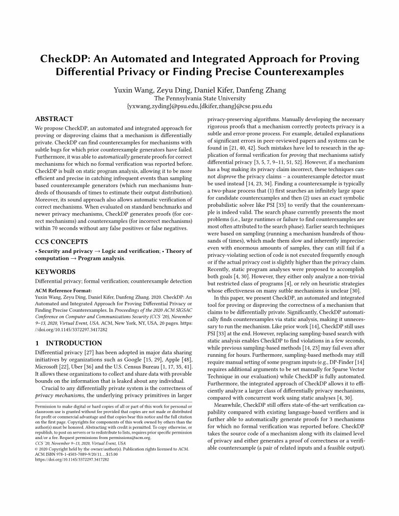
GapSVT. This is an improved (and correct) variant of SVT whichprovides numerical information about some queries. When a noisyquery exceeds the noisy threshold, it outputs the difference betweenthese noisy values; otherwise it returns false. This provides anestimate for how much higher a query is compared to the threshold.The algorithm was first proposed and verified in [51]; its pseudocode is shown in Figure 1. Here, Lap (2/𝜖) draws one sample fromLaplace distribution with mean 0 and scale factor of 2/𝜖 . This ran-dom value is then added to the public threshold 𝑇 (stored as noisythreshold𝑇[ ). For each query answer, another independent Laplacenoise [2 = Lap (4𝑁 /𝜖) is added. If the noisy query answer q[i] +[2 is above the noisy threshold 𝑇[ , the gap between them (q[i] +[2 −𝑇[ ) is added to the output list out, otherwise 0 is added.

One key observation from the manual proofs of SVT and itsvariants [21, 24, 28, 40] is that the privacy cost is only paid forthe queries whose noisy answers are above the noisy threshold. Inother words, outputting false does not incur any new privacy cost.Correspondingly, the correct alignment for GapSVT [24, 51] (that is,the distance that [1 and [2 need to be moved to ensure the outputis the same when the input changes from 𝑞 [𝑖] to 𝑞′[𝑖] ≡ 𝑞 [𝑖] + �� [𝑖],for all 𝑖) is: [1 : 1 and [2 : q[i] + [2 ≥ 𝑇[ ? (1 - q[i]) : 0.

Note that [2 is aligned with non-zero distance only under thetrue branch; hence, no privacy cost is paid in the other branch. Itis easy to verify that if every query has sensitivity 1, the cost of thisalignment is bounded by 𝜖 .

BadGapSVT. We also consider a variant of SVT (and GapSVT)that incorrectly tries to release numerical information. When anoisy query answer is larger than the noisy threshold, the variantreleases that noisy query answer (that is, it does not subtract from itthe noisy threshold); otherwise it outputs false. This is an incorrectvariant of SVT [45] that was reported in [40] and was called iSVT4in [23]. More precisely, BadGapSVT replaces line 7 of GapSVTwith out := (q[i] + [2)::out;. This small change makes itnot 𝜖-differentially private [40]. The reason why is subtle, but theintuition is the following. Suppose BadGapSVT returns a noisyquery answer q[i] + [2 = 3, the attacker is able to deduce that𝑇[ ≤ 3. Once this information is leaked, outputting false in theelse branch is no longer “free”; every output incurs a privacy cost.

2.5 Approach OverviewWe use GapSVT and BadGapSVT to illustrate how CheckDP gener-ates proofs and counterexamples.

Code Transformation (Section 3). CheckDP first takes the proba-bilistic algorithm being checked, written in the CheckDP language

function GapSVT (T,N,size : num0 ,q : list num∗ )

returns (out : list num0 ), check(𝜖)precondition ∀ i. −1 ≤ q[i] ≤ 11 [1 := Lap (2/𝜖)2 𝑇[ := 𝑇 + [1;3 count := 0; i := 0;4 while (count < N ∧ i < size)5 [2 := Lap (4𝑁 /𝜖)6 if (q[i] + [2 ≥ 𝑇[ ) then7 out := (q[i] + [2 - 𝑇[ )::out;8 count := count + 1;9 else

10 out := false::out;11 i := i + 1;

function Transformed GapSVT (T,N,size,q, q, 𝑠𝑎𝑚𝑝𝑙𝑒 , \ )returns (out)12 v𝜖 := 0; idx = 0;

13 [1 := 𝑠𝑎𝑚𝑝𝑙𝑒[idx]; idx := idx + 1;

14 v𝜖 := v𝜖 + |A1 | × 𝜖/2; [1 := A1;

15 𝑇[ := 𝑇 + [1;

16 𝑇[ := [1;

17 count := 0; i := 0;18 while (count < N ∧ i < size)19 [2 := 𝑠𝑎𝑚𝑝𝑙𝑒[idx]; idx := idx + 1;

20 v𝜖 := v𝜖 + |A2 | × 𝜖/4𝑁; [2 := A2;

21 if (q[i] + [2 ≥ 𝑇[ ) then

22 assert(q[i] + [2 + q[i] + [2 ≥ 𝑇[ + 𝑇[);

23 assert(q[i] + [2 - 𝑇[ == 0);

24 out := (q[i] + [2 - 𝑇[ )::out;25 count := count + 1;26 else

27 assert(¬(q[i] + [2 + q[i] + [2 ≥ 𝑇[ + 𝑇[));

28 out := false::out;29 i := i + 1;30 assert(v𝜖 ≤ 𝜖);

Figure 1: GapSVT and its transformed code, where under-lined parts are added by CheckDP. The transformed codecontains two alignment templates for [1 and [2: A1 = \ [0]and A2 = (𝑞 [𝑖] + [2 ≥ 𝑇[ ) ? (\ [1] + \ [2] × 𝑇[ + \ [3] × �� [𝑖]) :(\ [4] +\ [5] ×𝑇[ +\ [6] × �� [𝑖]). The random variables and \ areinserted as part of the function input.

(Section 3.1), and generates the non-probabilistic target code withassertions and alignment templates (i.e. templates for possible align-ments). The bottom of Figure 1 shows the transformed code ofGapSVT with alignment templates. The transformed code is dis-tinguished from the source code in a few important ways: (1) Theprobabilistic sampling commands (at lines 1 and 5) are replacedby non-probabilistic counterparts that read samples from the in-strumented function input 𝑠𝑎𝑚𝑝𝑙𝑒 . (2) An alignment template (e.g.,A1, A2) is generated for each sampling command; each templatecontains a few holes, i.e., \ , which is also instrumented as func-tion input. (3) A distinguished variable v𝜖 is added to track theoverall privacy cost and lines 14 and 20 update the cost variable ina sound way. (4) Assertions are inserted in the transformed code

(lines 22,23,27,30) to ensure the following soundness property:if𝑀 (𝑖𝑛𝑝) is transformed to𝑀 ′(𝑖𝑛𝑝, 𝑖𝑛𝑝, 𝑠𝑎𝑚𝑝𝑙𝑒, \ ), then

∃\ . ∀𝑖𝑛𝑝, 𝑖𝑛𝑝, 𝑠𝑎𝑚𝑝𝑙𝑒. all assertions in𝑀 ′ pass

=⇒ 𝑀 is differentially private

We note that the transformed code forms the basis for both proofand counterexample generation in CheckDP.

Proof/Counterexample Generation (Section 4). Inspired by theCounterexample Guided Inductive Synthesis (CEGIS) [46] tech-nique, originally proposed for program synthesis, CheckDP uses averify-invalidate loop to simultaneously generate proofs and coun-terexamples. Unlike CEGIS, however, the verify-invalidate loopis bidirectional, in the sense that it internally records all previouscounterexamples (resp. proofs) to generate one proof (resp. coun-terexample) as the algorithm output. On the other hand, the CEGISloop is unidirectional: it only collects and uses a set of inputs toguide synthesis internally. At a high level, the verify-invalidateloop of CheckDP includes two integrated sub-loops, one for proofgeneration and the other for counterexample generation.

Verify Sub-loop. Its goal is to generate a proof (i.e., an instantia-tion of \ ) such that ∀𝑖𝑛𝑝, 𝑖𝑛𝑝, 𝑠𝑎𝑚𝑝𝑙𝑒. all assertions in𝑀 ′ pass

This is done by two iterative phases:(1) Generating invalidating inputs: Given a proof candidate (i.e.,

an instantiation of \ ), it is incorrect if∃𝑖𝑛𝑝, 𝑖𝑛𝑝, 𝑠𝑎𝑚𝑝𝑙𝑒. some assertion in𝑀 ′ fails

We use 𝐼 to denote a triple of 𝑖𝑛𝑝, 𝑖𝑛𝑝, 𝑠𝑎𝑚𝑝𝑙𝑒 . Hence, given anyinstantiation of \ , we use an off-the-shelf symbolic executiontool such as KLEE [18] to find invalidating inputs when possible.

(2) Generating proof candidates: with a set of invalidating inputsfound so far 𝐼1, · · · , 𝐼𝑖 , we can try to generate a new proofcandidate to satisfy ∃\ . 𝑀 ′(𝐼1, \ ) ∧ · · · ∧𝑀 ′(𝐼𝑖 , \ ).Starting from a default instantiation (e.g., one that sets ∀𝑖 . \ [𝑖] =

0), CheckDP iteratively repeats Phases 1 and 2. Since CheckDP usesall invalidating inputs found so far in Phase 2, the proof candidateafter each iteration is improving.When Phase 1 gets stuck, CheckDPobtains a proof candidate \ which is a privacy proof if

∀𝑖𝑛𝑝, 𝑖𝑛𝑝, 𝑠𝑎𝑚𝑝𝑙𝑒. 𝑀 ′(𝑖𝑛𝑝, 𝑖𝑛𝑝, 𝑠𝑎𝑚𝑝𝑙𝑒, \ )due to the soundness property above. Hence, a proof (alignment) canbe validated by program verification tools such as CPAChecker [13].For GapSVT, CheckDP generates and verifies (via CPAChecker) that\ = {1, 1, 0,−1, 0, 0, 0} results in a proof that GapSVT satisfies 𝜖-differential privacy.

Invalidate Sub-loop. While the verify sub-loop is conceptuallysimilar to a CEGIS loop [46], CheckDP also employs an invalidatesub-loop (integrated with the verify sub-loop); its goal is to generateone invalidating input 𝐼 such that ∀\ . some assertion in𝑀 ′ fail. Thisis done by two iterative phases:2

(1) Generating proof candidates: Given an invalidating input 𝐼 ,it is incorrect if ∃\ . 𝑀 ′(𝐼 , \ ). Hence, given any 𝐼 , we can useKLEE [18] to find an alignment when possible.

2Note that a set of invalidating inputs 𝐼1, · · · , 𝐼𝑖 , generated from Phase 2 of the verifysub-loop is not a counterexample candidate, since by definition, a differential privacycounterexample consists of only one invalidating input.

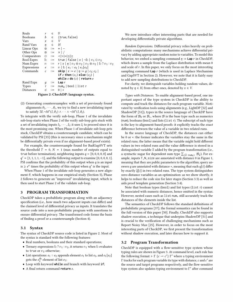
Reals 𝑟 ∈ RBooleans 𝑏 ∈ {true, false}Vars 𝑥 ∈ VRand Vars [ ∈ HLinear Ops ⊕ ::= + | −Other Ops ⊗ ::= × | /Comparators ⊙ ::= < |> |=|≤|≥Bool Exprs b ::= true | false | 𝑥 | ¬b | n1 ⊙ n2Num Exprs n ::= 𝑟 | 𝑥 | [ | n1 ⊕ n2 | n1 ⊗ n2 | b ? n1 : n2Expressions 𝑒 ::= n | b | 𝑒1 :: 𝑒2 | 𝑒1 [𝑒2]Commands 𝑐 ::= skip | 𝑥 := 𝑒 | [ := 𝑔 | 𝑐1; 𝑐2 |

if 𝑒 then (𝑐1) else (𝑐2) |while 𝑒 do (𝑐) | return 𝑒

Rand Exps 𝑔 ::= Lap 𝑟Types 𝜏 ::= numd | bool | list 𝜏Distances d ::= 0 | ∗

Figure 2: CheckDP: language syntax.

(2) Generating counterexamples: with a set of previously foundalignments \1, · · · , \𝑖 , we try to find a new invalidating inputto satisfy ∃𝐼 .¬𝑀 ′(𝐼 , \1) ∧ · · · ∧ ¬𝑀 ′(𝐼 , \𝑖 ).

To integrate with the verify sub-loop, Phase 1 of the invalidatesub-loop starts when Phase 2 of the verify sub-loop gets stuck witha set of invalidating inputs 𝐼1, · · · , 𝐼𝑖 ; it uses 𝐼𝑖 to proceed since it isthe most promising one. When Phase 1 of invalidate sub-loop getsstuck, CheckDP obtains a counterexample candidate, which can bevalidated by PSI [33] (this is necessary since a mechanism mightbe differentially private even if no alignment-based proof exists).

For example, the counterexample found for BadGapSVT setsthe threshold 𝑇 = 0, 𝑁 = 1 (max number of outputs equal totrue before termination), neighboring inputs 𝑞 = [0, 0, 0, 0, 0] and𝑞′ = [1, 1, 1, 1,−1], and the following output to examine [0, 0, 0, 0, 1].PSI confirms that the probability of this output when 𝑞 is an inputis ≥ 𝑒𝜖 times the probability of this output when 𝑞′ is the input.

When Phase 1 of the invalidate sub-loop generates a new align-ment \ , which happens in our empirical study (Section 5), Phase2 follows to generate an “improved” invalidating input, which isthen used to start Phase 2 of the validate sub-loop.

3 PROGRAM TRANSFORMATIONCheckDP takes a probablistic program along with an adjacencyspecification (i.e., how much two adjacent inputs can differ) andthe claimed level of differential privacy as inputs. It translates thesource code into a non-probabilistic program with assertions toensure differential privacy. The transformed code forms the basisof finding a proof or a counterexample (Section 4).

3.1 SyntaxThe syntax of CheckDP source code is listed in Figure 2. Most ofthe syntax is standard with the following features:• Real numbers, booleans and their standard operations;• Ternary expressions b ? n1 : n2, it returns n1 when b evaluatesto true or n2 otherwise;• List operations: 𝑒1 :: 𝑒2 appends element 𝑒1 to list 𝑒2, and 𝑒1 [𝑒2]gets the 𝑒th2 element of list 𝑒1;• Loop with keyword while and branch with keyword if;• A final return command return 𝑒 .

We now introduce other interesting parts that are needed fordeveloping differentially private algorithms.

Random Expressions. Differential privacy relies heavily on prob-abilistic computations: many mechanisms achieve differential pri-vacy by adding appropriate random noise to variables. Tomodel thisbehavior, we embed a sampling command [ := Lap 𝑟 in CheckDP,which draws a sample from the Laplace distribution with mean 0and scale of 𝑟 . In this paper, we only focus on the most interestingsampling command Lap 𝑟 (which is used in Laplace Mechanismand GapSVT in Section 2). However, we note that it is fairly easyto add new sampling distributions to CheckDP.

For clarity, we distinguish variables holding random values, de-noted by [ ∈ H, from other ones, denoted by 𝑥 ∈ V.

Types with Distances. To enable alignment-based proof, one im-portant aspect of the type system in CheckDP is the ability tocompute and track the distances for each program variable. Moti-vated by verification tools using alignments (e.g., LightDP [52] andShadowDP [51]), types in the source language of CheckDP havethe form of B0 or B∗, where B is the base type such as numerics(num), booleans (bool) and lists (list 𝜏 ). The subscript of each typeis the key to alignment-based proofs: it explicitly tracks the exactdifference between the value of a variable in two related runs.

In the source language of CheckDP, the distances can eitherbe 0 or ∗: the former indicates the variables stay the same in therelated runs; the latter means that the variable might hold differentvalues in two related runs and the value difference is stored in adistinguished variable �� added by the program transformation (i.e.,a syntactic sugar for dependent sum type

∑(�� : num0) B�� ). For ex-

ample, inputs T,N,size are annotated with distance 0 in Figure 1,meaning that they are public parameters to the algorithm; query an-swers 𝑞 are annotated with distance ∗, meaning that each 𝑞 [𝑖] differby exactly �� [𝑖] in two related runs. The type system distinguisheszero-distance variables as an optimization: as we show shortly, ithelps to reduce the code size for later stages (Section 3.3) as well asaids proof template generation (Section 3.4).

Note that boolean types (bool) and list types (list 𝜏) cannotbe associated with numeric distances, hence omitted in the syntax.However, nested cases such as list num∗ still accurately track thedistances of the elements inside the list.

The semantics of CheckDP follows the standard definitions ofprobabilistic programs [37]; the formal semantics can be found inthe full version of this paper [50]. Finally, CheckDP also supportsshadow execution, a technique that underpins ShadowDP [51] andis crucial to the verification of challenging mechanisms such asReport Noisy Max [25]. However, in order to focus on the mostinteresting parts of CheckDP, we first present the transformationwithout shadow execution, and later discuss how to support it.

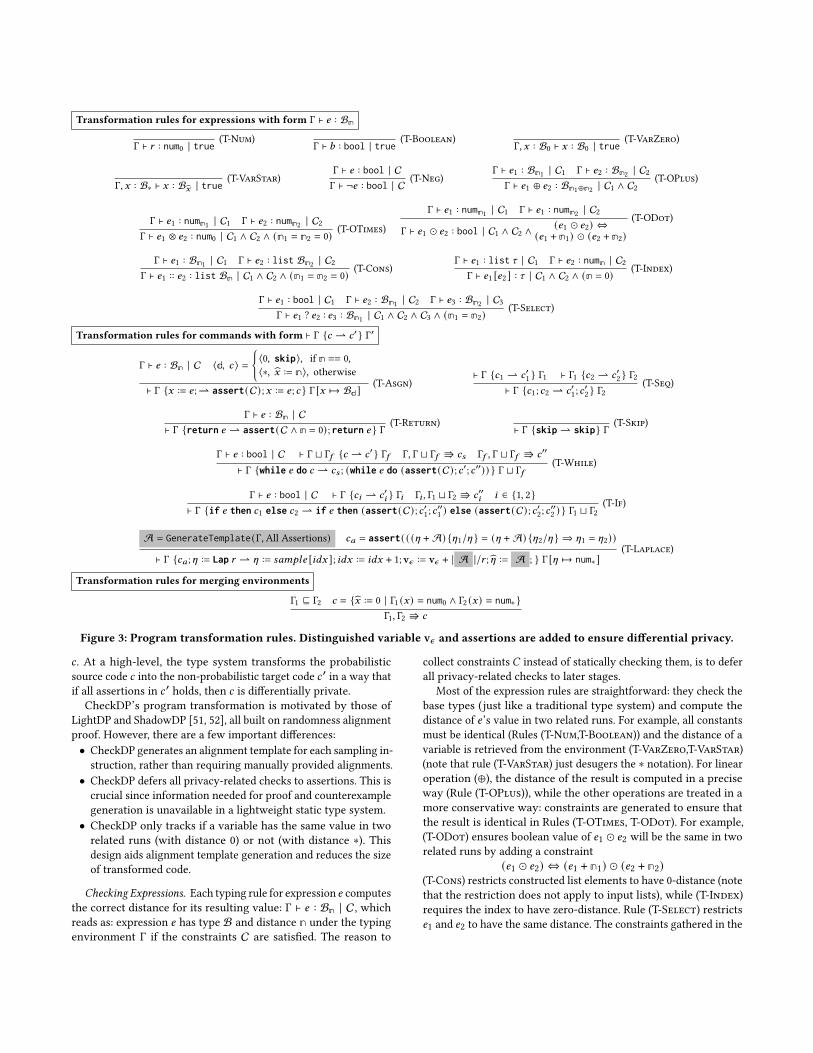
3.2 Program TransformationCheckDP is equipped with a flow-sensitive type system whosetyping rules are shown in Figure 3. At command level, each rule hasthe following format: ⊢ Γ {𝑐 ⇀ 𝑐 ′} Γ′ where a typing environmentΓ tracks for each program variable its typewith distance, 𝑐 and 𝑐 ′ arethe source and target programs respectively, and the flow-sensitivetype system also updates typing environment to Γ′ after command

Transformation rules for expressions with form Γ ⊢ 𝑒 : Bn

Γ ⊢ 𝑟 : num0 | true(T-Num)

Γ ⊢ 𝑏 : bool | true (T-Boolean)Γ, 𝑥 : B0 ⊢ 𝑥 : B0 | true

(T-VarZero)

Γ, 𝑥 : B∗ ⊢ 𝑥 : B𝑥 | true(T-VarStar)

Γ ⊢ 𝑒 : bool | CΓ ⊢ ¬𝑒 : bool | C (T-Neg)

Γ ⊢ 𝑒1 : Bn1 | C1 Γ ⊢ 𝑒2 : Bn2 | C2Γ ⊢ 𝑒1 ⊕ 𝑒2 : Bn1⊕n2 | C1 ∧ C2

(T-OPlus)

Γ ⊢ 𝑒1 : numn1 | C1 Γ ⊢ 𝑒2 : numn2 | C2Γ ⊢ 𝑒1 ⊗ 𝑒2 : num0 | C1 ∧ C2 ∧ (n1 = n2 = 0) (T-OTimes)

Γ ⊢ 𝑒1 : numn1 | C1 Γ ⊢ 𝑒1 : numn2 | C2

Γ ⊢ 𝑒1 ⊙ 𝑒2 : bool | C1 ∧ C2 ∧(𝑒1 ⊙ 𝑒2) ⇔

(𝑒1 + n1) ⊙ (𝑒2 + n2)(T-ODot)

Γ ⊢ 𝑒1 : Bn1 | C1 Γ ⊢ 𝑒2 : list Bn2 | C2Γ ⊢ 𝑒1 :: 𝑒2 : list Bn | C1 ∧ C2 ∧ (n1 = n2 = 0) (T-Cons)

Γ ⊢ 𝑒1 : list 𝜏 | C1 Γ ⊢ 𝑒2 : numn | C2Γ ⊢ 𝑒1 [𝑒2 ] : 𝜏 | C1 ∧ C2 ∧ (n = 0) (T-Index)

Γ ⊢ 𝑒1 : bool | C1 Γ ⊢ 𝑒2 : Bn1 | C2 Γ ⊢ 𝑒3 : Bn2 | C3Γ ⊢ 𝑒1 ? 𝑒2 : 𝑒3 : Bn1 | C1 ∧ C2 ∧ C3 ∧ (n1 = n2)

(T-Select)

Transformation rules for commands with form ⊢ Γ {𝑐 ⇀ 𝑐′ } Γ′

Γ ⊢ 𝑒 : Bn | C ⟨d, 𝑐 ⟩ ={⟨0, skip⟩, if n == 0,⟨∗, �� := n⟩, otherwise

⊢ Γ {𝑥 := 𝑒 ;⇀ assert(C) ;𝑥 := 𝑒 ;𝑐 } Γ [𝑥 ↦→ Bd ](T-Asgn)

⊢ Γ {𝑐1 ⇀ 𝑐′1 } Γ1 ⊢ Γ1 {𝑐2 ⇀ 𝑐′2 } Γ2⊢ Γ {𝑐1;𝑐2 ⇀ 𝑐′1;𝑐

′2 } Γ2

(T-Seq)

Γ ⊢ 𝑒 : Bn | C⊢ Γ {return 𝑒 ⇀ assert(C ∧ n = 0) ; return 𝑒 } Γ (T-Return) ⊢ Γ {skip ⇀ skip} Γ (T-Skip)

Γ ⊢ 𝑒 : bool | C ⊢ Γ ⊔ Γ𝑓 {𝑐 ⇀ 𝑐′ } Γ𝑓 Γ, Γ ⊔ Γ𝑓 ⇛ 𝑐𝑠 Γ𝑓 , Γ ⊔ Γ𝑓 ⇛ 𝑐′′

⊢ Γ {while 𝑒 do 𝑐 ⇀ 𝑐𝑠 ; (while 𝑒 do (assert(C) ;𝑐′;𝑐′′)) } Γ ⊔ Γ𝑓(T-While)

Γ ⊢ 𝑒 : bool | C ⊢ Γ {𝑐𝑖 ⇀ 𝑐′𝑖 } Γ𝑖 Γ𝑖 , Γ1 ⊔ Γ2 ⇛ 𝑐′′𝑖 𝑖 ∈ {1, 2}⊢ Γ {if 𝑒 then 𝑐1 else 𝑐2 ⇀ if 𝑒 then (assert(C) ;𝑐′1;𝑐′′1 ) else (assert(C) ;𝑐′2;𝑐′′2 ) } Γ1 ⊔ Γ2

(T-If)

A = GenerateTemplate(Γ,All Assertions) 𝑐𝑎 = assert( ( ([ + A) {[1/[ } = ([ + A) {[2/[ } ⇒ [1 = [2))

⊢ Γ {𝑐𝑎 ;[ := Lap 𝑟 ⇀ [ := 𝑠𝑎𝑚𝑝𝑙𝑒 [𝑖𝑑𝑥 ]; 𝑖𝑑𝑥 := 𝑖𝑑𝑥 + 1; v𝜖 := v𝜖 + | A |/𝑟 ; [ := A ; } Γ [[ ↦→ num∗ ](T-Laplace)

Transformation rules for merging environments

Γ1 ⊑ Γ2 𝑐 = {�� := 0 | Γ1 (𝑥) = num0 ∧ Γ2 (𝑥) = num∗ }Γ1, Γ2 ⇛ 𝑐

Figure 3: Program transformation rules. Distinguished variable v𝜖 and assertions are added to ensure differential privacy.

𝑐 . At a high-level, the type system transforms the probabilisticsource code 𝑐 into the non-probabilistic target code 𝑐 ′ in a way thatif all assertions in 𝑐 ′ holds, then 𝑐 is differentially private.

CheckDP’s program transformation is motivated by those ofLightDP and ShadowDP [51, 52], all built on randomness alignmentproof. However, there are a few important differences:• CheckDP generates an alignment template for each sampling in-struction, rather than requiring manually provided alignments.• CheckDP defers all privacy-related checks to assertions. This iscrucial since information needed for proof and counterexamplegeneration is unavailable in a lightweight static type system.• CheckDP only tracks if a variable has the same value in tworelated runs (with distance 0) or not (with distance ∗). Thisdesign aids alignment template generation and reduces the sizeof transformed code.

Checking Expressions. Each typing rule for expression 𝑒 computesthe correct distance for its resulting value: Γ ⊢ 𝑒 : Bn | C, whichreads as: expression 𝑒 has type B and distance n under the typingenvironment Γ if the constraints C are satisfied. The reason to

collect constraints 𝐶 instead of statically checking them, is to deferall privacy-related checks to later stages.

Most of the expression rules are straightforward: they check thebase types (just like a traditional type system) and compute thedistance of 𝑒’s value in two related runs. For example, all constantsmust be identical (Rules (T-Num,T-Boolean)) and the distance of avariable is retrieved from the environment (T-VarZero,T-VarStar)(note that rule (T-VarStar) just desugers the ∗ notation). For linearoperation (⊕), the distance of the result is computed in a preciseway (Rule (T-OPlus)), while the other operations are treated in amore conservative way: constraints are generated to ensure thatthe result is identical in Rules (T-OTimes, T-ODot). For example,(T-ODot) ensures boolean value of 𝑒1 ⊙ 𝑒2 will be the same in tworelated runs by adding a constraint

(𝑒1 ⊙ 𝑒2) ⇔ (𝑒1 + n1) ⊙ (𝑒2 + n2)(T-Cons) restricts constructed list elements to have 0-distance (notethat the restriction does not apply to input lists), while (T-Index)requires the index to have zero-distance. Rule (T-Select) restricts𝑒1 and 𝑒2 to have the same distance. The constraints gathered in the

expression rules will later be explicitly instrumented as assertionsin the translated programs, which we will explain shortly.

3.3 Checking CommandsFor each program statement, the type system updates the typing en-vironment and if necessary, instruments code to update �� variablesto the correct distances. Moreover, it ensures that the two relatedruns take the same branch in if-statement and while-statement.

Flow-Sensitivity. Each typing rule updates the typing environ-ment to track if a variable has zero-distance. When a variable hasnon-zero distance, it instruments the source code to properly main-tain the corresponding �� variables. The most interesting rules are:rule (T-Asgn) properly promotes the type of 𝑥 to be B∗ (tracked bydistance variables) in Γ′ if the distance of 𝑒 is not 0. Meanwhile itoptimizes away updates to x and properly downgrades type to B0if 𝑒 has a zero-distance. For example, line 16 in GapSVT (Figure 1)is instrumented to update distance of 𝑇[ , according to the distanceof𝑇 +[1. Moreover, variable count in GapSVT always has the typenum0; therefore its distance variable never appears in the translatedprogram due to the optimization in (T-Asgn).

Rule (T-If) and (T-While) are more complicated since they bothneed to merge environments. In rule (T-If), as 𝑐1 and 𝑐2 mightupdate Γ to Γ1 and Γ2 respectively, we need to merge them in anatural way: the distance of a type form a two-level lattice with0 ⊏ ∗. Thus we define a union operator ⊔ for distances d as:

d1 ⊔ d2 ≜

{d1 if d1 = d2∗ otherwise

therefore the union operator for two environments are defined asfollows: Γ1 ⊔ Γ2 = _𝑥. Γ1 [𝑥] ⊔ Γ2 [𝑥].

Moreover, we use an auxiliary function Γ1, Γ2 ⇛ 𝑐 to “promote”a variable to star type. For example, with Γ(𝑥) = ∗, Γ(𝑦) = ∗ andΓ(𝑏) = 0, rule (T-If) translates the source codeif 𝑏 then 𝑥 := 𝑦 else 𝑥 := 1 to the following:if 𝑏 then (𝑥 := 𝑦; �� := ��; ) else (𝑥 := 1; �� := 0)where �� := �� is instrumented by (T-Asgn) and �� := 0 is instru-mented due to the promotion.

Similarly, the typing environments are merged in rule (T-While),except that it requires a fixed point Γ𝑓 such that ⊢ Γ ⊔ Γ𝑓 {𝑐} Γ𝑓 .We follow the construction in [51] to compute a fixed point, notingthat the computation always terminates since all of the translationrules are monotonic and the lattice only has two levels.

Assertion Generation. To ensure differential privacy, the typesystem inserts assertion in various rules:• To ensure that two related runs take the same control flow,(T-If) and (T-While) asserts constraints gathered from makingsure that the boolean has zero-distance (e.g., from (T-ODot)).As an optimization, we use the branch condition to simplifyconstraints when possible. For example, constraints 𝑒1 ⊙ 𝑒2 ⇔(𝑒1 +n1) ⊙ (𝑒2 +n2) are simplified as (𝑒1 +n1) ⊙ (𝑒2 +n2) (resp.¬((𝑒1 + n1) ⊙ (𝑒2 + n2))) in the true (resp. false) branch.• To ensure that the final output value is differentially private,rule (T-Return) asserts that its distance is zero (i.e., identicalin two related runs).

• To ensure all constraints collected in the expression rules aresatisfied, assignment rules (T-Asgn) and (T-AsgnStar) alsoinsert corresponding assertions.

3.4 Checking Sampling CommandsRule (T-Laplace) performs a few important tasks:

Replacing Sampling Command. Rule (T-Laplace) removes thesampling instruction and assign to [ the next (unknown) samplevalue sample[idx], where sample is a parameter of type list numadded to the transformed code. The typing rule also increments idxso that the next sampling command will read out the next value.

Checking Injectivity. T-Laplace adds an assertion 𝑐𝑎 to check theinjectivity of the generated alignment (a fundamental requirementof alignment-based proofs): the same aligned value of [ implies thesame value of [ in the original execution.

Tracking Privacy Cost. A distinguished privacy cost variable v𝜖is also instrumented to track the cost for aligning the random vari-ables in the program. Due to the properties of Laplace distribution,for a sampling command [ := Lap 𝑟 with alignment template A,we have P([)/P([ + A) ≤ 𝑒|A |/𝑟 . Hence, the privacy cost foraligning [ by A is |A| /𝑟 . Note that the symbols in gray, includ-ing A, are placeholders when the rule is applied, since functionGenerateTemplate takes all assertions in the transformed code asinputs. Once translation is complete, the placeholders are filled inby the algorithm that we discuss in Section 4.

Alignment Template Generation. For each sampling command[ := Lap 𝑟 , an alignment of [ is needed in a randomness alignmentproof. In its most flexible form, the alignment can be written asany numerical expression n, which is prohibitive for our goal ofautomatic proof generation. On the other hand, using simple heuris-tics such as only considering constant alignment does not work:for example, the correct alignment for [2 in GapSVT is written as“(q[i] + [2 ≥ 𝑇[ ) ? (1 − q[i]) : 0”, where the alignment actuallydepends on which branch is taken during the execution.

To tackle the challenges, CheckDP generates an alignment tem-plate for each sampling instruction; a template is a numerical ex-pression with “holes” whose values are to be searched for in laterstages. For example, the template generated for [2 in GapSVT is

(q[i] + [2 ≥ 𝑇[ )?(\ [0] + \ [1] ×𝑇[ + \ [2] × q[i]):

(\ [3] + \ [4] ×𝑇[ + \ [5] × q[i])where \ [0] − \ [5] are symbolic coefficients to be found later.

In general, for each sampling command [ = Lap 𝑟 , CheckDPfirst uses static program analysis to find a set of relevant programexpressions, denoted by E, and a set of relevant program variables,denoted by V (as described shortly). Second, it generates an align-ment template as follows:

AE ::=

{𝑒0 ? AE\{𝑒0 } :AE\{𝑒0 } , when E = {𝑒0, · · · }\0 +

∑𝑣𝑖 ∈V \𝑖 × 𝑣𝑖with fresh \0, · · · , \ |V | , otherwise

where \ denotes coefficients (“holes”) to be filled out out by laterstages and each of them is generated fresh.

To find proper E and V, our insight is that the alignments serveto “cancel out” the differences between two related runs (i.e., to

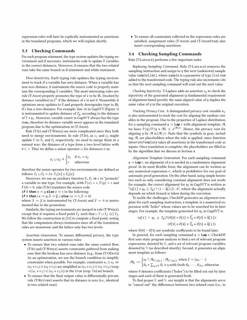
make all assertions pass). Algorithm 1 follows the insight to com-pute E and V for each sampling instruction: it takes Γ𝑠 , the typingenvironment right before the sampling instruction and 𝐴, all asser-tions in the transformed code, as inputs. It also assumes an oracleDepends(𝑒, 𝑥) which returns true whenever the expression 𝑒 de-pends on the variable 𝑥 . We note that the oracle can be implementedas standard program dependency analysis [2, 31] or informationflow analysis [12]; hence, we omit the details in this paper.

Algorithm 1: Template generation for [ := Lap 𝑟

input :Γ𝑠 : typing environment at sampling command𝐴: set of the generated assertions in the program

1 function GenerateTemplate(Γ𝑠 , 𝐴):2 E← ∅, V← ∅3 foreach assert(𝑒) ∈ 𝐴 do4 if Depends(𝑒, [) then5 if assert(𝑒) is generated by (T-If) then6 𝑒 ′ ← the branch condition of if7 E← E ∪ {𝑒 ′}8 foreach 𝑣 ∈ 𝑉𝑎𝑟𝑠 ∪ {𝑒1 [𝑒2] |𝑒1 [𝑒2] ∈ 𝑒} do9 if Γ𝑠 ⊢ 𝑣 : B0 ∧ Depends(𝑒, 𝑣) then10 V← V ∪ {𝑣}

11 foreach 𝑒 ∈ E ∪ V do12 remove 𝑒 from E and V if not in scope13 return E,V;

The algorithm first checks (at line 4) if aligning [ has a chance tomake an assertion pass. If so, it will increment E and V as follows.For E, we notice that only for the assertions generated by rule (T-If),depending on the branch condition allows the alignment to havedifferent values under different branches. Hence, we add the branchcondition to E in this case. For V, our goal is to use the alignment to“cancel” the differences caused by other variables and array elementssuch as 𝑞 [𝑖] used in 𝑒 . Hence, we only need to consider �� if (1) 𝑣is different between two related runs (i.e., Γ𝑠 ⊢ 𝑣 : B0) and (2) 𝑣contributes the assertion (i.e., 𝑒 depends on 𝑣).

Finally, the algorithm performs a “scope check”: if any element inE orV contains out-of-scope variables, then the element is excluded;for example, [1 should not depend on 𝑞 [𝑖] in GapSVT since 𝑞 [𝑖],essentially an iterator of 𝑞, is not in scope at that point.

Consider [1 and [2 in GapSVT. The assertions in the translatedprograms are (we only list the assertion in the true branch sincethe constraint in false branch is symmetric) :(1) assert(q[i] + [2 + q[i] + [2 ≥ 𝑇[ + 𝑇[)

(2) assert(q[i] + [2 - 𝑇[ = 0)

For [1, we have Γ𝑠 = {q : ∗} (we omit the base types and the vari-ables that have 0 distance for brevity) and both assertions dependon [1. Since both assertions depend on [1 and q[i], Algorithm 1adds q[i] into V. Moreover, assertion (1) is generated by rule (T-If).Thus,the algorithm adds q[i] + [2 ≥ 𝑇[ into E. Finally, sinceq[i] is out of scope at the sampling instruction, expression usingq[i] and variable q[i] are excluded, resulting V ={ } and E ={ }.

For [2, we have Γ𝑠 = {q: *,𝑇[ : *}. Since both assertions depend on[2 and q[i] and 𝑇 , Algorithm 1 adds q[i] and 𝑇[ into V. Similarto [1, the algorithm also adds q[i] + [2 ≥ 𝑇[ into E. Finally, all

expressions and variable are in scope, resulting V ={q[i], 𝑇[ } andE ={q[i] + [2 ≥ 𝑇[ }.

3.5 Function Signature RewriteFinally, CheckDP rewrites the function signature to reflect theextra parameters and holes introduced in the transformed code.In general, 𝑀 (𝑖𝑛𝑝) is transformed to a new function signature𝑀 ′(𝑖𝑛𝑝, 𝑖𝑛𝑝, 𝑠𝑎𝑚𝑝𝑙𝑒, \ ) where 𝑖𝑛𝑝 are the distance variables asso-ciated with inputs whose distance is not zero (e.g., �� is associatedwith 𝑞 in GapSVT), 𝑠𝑎𝑚𝑝𝑙𝑒 is a list of random values used in 𝑀 ,and \ are the missing holes in alignment templates.

3.6 Shadow ExecutionTo tackle challenging mechanisms such as Report Noisy Max [25],CheckDP uses shadow execution [51]. Intuitively, the shadow exe-cution tracks another program execution where the injected noisesare always the same as those in the original execution. Therefore,values computed in the shadow execution incur no privacy cost.The aligned execution can then switch to shadow execution whencertain conditions are met, allowing extra permissiveness [51].

Supporting shadow execution only requires a few modifications:(1) Expressions will have a pair of distances (⟨d◦, d†⟩), where the

extra distance d† tracks the distance in the shadow execution;(2) Since the branches and loop conditions in shadow execution

are not aligned, they might diverge from the original execution.Hence, a separate shadow branch/loop is generated to correctlyupdate the shadow distances for the variables.Since the extended transformation rules largely follow the cor-

responding typing rules of ShadowDP, we present the complete setof rules with detailed explanations in the Appendix.

3.7 SoundnessCheckDP enforces a fundamental property: suppose𝑀 (𝑖𝑛𝑝) is trans-formed to𝑀 ′(𝑖𝑛𝑝, 𝑖𝑛𝑝, 𝑠𝑎𝑚𝑝𝑙𝑒, \ ), then𝑀 (𝑖𝑛𝑝) is differentially pri-vate if there is a list of values of \ , such that all assertions in 𝑀 ′

hold for all 𝑖𝑛𝑝, 𝑖𝑛𝑝, 𝑠𝑎𝑚𝑝𝑙𝑒 . Recall that an alignment template Ais a function of \ . Hence, we have a concrete alignment A(\ ) (i.e.,a proof) when such values of \ exist.

We build the soundness of CheckDP based on that of Shad-owDP [51]. The main difference is that ShadowDP requires everysampling command [ := Lap 𝑟 to be manually annotated. Thus,we can easily rewrite a program𝑀 in CheckDP to a program �� inShadowDP by adding the following annotations:[ := Lap 𝑟 → [ := Lap 𝑟 ; ◦; A[ (\ ) (CheckDP to ShadowDP)where A[ is the alignment template for [. We formalize the mainsoundness results next; the full proof can be found in the full versionof this paper [50].

Theorem 2 (Soundness). Let 𝑀 be a mechanism written inCheckDP. With a list of concrete values of \ , let �� be the correspond-ing mechanism in ShadowDP by rule (CheckDP to ShadowDP). If(1) 𝑀 type checks, i.e., ⊢ Γ {𝑀 ⇀ 𝑀 ′} Γ′ and (2) the assertions in𝑀 ′ hold for all inputs. Then �� type checks in ShadowDP, and theassertions in �� ′ (transformed from �� by ShadowDP) pass.

Theorem 3 (Privacy). With exactly the same notation and as-sumption as Theorem 2,𝑀 satisfies 𝜖-differential privacy.

Invalidating InputGeneration

Proof Generation𝐼!,⋯ , 𝐼"

𝜃"

Counterexample Generation

Verifier

𝜃"

CheckDP

Restart

PSI

𝜃!,⋯ ,𝜃"

𝐼!"#

Verify Sub-loop Exit

Unknown

Proof

𝐶

𝜃! 𝐼"

𝜃"

𝐼"

Counterexample

Invalidate Sub-loop

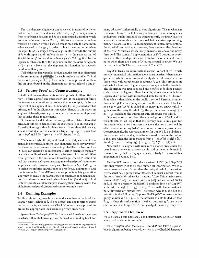
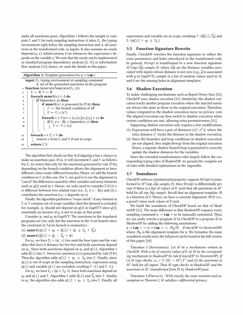
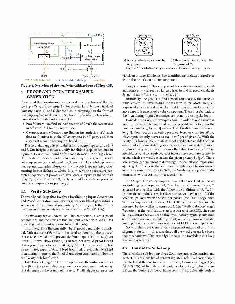
Figure 4: Overviewof the verify-invalidate loop ofCheckDP.

4 PROOF AND COUNTEREXAMPLEGENERATION

Recall that the transformed source code has the form of the fol-lowing:𝑀 ′(𝑖𝑛𝑝, 𝑖𝑛𝑝, 𝑠𝑎𝑚𝑝𝑙𝑒, \ ). For brevity, Let 𝐼 denote a triple of(𝑖𝑛𝑝, 𝑖𝑛𝑝, 𝑠𝑎𝑚𝑝𝑙𝑒), and 𝐶 denote a counterexample in the form of𝐶 = (𝑖𝑛𝑝, 𝑖𝑛𝑝 ′, 𝑜) as defined in Section 2.3. Proof/counterexamplegeneration is divided into two tasks:• Proof Generation: find an instantiation of \ such that assertionsin𝑀 ′ never fail for any input 𝐼 , or• Counterexample Generation: find an instantiation of 𝐼 , suchthat no \ exists to make all assertions in 𝑀 ′ pass, and thenconstruct a counterexample 𝐶 based on 𝐼 .The key challenge here is the infinite search space of both \

and 𝐼 . Our insight is to use a verify-invalidate loop, as depicted inFigure 4, to improve \ and 𝐼 after each iteration. At a high-level,the iterative process involves two sub-loops: the (green) verifysub-loop generates proofs, and the (blue) invalidate sub-loop gener-ates counterexamples. Moreover, the two sub-loops are integrated:starting from a default \0 where \0 [𝑖] = 0. ∀𝑖 , the procedure gen-erates sequences of proofs and invalidating inputs in the form of\0, 𝐼0, \1, 𝐼1, · · · . The final \𝑘 or 𝐼𝑘 is used to construct proof orcounterexamples correspondingly.

4.1 Verify Sub-LoopThe verify sub-loop that involves Invalidating Input Generationand Proof Generation components is responsible of generating asequence of improving alignments \0, \1, · · · , \𝑖 such that, if themechanism is correct, \𝑖 is a privacy proof (i.e, ∀𝐼 . 𝑀 ′(𝐼 , \𝑖 )).

Invalidating Input Generation. This component takes a proofcandidate \𝑖 and then tries to find an input 𝐼𝑖 such that ¬𝑀 ′(𝐼𝑖 , \𝑖 )(meaning that at least one assertion in𝑀 ′ fails).

Intuitively, \𝑖 is the currently “best” proof candidate (initially,a default null proof \0 = [0, · · · ] is used to bootstrap the process)that is able to validate all previously found inputs (𝐼0, · · · , 𝐼𝑖−1). Aninput 𝐼𝑖 , if any, shows that \𝑖 is in fact not a valid proof (recallthat a proof needs to ensure 𝑀 ′(𝐼 , \𝑖 ) ∀𝐼 ). Hence, we call such 𝐼𝑖an invaliding input of \𝑖 and feed it with all previously identifiedinvalidating inputs to the Proof Generation component followingthe “Verify Sub-loop” edge.

Take GapSVT (Figure 1) for example. Since the initial null proof\0 = [0, · · · ] does not align any random variable, any input, say 𝐼0,that diverges on the branch 𝑞 [𝑖] + [2 ≥ 𝑇 will trigger an assertion

Input Space

𝐼0 𝜃1𝐼$𝜃2

(a) A case where \𝑖 cannot beimproved.

Input Space

𝐼0𝜃1

𝐼$ …

𝜃2

(b) Iteratively improving thealignment \𝑖 .

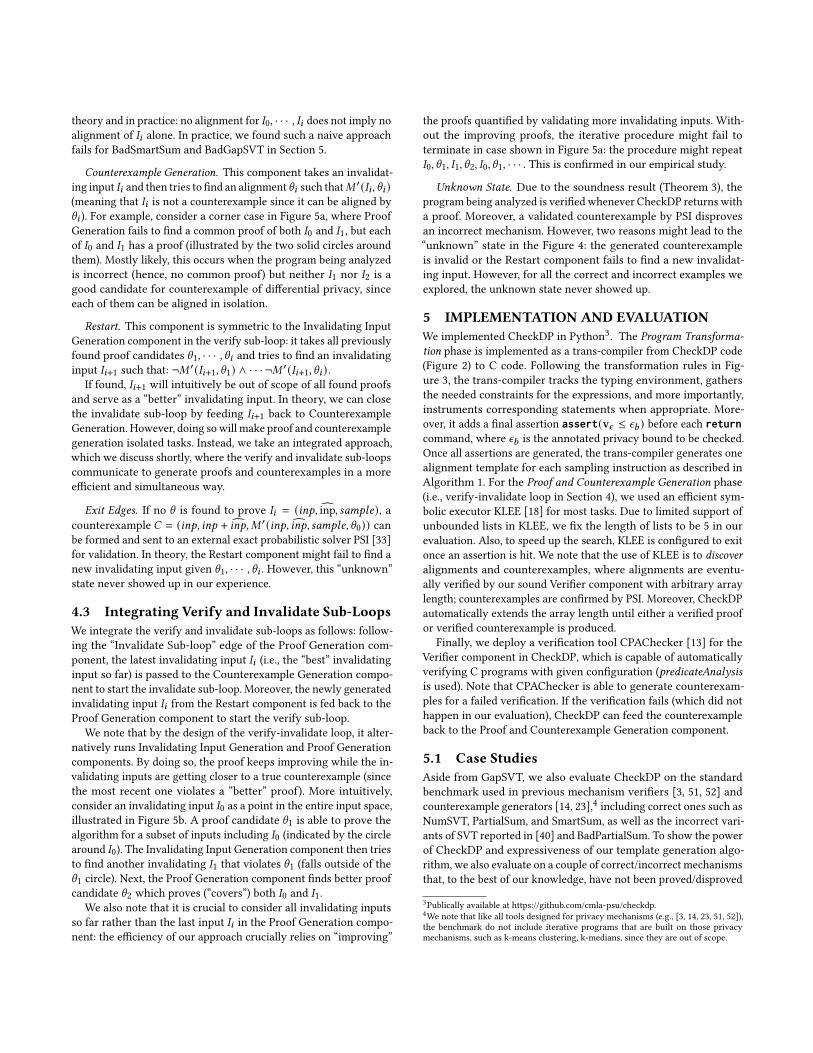
Figure 5: Tentative alignments and invalidating inputs.

violation at Line 22. Hence, the identified invalidating input 𝐼0 isfed to the Proof Generation component.

Proof Generation. This component takes in a series of invalidat-ing inputs 𝐼0, · · · , 𝐼𝑖 seen so far, and tries to find an proof candidate\𝑖 such that:𝑀 ′(𝐼0, \𝑖 ) ∧ · · · ∧𝑀 ′(𝐼𝑖 , \𝑖 ).

Intuitively, the goal is to find a proof candidate \𝑖 that success-fully “covers” all invalidating inputs seen so far. Most likely, animproved proof candidate \𝑖 that is able to align randomness formore inputs is generated by the component. Then \𝑖 is fed back tothe Invalidating Input Generation component, closing the loop.

Consider the GapSVT example again. In order to align random-ness for the invalidating input 𝐼0, one possible \1 is to align therandom variable [2 by −�� [𝑖] to cancel out the difference introducedby 𝑞 [𝑖]. Note that this tentative proof \1 does not work for all pos-sible inputs: it only serves as the “best” proof given 𝐼0. With theVerify Sub-loop, such imperfect proof candidates enable the gen-eration of more invalidating inputs, such as an invalidating input𝐼1 where the query answers are mostly below the threshold 𝑇 (𝐼1invalidates \1 since a privacy cost incurs whenever any branch istaken, which eventually exhausts the given privacy budget). There-fore, a more general proof that leverages the conditional expression𝑞 [𝑖] + [2 ≥ 𝑇 ? • : • in the alignment template can be discoveredby Proof Generation. For GapSVT, the Verify sub-loop eventuallyterminates with a correct proof (Section 5).

Exit Edges. The verify loop has two exit edges. First, when noinvalidating input is generated, \𝑖 is likely a valid proof. Hence, \𝑖is passed to a verifier with the following condition: ∀𝐼 . 𝑀 ′(𝐼 , \𝑖 ) .Due to the soundness result (Theorem 3), we have a proof of dif-ferential privacy when the verifier passes (the “Exit” edge fromVerifier component). Otherwise, CheckDP uses the counterexamplereturned by the verifier to construct 𝐼𝑖 (the “Verify Sub-loop” edge).We note that the verification step is required since KLEE, the sym-bolic executor that we use to find invalidating inputs, is unsound(i.e., it might miss an invalidating input) in theory; however, we didnot experience any such unsound case of KLEE in our experience.

Second, the Proof Generation component might fail to find analignment for 𝐼0, · · · , 𝐼𝑖 , a case that will eventually occur for incor-rect mechanisms. This exit edge leads to the invalidate sub-loopthat we discuss next.

4.2 Invalidate Sub-LoopThe invalidate sub-loop involves Counterexample Generation andRestart; it is responsible of generating one single invalidating input𝐼 such that, if the mechanism is incorrect, 𝐼 cannot be aligned (i.e,�\ . 𝑀 ′(𝐼 , \ )). At first glance, it could be attempting to directly use𝐼𝑖 from the Verify Sub-Loop. However, this is problematic both in

theory and in practice: no alignment for 𝐼0, · · · , 𝐼𝑖 does not imply noalignment of 𝐼𝑖 alone. In practice, we found such a naive approachfails for BadSmartSum and BadGapSVT in Section 5.

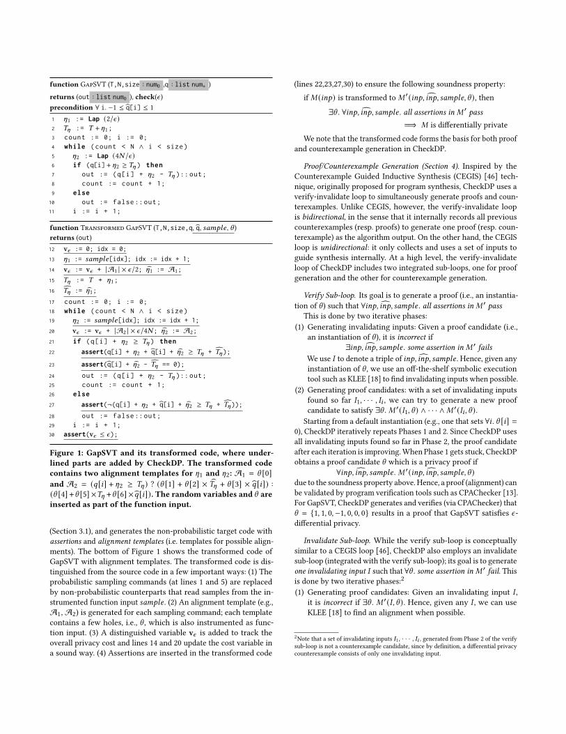
Counterexample Generation. This component takes an invalidat-ing input 𝐼𝑖 and then tries to find an alignment\𝑖 such that𝑀 ′(𝐼𝑖 , \𝑖 )(meaning that 𝐼𝑖 is not a counterexample since it can be aligned by\𝑖 ). For example, consider a corner case in Figure 5a, where ProofGeneration fails to find a common proof of both 𝐼0 and 𝐼1, but eachof 𝐼0 and 𝐼1 has a proof (illustrated by the two solid circles aroundthem). Mostly likely, this occurs when the program being analyzedis incorrect (hence, no common proof) but neither 𝐼1 nor 𝐼2 is agood candidate for counterexample of differential privacy, sinceeach of them can be aligned in isolation.

Restart. This component is symmetric to the Invalidating InputGeneration component in the verify sub-loop: it takes all previouslyfound proof candidates \1, · · · , \𝑖 and tries to find an invalidatinginput 𝐼𝑖+1 such that: ¬𝑀 ′(𝐼𝑖+1, \1) ∧ · · · ¬𝑀 ′(𝐼𝑖+1, \𝑖 ) .

If found, 𝐼𝑖+1 will intuitively be out of scope of all found proofsand serve as a “better” invalidating input. In theory, we can closethe invalidate sub-loop by feeding 𝐼𝑖+1 back to CounterexampleGeneration. However, doing sowill make proof and counterexamplegeneration isolated tasks. Instead, we take an integrated approach,which we discuss shortly, where the verify and invalidate sub-loopscommunicate to generate proofs and counterexamples in a moreefficient and simultaneous way.

Exit Edges. If no \ is found to prove 𝐼𝑖 = (𝑖𝑛𝑝, inp, 𝑠𝑎𝑚𝑝𝑙𝑒), acounterexample 𝐶 = (𝑖𝑛𝑝, 𝑖𝑛𝑝 + 𝑖𝑛𝑝,𝑀 ′(𝑖𝑛𝑝, 𝑖𝑛𝑝, 𝑠𝑎𝑚𝑝𝑙𝑒, \0)) canbe formed and sent to an external exact probabilistic solver PSI [33]for validation. In theory, the Restart component might fail to find anew invalidating input given \1, · · · , \𝑖 . However, this “unknown”state never showed up in our experience.

4.3 Integrating Verify and Invalidate Sub-LoopsWe integrate the verify and invalidate sub-loops as follows: follow-ing the “Invalidate Sub-loop” edge of the Proof Generation com-ponent, the latest invalidating input 𝐼𝑖 (i.e., the “best” invalidatinginput so far) is passed to the Counterexample Generation compo-nent to start the invalidate sub-loop. Moreover, the newly generatedinvalidating input 𝐼𝑖 from the Restart component is fed back to theProof Generation component to start the verify sub-loop.

We note that by the design of the verify-invalidate loop, it alter-natively runs Invalidating Input Generation and Proof Generationcomponents. By doing so, the proof keeps improving while the in-validating inputs are getting closer to a true counterexample (sincethe most recent one violates a “better” proof). More intuitively,consider an invalidating input 𝐼0 as a point in the entire input space,illustrated in Figure 5b. A proof candidate \1 is able to prove thealgorithm for a subset of inputs including 𝐼0 (indicated by the circlearound 𝐼0). The Invalidating Input Generation component then triesto find another invalidating 𝐼1 that violates \1 (falls outside of the\1 circle). Next, the Proof Generation component finds better proofcandidate \2 which proves (“covers”) both 𝐼0 and 𝐼1.

We also note that it is crucial to consider all invalidating inputsso far rather than the last input 𝐼𝑖 in the Proof Generation compo-nent: the efficiency of our approach crucially relies on “improving”

the proofs quantified by validating more invalidating inputs. With-out the improving proofs, the iterative procedure might fail toterminate in case shown in Figure 5a: the procedure might repeat𝐼0, \1, 𝐼1, \2, 𝐼0, \1, · · · . This is confirmed in our empirical study.

Unknown State. Due to the soundness result (Theorem 3), theprogram being analyzed is verified whenever CheckDP returns witha proof. Moreover, a validated counterexample by PSI disprovesan incorrect mechanism. However, two reasons might lead to the“unknown” state in the Figure 4: the generated counterexampleis invalid or the Restart component fails to find a new invalidat-ing input. However, for all the correct and incorrect examples weexplored, the unknown state never showed up.

5 IMPLEMENTATION AND EVALUATIONWe implemented CheckDP in Python3. The Program Transforma-tion phase is implemented as a trans-compiler from CheckDP code(Figure 2) to C code. Following the transformation rules in Fig-ure 3, the trans-compiler tracks the typing environment, gathersthe needed constraints for the expressions, and more importantly,instruments corresponding statements when appropriate. More-over, it adds a final assertion assert(v𝜖 ≤ 𝜖𝑏 ) before each returncommand, where 𝜖𝑏 is the annotated privacy bound to be checked.Once all assertions are generated, the trans-compiler generates onealignment template for each sampling instruction as described inAlgorithm 1. For the Proof and Counterexample Generation phase(i.e., verify-invalidate loop in Section 4), we used an efficient sym-bolic executor KLEE [18] for most tasks. Due to limited support ofunbounded lists in KLEE, we fix the length of lists to be 5 in ourevaluation. Also, to speed up the search, KLEE is configured to exitonce an assertion is hit. We note that the use of KLEE is to discoveralignments and counterexamples, where alignments are eventu-ally verified by our sound Verifier component with arbitrary arraylength; counterexamples are confirmed by PSI. Moreover, CheckDPautomatically extends the array length until either a verified proofor verified counterexample is produced.

Finally, we deploy a verification tool CPAChecker [13] for theVerifier component in CheckDP, which is capable of automaticallyverifying C programs with given configuration (predicateAnalysisis used). Note that CPAChecker is able to generate counterexam-ples for a failed verification. If the verification fails (which did nothappen in our evaluation), CheckDP can feed the counterexampleback to the Proof and Counterexample Generation component.

5.1 Case StudiesAside from GapSVT, we also evaluate CheckDP on the standardbenchmark used in previous mechanism verifiers [3, 51, 52] andcounterexample generators [14, 23],4 including correct ones such asNumSVT, PartialSum, and SmartSum, as well as the incorrect vari-ants of SVT reported in [40] and BadPartialSum. To show the powerof CheckDP and expressiveness of our template generation algo-rithm, we also evaluate on a couple of correct/incorrect mechanismsthat, to the best of our knowledge, have not been proved/disproved

3Publically available at https://github.com/cmla-psu/checkdp.4We note that like all tools designed for privacy mechanisms (e.g., [3, 14, 23, 51, 52]),the benchmark do not include iterative programs that are built on those privacymechanisms, such as k-means clustering, k-medians, since they are out of scope.

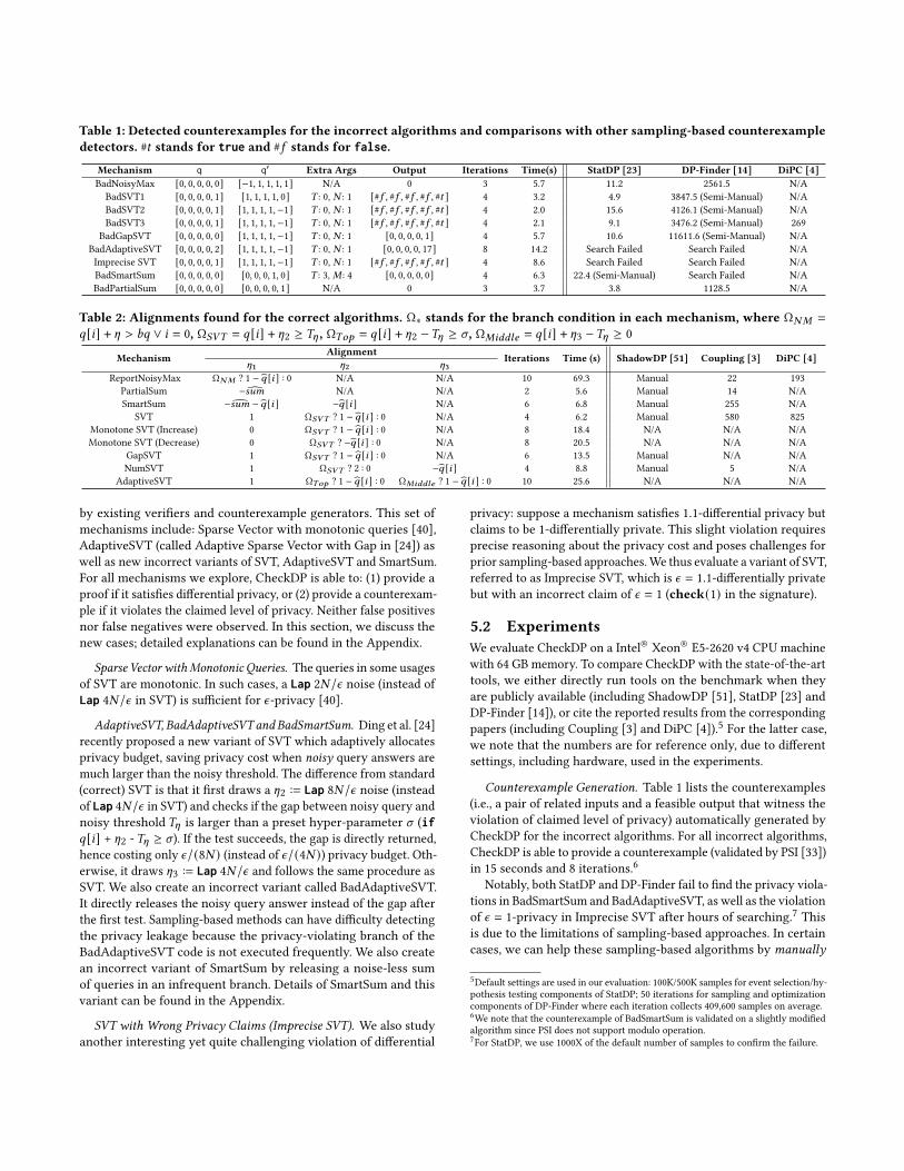
Table 1: Detected counterexamples for the incorrect algorithms and comparisons with other sampling-based counterexampledetectors. #𝑡 stands for true and #𝑓 stands for false.

Mechanism q q′ Extra Args Output Iterations Time(s) StatDP [23] DP-Finder [14] DiPC [4]BadNoisyMax [0, 0, 0, 0, 0] [−1, 1, 1, 1, 1] N/A 0 3 5.7 11.2 2561.5 N/ABadSVT1 [0, 0, 0, 0, 1] [1, 1, 1, 1, 0] 𝑇 : 0, 𝑁 : 1 [#𝑓 , #𝑓 , #𝑓 , #𝑓 , #𝑡 ] 4 3.2 4.9 3847.5 (Semi-Manual) N/ABadSVT2 [0, 0, 0, 0, 1] [1, 1, 1, 1,−1] 𝑇 : 0, 𝑁 : 1 [#𝑓 , #𝑓 , #𝑓 , #𝑓 , #𝑡 ] 4 2.0 15.6 4126.1 (Semi-Manual) N/ABadSVT3 [0, 0, 0, 0, 1] [1, 1, 1, 1,−1] 𝑇 : 0, 𝑁 : 1 [#𝑓 , #𝑓 , #𝑓 , #𝑓 , #𝑡 ] 4 2.1 9.1 3476.2 (Semi-Manual) 269

BadGapSVT [0, 0, 0, 0, 0] [1, 1, 1, 1,−1] 𝑇 : 0, 𝑁 : 1 [0, 0, 0, 0, 1] 4 5.7 10.6 11611.6 (Semi-Manual) N/ABadAdaptiveSVT [0, 0, 0, 0, 2] [1, 1, 1, 1,−1] 𝑇 : 0, 𝑁 : 1 [0, 0, 0, 0, 17] 8 14.2 Search Failed Search Failed N/AImprecise SVT [0, 0, 0, 0, 1] [1, 1, 1, 1,−1] 𝑇 : 0, 𝑁 : 1 [#𝑓 , #𝑓 , #𝑓 , #𝑓 , #𝑡 ] 4 8.6 Search Failed Search Failed N/ABadSmartSum [0, 0, 0, 0, 0] [0, 0, 0, 1, 0] 𝑇 : 3,𝑀 : 4 [0, 0, 0, 0, 0] 4 6.3 22.4 (Semi-Manual) Search Failed N/ABadPartialSum [0, 0, 0, 0, 0] [0, 0, 0, 0, 1] N/A 0 3 3.7 3.8 1128.5 N/A

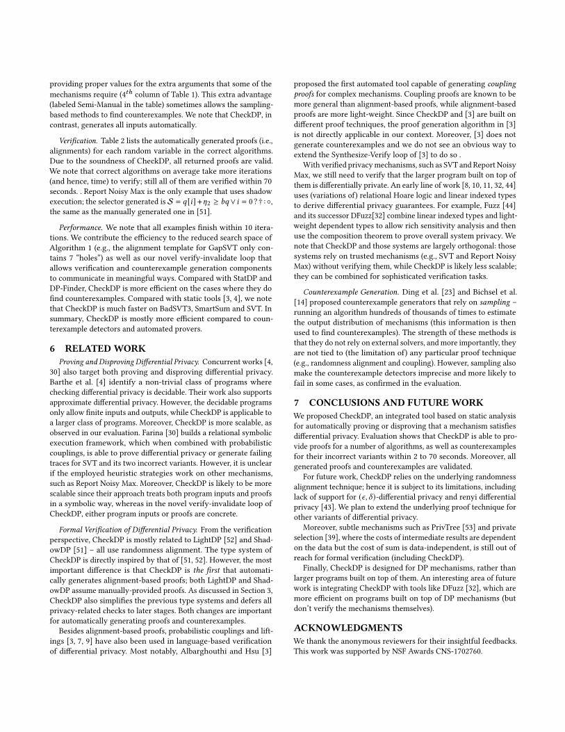
Table 2: Alignments found for the correct algorithms. Ω∗ stands for the branch condition in each mechanism, where Ω𝑁𝑀 =

𝑞 [𝑖] + [ > 𝑏𝑞 ∨ 𝑖 = 0, Ω𝑆𝑉𝑇 = 𝑞 [𝑖] + [2 ≥ 𝑇[ , Ω𝑇𝑜𝑝 = 𝑞 [𝑖] + [2 −𝑇[ ≥ 𝜎 , Ω𝑀𝑖𝑑𝑑𝑙𝑒 = 𝑞 [𝑖] + [3 −𝑇[ ≥ 0

Mechanism Alignment Iterations Time (s) ShadowDP [51] Coupling [3] DiPC [4][1 [2 [3

ReportNoisyMax Ω𝑁𝑀 ? 1 − �� [𝑖 ] : 0 N/A N/A 10 69.3 Manual 22 193PartialSum −𝑠𝑢𝑚 N/A N/A 2 5.6 Manual 14 N/ASmartSum −𝑠𝑢𝑚 − �� [𝑖 ] −�� [𝑖 ] N/A 6 6.8 Manual 255 N/A

SVT 1 Ω𝑆𝑉𝑇 ? 1 − �� [𝑖 ] : 0 N/A 4 6.2 Manual 580 825Monotone SVT (Increase) 0 Ω𝑆𝑉𝑇 ? 1 − �� [𝑖 ] : 0 N/A 8 18.4 N/A N/A N/AMonotone SVT (Decrease) 0 Ω𝑆𝑉𝑇 ? −�� [𝑖 ] : 0 N/A 8 20.5 N/A N/A N/A

GapSVT 1 Ω𝑆𝑉𝑇 ? 1 − �� [𝑖 ] : 0 N/A 6 13.5 Manual N/A N/ANumSVT 1 Ω𝑆𝑉𝑇 ? 2 : 0 −�� [𝑖 ] 4 8.8 Manual 5 N/A

AdaptiveSVT 1 Ω𝑇𝑜𝑝 ? 1 − �� [𝑖 ] : 0 Ω𝑀𝑖𝑑𝑑𝑙𝑒 ? 1 − �� [𝑖 ] : 0 10 25.6 N/A N/A N/A

by existing verifiers and counterexample generators. This set ofmechanisms include: Sparse Vector with monotonic queries [40],AdaptiveSVT (called Adaptive Sparse Vector with Gap in [24]) aswell as new incorrect variants of SVT, AdaptiveSVT and SmartSum.For all mechanisms we explore, CheckDP is able to: (1) provide aproof if it satisfies differential privacy, or (2) provide a counterexam-ple if it violates the claimed level of privacy. Neither false positivesnor false negatives were observed. In this section, we discuss thenew cases; detailed explanations can be found in the Appendix.

Sparse Vector with Monotonic Queries. The queries in some usagesof SVT are monotonic. In such cases, a Lap 2𝑁 /𝜖 noise (instead ofLap 4𝑁 /𝜖 in SVT) is sufficient for 𝜖-privacy [40].

AdaptiveSVT, BadAdaptiveSVT and BadSmartSum. Ding et al. [24]recently proposed a new variant of SVT which adaptively allocatesprivacy budget, saving privacy cost when noisy query answers aremuch larger than the noisy threshold. The difference from standard(correct) SVT is that it first draws a [2 := Lap 8𝑁 /𝜖 noise (insteadof Lap 4𝑁 /𝜖 in SVT) and checks if the gap between noisy query andnoisy threshold 𝑇[ is larger than a preset hyper-parameter 𝜎 (if𝑞 [𝑖] + [2 -𝑇[ ≥ 𝜎). If the test succeeds, the gap is directly returned,hence costing only 𝜖/(8𝑁 ) (instead of 𝜖/(4𝑁 )) privacy budget. Oth-erwise, it draws [3 := Lap 4𝑁 /𝜖 and follows the same procedure asSVT. We also create an incorrect variant called BadAdaptiveSVT.It directly releases the noisy query answer instead of the gap afterthe first test. Sampling-based methods can have difficulty detectingthe privacy leakage because the privacy-violating branch of theBadAdaptiveSVT code is not executed frequently. We also createan incorrect variant of SmartSum by releasing a noise-less sumof queries in an infrequent branch. Details of SmartSum and thisvariant can be found in the Appendix.

SVT with Wrong Privacy Claims (Imprecise SVT). We also studyanother interesting yet quite challenging violation of differential

privacy: suppose a mechanism satisfies 1.1-differential privacy butclaims to be 1-differentially private. This slight violation requiresprecise reasoning about the privacy cost and poses challenges forprior sampling-based approaches.We thus evaluate a variant of SVT,referred to as Imprecise SVT, which is 𝜖 = 1.1-differentially privatebut with an incorrect claim of 𝜖 = 1 (check(1) in the signature).

5.2 ExperimentsWe evaluate CheckDP on a Intel® Xeon® E5-2620 v4 CPU machinewith 64 GB memory. To compare CheckDP with the state-of-the-arttools, we either directly run tools on the benchmark when theyare publicly available (including ShadowDP [51], StatDP [23] andDP-Finder [14]), or cite the reported results from the correspondingpapers (including Coupling [3] and DiPC [4]).5 For the latter case,we note that the numbers are for reference only, due to differentsettings, including hardware, used in the experiments.

Counterexample Generation. Table 1 lists the counterexamples(i.e., a pair of related inputs and a feasible output that witness theviolation of claimed level of privacy) automatically generated byCheckDP for the incorrect algorithms. For all incorrect algorithms,CheckDP is able to provide a counterexample (validated by PSI [33])in 15 seconds and 8 iterations.6

Notably, both StatDP and DP-Finder fail to find the privacy viola-tions in BadSmartSum and BadAdaptiveSVT, as well as the violationof 𝜖 = 1-privacy in Imprecise SVT after hours of searching.7 Thisis due to the limitations of sampling-based approaches. In certaincases, we can help these sampling-based algorithms by manually

5Default settings are used in our evaluation: 100K/500K samples for event selection/hy-pothesis testing components of StatDP; 50 iterations for sampling and optimizationcomponents of DP-Finder where each iteration collects 409,600 samples on average.6We note that the counterexample of BadSmartSum is validated on a slightly modifiedalgorithm since PSI does not support modulo operation.7For StatDP, we use 1000X of the default number of samples to confirm the failure.

providing proper values for the extra arguments that some of themechanisms require (4𝑡ℎ column of Table 1). This extra advantage(labeled Semi-Manual in the table) sometimes allows the sampling-based methods to find counterexamples. We note that CheckDP, incontrast, generates all inputs automatically.

Verification. Table 2 lists the automatically generated proofs (i.e.,alignments) for each random variable in the correct algorithms.Due to the soundness of CheckDP, all returned proofs are valid.We note that correct algorithms on average take more iterations(and hence, time) to verify; still all of them are verified within 70seconds. . Report Noisy Max is the only example that uses shadowexecution; the selector generated is S = 𝑞 [𝑖] +[2 ≥ 𝑏𝑞∨ 𝑖 = 0?† :◦,the same as the manually generated one in [51].

Performance. We note that all examples finish within 10 itera-tions. We contribute the efficiency to the reduced search space ofAlgorithm 1 (e.g., the alignment template for GapSVT only con-tains 7 “holes”) as well as our novel verify-invalidate loop thatallows verification and counterexample generation componentsto communicate in meaningful ways. Compared with StatDP andDP-Finder, CheckDP is more efficient on the cases where they dofind counterexamples. Compared with static tools [3, 4], we notethat CheckDP is much faster on BadSVT3, SmartSum and SVT. Insummary, CheckDP is mostly more efficient compared to coun-terexample detectors and automated provers.

6 RELATEDWORKProving and Disproving Differential Privacy. Concurrent works [4,

30] also target both proving and disproving differential privacy.Barthe et al. [4] identify a non-trivial class of programs wherechecking differential privacy is decidable. Their work also supportsapproximate differential privacy. However, the decidable programsonly allow finite inputs and outputs, while CheckDP is applicable toa larger class of programs. Moreover, CheckDP is more scalable, asobserved in our evaluation. Farina [30] builds a relational symbolicexecution framework, which when combined with probabilisticcouplings, is able to prove differential privacy or generate failingtraces for SVT and its two incorrect variants. However, it is unclearif the employed heuristic strategies work on other mechanisms,such as Report Noisy Max. Moreover, CheckDP is likely to be morescalable since their approach treats both program inputs and proofsin a symbolic way, whereas in the novel verify-invalidate loop ofCheckDP, either program inputs or proofs are concrete.

Formal Verification of Differential Privacy. From the verificationperspective, CheckDP is mostly related to LightDP [52] and Shad-owDP [51] – all use randomness alignment. The type system ofCheckDP is directly inspired by that of [51, 52]. However, the mostimportant difference is that CheckDP is the first that automati-cally generates alignment-based proofs; both LightDP and Shad-owDP assume manually-provided proofs. As discussed in Section 3,CheckDP also simplifies the previous type systems and defers allprivacy-related checks to later stages. Both changes are importantfor automatically generating proofs and counterexamples.

Besides alignment-based proofs, probabilistic couplings and lift-ings [3, 7, 9] have also been used in language-based verificationof differential privacy. Most notably, Albarghouthi and Hsu [3]

proposed the first automated tool capable of generating couplingproofs for complex mechanisms. Coupling proofs are known to bemore general than alignment-based proofs, while alignment-basedproofs are more light-weight. Since CheckDP and [3] are built ondifferent proof techniques, the proof generation algorithm in [3]is not directly applicable in our context. Moreover, [3] does notgenerate counterexamples and we do not see an obvious way toextend the Synthesize-Verify loop of [3] to do so .

With verified privacymechanisms, such as SVT and Report NoisyMax, we still need to verify that the larger program built on top ofthem is differentially private. An early line of work [8, 10, 11, 32, 44]uses (variations of) relational Hoare logic and linear indexed typesto derive differential privacy guarantees. For example, Fuzz [44]and its successor DFuzz[32] combine linear indexed types and light-weight dependent types to allow rich sensitivity analysis and thenuse the composition theorem to prove overall system privacy. Wenote that CheckDP and those systems are largely orthogonal: thosesystems rely on trusted mechanisms (e.g., SVT and Report NoisyMax) without verifying them, while CheckDP is likely less scalable;they can be combined for sophisticated verification tasks.

Counterexample Generation. Ding et al. [23] and Bichsel et al.[14] proposed counterexample generators that rely on sampling –running an algorithm hundreds of thousands of times to estimatethe output distribution of mechanisms (this information is thenused to find counterexamples). The strength of these methods isthat they do not rely on external solvers, andmore importantly, theyare not tied to (the limitation of) any particular proof technique(e.g., randomness alignment and coupling). However, sampling alsomake the counterexample detectors imprecise and more likely tofail in some cases, as confirmed in the evaluation.

7 CONCLUSIONS AND FUTUREWORKWe proposed CheckDP, an integrated tool based on static analysisfor automatically proving or disproving that a mechanism satisfiesdifferential privacy. Evaluation shows that CheckDP is able to pro-vide proofs for a number of algorithms, as well as counterexamplesfor their incorrect variants within 2 to 70 seconds. Moreover, allgenerated proofs and counterexamples are validated.

For future work, CheckDP relies on the underlying randomnessalignment technique; hence it is subject to its limitations, includinglack of support for (𝜖, 𝛿)-differential privacy and renyi differentialprivacy [43]. We plan to extend the underlying proof technique forother variants of differential privacy.

Moreover, subtle mechanisms such as PrivTree [53] and privateselection [39], where the costs of intermediate results are dependenton the data but the cost of sum is data-independent, is still out ofreach for formal verification (including CheckDP).

Finally, CheckDP is designed for DP mechanisms, rather thanlarger programs built on top of them. An interesting area of futurework is integrating CheckDP with tools like DFuzz [32], which aremore efficient on programs built on top of DP mechanisms (butdon’t verify the mechanisms themselves).

ACKNOWLEDGMENTSWe thank the anonymous reviewers for their insightful feedbacks.This work was supported by NSF Awards CNS-1702760.

REFERENCES[1] John M. Abowd. 2018. The U.S. Census Bureau Adopts Differential Privacy.

In Proceedings of the 24th ACM SIGKDD International Conference on KnowledgeDiscovery and Data Mining (London, United Kingdom) (KDD ’18). ACM, NewYork, NY, USA, 2867–2867.

[2] Alfred V Aho, Ravi Sethi, and Jeffrey D Ullman. 1986. Compilers, principles,techniques. Addison wesley 7, 8 (1986), 9.

[3] Aws Albarghouthi and Justin Hsu. 2017. Synthesizing Coupling Proofs of Differ-ential Privacy. Proceedings of ACM Programming Languages 2, POPL, Article 58(Dec. 2017), 30 pages.

[4] Gilles Barthe, Rohit Chadha, Vishal Jagannath, A. Prasad Sistla, and MaheshViswanathan. 2020. Deciding Differential Privacy for Programs with FiniteInputs and Outputs. In Proceedings of the 35th Annual ACM/IEEE Symposium onLogic in Computer Science (Saarbrücken, Germany) (LICS ’20). Association forComputing Machinery, New York, NY, USA, 141–154. https://doi.org/10.1145/3373718.3394796

[5] Gilles Barthe, George Danezis, Benjamin Gregoire, Cesar Kunz, and SantiagoZanella-Beguelin. 2013. Verified Computational Differential Privacy with Appli-cations to Smart Metering. In Proceedings of the 2013 IEEE 26th Computer SecurityFoundations Symposium (CSF ’13). IEEE Computer Society, Washington, DC, USA,287–301.

[6] Gilles Barthe, Pedro R. D’Argenio, and Tamara Rezk. 2004. Secure InformationFlow by Self-Composition. In Proceedings of the 17th IEEE Workshop on ComputerSecurity Foundations (CSFW ’04). IEEE Computer Society, Washington, DC, USA,100–.

[7] Gilles Barthe, Noémie Fong, Marco Gaboardi, Benjamin Grégoire, Justin Hsu,and Pierre-Yves Strub. 2016. Advanced Probabilistic Couplings for DifferentialPrivacy. In Proceedings of the 2016 ACM SIGSAC Conference on Computer andCommunications Security (Vienna, Austria) (CCS ’16). ACM, New York, NY, USA,55–67.

[8] Gilles Barthe, Marco Gaboardi, Emilio Jesús Gallego Arias, Justin Hsu, CésarKunz, and Pierre-Yves Strub. 2014. Proving Differential Privacy in Hoare Logic.In Proceedings of the 2014 IEEE 27th Computer Security Foundations Symposium(CSF ’14). IEEE Computer Society, Washington, DC, USA, 411–424.

[9] Gilles Barthe, Marco Gaboardi, Benjamin Grégoire, Justin Hsu, and Pierre-YvesStrub. 2016. Proving Differential Privacy via Probabilistic Couplings. In Proceed-ings of the 31st Annual ACM/IEEE Symposium on Logic in Computer Science (NewYork, NY, USA) (LICS ’16). ACM, New York, NY, USA, 749–758.

[10] Gilles Barthe, Boris Köpf, Federico Olmedo, and Santiago Zanella Béguelin. 2012.Probabilistic Relational Reasoning for Differential Privacy. In Proceedings of the39th Annual ACM SIGPLAN-SIGACT Symposium on Principles of ProgrammingLanguages (Philadelphia, PA, USA) (POPL ’12). ACM, New York, NY, USA, 97–110.

[11] Gilles Barthe and Federico Olmedo. 2013. Beyond Differential Privacy: Compo-sition Theorems and Relational Logic for f-divergences Between ProbabilisticPrograms. In Proceedings of the 40th International Conference on Automata, Lan-guages, and Programming - Volume Part II (Riga, Latvia) (ICALP’13). Springer-Verlag, Berlin, Heidelberg, 49–60.

[12] Jean-Francois Bergeretti and Bernard A. Carré. 1985. Information-flow and Data-flow Analysis of While-programs. ACM Trans. Program. Lang. Syst. 7, 1 (Jan.1985), 37–61. https://doi.org/10.1145/2363.2366

[13] Dirk Beyer and M. Erkan Keremoglu. 2011. CPACHECKER: A Tool for Config-urable Software Verification. In Proceedings of the 23rd International Conferenceon Computer Aided Verification (Snowbird, UT) (CAV’11). Springer-Verlag, Berlin,Heidelberg, 184–190.

[14] Benjamin Bichsel, TimonGehr, DanaDrachsler-Cohen, Petar Tsankov, andMartinVechev. 2018. DP-Finder: Finding Differential Privacy Violations by Sampling andOptimization. In Proceedings of the 2018 ACM SIGSAC Conference on Computerand Communications Security (Toronto, Canada) (CCS ’18). ACM, New York, NY,USA, 508–524.

[15] Andrea Bittau, Úlfar Erlingsson, Petros Maniatis, Ilya Mironov, Ananth Raghu-nathan, David Lie, Mitch Rudominer, Ushasree Kode, Julien Tinnes, and BernhardSeefeld. 2017. Prochlo: Strong Privacy for Analytics in the Crowd. In Proceedingsof the 26th Symposium on Operating Systems Principles (Shanghai, China) (SOSP’17). ACM, New York, NY, USA, 441–459. https://doi.org/10.1145/3132747.3132769

[16] Mark Bun and Thomas Steinke. 2016. Concentrated Differential Privacy: Sim-plifications, Extensions, and Lower Bounds. In Proceedings, Part I, of the 14thInternational Conference on Theory of Cryptography - Volume 9985. Springer-VerlagNew York, Inc., New York, NY, USA, 635–658.

[17] U. S. Census Bureau. 2019. On The Map: Longitudinal Employer-HouseholdDynamics. https://lehd.ces.census.gov/applications/help/onthemap.html#!confidentiality_protection

[18] Cristian Cadar, Daniel Dunbar, and Dawson Engler. 2008. KLEE: Unassisted andAutomatic Generation of High-coverage Tests for Complex Systems Programs.In Proceedings of the 8th USENIX Conference on Operating Systems Design andImplementation (San Diego, California) (OSDI’08). USENIX Association, Berkeley,CA, USA, 209–224. http://dl.acm.org/citation.cfm?id=1855741.1855756

[19] T.-H. Hubert Chan, Elaine Shi, and Dawn Song. 2011. Private and ContinualRelease of Statistics. ACM Trans. Inf. Syst. Secur. 14, 3, Article 26 (Nov. 2011),

24 pages.[20] Rui Chen, Qian Xiao, Yu Zhang, and Jianliang Xu. 2015. Differentially Private

High-Dimensional Data Publication via Sampling-Based Inference. In Proceedingsof the 21th ACM SIGKDD International Conference on Knowledge Discovery andData Mining (Sydney, NSW, Australia) (KDD ’15). ACM, New York, NY, USA,129–138. https://doi.org/10.1145/2783258.2783379

[21] Yan Chen and Ashwin Machanavajjhala. 2015. On the Privacy Properties ofVariants on the Sparse Vector Technique. http://arxiv.org/abs/1508.07306.

[22] Bolin Ding, Janardhan Kulkarni, and Sergey Yekhanin. 2017. Collecting TelemetryData Privately. In Proceedings of the 31st International Conference on NeuralInformation Processing Systems (Long Beach, California, USA) (NIPS’17). CurranAssociates Inc., USA, 3574–3583. http://dl.acm.org/citation.cfm?id=3294996.3295115

[23] Zeyu Ding, Yuxin Wang, Guanhong Wang, Danfeng Zhang, and Daniel Kifer.2018. Detecting Violations of Differential Privacy. In Proceedings of the 2018 ACMSIGSAC Conference on Computer and Communications Security (Toronto, Canada)(CCS ’18). ACM, New York, NY, USA, 475–489.

[24] Zeyu Ding, Yuxin Wang, Danfeng Zhang, and Daniel Kifer. 2019. Free Gap Infor-mation from the Differentially Private Sparse Vector and Noisy Max Mechanisms.PVLDB 13, 3 (2019), 293–306. https://doi.org/10.14778/3368289.3368295

[25] Cynthia Dwork. 2006. Differential Privacy. In Proceedings of the 33rd InternationalConference on Automata, Languages and Programming - Volume Part II (Venice,Italy) (ICALP’06). Springer-Verlag, Berlin, Heidelberg, 1–12. https://doi.org/10.1007/11787006_1

[26] Cynthia Dwork, Krishnaram Kenthapadi, Frank McSherry, Ilya Mironov, andMoni Naor. 2006. Our Data, Ourselves: Privacy via Distributed Noise Generation.In Proceedings of the 24th Annual International Conference on The Theory andApplications of Cryptographic Techniques (St. Petersburg, Russia) (EUROCRYPT’06).Springer-Verlag, Berlin, Heidelberg, 486–503.

[27] Cynthia Dwork, Frank McSherry, Kobbi Nissim, and Adam Smith. 2006. Cali-brating Noise to Sensitivity in Private Data Analysis. In Theory of Cryptography,Shai Halevi and Tal Rabin (Eds.). Springer Berlin Heidelberg, Berlin, Heidelberg,265–284.

[28] Cynthia Dwork, Aaron Roth, et al. 2014. The algorithmic foundations of differ-ential privacy. Theoretical Computer Science 9, 3–4 (2014), 211–407.

[29] Úlfar Erlingsson, Vasyl Pihur, and Aleksandra Korolova. 2014. RAPPOR: Ran-domized Aggregatable Privacy-Preserving Ordinal Response. In Proceedings ofthe 2014 ACM SIGSAC Conference on Computer and Communications Security(Scottsdale, Arizona, USA) (CCS ’14). ACM, New York, NY, USA, 1054–1067.

[30] Gian Pietro Farina. 2020. Coupled Relational Symbolic Execution. Ph.D. Disserta-tion. State University of New York at Buffalo.

[31] Jeanne Ferrante, Karl J Ottenstein, and Joe D Warren. 1987. The program de-pendence graph and its use in optimization. ACM Transactions on ProgrammingLanguages and Systems (TOPLAS) 9, 3 (1987), 319–349.

[32] Marco Gaboardi, Andreas Haeberlen, Justin Hsu, Arjun Narayan, and Benjamin C.Pierce. 2013. Linear Dependent Types for Differential Privacy. In Proceedings ofthe 40th Annual ACM SIGPLAN-SIGACT Symposium on Principles of ProgrammingLanguages (Rome, Italy) (POPL ’13). ACM, New York, NY, USA, 357–370. https://doi.org/10.1145/2429069.2429113

[33] Timon Gehr, Sasa Misailovic, and Martin Vechev. 2016. PSI: Exact SymbolicInference for Probabilistic Programs. In Computer Aided Verification, SwaratChaudhuri and Azadeh Farzan (Eds.). Springer International Publishing, Cham,62–83.

[34] Anna Gilbert and Audra McMillan. 2018. Property Testing for Differential Privacy.arXiv:1806.06427 [cs.CR]

[35] Samuel Haney, Ashwin Machanavajjhala, John M. Abowd, Matthew Graham,Mark Kutzbach, and Lars Vilhuber. 2017. Utility Cost of Formal Privacy forReleasing National Employer-Employee Statistics. In Proceedings of the 2017ACM International Conference on Management of Data (Chicago, Illinois, USA)(SIGMOD ’17). ACM, New York, NY, USA, 1339–1354. https://doi.org/10.1145/3035918.3035940

[36] Noah Johnson, Joseph PNear, andDawn Song. 2018. Towards practical differentialprivacy for SQL queries. Proceedings of the VLDB Endowment 11, 5 (2018), 526–539.

[37] Dexter Kozen. 1981. Semantics of probabilistic programs. J. Comput. System Sci.22, 3 (1981), 328 – 350.

[38] Jaewoo Lee and Christopher W. Clifton. 2014. Top-k Frequent Itemsets via Dif-ferentially Private FP-trees. In Proceedings of the 20th ACM SIGKDD InternationalConference on Knowledge Discovery and Data Mining (New York, New York, USA)(KDD ’14). ACM, New York, NY, USA, 931–940. https://doi.org/10.1145/2623330.2623723

[39] Jingcheng Liu and Kunal Talwar. 2019. Private Selection from Private Candidates.In Proceedings of the 51st Annual ACM SIGACT Symposium on Theory of Computing(Phoenix, AZ, USA) (STOC 2019). Association for Computing Machinery, NewYork, NY, USA, 298–309. https://doi.org/10.1145/3313276.3316377

[40] Min Lyu, Dong Su, and Ninghui Li. 2017. Understanding the sparse vectortechnique for differential privacy. Proceedings of the VLDB Endowment 10, 6(2017), 637–648.

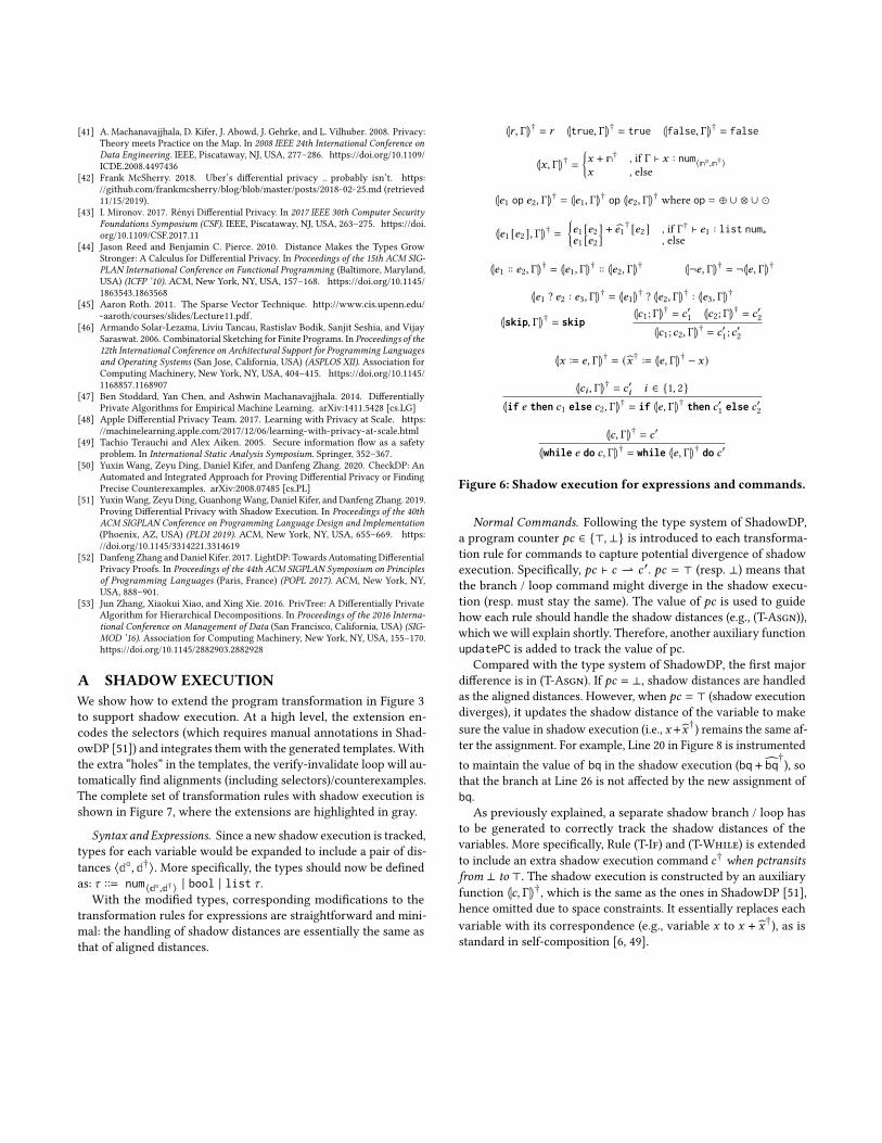
[41] A. Machanavajjhala, D. Kifer, J. Abowd, J. Gehrke, and L. Vilhuber. 2008. Privacy:Theory meets Practice on the Map. In 2008 IEEE 24th International Conference onData Engineering. IEEE, Piscataway, NJ, USA, 277–286. https://doi.org/10.1109/ICDE.2008.4497436

[42] Frank McSherry. 2018. Uber’s differential privacy .. probably isn’t. https://github.com/frankmcsherry/blog/blob/master/posts/2018-02-25.md (retrieved11/15/2019).

[43] I. Mironov. 2017. Rényi Differential Privacy. In 2017 IEEE 30th Computer SecurityFoundations Symposium (CSF). IEEE, Piscataway, NJ, USA, 263–275. https://doi.org/10.1109/CSF.2017.11

[44] Jason Reed and Benjamin C. Pierce. 2010. Distance Makes the Types GrowStronger: A Calculus for Differential Privacy. In Proceedings of the 15th ACM SIG-PLAN International Conference on Functional Programming (Baltimore, Maryland,USA) (ICFP ’10). ACM, New York, NY, USA, 157–168. https://doi.org/10.1145/1863543.1863568

[45] Aaron Roth. 2011. The Sparse Vector Technique. http://www.cis.upenn.edu/~aaroth/courses/slides/Lecture11.pdf.

[46] Armando Solar-Lezama, Liviu Tancau, Rastislav Bodik, Sanjit Seshia, and VijaySaraswat. 2006. Combinatorial Sketching for Finite Programs. In Proceedings of the12th International Conference on Architectural Support for Programming Languagesand Operating Systems (San Jose, California, USA) (ASPLOS XII). Association forComputing Machinery, New York, NY, USA, 404–415. https://doi.org/10.1145/1168857.1168907

[47] Ben Stoddard, Yan Chen, and Ashwin Machanavajjhala. 2014. DifferentiallyPrivate Algorithms for Empirical Machine Learning. arXiv:1411.5428 [cs.LG]

[48] Apple Differential Privacy Team. 2017. Learning with Privacy at Scale. https://machinelearning.apple.com/2017/12/06/learning-with-privacy-at-scale.html

[49] Tachio Terauchi and Alex Aiken. 2005. Secure information flow as a safetyproblem. In International Static Analysis Symposium. Springer, 352–367.

[50] Yuxin Wang, Zeyu Ding, Daniel Kifer, and Danfeng Zhang. 2020. CheckDP: AnAutomated and Integrated Approach for Proving Differential Privacy or FindingPrecise Counterexamples. arXiv:2008.07485 [cs.PL]

[51] YuxinWang, Zeyu Ding, GuanhongWang, Daniel Kifer, and Danfeng Zhang. 2019.Proving Differential Privacy with Shadow Execution. In Proceedings of the 40thACM SIGPLAN Conference on Programming Language Design and Implementation(Phoenix, AZ, USA) (PLDI 2019). ACM, New York, NY, USA, 655–669. https://doi.org/10.1145/3314221.3314619

[52] Danfeng Zhang andDaniel Kifer. 2017. LightDP: Towards AutomatingDifferentialPrivacy Proofs. In Proceedings of the 44th ACM SIGPLAN Symposium on Principlesof Programming Languages (Paris, France) (POPL 2017). ACM, New York, NY,USA, 888–901.

[53] Jun Zhang, Xiaokui Xiao, and Xing Xie. 2016. PrivTree: A Differentially PrivateAlgorithm for Hierarchical Decompositions. In Proceedings of the 2016 Interna-tional Conference on Management of Data (San Francisco, California, USA) (SIG-MOD ’16). Association for Computing Machinery, New York, NY, USA, 155–170.https://doi.org/10.1145/2882903.2882928

A SHADOW EXECUTIONWe show how to extend the program transformation in Figure 3to support shadow execution. At a high level, the extension en-codes the selectors (which requires manual annotations in Shad-owDP [51]) and integrates themwith the generated templates. Withthe extra “holes” in the templates, the verify-invalidate loop will au-tomatically find alignments (including selectors)/counterexamples.The complete set of transformation rules with shadow execution isshown in Figure 7, where the extensions are highlighted in gray.

Syntax and Expressions. Since a new shadow execution is tracked,types for each variable would be expanded to include a pair of dis-tances ⟨d◦, d†⟩. More specifically, the types should now be definedas: 𝜏 ::= num⟨d◦,d† ⟩ | bool | list 𝜏 .

With the modified types, corresponding modifications to thetransformation rules for expressions are straightforward and mini-mal: the handling of shadow distances are essentially the same asthat of aligned distances.

L𝑟, ΓM† = 𝑟 Ltrue, ΓM† = true Lfalse, ΓM† = false

L𝑥, ΓM† ={𝑥 + n† , if Γ ⊢ 𝑥 : num⟨n◦,n†⟩𝑥 , else

L𝑒1 op 𝑒2, ΓM† = L𝑒1, ΓM† op L𝑒2, ΓM† where op = ⊕ ∪ ⊗ ∪ ⊙

L𝑒1 [𝑒2 ], ΓM† ={𝑒1 [𝑒2 ] + 𝑒1† [𝑒2 ] , if Γ† ⊢ 𝑒1 : list num∗𝑒1 [𝑒2 ] , else

L𝑒1 :: 𝑒2, ΓM† = L𝑒1, ΓM† :: L𝑒2, ΓM† L¬𝑒, ΓM† = ¬L𝑒, ΓM†

L𝑒1 ? 𝑒2 : 𝑒3, ΓM† = L𝑒1M† ? L𝑒2, ΓM† : L𝑒3, ΓM†

Lskip, ΓM† = skipL𝑐1; ΓM† = 𝑐′1 L𝑐2; ΓM† = 𝑐′2

L𝑐1;𝑐2, ΓM† = 𝑐′1;𝑐′2

L𝑥 := 𝑒, ΓM† = (��† := L𝑒, ΓM† − 𝑥)

L𝑐𝑖 , ΓM† = 𝑐′𝑖 𝑖 ∈ {1, 2}Lif 𝑒 then 𝑐1 else 𝑐2, ΓM† = if L𝑒, ΓM† then 𝑐′1 else 𝑐

′2

L𝑐, ΓM† = 𝑐′

Lwhile 𝑒 do 𝑐, ΓM† = while L𝑒, ΓM† do 𝑐′

Figure 6: Shadow execution for expressions and commands.

Normal Commands. Following the type system of ShadowDP,a program counter 𝑝𝑐 ∈ {⊤,⊥} is introduced to each transforma-tion rule for commands to capture potential divergence of shadowexecution. Specifically, 𝑝𝑐 ⊢ 𝑐 ⇀ 𝑐 ′. 𝑝𝑐 = ⊤ (resp. ⊥) means thatthe branch / loop command might diverge in the shadow execu-tion (resp. must stay the same). The value of 𝑝𝑐 is used to guidehow each rule should handle the shadow distances (e.g., (T-Asgn)),which we will explain shortly. Therefore, another auxiliary functionupdatePC is added to track the value of pc.

Compared with the type system of ShadowDP, the first majordifference is in (T-Asgn). If 𝑝𝑐 = ⊥, shadow distances are handledas the aligned distances. However, when 𝑝𝑐 = ⊤ (shadow executiondiverges), it updates the shadow distance of the variable to makesure the value in shadow execution (i.e., 𝑥 + ��†) remains the same af-ter the assignment. For example, Line 20 in Figure 8 is instrumentedto maintain the value of bq in the shadow execution (bq + bq†), sothat the branch at Line 26 is not affected by the new assignment ofbq.

As previously explained, a separate shadow branch / loop hasto be generated to correctly track the shadow distances of thevariables. More specifically, Rule (T-If) and (T-While) is extendedto include an extra shadow execution command 𝑐† when pctransitsfrom ⊥ to ⊤. The shadow execution is constructed by an auxiliaryfunction L𝑐, ΓM†, which is the same as the ones in ShadowDP [51],hence omitted due to space constraints. It essentially replaces eachvariable with its correspondence (e.g., variable 𝑥 to 𝑥 + ��†), as isstandard in self-composition [6, 49].

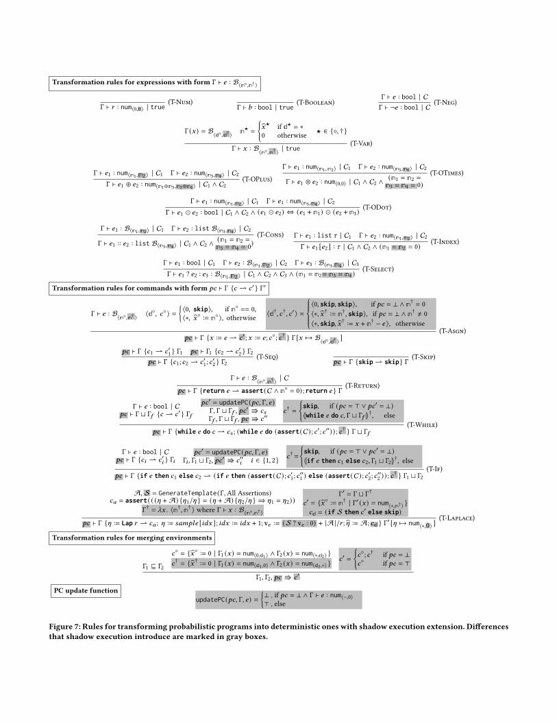
Transformation rules for expressions with form Γ ⊢ 𝑒 : B⟨n◦,n†⟩

Γ ⊢ 𝑟 : num⟨0,0⟩ | true(T-Num)

Γ ⊢ 𝑏 : bool | true (T-Boolean)Γ ⊢ 𝑒 : bool | CΓ ⊢ ¬𝑒 : bool | C (T-Neg)

Γ (𝑥) = B⟨d◦,d† ⟩ n★ =

{��★ if d★ = ∗

0 otherwise ★ ∈ {◦, †}

Γ ⊢ 𝑥 : B⟨n◦,n† ⟩ | true(T-Var)

Γ ⊢ 𝑒1 : num⟨n1,n2 ⟩ | C1 Γ ⊢ 𝑒2 : num⟨n3,n4 ⟩ | C2Γ ⊢ 𝑒1 ⊕ 𝑒2 : num⟨n1⊕n3,n2⊕n4 ⟩ | C1 ∧ C2

(T-OPlus)

Γ ⊢ 𝑒1 : num⟨n1,n2⟩ | C1 Γ ⊢ 𝑒2 : num⟨n3,n4 ⟩ | C2

Γ ⊢ 𝑒1 ⊗ 𝑒2 : num⟨0,0⟩ | C1 ∧ C2 ∧(n1 = n2 =

n3 = n4 = 0)(T-OTimes)

Γ ⊢ 𝑒1 : num⟨n1,n2 ⟩ | C1 Γ ⊢ 𝑒1 : num⟨n3,n4 ⟩ | C2Γ ⊢ 𝑒1 ⊙ 𝑒2 : bool | C1 ∧ C2 ∧ (𝑒1 ⊙ 𝑒2) ⇔ (𝑒1 + n1) ⊙ (𝑒2 + n3)

(T-ODot)

Γ ⊢ 𝑒1 : B⟨n1,n2 ⟩ | C1 Γ ⊢ 𝑒2 : list B⟨n3,n4 ⟩ | C2

Γ ⊢ 𝑒1 :: 𝑒2 : list B⟨n3,n4 ⟩ | C1 ∧ C2 ∧(n1 = n2 =n3 = n4 = 0)

(T-Cons) Γ ⊢ 𝑒1 : list 𝜏 | C1 Γ ⊢ 𝑒2 : num⟨n1,n2 ⟩ | C2Γ ⊢ 𝑒1 [𝑒2 ] : 𝜏 | C1 ∧ C2 ∧ (n1 = n2 = 0) (T-Index)

Γ ⊢ 𝑒1 : bool | C1 Γ ⊢ 𝑒2 : B⟨n1,n2 ⟩ | C2 Γ ⊢ 𝑒3 : B⟨n3,n4 ⟩ | C3Γ ⊢ 𝑒1 ? 𝑒2 : 𝑒3 : B⟨n1,n2 ⟩ | C1 ∧ C2 ∧ C3 ∧ (n1 = n2= n3 = n4 )

(T-Select)

Transformation rules for commands with form 𝑝𝑐 ⊢ Γ {𝑐 ⇀ 𝑐′ } Γ′

Γ ⊢ 𝑒 : B⟨n◦,n† ⟩ ⟨d◦, 𝑐◦ ⟩ =

{⟨0, skip⟩, if n◦ == 0,⟨∗, ��◦ := n◦ ⟩, otherwise ⟨d†, 𝑐†, 𝑐′⟩ =

⟨0, skip, skip⟩, if 𝑝𝑐 = ⊥ ∧ n† = 0⟨∗, ��† := n†, skip⟩, if 𝑝𝑐 = ⊥ ∧ n† ≠ 0⟨∗, skip, ��† := 𝑥 + n† − 𝑒 ⟩, otherwise

𝑝𝑐 ⊢ Γ {𝑥 := 𝑒 ⇀ 𝑐′ ;𝑥 := 𝑒 ;𝑐◦; 𝑐† } Γ [𝑥 ↦→ B⟨d◦,d† ⟩ ](T-Asgn)

𝑝𝑐 ⊢ Γ {𝑐1 ⇀ 𝑐′1 } Γ1 𝑝𝑐 ⊢ Γ1 {𝑐2 ⇀ 𝑐′2 } Γ2𝑝𝑐 ⊢ Γ {𝑐1;𝑐2 ⇀ 𝑐′1;𝑐

′2 } Γ2

(T-Seq)𝑝𝑐 ⊢ Γ {skip ⇀ skip} Γ (T-Skip)

Γ ⊢ 𝑒 : B⟨n◦,n† ⟩ | C𝑝𝑐 ⊢ Γ {return 𝑒 ⇀ assert(C ∧ n◦ = 0) ; return 𝑒 } Γ (T-Return)

Γ ⊢ 𝑒 : bool | C𝑝𝑐 ⊢ Γ ⊔ Γ𝑓 {𝑐 ⇀ 𝑐′ } Γ𝑓

𝑝𝑐′ = updatePC(𝑝𝑐, Γ, 𝑒)Γ, Γ ⊔ Γ𝑓 , 𝑝𝑐

′ ⇛ 𝑐𝑠Γ𝑓 , Γ ⊔ Γ𝑓 , 𝑝𝑐 ⇛ 𝑐′′

𝑐† =

{skip, if (𝑝𝑐 = ⊤ ∨ 𝑝𝑐′ = ⊥)Lwhile 𝑒 do 𝑐, Γ ⊔ Γ𝑓 M†, else

𝑝𝑐 ⊢ Γ {while 𝑒 do 𝑐 ⇀ 𝑐𝑠 ; (while 𝑒 do (assert(C) ;𝑐′;𝑐′′)) ; 𝑐† } Γ ⊔ Γ𝑓(T-While)

Γ ⊢ 𝑒 : bool | C𝑝𝑐 ⊢ Γ {𝑐𝑖 ⇀ 𝑐′𝑖 } Γ𝑖

𝑝𝑐′ = updatePC(𝑝𝑐, Γ, 𝑒)Γ𝑖 , Γ1 ⊔ Γ2, 𝑝𝑐

′ ⇛ 𝑐′′𝑖 𝑖 ∈ {1, 2} 𝑐†=

{skip, if (𝑝𝑐 = ⊤ ∨ 𝑝𝑐′ = ⊥)Lif 𝑒 then 𝑐1 else 𝑐2, Γ1 ⊔ Γ2M†, else

𝑝𝑐 ⊢ Γ {if 𝑒 then 𝑐1 else 𝑐2 ⇀ (if 𝑒 then (assert(C) ;𝑐′1;𝑐′′1 ) else (assert(C) ;𝑐′2;𝑐′′2 )) ; 𝑐† } Γ1 ⊔ Γ2(T-If)

A, S = GenerateTemplate(Γ,All Assertions)𝑐𝑎 = assert( ( ([ + A) {[1/[ } = ([ + A) {[2/[ } ⇒ [1 = [2))

Γ† = _𝑥. ⟨n†,n† ⟩ where Γ ⊢ 𝑥 : B⟨n◦,n†⟩

Γ′ = Γ ⊔ Γ†

𝑐′ = {��◦ := n† | Γ′ (𝑥) = num⟨∗,n†⟩ }𝑐d = (if S then 𝑐′ else skip)

𝑝𝑐 ⊢ Γ {[ := Lap 𝑟 ⇀ 𝑐𝑎 ; [ := 𝑠𝑎𝑚𝑝𝑙𝑒 [𝑖𝑑𝑥 ]; 𝑖𝑑𝑥 := 𝑖𝑑𝑥 + 1; v𝜖 := (S ? v𝜖 : 0) + |A |/𝑟 ; [ := A; 𝑐d } Γ′ [[ ↦→ num⟨∗,0⟩ ](T-Laplace)

Transformation rules for merging environments

Γ1 ⊑ Γ2

𝑐◦ = {��◦ := 0 | Γ1 (𝑥) = num⟨0,d1⟩ ∧ Γ2 (𝑥) = num⟨∗,d2⟩ }𝑐† = {��† := 0 | Γ1 (𝑥) = num⟨d1,0⟩ ∧ Γ2 (𝑥) = num⟨d2,∗⟩ }

𝑐′ =

{𝑐◦;𝑐† if 𝑝𝑐 = ⊥𝑐◦ if 𝑝𝑐 = ⊤

Γ1, Γ2, 𝑝𝑐 ⇛ 𝑐′

PC update functionupdatePC(𝑝𝑐, Γ, 𝑒) =

{⊥ , if 𝑝𝑐 = ⊥ ∧ Γ ⊢ 𝑒 : num⟨−,0⟩⊤ , else

Figure 7: Rules for transforming probabilistic programs into deterministic ones with shadow execution extension. Differencesthat shadow execution introduce are marked in gray boxes.

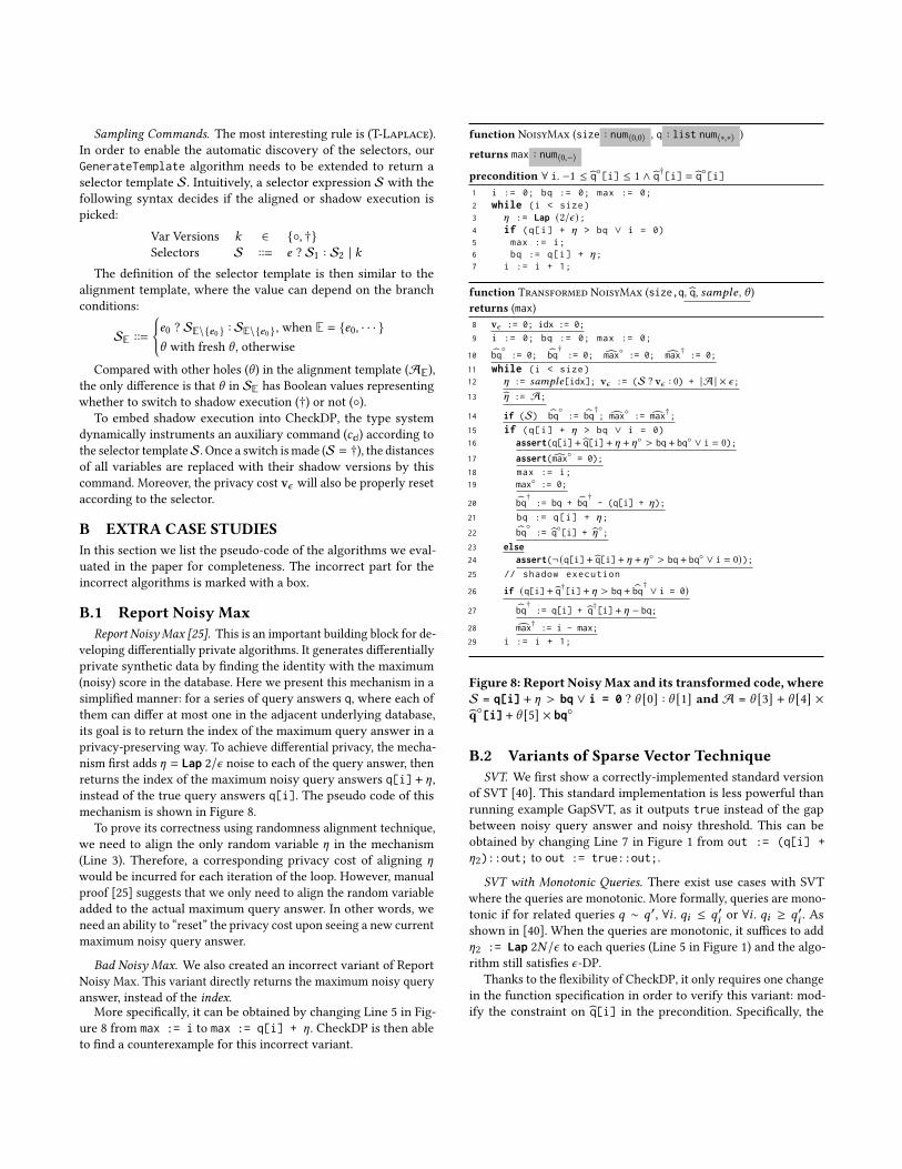
Sampling Commands. The most interesting rule is (T-Laplace).In order to enable the automatic discovery of the selectors, ourGenerateTemplate algorithm needs to be extended to return aselector template S. Intuitively, a selector expression S with thefollowing syntax decides if the aligned or shadow execution ispicked:

Var Versions 𝑘 ∈ {◦, †}Selectors S ::= 𝑒 ? S1 : S2 | 𝑘

The definition of the selector template is then similar to thealignment template, where the value can depend on the branchconditions:

SE ::=

{𝑒0 ? SE\{𝑒0 } : SE\{𝑒0 } , when E = {𝑒0, · · · }\ with fresh \ , otherwise

Compared with other holes (\ ) in the alignment template (AE),the only difference is that \ in SE has Boolean values representingwhether to switch to shadow execution (†) or not (◦).

To embed shadow execution into CheckDP, the type systemdynamically instruments an auxiliary command (𝑐d) according tothe selector templateS. Once a switch is made (S = †), the distancesof all variables are replaced with their shadow versions by thiscommand. Moreover, the privacy cost v𝜖 will also be properly resetaccording to the selector.

B EXTRA CASE STUDIESIn this section we list the pseudo-code of the algorithms we eval-uated in the paper for completeness. The incorrect part for theincorrect algorithms is marked with a box.

B.1 Report Noisy MaxReport Noisy Max [25]. This is an important building block for de-

veloping differentially private algorithms. It generates differentiallyprivate synthetic data by finding the identity with the maximum(noisy) score in the database. Here we present this mechanism in asimplified manner: for a series of query answers q, where each ofthem can differ at most one in the adjacent underlying database,its goal is to return the index of the maximum query answer in aprivacy-preserving way. To achieve differential privacy, the mecha-nism first adds [ = Lap 2/𝜖 noise to each of the query answer, thenreturns the index of the maximum noisy query answers q[i] + [,instead of the true query answers q[i]. The pseudo code of thismechanism is shown in Figure 8.

To prove its correctness using randomness alignment technique,we need to align the only random variable [ in the mechanism(Line 3). Therefore, a corresponding privacy cost of aligning [

would be incurred for each iteration of the loop. However, manualproof [25] suggests that we only need to align the random variableadded to the actual maximum query answer. In other words, weneed an ability to “reset” the privacy cost upon seeing a new currentmaximum noisy query answer.

Bad Noisy Max. We also created an incorrect variant of ReportNoisy Max. This variant directly returns the maximum noisy queryanswer, instead of the index.

More specifically, it can be obtained by changing Line 5 in Fig-ure 8 from max := i to max := q[i] + [. CheckDP is then ableto find a counterexample for this incorrect variant.

function NoisyMax (size : num⟨0,0⟩ , q : list num⟨∗,∗⟩ )

returns max : num⟨0,−⟩

precondition ∀ i. −1 ≤ q◦[i] ≤ 1 ∧ q†[i] = q◦[i]

1 i := 0; bq := 0; max := 0;2 while (i < size)3 [ := Lap (2/𝜖);4 if (q[i] + [ > bq ∨ i = 0)5 max := i;6 bq := q[i] + [;7 i := i + 1;

function Transformed NoisyMax (size,q, q, 𝑠𝑎𝑚𝑝𝑙𝑒 , \ )returns (max)8 v𝜖 := 0; idx := 0;

9 i := 0; bq := 0; max := 0;

10 bq◦:= 0; bq

†:= 0; max◦ := 0; max† := 0;

11 while (i < size)12 [ := 𝑠𝑎𝑚𝑝𝑙𝑒[idx]; v𝜖 := (S ? v𝜖 : 0) + |A | × 𝜖;13 [ := A;

14 if (S) bq◦:= bq

†; max◦ := max†;

15 if (q[i] + [ > bq ∨ i = 0)16 assert(q[i] + q[i] + [ + [◦ > bq + bq◦ ∨ i = 0);17 assert(max◦ = 0);

18 max := i;19 max◦ := 0;

20 bq†:= bq + bq

†- (q[i] + [);

21 bq := q[i] + [;

22 bq◦:= q◦[i] + [

◦;

23 else24 assert(¬(q[i] + q[i] + [ + [◦ > bq + bq◦ ∨ i = 0));25 // shadow execution

26 if (q[i] + q†[i] + [ > bq + bq† ∨ i = 0)

27 bq†:= q[i] + q†[i] + [ − bq;

28 max† := i - max;

29 i := i + 1;

Figure 8: Report NoisyMax and its transformed code, whereS = q[i] + [ > bq ∨ i = 0 ? \ [0] : \ [1] and A = \ [3] + \ [4] ×q◦[i] + \ [5] × bq◦

B.2 Variants of Sparse Vector TechniqueSVT. We first show a correctly-implemented standard version

of SVT [40]. This standard implementation is less powerful thanrunning example GapSVT, as it outputs true instead of the gapbetween noisy query answer and noisy threshold. This can beobtained by changing Line 7 in Figure 1 from out := (q[i] +[2)::out; to out := true::out;.

SVT with Monotonic Queries. There exist use cases with SVTwhere the queries are monotonic. More formally, queries are mono-tonic if for related queries 𝑞 ∼ 𝑞′, ∀𝑖 . 𝑞𝑖 ≤ 𝑞′

𝑖or ∀𝑖 . 𝑞𝑖 ≥ 𝑞′

𝑖. As

shown in [40]. When the queries are monotonic, it suffices to add[2 := Lap 2𝑁 /𝜖 to each queries (Line 5 in Figure 1) and the algo-rithm still satisfies 𝜖-DP.

Thanks to the flexibility of CheckDP, it only requires one changein the function specification in order to verify this variant: mod-ify the constraint on q[i] in the precondition. Specifically, the

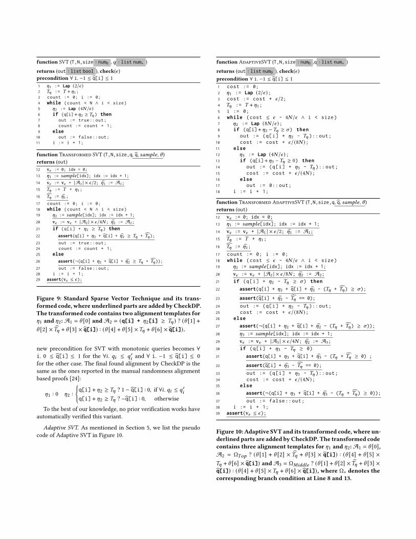
function SVT (T,N,size : num0 , 𝑞 : list num∗ )

returns (out : list bool ), check(𝜖)precondition ∀ i. −1 ≤ q[i] ≤ 11 [1 := Lap (2/𝜖)2 𝑇[ := 𝑇 + [1;3 count := 0; i := 0;4 while (count < N ∧ i < size)5 [2 := Lap (4𝑁 /𝜖)6 if (q[i] + [2 ≥ 𝑇[ ) then7 out := true::out;8 count := count + 1;9 else

10 out := false::out;11 i := i + 1;

function Transformed SVT (T,N,size,q, q, 𝑠𝑎𝑚𝑝𝑙𝑒 , \ )returns (out)12 v𝜖 := 0; idx = 0;

13 [1 := 𝑠𝑎𝑚𝑝𝑙𝑒[idx]; idx := idx + 1;

14 v𝜖 := v𝜖 + |A1 | × 𝜖/2; [1 := A1;

15 𝑇[ := 𝑇 + [1;

16 𝑇[ := [1;

17 count := 0; i := 0;18 while (count < N ∧ i < size)19 [2 := 𝑠𝑎𝑚𝑝𝑙𝑒[idx]; idx := idx + 1;

20 v𝜖 := v𝜖 + |A2 | × 𝜖/4𝑁 ; [2 := A2;

21 if (q[i] + [2 ≥ 𝑇[ ) then22 assert(q[i] + [2 + q[i] + [2 ≥ 𝑇[ + 𝑇[);

23 out := true::out;24 count := count + 1;25 else26 assert(¬(q[i] + [2 + q[i] + [2 ≥ 𝑇[ + 𝑇[));

27 out := false::out;28 i := i + 1;29 assert(v𝜖 ≤ 𝜖);

Figure 9: Standard Sparse Vector Technique and its trans-formed code, where underlined parts are added by CheckDP.The transformed code contains two alignment templates for[1 and [2: A1 = \ [0] and A2 = (q[i] + [2[i] ≥ 𝑇[ ) ? (\ [1] +\ [2] ×𝑇[ + \ [3] × q[i]) : (\ [4] + \ [5] ×𝑇[ + \ [6] × q[i]).

new precondition for SVT with monotonic queries becomes ∀i. 0 ≤ q[i] ≤ 1 for the ∀𝑖 . 𝑞𝑖 ≤ 𝑞′

𝑖and ∀ i. −1 ≤ q[i] ≤ 0

for the other case. The final found alignment by CheckDP is thesame as the ones reported in the manual randomness alignmentbased proofs [24]:

[1 : 0 [2 :

{q[i] + [2 ≥ 𝑇[ ? 1 − q[i] : 0, if ∀𝑖 . 𝑞𝑖 ≤ 𝑞′

𝑖

q[i] + [2 ≥ 𝑇[ ? −q[i] : 0, otherwise

To the best of our knowledge, no prior verification works haveautomatically verified this variant.

Adaptive SVT. As mentioned in Section 5, we list the pseudocode of Adaptive SVT in Figure 10.

function AdaptiveSVT (T,N,size : num0 ,q : list num∗ )

returns (out : list num0 ), check(𝜖)precondition ∀ i. −1 ≤ q[i] ≤ 11 cost := 0;2 [1 := Lap (2/𝜖);3 cost := cost + 𝜖/2;4 𝑇[ := 𝑇 + [1;5 i := 0;6 while (cost ≤ 𝜖 - 4𝑁 /𝜖 ∧ i < size)7 [2 := Lap (8𝑁 /𝜖);8 if (q[i] + [2 −𝑇[ ≥ 𝜎) then9 out := (q[i] + [2 - 𝑇[ )::out;

10 cost := cost + 𝜖/(8𝑁 );11 else12 [3 := Lap (4𝑁 /𝜖);13 if (q[i] + [3 −𝑇[ ≥ 0) then14 out := (q[i] + [3 - 𝑇[ )::out;15 cost := cost + 𝜖/(4𝑁 );16 else17 out := 0::out;18 i := i + 1;

function Transformed AdaptiveSVT (T,N,size,q, q, 𝑠𝑎𝑚𝑝𝑙𝑒 , \ )returns (out)12 v𝜖 := 0; idx = 0;

13 [1 := 𝑠𝑎𝑚𝑝𝑙𝑒[idx]; idx := idx + 1;

14 v𝜖 := v𝜖 + |A1 | × 𝜖/2; [1 := A1;

15 𝑇[ := 𝑇 + [1;

16 𝑇[ := [1;

17 count := 0; i := 0;18 while (cost ≤ 𝜖 - 4𝑁 /𝜖 ∧ i < size)19 [2 := 𝑠𝑎𝑚𝑝𝑙𝑒[idx]; idx := idx + 1;

20 v𝜖 := v𝜖 + |A2 | × 𝜖/8𝑁; [2 := A2;

21 if (q[i] + [2 - 𝑇[ ≥ 𝜎) then

22 assert(q[i] + [2 + q[i] + [2 - (𝑇[ + 𝑇[) ≥ 𝜎);

23 assert(q[i] + [2 - 𝑇[ == 0);

24 out := (q[i] + [2 - 𝑇[ )::out;25 cost := cost + 𝜖/(8𝑁 );26 else

27 assert(¬(q[i] + [2 + q[i] + [2 - (𝑇[ + 𝑇[) ≥ 𝜎));

28 [3 := 𝑠𝑎𝑚𝑝𝑙𝑒[idx]; idx := idx + 1;

29 v𝜖 := v𝜖 + |A3 | × 𝜖/4𝑁 ; [2 := A3;

30 if (q[i] + [3 - 𝑇[ ≥ 0)

31 assert(q[i] + [3 + q[i] + [3 - (𝑇[ + 𝑇[ ≥ 0) ;

32 assert(q[i] + [3 - 𝑇[ == 0);

33 out := (q[i] + [3 - 𝑇[ )::out;34 cost := cost + 𝜖/(4𝑁 );35 else

36 assert(¬(q[i] + [3 + q[i] + [3 - (𝑇[ + 𝑇[) ≥ 0));

37 out := false::out;38 i := i + 1;39 assert(v𝜖 ≤ 𝜖);

Figure 10: Adaptive SVT and its transformed code, where un-derlined parts are added by CheckDP. The transformed codecontains three alignment templates for [1 and [2:A1 = \ [0],A2 = Ω𝑇𝑜𝑝 ? (\ [1] + \ [2] × 𝑇[ + \ [3] × q[i]) : (\ [4] + \ [5] ×𝑇[ + \ [6] × q[i]) and A3 = Ω𝑀𝑖𝑑𝑑𝑙𝑒 ? (\ [1] + \ [2] ×𝑇[ + \ [3] ×q[i]) : (\ [4] + \ [5] ×𝑇[ + \ [6] × q[i]), where Ω∗ denotes thecorresponding branch condition at Line 8 and 13.

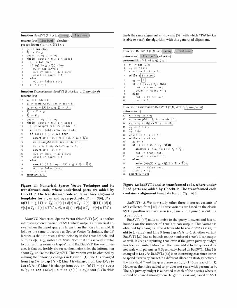
function NumSVT (T,N,size : num0 , 𝑞 : list num∗ )

returns (out : list bool ), check(𝜖)precondition ∀ i. −1 ≤ q[i] ≤ 11 [1 := Lap (3/𝜖)2 𝑇[ := 𝑇 + [1;3 count := 0; i := 0;4 while (count < N ∧ i < size)5 [2 := Lap (6𝑁 /𝜖)6 if (q[i] + [2 ≥ 𝑇[ ) then7 [3 := Lap (3𝑁 /𝜖);8 out := (q[i] + [3)::out;9 count := count + 1;

10 else11 out := false::out;12 i := i + 1;

function Transformed NumSVT (T,N,size,q, q, 𝑠𝑎𝑚𝑝𝑙𝑒 , \ )returns (out)12 v𝜖 := 0; idx = 0;

13 [1 := 𝑠𝑎𝑚𝑝𝑙𝑒[idx]; idx := idx + 1;

14 v𝜖 := v𝜖 + |A1 | × 𝜖/3; [1 := A1;

15 𝑇[ := 𝑇 + [1;

16 𝑇[ := [1;

17 count := 0; i := 0;18 while (count < N ∧ i < size)19 [2 := 𝑠𝑎𝑚𝑝𝑙𝑒[idx]; idx := idx + 1;

20 v𝜖 := v𝜖 + |A2 | × 𝜖/6𝑁 ; [2 := A2;

21 if (q[i] + [2 ≥ 𝑇[ ) then22 assert(q[i] + [2 + q[i] + [2 ≥ 𝑇[ + 𝑇[);

23 [3 := 𝑠𝑎𝑚𝑝𝑙𝑒[idx]; idx := idx + 1;

24 v𝜖 := v𝜖 + |A3 | × 𝜖/3𝑁 ; [3 := A3;

25 assert(q[i] + [3 = 0);

26 out := (q[i] + [3)::out;27 count := count + 1;28 else29 assert(¬(q[i] + [2 + q[i] + [2 ≥ 𝑇[ + 𝑇[));

30 out := false::out;31 i := i + 1;32 assert(v𝜖 ≤ 𝜖);

Figure 11: Numerical Sparse Vector Technique and itstransformed code, where underlined parts are added byCheckDP. The transformed code contains three alignmenttemplates for [1, [2 and [3 respectively: A1 = \ [0], A2 =

(q[i] + [2[i] ≥ 𝑇[ ) ? (\ [1] + \ [2] ×𝑇[ + \ [3] × q[i]) : (\ [4] +\ [5] ×𝑇[ + \ [6] × q[i]), A3 = \ [7] + \ [8] ×𝑇[ + \ [9] × q[i])

NumSVT. Numerical Sparse Vector (NumSVT) [28] is anotherinteresting correct variant of SVT which outputs a numerical an-swer when the input query is larger than the noisy threshold. Itfollows the same procedure as Sparse Vector Technique, the dif-ference is that it draws a fresh noise [3 in the true branch, andoutputs 𝑞 [𝑖] + [3 instead of true. Note that this is very similarto our running example GapSVT and BadGapSVT, the key differ-ence is that the freshly-drawn random noise hides the informationabout 𝑇[ , unlike the BadGapSVT. This variant can be obtained bymaking the following changes in Figure 1: (1) Line 1 is changedfrom Lap 2/𝜖 to Lap 3/𝜖; (2) Line 5 is changed from Lap 4𝑁 /𝜖 toLap 6𝑁 /𝜖; (3) Line 7 is change from out := (q[i] + [)::out;to “[3 := Lap (3𝑁 /𝜖); out := (q[i] + [3)::out;”. CheckDP

finds the same alignment as shown in [52] with which CPACheckeris able to verify the algorithm with this generated alignment.

function BadSVT1 (T,N,size : num0 , 𝑞 : list num∗ )

returns (out : list bool ), check(𝜖)precondition ∀ i. −1 ≤ q[i] ≤ 11 [1 := Lap (2/𝜖);2 𝑇[ := 𝑇 + [1;3 count := 0; i := 0;

4 while ( i < size )

5 [2 := 0 ;

6 if (q[i] + [2 ≥ 𝑇[ ) then7 out := true::out;8 count := count + 1;9 else

10 out := false::out;11 i := i + 1;

function Transformed BadSVT1 (T,N,size,q, q, 𝑠𝑎𝑚𝑝𝑙𝑒 , \ )returns (out)12 v𝜖 := 0; idx = 0;

13 [1 := 𝑠𝑎𝑚𝑝𝑙𝑒[idx]; idx := idx + 1;

14 v𝜖 := v𝜖 + |A1 | × 𝜖/2; [1 := A1;

15 𝑇[ := 𝑇 + [1;

16 𝑇[ := [1;

17 count := 0; i := 0;18 while (i < size)19 [2 := 0;20 if (q[i] + [2 ≥ 𝑇[ ) then21 assert(q[i] + [2 + q[i] ≥ 𝑇[ + 𝑇[);

22 out := true::out;23 count := count + 1;24 else25 assert(¬(q[i] + [2 + q[i] ≥ 𝑇[ + 𝑇[));

26 out := false::out;27 i := i + 1;28 assert(v𝜖 ≤ 𝜖);

Figure 12: BadSVT1 and its transformed code, where under-lined parts are added by CheckDP. The transformed codecontains a alignment template for [1: A1 = \ [0].

BadSVT1 - 3. We now study other three incorrect variants ofSVT collected from [40]. All three variants are based on the classicSVT algorithm we have seen (i.e., Line 7 in Figure 1 is out :=true::out;).

BadSVT1 [47] adds no noise to the query answers and has nobounds on the number of true’s it can output. This variant isobtained by changing Line 4 from while (count<N∧i<size) towhile (i<size) and Line 5 from Lap 4𝑁 /𝜖 to 0. Another variantBadSVT2 [20] has no bounds on the number of true’s it can outputas well. It keeps outputting true even if the given privacy budgethas been exhausted. Moreover, the noise added to the queries doesnot scale with parameter N. Specifically, based on BadSVT1, Line 5 ischanged to Lap 2/𝜖 . BadSVT3 [38] is an interesting case since it triesto spend its privacy budget in a different allocation strategy betweenthe threshold T and the query answers q[i] (1 : 3 instead of 1 : 1).However, the noise added to [2 does not scale with parameter N.The 3/4 privacy budget is allocated to each of the queries where itshould be shared among them. To get this variant, based on SVT

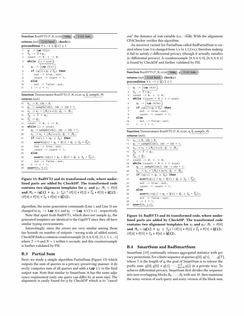
function BadSVT2 (T,N,size : num0 , 𝑞 : list num∗ )

returns (out : list bool ), check(𝜖)precondition ∀ i. −1 ≤ q[i] ≤ 11 [1 := Lap (2/𝜖);2 𝑇[ := 𝑇 + [1;3 count := 0; i := 0;

4 while ( i < size )

5 [2 := Lap (2/𝜖) ;

6 if (q[i] + [2 ≥ 𝑇[ ) then7 out := true::out;8 count := count + 1;9 else

10 out := false::out;11 i := i + 1;

function Transformed BadSVT2 (T,N,size,q, q, 𝑠𝑎𝑚𝑝𝑙𝑒 , \ )returns (out)12 v𝜖 := 0; idx = 0;

13 [1 := 𝑠𝑎𝑚𝑝𝑙𝑒[idx]; idx := idx + 1;

14 v𝜖 := v𝜖 + |A1 | × 𝜖/2; [1 := A1;

15 𝑇[ := 𝑇 + [1;

16 𝑇[ := [1;

17 count := 0; i := 0;18 while (i < size)19 [2 := 𝑠𝑎𝑚𝑝𝑙𝑒[idx]; idx := idx + 1;

20 v𝜖 := v𝜖 + |A2 | × 𝜖/2; [2 := A2;

21 if (q[i] + [2 ≥ 𝑇[ ) then22 assert(q[i] + [2 + q[i] + [2 ≥ 𝑇[ + 𝑇[);

23 out := true::out;24 count := count + 1;25 else26 assert(¬(q[i] + [2 + q[i] + [2 ≥ 𝑇[ + 𝑇[));

27 out := false::out;28 i := i + 1;29 assert(v𝜖 ≤ 𝜖);

Figure 13: BadSVT2 and its transformed code, where under-lined parts are added by CheckDP. The transformed codecontains two alignment templates for [1 and [2: A1 = \ [0]and A2 = (q[i] + [2 ≥ 𝑇[ ) ? (\ [1] + \ [2] ×𝑇[ + \ [3] × q[i]) :(\ [4] + \ [5] ×𝑇[ + \ [6] × q[i]).

algorithm, the noise generation commands (Line 1 and Line 5) arechanged to [1 := Lap 4/𝜖 and [2 := Lap 4/(3 × 𝜖) , respectively.

Note that apart from BadSVT1, which does not sample [2, thegenerated templates are identical to the GapSVT since they all havesimilar typing environments.

Interestingly, since the errors are very similar among them(no bounds on number of outputs / wrong scale of added noise),CheckDP finds a common counterexample [0, 0, 0, 0, 0], [1, 1, 1, 1,−1]where 𝑇 = 0 and 𝑁 = 1 within 6 seconds, and this counterexampleis further validated by PSI.

B.3 Partial SumNext, we study a simple algorithm PartialSum (Figure 15) whichoutputs the sum of queries in a privacy-preserving manner: it di-rectly computes sum of all queries and adds a Lap 1/𝜖 to the finaloutput sum. Note that similar to SmartSum, it has the same adja-cency requirement (only one query can differ by at most one). Thealignment is easily found for [ by CheckDP which is to “cancel

out” the distance of sum variable (i.e., -sum). With the alignmentCPAChecker verifies this algorithm.

An incorrect variant for PartialSum called BadPartialSum is cre-ated where Line 5 is changed from 1/𝜖 to 1/(2×𝜖), therefore makingit fail to satisfy 𝜖-differential privacy (though it actually satisfies2𝜖-differential privacy). A counterexample [0, 0, 0, 0, 0], [0, 0, 0, 0, 1]is found by CheckDP and further validated by PSI.

function BadSVT3 (T,N,size : num0 , 𝑞 : list num∗ )

returns (out : list bool ), check(𝜖)precondition ∀ i. −1 ≤ q[i] ≤ 1

1 [1 := Lap (4/𝜖) ;

2 𝑇[ := 𝑇 + [1;3 count := 0; i := 0;4 while (count < N ∧ i < size)

5 [2 := Lap (4/3𝜖) ;

6 if (q[i] + [2 ≥ 𝑇[ ) then7 out := true::out;8 count := count + 1;9 else

10 out := false::out;11 i := i + 1;

function Transformed BadSVT3 (T,N,size,q, q, 𝑠𝑎𝑚𝑝𝑙𝑒 , \ )returns (out)12 v𝜖 := 0; idx = 0;

13 [1 := 𝑠𝑎𝑚𝑝𝑙𝑒[idx]; idx := idx + 1;

14 v𝜖 := v𝜖 + |A1 | × 𝜖/4; [1 := A1;

15 𝑇[ := 𝑇 + [1;

16 𝑇[ := [1;

17 count := 0; i := 0;18 while (count < N ∧ i < size)19 [2 := 𝑠𝑎𝑚𝑝𝑙𝑒[idx]; idx := idx + 1;

20 v𝜖 := v𝜖 + |A2 | × 3𝜖/4; [2 := A2;

21 if (q[i] + [2 ≥ 𝑇[ ) then22 assert(q[i] + [2 + q[i] + [2 ≥ 𝑇[ + 𝑇[);

23 out := true::out;24 count := count + 1;25 else26 assert(¬(q[i] + [2 + q[i] + [2 ≥ 𝑇[ + 𝑇[));

27 out := false::out;28 i := i + 1;29 assert(v𝜖 ≤ 𝜖);

Figure 14: BadSVT3 and its transformed code, where under-lined parts are added by CheckDP. The transformed codecontains two alignment templates for [1 and [2: A1 = \ [0]and A2 = (q[i] + [2 ≥ 𝑇[ ) ? (\ [1] + \ [2] ×𝑇[ + \ [3] × q[i]) :(\ [4] + \ [5] ×𝑇[ + \ [6] × q[i]).

B.4 SmartSum and BadSmartSumSmartSum [19] continually releases aggregated statistics with pri-vacy protections. For a finite sequence of queries𝑞 [0], 𝑞[1], · · · , 𝑞[𝑇 ],where 𝑇 is the length of 𝑞, the goal of SmartSum is to release theprefix sum: 𝑞 [0], 𝑞[0] + 𝑞 [1], · · · ,∑𝑇

𝑖=0 𝑞 [𝑖] in a private way. Toachieve differential privacy, SmartSum first divides the sequenceinto non-overlapping blocks 𝐵0, · · · , 𝐵𝑙 with size𝑀 , then maintainsthe noisy version of each query and noisy version of the block sum,

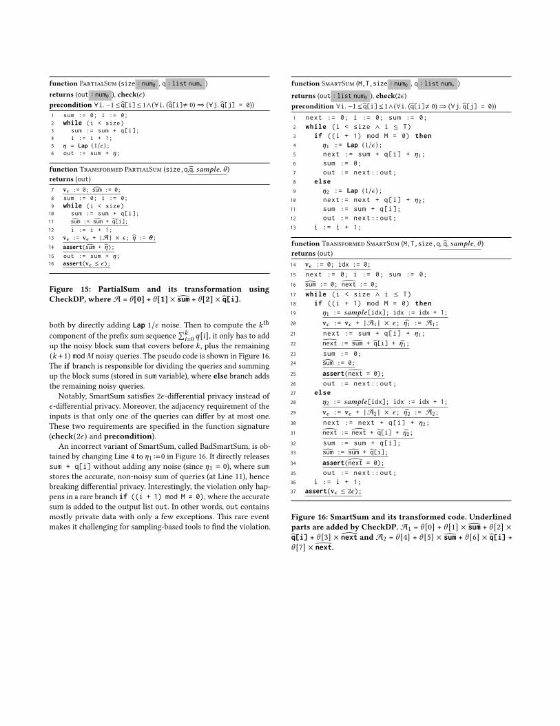
function PartialSum (size : num0 , q : list num∗ )returns (out : num0 ), check(𝜖)precondition ∀i. −1 ≤ q[i]≤ 1∧(∀i. (q[i]≠ 0)⇒ (∀j. q[j] = 0))1 sum := 0; i := 0;2 while (i < size)3 sum := sum + q[i];4 i := i + 1;5 [ = Lap (1/𝜖);6 out := sum + [;

function Transformed PartialSum (size,q,q, 𝑠𝑎𝑚𝑝𝑙𝑒 , \ )returns (out)7 v𝜖 := 0; sum := 0;

8 sum := 0; i := 0;9 while (i < size)

10 sum := sum + q[i];11 sum := sum + q[i];

12 i := i + 1;13 v𝜖 := v𝜖 + |A| × 𝜖; [ := 𝜽;

14 assert(sum + [);

15 out := sum + [;16 assert(v𝜖 ≤ 𝜖);

Figure 15: PartialSum and its transformation usingCheckDP, where A = \[0] + \[1] × sum + \[2] × q[i].

both by directly adding Lap 1/𝜖 noise. Then to compute the 𝑘th

component of the prefix sum sequence∑𝑘𝑖=0 𝑞 [𝑖], it only has to add

up the noisy block sum that covers before 𝑘 , plus the remaining(𝑘 + 1) mod𝑀 noisy queries. The pseudo code is shown in Figure 16.The if branch is responsible for dividing the queries and summingup the block sums (stored in sum variable), where else branch addsthe remaining noisy queries.

Notably, SmartSum satisfies 2𝜖-differential privacy instead of𝜖-differential privacy. Moreover, the adjacency requirement of theinputs is that only one of the queries can differ by at most one.These two requirements are specified in the function signature(check(2𝜖) and precondition).

An incorrect variant of SmartSum, called BadSmartSum, is ob-tained by changing Line 4 to [1 :=0 in Figure 16. It directly releasessum + q[i] without adding any noise (since [1 = 0), where sumstores the accurate, non-noisy sum of queries (at Line 11), hencebreaking differential privacy. Interestingly, the violation only hap-pens in a rare branch if ((i + 1) mod M = 0), where the accuratesum is added to the output list out. In other words, out containsmostly private data with only a few exceptions. This rare eventmakes it challenging for sampling-based tools to find the violation.

function SmartSum (M,T,size : num0 , q : list num∗ )

returns (out : list num0 ), check(2𝜖)precondition ∀i. −1 ≤ q[i]≤ 1∧(∀i. (q[i]≠ 0)⇒ (∀j. q[j] = 0))1 next := 0; i := 0; sum := 0;2 while (i < size ∧ i ≤ T)3 if ((i + 1) mod M = 0) then4 [1 := Lap (1/𝜖);5 next := sum + q[i] + [1;6 sum := 0;7 out := next::out;8 else9 [2 := Lap (1/𝜖);

10 next:= next + q[i] + [2;11 sum := sum + q[i];12 out := next::out;13 i := i + 1;

function Transformed SmartSum (M,T,size,q, q, 𝑠𝑎𝑚𝑝𝑙𝑒 , \ )returns (out)14 v𝜖 := 0; idx := 0;

15 next := 0; i := 0; sum := 0;

16 sum := 0; �next := 0;

17 while (i < size ∧ i ≤ T)18 if ((i + 1) mod M = 0) then19 [1 := 𝑠𝑎𝑚𝑝𝑙𝑒[idx]; idx := idx + 1;

20 v𝜖 := v𝜖 + |A1| × 𝜖; [1 := A1;

21 next := sum + q[i] + [1;

22 �next := sum + q[i] + [1;

23 sum := 0;24 sum := 0;

25 assert(�next = 0);

26 out := next::out;27 else28 [2 := 𝑠𝑎𝑚𝑝𝑙𝑒[idx]; idx := idx + 1;

29 v𝜖 := v𝜖 + |A2| × 𝜖; [2 := A2;

30 next := next + q[i] + [2;

31 �next := �next + q[i] + [2;

32 sum := sum + q[i];33 sum := sum + q[i];

34 assert(�next = 0);

35 out := next::out;36 i := i + 1;37 assert(v𝜖 ≤ 2𝜖);

Figure 16: SmartSum and its transformed code. Underlinedparts are added by CheckDP. A1 = \ [0] + \ [1] × sum + \ [2] ×q[i] + \ [3] ×�next and A2 = \ [4] + \ [5] × sum + \ [6] × q[i] +\ [7] ×�next.