9-1CHBE320 Process Dynamics and Control Korea University

CHBE320 LECTURE IXFREQUENCY RESPONSES

Professor Dae Ryook Yang

Fall 2019Dept. of Chemical and Biological Engineering

Korea University

9-2CHBE320 Process Dynamics and Control Korea University

Road Map of the Lecture IX

• Frequency Response– Definition– Benefits of frequency analysis– How to get frequency response– Bode Plot– Nyquist Diagram

9-3CHBE320 Process Dynamics and Control Korea University

DEFINITION OF FREQUENCY RESPONSE

• For linear system– “The ultimate output response of a process for a sinusoidal

input at a frequency will show amplitude change and phase shift at the same frequency depending on the process characteristics.”

– Amplitude ratio (AR): attenuation of amplitude,– Phase angle ( 𝜙 ): phase shift compared to input– These two quantities are the function of frequency.

ProcessInput Output

𝐴 sin 𝜔 𝑡 𝐴 sin 𝜔𝑡 𝜙

After all transient effects are decayed out.

t

𝜑

𝑢 𝑡

𝑦 𝑡

-A

A𝐴

𝐴

𝐴/𝐴

9-4CHBE320 Process Dynamics and Control Korea University

BENEFITS OF FREQUENCY RESPONSE

• Frequency responses are the informative representations of dynamic systems– Audio Speaker

– Equalizer

– Structure

Elec. Signal Sound wave

Raw signal

Processedsignal

Expensive speaker

Cheap speaker

Old Tacoma bridge New Tacoma bridge

Old Tacoma bridge

New Tacoma bridge

Adjustable for each

frequency band

9-5CHBE320 Process Dynamics and Control Korea University

– Low-pass filter

– High-pass filter

– In signal processing field, transfer functions are called “filters”.

9-6CHBE320 Process Dynamics and Control Korea University

• Any linear dynamical system is completely defined by its frequency response.– The AR and phase angle define the system completely.– Bode diagram

• AR in log-log plot• Phase angle in log-linear plot

– Via efficient numerical technique (fast Fourier transform, FFT), the output can be calculated for any type of input.

• Frequency response representation of a system dynamics is very convenient for designing a feedback controller and analyzing a closed-loop system. – Bode stability– Gain margin (GM) and phase margin (PM)

9-7CHBE320 Process Dynamics and Control Korea University

• Critical frequency– As frequency changes, the amplitude ratio (AR) and the phase

angle (PA) change.– The frequency where the PA reaches –180° is called critical

frequency (c).– The component of output at the critical frequency will have the

exactly same phase as the signal goes through the loop due to comparator (-180 °) and phase shift of the process (-180 °).

– For the open-loop gain at the critical frequency, • No change in magnitude• Continuous cycling

– For • Getting bigger in magnitude• Unstable

– For• Getting smaller in magnitude• Stable

𝐾 𝜔 1

R Gc …GP+

-YE

Sign change

Sign change

𝐾 𝜔 1

𝐾 𝜔 1

9-8CHBE320 Process Dynamics and Control Korea University

• Example– If a feed is pumped by a peristaltic pump to a CSTR, will the

fluctuation of the feed flow appear in the output?

– V=50cm3, q=90cm3/min (so is the average of qi)• Process time constant=0.555min.

– The rpm of the peristaltic pump is 60rpm.• Input frequency=180rad/min (3blades)

– The AR=0.01

t

qi

V

cAi, qi

Peristaltic pump cA, q

If the magnitude of fluctuation of qi is 5% of nominal flow rate, the fluctuation in the output concentration will be about 0.05% which is almost unnoticeable.

𝑉𝑑𝑐𝑑𝑡 𝑞 𝑐 𝑞𝑐 𝑞 constant

𝐶 𝑠𝑞 𝑠

𝐶𝑉𝑠 𝑞

𝐶 /𝑞𝑉/𝑞 𝑠 1

𝜔𝜏 100

9-9CHBE320 Process Dynamics and Control Korea University

OBTAINING FREQUENCY RESPONSE

• From the transfer function, replace s with

– For a pole, , the response mode is .– If the modes are not unstable ( ) and enough time elapses,

the survived modes becomes . (ultimate response)

• The frequency response, is complex as a function of frequency.

𝑗𝜔

𝐺 𝑠

𝐺 𝑗𝜔Transfer function Frequency response

𝐺 𝑗𝜔

𝐺 𝑗𝜔 Re 𝐺 𝑗𝜔 𝑗 Im 𝐺 𝑗𝜔

𝐴𝑅 𝐺 𝑗𝜔 Re 𝐺 𝑗𝜔 Im 𝐺 𝑗𝜔

𝜙 ∡𝐺 𝑗𝜔 tan Im 𝐺 𝑗𝜔 / Re 𝐺 𝑗𝜔

𝑠 𝛼 𝑗𝜔 𝑒

𝛼 0

𝑒

Re

Im

𝜑

𝐺 𝑗𝜔

AR

𝜔 ↑

Nyquist diagram

Bode plot

9-10CHBE320 Process Dynamics and Control Korea University

• Getting ultimate response– For a sinusoidal forcing function– Assume G(s) has stable poles bi.

– Without calculating transient response, the frequency response can be obtained directly from .

– Unstable transfer function does not have a frequency response because a sinusoidal input produces an unstable output response.

𝑌 𝑠 𝐺 𝑠𝐴𝜔

𝑠 𝜔

𝑌 𝑠 𝐺 𝑠𝐴𝜔

𝑠 𝜔𝛼

𝑠 𝑏 ⋯𝛼

𝑠 𝑏𝐶𝑠 𝐷𝜔𝑠 𝜔

𝐺 𝑗𝜔 𝐴𝜔 𝐶𝑗𝜔 𝐷𝜔 ⇒ 𝐺 𝑗𝜔𝐷𝐴 𝑗

𝐶𝐴 𝑅 𝑗𝐼

Decayed out at large t

𝐶 𝐼𝐴, 𝐷 𝑅𝐴 ⇒ 𝑦 𝐴 𝐼 cos 𝜔 𝑡 𝑅 sin 𝜔 𝑡 𝐴 sin 𝜔𝑡 𝜙

∴ 𝐴𝑅 𝐴/𝐴 𝑅 𝐼 𝐺 𝑗𝜔 and 𝜙 tan 𝐼/𝑅 ∡𝐺 𝑗𝜔

𝐺 𝑗𝜔

9-11CHBE320 Process Dynamics and Control Korea University

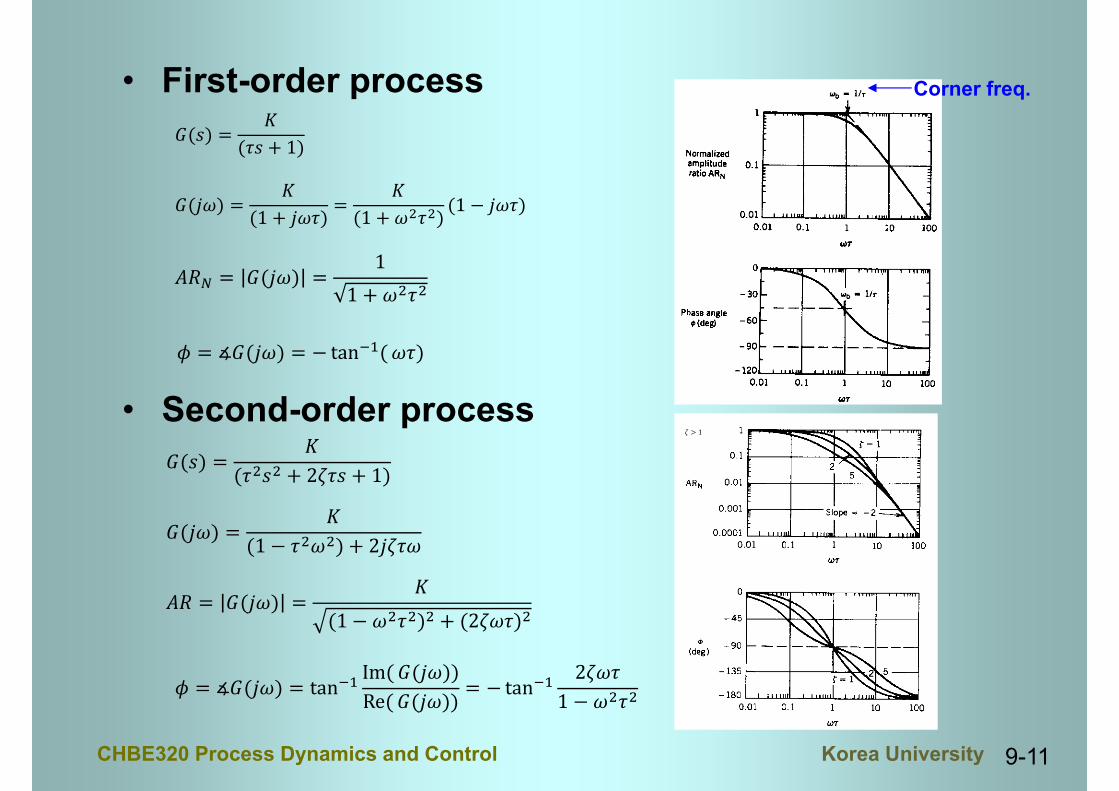
• First-order process

• Second-order process

𝐺 𝑠𝐾

𝜏𝑠 1

𝐺 𝑗𝜔𝐾

1 𝑗𝜔𝜏𝐾

1 𝜔 𝜏 1 𝑗𝜔𝜏

𝐴𝑅 𝐺 𝑗𝜔1

1 𝜔 𝜏

𝜙 ∡𝐺 𝑗𝜔 tan 𝜔𝜏

𝐺 𝑠𝐾

𝜏 𝑠 2𝜁𝜏𝑠 1

𝐺 𝑗𝜔𝐾

1 𝜏 𝜔 2𝑗𝜁𝜏𝜔

𝐴𝑅 𝐺 𝑗𝜔𝐾

1 𝜔 𝜏 2𝜁𝜔𝜏

𝜙 ∡𝐺 𝑗𝜔 tanIm 𝐺 𝑗𝜔Re 𝐺 𝑗𝜔 tan

2𝜁𝜔𝜏1 𝜔 𝜏

𝜁 1

Corner freq.

9-12CHBE320 Process Dynamics and Control Korea University

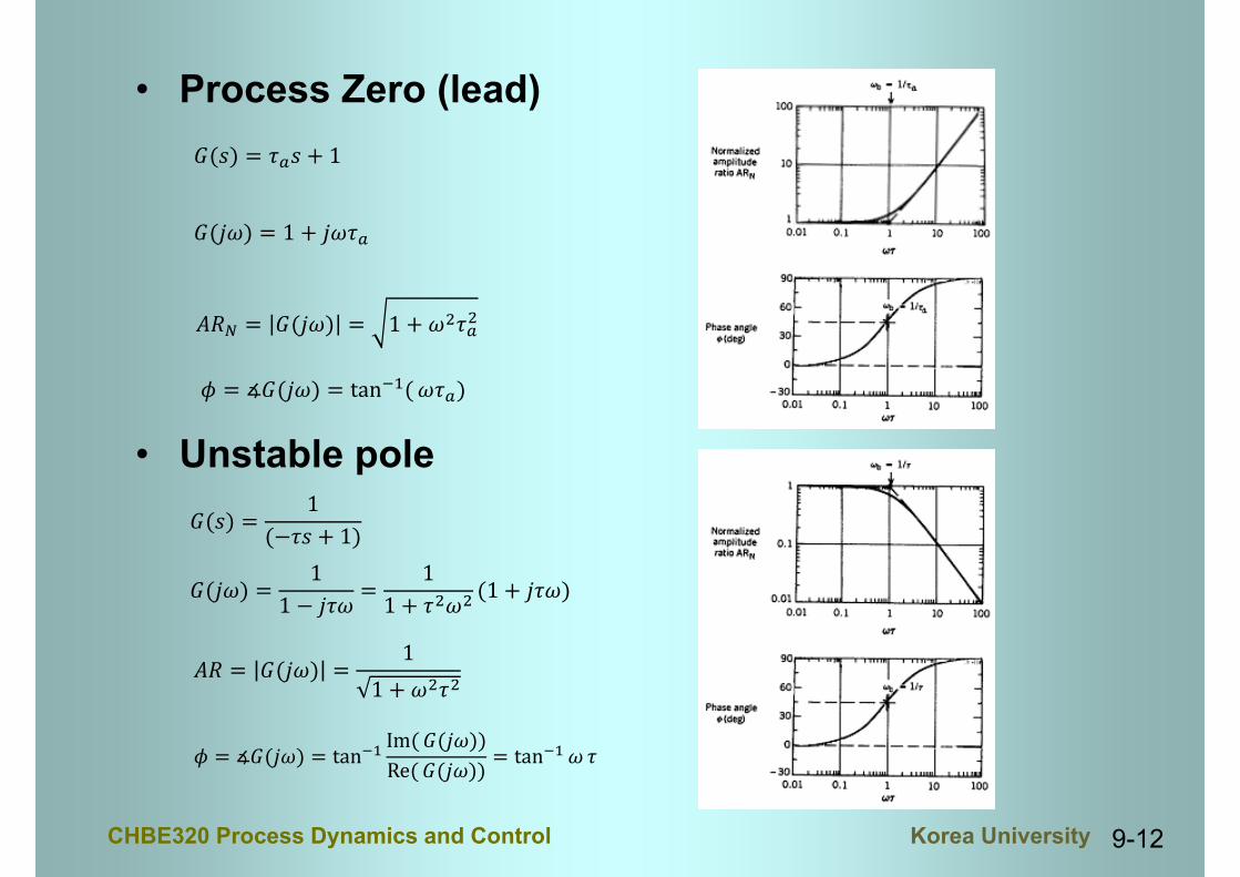
• Process Zero (lead)

• Unstable pole

𝐺 𝑠 𝜏 𝑠 1

𝐺 𝑗𝜔 1 𝑗𝜔𝜏

𝐴𝑅 𝐺 𝑗𝜔 1 𝜔 𝜏

𝜙 ∡𝐺 𝑗𝜔 tan 𝜔𝜏

𝐺 𝑠1

𝜏𝑠 1

𝐺 𝑗𝜔1

1 𝑗𝜏𝜔1

1 𝜏 𝜔 1 𝑗𝜏𝜔

𝐴𝑅 𝐺 𝑗𝜔1

1 𝜔 𝜏

𝜙 ∡𝐺 𝑗𝜔 tanIm 𝐺 𝑗𝜔Re 𝐺 𝑗𝜔 tan 𝜔 𝜏

9-13CHBE320 Process Dynamics and Control Korea University

• Integrating process

• Differentiator

• Pure delay process

𝐺 𝑠1

𝐴𝑠 𝐺 𝑗𝜔1

𝑗𝐴𝜔1

𝐴𝜔 𝑗

𝐴𝑅 𝐺 𝑗𝜔1

𝐴𝜔

𝜙 ∡𝐺 𝑗𝜔 tan1

0 ⋅ 𝜔𝜋2

𝐺 𝑠 𝑒

𝐺 𝑗𝜔 𝑒 cos 𝜃 𝜔 𝑗 sin 𝜃 𝜔

𝐴𝑅 𝐺 𝑗𝜔 1

𝜙 ∡𝐺 𝑗𝜔 tan tan 𝜃 𝜔 𝜃𝜔

𝐺 𝑠 𝐴𝑠 𝐺 𝑗𝜔 𝑗𝐴𝜔

𝐴𝑅 𝐺 𝑗𝜔 𝐴𝜔

𝜙 ∡𝐺 𝑗𝜔 tan1

0 ⋅ 𝜔𝜋2

9-14CHBE320 Process Dynamics and Control Korea University

SKETCHING BODE PLOT

• Bode diagram– AR vs. frequency in log-log plot– PA vs. frequency in semi-log plot– Useful for

• Analysis of the response characteristics• Stability of the closed-loop system only for open-loop stable

systems with phase angle curves exhibit a single critical frequency.

𝐺 𝑠𝐺 𝑠 𝐺 𝑠 𝐺 𝑠 ⋯𝐺 𝑠 𝐺 𝑠 𝐺 𝑠 ⋯ 𝐺 𝑗𝜔

𝐺 𝑗𝜔 𝐺 𝑗𝜔 𝐺 𝑗𝜔 ⋯𝐺 𝑗𝜔 𝐺 𝑗𝜔 𝐺 𝑗𝜔 ⋯

𝐺 𝑗𝜔𝐺 𝑗𝜔 𝐺 𝑗𝜔 𝐺 𝑗𝜔 ⋯𝐺 𝑗𝜔 𝐺 𝑗𝜔 𝐺 𝑗𝜔 ⋯

∡𝐺 𝑗𝜔 ∡𝐺 𝑗𝜔 ∡𝐺 𝑗𝜔 ∡𝐺 𝑗𝜔 ⋯ ∡𝐺 𝑗𝜔 ∡𝐺 𝑗𝜔 ∡𝐺 𝑗𝜔 ⋯

9-15CHBE320 Process Dynamics and Control Korea University

• Amplitude Ratio on log-log plot– Start from steady-state gain at = 0. If GOL includes either

integrator or differentiator it starts at ∞ or 0.– Each first-order lag (lead) adds to the slope –1 (+1) starting at

the corner frequency.– Each integrator (differentiator) adds to the slope –1 (+1)

starting at zero frequency.– A delays does not contribute to the AR plot.

• Phase angle on semi-log plot– Start from 0° or -180° at = 0 depending on the sign of steady-

state gain.– Each first-order lag (lead) adds 0° to phase angle at = 0, adds

-90° (+90°) to phase angle at = ∞, and adds -45° (+45°) to phase angle at corner frequency.

– Each integrator (differentiator) adds -90° (+90°) to the phase angle for all frequency.

– A delay adds – to phase angle depending on the frequency.

9-16CHBE320 Process Dynamics and Control Korea University

Examples

1. 2.( )(10 1)(5 1)( 1)

KG ss s s

0.55(0.5 1)( )(20 1)(4 1)

ss eG ss s

G1

G2 G3

G4 G5

G1 G2 G3

9-17CHBE320 Process Dynamics and Control Korea University

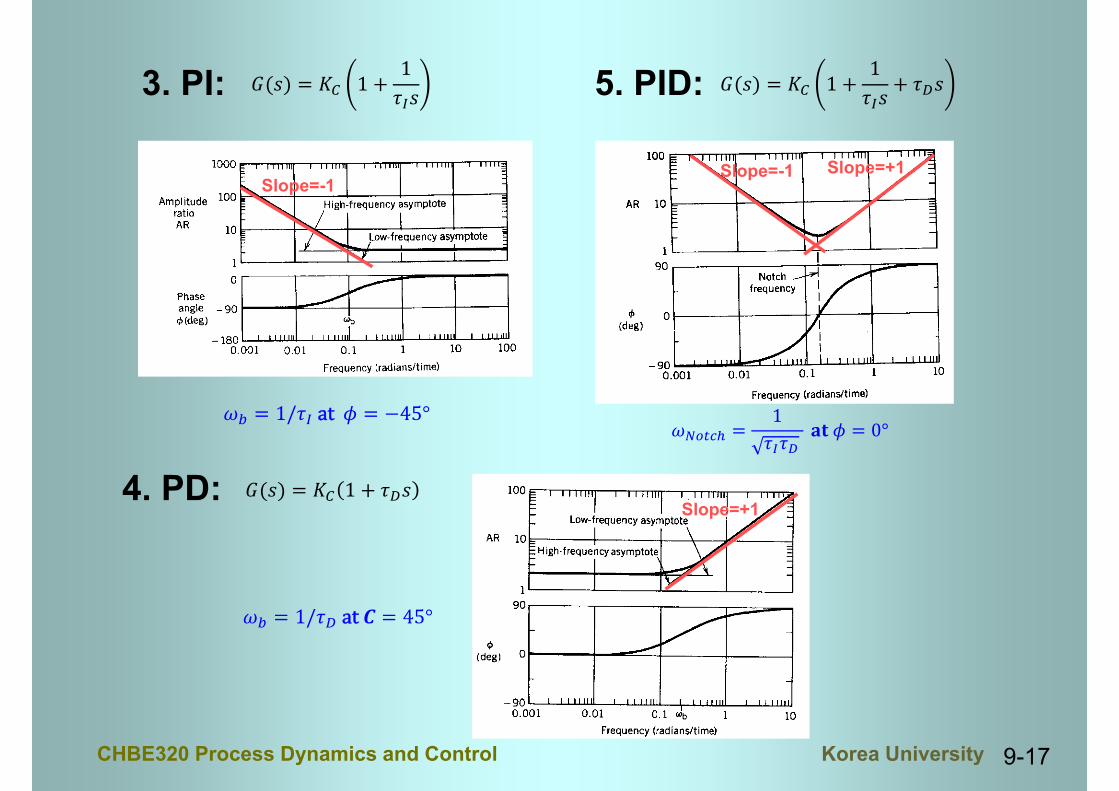
3. PI: 5. PID:

4. PD:

𝐺 𝑠 𝐾 11

𝜏 𝑠 𝐺 𝑠 𝐾 11

𝜏 𝑠 𝜏 𝑠

Slope=-1 Slope=+1

𝜔1

𝜏 𝜏 𝐚𝐭 𝜙 0°𝜔 1/𝜏 at 𝜙 45°

Slope=-1

𝐺 𝑠 𝐾 1 𝜏 𝑠Slope=+1

𝜔 1/𝜏 at 𝑪 45°

9-18CHBE320 Process Dynamics and Control Korea University

NYQUIST DIAGRAM

• Alternative representation of frequency response• Polar plot of ( is implicit)

– Compact (one plot)– Wider applicability of stability

analysis than Bode plot– High frequency characteristics will be

shrunk near the origin.• Inverse Nyquist diagram: polar plot of

– Combination of different transfer function components is not easy as with Nyquist diagram as with Bode plot.

Re

Im

𝜑

𝐺 𝑗𝜔

AR

𝜔 ↑

Nyquist diagram𝐺 𝑗𝜔 Re 𝐺 𝑗𝜔 𝑗 Im 𝐺 𝑗𝜔

𝐺 𝑗𝜔

1/𝐺 𝑗𝜔