Charter School Entry and School Choice:The Case of Washington, D.C.

Maria Marta FerreyraCarnegie Mellon University

Grigory KosenokNew Economic School

July 2, 2012Preliminary and Incomplete

Please do not cite without permission�

AbstractWe develop and estimate a structural equilibrium model of charter school entry and compe-

tition. In the model, households choose among charter, public and private schools. Faced withuncertainty about demand shocks and competitors�actions, charter schools choose whether toenter, exit or relocate based on their expected equilibrium demand. We estimate the model us-ing school-level panel data for Washington, D.C. We use our parameter estimates to investigatethe potential e¤ects of changes in the institutional and demographic environment on charterentry, student sorting across schools, and the distribution of student achievement.

�We thank David Albouy, Stanislav Anatolyev, Steve Berry, Paul Ellickson, Dennis Epple, Fernando Ferreira,Jeremy Fox, Steve Glazerman, Brett Gordon, Bryan Graham, Justine Hastings, Lutz Hendricks, Dan McMillen,Alvin Murphy, Aviv Nevo, Javier Pena, B. Ravikumar, Stephen Ryan, Tim Sass, Holger Sieg, Benjamin Skrainka,Fallaw Sowell, Chris Taber and Matt Turner for useful conversations and comments. We bene�tted from commentsby seminar participants at McMaster and the Federal Reserve Bank of St. Louis, and by session participants at thefollowing conferences: LACEA 2009, Regional Science Association 2010, AEFP 2011, SED 2011, CURE 2011, APPAM2011 and AEA 2012. Ferreyra thanks the Berkman Faculty Development Fund at Carnegie Mellon University for�nancial support. Je¤ Noel and Naomi Rubin DeVeaux from FOCUS, Marni Allen from 21st Century School Fund,Steve Glazerman and the charter school principals we interviewed for this study answered many of our questions oncharters in DC. Special thanks to Prof. Michael Saunders for his assistance with the SNOPT and MINOS algorithms.We thank our research assistants Gary Livacari, Sivie Naimer, Hon Ming Quek, and especially Nick DeAngelis fortheir help with the data collection. Je¤ Reminga assisted us with the computational aspects of the project, and BillBuckingham from the Applied Population Lab at the University of Wisconsin provided Arc GIS assistance. All errorsare ours.

1

1 Introduction

The dismal academic performance of public schools in urban school districts has been a growingconcern in recent decades. Charter schools provide families with additional school choices and areseen by many as a possible solution. Unlike traditional public schools, charter schools are runindependently of school districts by private individuals and associations, and are formed from asuccessful combination of private initiative and the institutional regulations of the policymaker.

Charter schools receive public funding in the form of a per-student stipend. They do nothave residence requirements and if oversubscribed they determine admission by lottery. Charters arefree from many regulations that apply to public schools, but are subject to the same accountabilityrequirements as traditional public schools and are regulated by state laws. Minnesota passed the�rst law in 1991, which has been followed by laws in 40 states and the District of Columbia,all of which di¤er widely in their permissiveness towards charters. The nation�s 5,400 charterscurrently serve 1.7 million students, or about 3 percent of the primary and secondary market.1

While seemingly small, this market share conceals large variation across states and districts.A prospective charter entrant must formulate and present a proposal to the chartering entity.

The proposal, akin to a business proposal, must specify the school�s mission, curricular focus (suchas arts or language), grades served, teaching methods, anticipated enrollment, intended physicalfacilities, and a �nancial plan. In other words, the decision to open a charter school is similarto that of opening a �rm. Like �rms, entering charters seek to exploit a perceived opportunity.For example, in a residence-based system, a low-income neighborhood with low-achieving publicschools may create an opportunity for a charter entrant to serve households not satis�ed with theirlocal public schools. Other example opportunities are middle-class families reasonably well servedby the local public schools but who are interested in a di¤erent type of academic program, or byfamilies who send their children to private schools but are willing to experiment with a charterschool so as to not pay tuition.

In this paper we investigate charter school entry and household choice of school, and studythe case of Washington, D.C. We document the pattern of charter school entry in the city bygeographic area, thematic focus and grade level in order to gain insights about the opportunitiesexploited by charters. Building on these insights we explore how households sort among public,private and charter schools. We also study the e¤ects that the entry, exit or relocation of a schoolhas on others. Finally, we explore how the educational landscape would change in response tochanges in the regulatory framework for charter, public and private schools. This question seemsparticularly relevant given the current focus of federal education policy on charter expansion.2

Addressing these research questions poses several challenges. Consider, for instance, thecase of a new charter entrant. Some families will switch from their current school into the charter,in a process that will shape the peer characteristics of the new school as well as a¤ect the peercharacteristics of the schools previously attended by those children. Since parents care about theirchildren�s peers, this will further a¤ect their choices. In other words, charter school entry triggersequilibrium e¤ects because it leads to a re-sorting of students across schools. Even though thecharter entrant can specify a number of aspects about the new school, such as its thematic focusand educational philosophy, an important characteristic �the composition of the student body �is beyond its control. In this sense charter schools are at a disadvantage with respect to publicschools, which typically have residence requirements and can restrict admission in that way, andwith respect to private schools that can apply their own admission criteria. The second complicating

1See http://www.edreform.com/Fast_Facts/K12_Facts/2The federal �Race to the Top� program favors states with permissive charter legislation. See

http://www2.ed.gov/news/pressreleases/2009/06/06082009a.html for further details.

2

factor in our research questions is the uncertainty faced by schools when making their decisions,both about their own demand and the actions of other schools. This uncertainty is more severe fornew entrants, who may not know their ability to conduct the new enterprise.

Thus, we develop and estimate an equilibrium model of household school choice, charterschool entry and school competition in a large urban school district. In the model, we view acharter entry point as a combination of location (neighborhood), thematic focus and grade level.Since charter funding is connected with enrollment, prospective entrants must be able to forecastthe demand for their services in order to assess their �nancial viability. Hence, we model howprospective entrants predict enrollment and peer characteristics of their student body as a functionof their geographic location, grades served and thematic focus. The prospective entrant enters ornot depending on the expected success of its entry and subsequent viability, which in our frameworkmeans maximizing expected net revenue. We model the entrant as being uncertain about its ownquality at the entry stage.

We estimate the model using a unique and detailed data set from Washington D.C. from2003 to 2007. The data set consists of information for all public, private and charter schools inWashington, D.C. including enrollment by grade, school demographics, focus and pro�ciency ratesin standardized tests. Lacking individual-level data, we augment the school-level data with theempirical distribution of child age, race, poverty status and family income at the block grouplevel, and draw from this distribution in order to calculate the predicted market share and peercharacteristics for each school and grade. Since market shares for public, private and charter schoolsvary widely across grades, our market consists of a grade-year combination. We estimate the modelin three stages corresponding to demand, supply and pro�ciency rates.

We model schools as di¤erentiated products and estimate the demand side of the modelusing an approach similar to Berry et al (1995), henceforth BLP. In particular, we allow for theexistence of an unobserved school-grade-year quality component (such as teacher quality) thathouseholds observe when making choices but the researcher does not. This creates correlationbetween the resulting school peer characteristics and the unobserved quality component, similar tothe correlation between unobserved quality and price in BLP. Unlike price, which is determined bythe company, peer characteristics are determined by aggregate household choices and are similarto the local spillovers in Bayer and Timmins (2007).3 Following Nevo (2000, 2001), we exploit thepanel structure of our data and include school, grade and year �xed e¤ects to capture some of thevariation in the unobserved quality component.

We have chosen to focus on a single, large urban district in order to study the decisions ofprospective entrants that confront the same institutional structure. We study Washington, D.C. forseveral reasons. The city has a relatively old charter law (passed in 1996) that is highly permissivetowards charters. For instance, charter funding in D.C. is more generous than in most other areas,as the per-student charter stipend is equal to the full per-student spending in traditional publicschools, and charters receive a facilities allowance. Moreover, the charter sector has grown rapidlyin D.C., reaching 40 percent of total public school enrollment in 2011.4 The fact that D.C. containsa single public school district facilitates research design and data collection. Finally, the city isrelatively large and contains substantial variation in household demographics, thus providing scope

3General equilibrium analyses of school choice include Benabou (1996), Caucutt (2002), de Bartolome (1990),Epple and Romano (1998), Fernandez and Rogerson (1998), and Nechyba (1999, 2000). Calabrese et al (2006),Ferreyra (2007) and Ferreyra (2009) estimate general equilibrium models. Relative to these prior analyses, oureconometric framework in this paper provides a model of choice among the entire set of schools within a district aswell as a model of charter school entry.

4As of 2010, the districts where this share surpassed 30 percent were New Orleans, Louisiana (61 percent);Washington, D.C. (38 percent); Detroit, Michigan (36 percent); and Kansas City, Missouri (32 percent). Source:http://www.charterschoolcenter.org.

3

for charter entry.Throughout we make several contributions. First, we contribute to the study of charter

school entry. While most of the literature on charters studies their achievement e¤ects5, relativelylittle research has focused on charter entry. The �rst study was conducted by Glohm et al (2005)for Michigan in a reduced form fashion. Rincke (2007) estimates a model of charter school di¤usionin California. In a recent study, Bifulco and Buerger (2012) have studied charter entry in the stateof New York. A theoretical model of charter school entry is developed by Cardon (2003), whostudies strategic quality choice of a charter entrant facing an existing public school. We build onthe foundation established in these papers by modeling intra-district charter school entry decisions,parental choice, and the impact of entrants on public and private school incumbents. Perhapsclosest to our approach is the work of Imberman (2009), who studies entry into a single large urbandistrict in a reduced-form fashion, and Mehta (2012) who studies charter entry in North Carolinain a structural fashion. The most salient di¤erences between our work and Mehta�s are that: a) weendogenize school peer characteristics as equilibrium outcomes determined by household choices;b) while we model charters as being responsive to public schools, we do not model the strategicbehavior of public schools given the lack of evidence for such behavior - as explained below; c) inour model, all charter schools in the economy are available to a given household regardless of itslocation, in accordance with the absence of residence requirements for charter schools.

Second, we contribute to the literature on school choice by studying household choice amongall public, private and charter schools in D.C. while modeling school peer characteristics as theoutcome of household choices. While others have followed a similar approach (Ferreyra 2007,Altonji et al 2011), they have not relied on the full choice set available to households and have notmodeled school unobserved quality.

Third, we match school peer characteristics. While the BLP approach is usually focused onthe parameters that explain the observed market shares, ours must ful�ll the additional requirementof explaining who chooses each school in our data. This exercise, in the spirit of Petrin (2002),provides a natural set of overidentifying restrictions that increase the e¢ ciency of our estimates.

Fourth, we contribute to the computational literature on the estimation of BLP models. Werecast our demand-side estimation as a mathematical programming with equilibrium constraints(MPEC) problem following Dube et al (2011), Su and Judd (2011) and Skrainka (2011). We solvethe problem by combining two large-scale contrained optimization solvers, SNOPT and MINOSin order to minimize computational time and attain the highest possible accuracy in the solution.While Dube et al (2011) and Skrainka (2011) rely on analytical Hessians in order to achieve thesegoals, we rely on an e¢ cient combination of solvers and do not require analytical Hessians, whosederivation is involved and prone to errors. We are currently exploring the use of MPEC to imposeall equilibrium conditions at once rather than in three separate stages. Thus, our research lies atthe frontier of computational methods and estimation.

Finally, we contribute to the entry literature on �rm entry in industrial organization. Areview of this literature is provided in Draganska et al (2008). Most of this literature assumes areduced-form function for demand,6 whereas we specify a full model of household choice of school.In addition, a major focus of that literature is the strategic interaction between entrants and/orincumbents. While we model the strategic interaction among charter schools, we do not modelpublic or private school decision making. The reason is that during our sample period public and

5See, for instance, Bettinger (2005) Bifulco and Ladd (2006), Booker et al (2007, 2008), Buddin and Zimmer(2005a, 2005b), Clark (2009), Hanushek et al (2007), Holmes et al (2003), Hoxby (2004), Hoxby and Rocko¤ (2004),Hoxby and Murarka (2009), Imberman (2009, forthcoming), Sass (2006), Weiher and Tedin (2002), and Zimmer andBuddin (2003).

6A recent exception is Carranza et al, who have a BLP demand-side model.

4

private schools displayed very little entry or exit, a feature that would prevent the identi�cationof a model of strategic decision making for them. Moreover, between 1992 and 2007 the Districtof Columbia Public Schools (DCPS) had seven superintendents. This high turnover, coupled with�nancial instability, suggests that DCPS may not have reacted strategically to charters during oursample period. Since charters experienced more entry, exit and relocation than public or privateschools we model them as being strategic with respect to each other while taking the actions ofpublic and private schools as given. A �nal di¤erence with respect to the entry literature is thatwe rely on panel data, which is quite rare in entry studies. Our panel provides us with variationover time in entry patterns. Perhaps more importantly, by providing us with post-entry outcomes,the panel allows us to learn about the permanent quality of both entrants and incumbents.

We use our parameter estimates to study the e¤ect of changes in the regulatory, institu-tional and demographic environment on charter entry, household sorting across schools and studentachievement. For instance, we explore whether greater availability of building sites for charterswould spur the creation of more charter schools, where these would locate, which students theywould attract, and how achievement would change among the pre-existing schools. Since the au-thorizer plays a critical role in this environment, we examine changes in the authorizer�s preferenceswith regards to focus and school level.

The rest of the paper proceeds as follows. Section 2 describes our data sources and basicpatterns in the data. Section 3 presents our theoretical model. Section 4 describes our estimationstrategy, and Section 5 describes our estimation results. In Section 6 we provide some discussionand describe our intended counterfactuals. Section 7 concludes.

2 Data

Our dataset consists of information on every public, charter and private school in Washington, D.C.between 2003 and 2007. We have focused on the 2003-2007 time period to maximize the qualityand comparability of the data over time and across schools. In addition, 2007 marked the beginningof some important changes in DCPS and hence constitutes a good endpoint for our study.7 Wedirect readers interested in further detail of the dataset to Appendix I.

While public and private schools have one campus each, many charters have multiple cam-puses. Hence, our unit of observation is a campus-year, where a "campus" is the same as a schoolin the case of schools that have one campus each.8 We have 700, 228 and 341 observations forpublic, charter and private schools respectively. Our dataset includes regular schools and speci�-cally excludes special education and alternative schools, schools with residential programs and earlychildhood centers. For each observation we have campus address, enrollment by grade for gradesK through 12,9 percent of students of each ethnicity (black, white and hispanic),10 and percent oflow-income students (who qualify for free or reduced lunch). We also have the school�s thematicfocus, which we have classi�ed into core curriculum, language (usually Spanish), arts, vocationaland others (math and science, civics and law, etc.).

For public and charter schools we have reading and math pro�ciency rates, which is thefraction of students who are pro�cient in each subject based on D.C.�s own standards and assess-

7 In 2007, Michelle Rhee began her tenure as chancellor of DCPS. She implemented a number of reforms, such asclosing and merging schools, o¤ering special programs and changing grade con�gurations in some schools, etc.

8A campus is identi�ed by its name and not its geographic location. For instance, if a campus moves but retainsits name, then it is still considered the same campus.

9We do not include adult or ungraded students, who account for less than 0.6% of total enrollment. We do notinclude students in preschool or prekindergarten because these data are not available for private schools.10Since students from other races (mostly Asian) constitute only 2.26 percent of the total K-12 enrollment, for

computational reasons we added them to the white category.

5

ments. For private schools we have school type (Catholic, other religious and non-sectarian) andtuition by grade.

In Washington, D.C. public schools fall under the supervision of DCPS. Although thereis only one school district in the city, there are many attendance zones. As for charters, until2007 there were two authorizers: the Board of Education (BOE) and the Public Charter SchoolBoard (PCSB). Since 2007, the PCSB has been the only authorizing (and supervising) entity. Theoverarching institution for public and charter schools at the "state" level is the O¢ ce of StateSuperintendent of Education (OSSE).

Enrollment and pro�ciency for public and charter schools comes from OSSE. For publicschools, the source of school addresses and student demographics are the Common Core of Data(CCD) from the National Center for Education Statistics (NCES) and OSSE. Curricular focus forpublic schools comes from Filardo et al (2008). For PCSB-authorized charters, ethnic compositionand low-income status come from the School Performance Reports (SPRs). For BOE-authorizedcharters, the pre-2007 information comes from OSSE, and the 2007 information from the SPRs.CCD provided supplementary data for some charters. For charters, focus comes from the schools�statements on the web, SPRs and Filardo et al (2008).

The collection of public school data was complicated by poor reporting of public schools tothe Common Core of Data during the sample period. Nonetheless, much more challenging was tore-construct the history of location, enrollment and achievement for charter schools, particularlyin the case of multi-campus organizations. The reason is that no single data source contains thefull history of charters for our sample period. Thus, we drew on OSSE audited enrollments, SPR�sfor PCSB-authorized charters, web searches of current websites and past Internet archives, charterschool lists from Friends of Choice in Urban Schools (FOCUS), phone calls to charters that are stillopen and achievement data at the campus level. The resulting campus-level data re�ect our e¤ortsto draw together campus-level information from these di¤erent sources, with the greatest weightgiven to OSSE audited enrollments and achievement data, and the SPRs.

With the exception of tuition, our private school data come from the Private School Survey(PSS) from NCES. The PSS is a biennial survey of private schools. We used the 2003, 2005 and2007 waves. We imputed 2004 data by linear interpolation of 2003 and 2005, and similarly for2006. We obtained tuition information for many private schools from their web sites. Though thisinformation is current, in our empirical application we assume that relative tuitions among privateschools have not changed since 2003 and express tuitions in dollars of 2000.

According to grades covered, we have classi�ed schools into the following grade levels: el-ementary (if grades covered fall within the K-6 range, since most primary schools covered up to6th grade in D.C. during our sample period), middle (if grades covered are 7th and/or 8th, high(if grades covered fall within the 9th - 12th grade range), elementary/middle (if grades span boththe elementary and middle level), middle/high, and elementary/middle/high. This classi�cationfollows DCPS�s criteria and incorporates mixed-level categories (such as middle-high), which arequite common among charters. When convenient, we employ an alternative classi�cation with threecategories: elementary (including all categories that encompass elementary grades: elementary, ele-mentary/middle, elementary/middle/high), middle and high (de�ned similarly). Note that a gradelevel is a set of grades and not a single grade.

2.1 Descriptive Statistics

The population in Washington, D.C. peaked in the 1950s at about 802,000, declined steadily to572,000 in 2000, and bounced back to 602,000 in 2010. During 2003-2007, it is estimated that thepopulation grew from 577,000 up to 586,000 in 2007, although the school-age population declined

6

from 82,000 to 76,000.11 The racial breakdown of the city has changed as well over the last twodecades, going from 28, 65 and 5 percent white, black and hispanic in 1990 to 32, 55 and 8 percentrespectively in 2007. Despite these changes, the city remains geographically segregated by race andincome. Whereas in 2006 median household income was $92,000 for whites, it was only $34,500 forblacks (Filardo et al, 2008).

2.1.1 Basic trends

In 2007, 56 percent of students attended public schools, 22 percent charter schools and 22 percentprivate schools. In what follows, "total enrollment" refers to the aggregate over public, private andcharter schools, and "total public" refers to enrollment in the public system (adding over publicand charter schools).

In national assessments, DC public schools have ranked consistently at the bottom of thenation in recent years. For instance, in the 2011 National Asssessment of Educational Progress,D.C.�s proportion of students in the below-basic pro�ciency category was higher than in all 50states. This might be one of the reasons why charter schools have grown rapidly in DC sincetheir inception in 1996. During our sample period alone, the number of charter school campusesdoubled, from 30 to 60, whereas the number of public and private school campuses declined slightlyas a result of a few closings and mergers (see Figure 1 and Table 2). Over the sample period, 43percent of private schools were Catholic, 24 percent belonged to the Other Religious category and32 percent were nonsectarian.

Even though total enrollment declined during our sample period by about 6,000 students,enrollment in charter schools grew approximately by the same amount (see Figure 2). As a result,the market share of charter schools grew from 13 to 22 percent (see Figure 3) and charter sharerelative to total public enrollment rose from 16 to 28 percent.

As Table 1a shows, student demographics in public and charter schools are quite similar �more than 90 percent black or hispanic and about two thirds low-income. In contrast, in privateschools about 60 percent of students are white and less than a quarter low-income. As Figures 4a-cshow, charters are spread throughout the city except in the northwestern sector, where privateschools have a strong presence. Even though private schools tend to be located in higher-incomeneighborhoods than public or charter schools they are actually quite heterogeneous (see Table 1b).Catholic schools enroll higher fractions of black and hispanic students than other private schools.On average, they also charge lower tuition and are located in less a�uent neighborhoods.

2.1.2 Variation by grade level

As Table 3 shows, most public schools are elementary. Public schools rarely mix levels, but abouta third and three quarters of charter and private schools do, respectively. For instance, half ofCatholic schools�students are enrolled in elementary/middle schools and about 60 percent of thestudents in other private schools are enrolled in elementary/middle/high schools. At every level,private schools tend to be smaller than charter schools, which are in turn smaller than publicschools. High schools are the exception, because the average private (in particular, Catholic) highschool is almost as large as the average public high school. Market share for each school type di¤ersacross grade levels: most public school enrollment corresponds to elementary school students, yetmost of charter and private school enrollment corresponds to higher grades.

11Source: Population Division, U.S. Census Bureau. School-age population includes children between 5 and 17years old. An alternative measure of the size of school-age population is total K-12 enrollment, which also declinedfrom 81,500 to 75,000 students (see Figure 2).

7

Figure 5 o¤ers more detailed evidence on this point. Public school shares peak for elementarygrades; charter school shares peak for middle grades and private school shares peak for high schoolgrades. This is consistent with a popular narrative in D.C. that claims that middle- and high-income parents "try out" their neighborhood public school for elementary grades but leave thepublic sector afterwards.12

While market shares at the high school level changed little over the sample period, theyexperienced greater changes for elementary and middle school grades. Public schools lost elementaryschool students to private and charter schools, yet more striking was their loss of middle schoolstudents to charter schools. This may be explained in part by the fact that at the end of 6th gradepublic school students must switch schools, making 7th grade a natural entry point into a newschool. But, as Figure 6 indicates, it may also be explained by the fact that the supply of charterrelative to public schools is much greater for middle than elementary school grades. While chartersare severely outnumbered by public schools for elementary grades, the di¤erence is much smallerfor middle grades because charter supply grew the most for these grades over the sample period.Moreover, charter middle schools have fewer students per grade than public schools (see Figure 7),a feature that many students may �nd attractive.13 Note in passing that the number of public andprivate high schools is about the same, yet private schools are much smaller.

The popular narrative described above �nds support in Table 4, which shows a decline inthe fraction of white students in middle and high school relative to elementary school while thereverse happens in private schools.14 Note, also, that private high schools are located in higherincome neighborhoods than private elementary or middle schools. Whites are a very small fractionof charter school enrollment in elementary and middle school yet they are an even smaller fractionfor high school. Perhaps as a result of the di¤erences in the student body across grade levels,pro�ciency rates in public schools are higher for elementary than middle or high school grades. Incontrast, charter pro�ciency peaks for middle schools. It then falls for high schools, which enroll aparticularly disadvantaged student population and are located in low-income neighborhoods.

2.1.3 Variation by focus

More than half of charters o¤ered a specialized curriculum (see Table 5a). Among public andprivate schools, only public high schools engage substantially in this practice. Across all types ofschools, language and arts are popular focuses for elementary schools and vocational is popularfor high schools (see Table 5b). Most elementary schools focused on arts are charters that attractvery disadvantaged students and are located in low-income neighborhoods (see Table 6). Languageschools attract high fractions of hispanic students and vocational schools attract very disadvantagedstudents. Although whites attend charter schools at lower rates than public or private schools,charters that o¤er other focuses (such as math and science, special educational philosophies, classics,etc.) attract relatively large fractions of whites. Perhaps for this reason, these schools also tend tohave relatively high achievement.

12Some might claim that white parents leave the District altogether once their children �nish elementary school.As a simple test of this conjecture we calculated the fraction of white children at each age. This fraction declinessteadily between ages 0 and 4, from 19 to 13 percent, but stabilizes around 10 or 11 percent between ages 5 and 18.Thus, white parents appear to leave the District before their children start school, not after elementary school.13This does not necessarily mean that charter schools have smaller class sizes; rather, it may mean that they have

fewer classrooms per grade.14The relatively low percent of white students in middle schools is explained by Catholic schools dominating this

grade level and enrolling a majority of Black students.

8

2.1.4 Relocations, closings and multiple-campus charters

Very few public and private schools opened, closed or relocated during the sample period relativeto the total number of those schools (see Table 2). Charter schools, in contrast, displayed moreaction on those fronts, especially in terms of relocation. It is quite common for charter schools toadd grades over time until completing the grade coverage stated in the charter. Of the 30 campusesthat entered between 2003 and 2006, 26 added grades during the sample period, mostly at highergrades. Hence, many charters �rst open in a temporary location that is large enough to hold theinitial grades, but then move to their permanent facilities once they reach a higher enrollment.

Of the 63 campuses in our sample, 28 pertain to a multi-campus organization, for a total of45 schools. In general, these organizations run multiple campuses in order to serve di¤erent gradelevels.15 The 10 multi-campus schools in our sample accounted for by 46 percent of the charterenrollment during the sample period. Relative to single-campus charters, multi-campus chartersare more likely to focus on a core curriculum, attract slightly higher fractions of black students andachieve greater pro�ciency rates.

2.1.5 Early v. recent entrants

Given our focus on charter entry, an important question is whether the 27 campuses that enteredbefore our sample period ("early entrants") are di¤erent from the 36 campuses that entered duringour sample period ("recent entrants"). As Table 7 shows, recent entrants tend to be smaller andare more likely to serve elementary or middle school. They are also more likely to belong to amulti-campus organization. They enroll greater fractions of white students and are more likely tohave a specialized curriculum. They are located in slightly higher income neighborhoods and enrolllower fractions of low-income students. In other words, it seems as though the charter movementhas been including less disadvantaged students over time. Since these students are likely to enjoyaccess to good public (and perhaps private) schools, in order to reach them charters seem to beo¤ering more curriculum specialization.

To summarize, our data set is unique and draws from a variety of sources. It has not beencompiled or used by any other researcher before. Moreover, it features a rich variation over timeand across schools that will help us identify the parameters of our model.

3 Model

In this section we develop our model of charter schools, household school choice and equilibrium.In the model, the economy is Washington, D.C. There are public, private and charter schools in theeconomy. Each school serves a di¤erent grade level, where a grade level is a collection of grades,and there is a �nite set of grade levels (for instance, elementary, middle and high). The economyis populated by households that live in di¤erent locations within the city and have children whoare eligible for di¤erent grades. For a given household, the school choice set consists of all public,private and charter schools that o¤er the required grade and may be attended by the child.

At each point in time, every neighborhood has a prospective entrant for each grade leveland focus. We use the term �entry point� to refer to a combination of location, grade level andfocus. A prospective charter entrant chooses whether to enter or not, whereas an incumbent charterdecides whether to remain open and relocate, remain open in the same location, or exit. Public andprivate schools react very slowly to changes in the market environment. Hence, the prospective

15For instance, Friendship has two elementary school campuses (Southeast Academy and Chamberlain), one ele-mentary/middle school campus (Woodridge), one middle school campus (Blow-Pierce), and one high school campus(College).

9

entrant takes the locations, grades served, and focus of public and private schools as given (it alsotakes private school tuitions as given).

To make their decisions, both incumbents and potential entrants forecast their enrollmentgiven the competition they face from other schools. To develop this forecast they anticipate house-holds� choices. At the beginning of any given period schools are uncertain about their demandshock yet potential entrants are even more uncertain because they do not know their aptitude atrunning a school.

The model thus has multiple stages: several stages of charter action, and a household choicestage. Since the latter is used in the former, we begin by presenting the model of household choiceof school. Our school choice framework draws from Bayer and Timmins (2007).

3.1 Household Choice of School

The economy includes J schools, each one o¤ering at least one grade. The economy is populatedby households that have one child each. In what follows, we use �household�, �parent�, �child�and �student�interchangeably. Student i is described by (g;D; `; I; "), where:

� g is the grade of the student. Our data covers 13 grades: kindergarten, and grades 1st through12th.

� D is a vector describing student demographics. This vector contains eD elements. In ourempirical application D has 3 rows, each one storing a 0 or 1 depending on whether thehousehold is white, hispanic (default race is black), and non-poor (this indicator equals 1 ifthe student does not qualify for free- or reduced lunch, and 0 otherwise).

� ` 2 f1; :::; Lg is the location of the household in one of the L possible neighborhoods of theschool district. A student�s location determines her geographic distance with respect to eachschool.16

� I is the income of the student�s family.

� " is a vector that describes the student�s idiosyncratic preference for each school.

We use j and t subscripts to denote respectively a school and year. Throughout, if a schoolhas only one campus, j refers to the school; otherwise it refers to the campus. We treat multiplecampus of the same organization as separate entitites because in practice they are run as such. Inwhat follows, we use "school" and "campus" interchangeably. Our data includes J = 281 schoolsand T = 5 years (between 2003 and 2007). A household�s choice depends on several variables thatcharacterize a particular school and that are observed by the household at the time of making itschoice:

� �jt is the set of grades served by the school, often referred to as "grade level." A householdchooses among the set of schools that o¤er the grade needed by its child. This set changesover time, as a school can add or remove grades.

� xijt is the geographic distance from the household�s residence to the school. Since schools canrelocate, distance can vary over time.

16We assume that a student�s location is given and does not depend on her choice of school. For models of jointresidential and school choice, see Nechyba (1999, 2000) and Ferreyra (2007, 2009). In our empirical application,distance is measured as network distance and is expressed in miles.

10

� yj denotes time-invariant school characteristics such as type (public, charter, Catholic, otherreligious, nonsectarian) and focus (core, language, arts, vocational, other). Henceforth, forpresentational clarity, we will refer to yj as �focus.�

� pjgt is tuition. Public and charter schools cannot charge tuition, but private schools can.Private school tuition can vary by grade.17

� Djt represents peer characteristics of the student body at the school. Unlike school char-acteristics yj and pjgt, Djt is the outcome of household choices. It is the average over thevectors D of the students who attend the school and hence has eD elements as well. In ourempirical application, Djt stores percent of white, hispanic and non-poor students. Thesecharacteristics may change over time, as household choices change.

� �pjgt is an unobserved (to us) characteristic of the school and grade. This includes characteris-tics of the teacher such as her responsiveness to parents and her enthusiasm in the classroom;physical characteristics of the classroom, etc.

� �ajgt is an unobserved (to us) characteristic of the school and grade that a¤ects children�sachievement (in contrast, �pjgt a¤ects household satisfaction with the school and grade forreasons other than achievement). Thus, �ajgt captures elements such as teacher e¤ectivenessat raising achievement, the usefulness of the grade curricula to enhance learning, etc.

We de�ne a market as a (grade, year) combination. The size of the market for grade g inyear t is Mgt, equal to the number of students who are eligible to enroll in grade g at time t.

The household indirect utility function is:

Uijgt = �p

jgt + �p

ijgt + "ijgt (1)

where �p

jgt is the baseline utility enjoyed by all the grade g children who enroll in school j attime t, �

p

ijgt is a student-speci�c deviation from the common school-grade utility, and "ijgt is anindividual idiosyncratic preference for (j; g) at t. The baseline utility depends on school and peercharacteristics as follows:

�p

jgt = yj�p +Djt�

p + �pjgt (2)

Here, �p and �p are vectors of parameters. In what follows, we refer to �pjgt as a preference shockfor school j and grade g at time t. A remark on notation is in order at this point. We use a psuperindex to denote some elements of the utility function above, and an a superindex to denoteelements of achievement, to economize on notation when we combine utility and achievement below.

The household-speci�c component of utility is given by:

�p

ijgt = E(Aijgt)�+Diyj~�p+Di �Djt~�+ xijt + ' log(Ii � pjgt) (3)

This component of utility depends on the expected achievement of the student, E(Aijgt), whichis explained below. It also depends on the interaction of yj and Di, which captures the variationin attractiveness of the thematic focus across students of di¤erent demographic groups, and theinteraction of Di and �Djt, which captures the potential variation in preferences for school peercharacteristics across di¤erent demographic groups. In addition, it depends on the distance betweenthe household�s residence and the school and on school tuition.17Recall that our tuition data is for the school year 2010/11, and is expressed in dollars of 2000. Hence, it does

not vary over time in our empirical application.

11

Student achievement Aijgt depends on a school-grade factor common to all students, Qjgt, astudent�s demographic characteristics, the �t of the thematic focus to the student (captured by theinteraction of student demographics and focus below), and a zero-mean idiosyncratic achievementshock �ijgt, which parents do not observe at the time of choosing a school:

Aijgt = Qjgt +Di!a + yjDi~�

a+ �ijgt (4)

As is common in empirical studies of achievement, we include student demographics in this equationbecause factors such as parental education, wealth and income (for which we do not have detailedmeasures and which are likely to a¤ect achievement) vary across racial and ethnic groups. Asdetailed below, the school-grade factor, Qjgt, depends on the thematic focus of the school, peercharacteristics of the student population, and a productivity shock �ajgt for school j and grade g attime t. Since peer characteristic measures are available at the school but not the grade level, wedo not place the subscript g on �D below:

Qjgt = yj�a + �Djt�

a + �ajgt (5)

Substituting (5) into (4), we obtain

Aijgt = yj�a + �Djt�

a +Di!a + yjDi~�

a+ �ajgt + �ijgt (6)

Since parents observe �ajgt but �ijgt has not been realized yet at time they choose a school, theirexpectation of (4) is:

E [Aijgt] = yj�a + �Djt�

a +Di!a + yjDi~�

a+ �ajgt (7)

Substituting (7) into (3), we obtain:

�pijgt = yj�a�+ �Djt�

a�+Di! + yjDi~� +Di �Djt~�+ xijt + ' log(Ii � pjgt) + ��ajgt (8)

where ! = !a�. The coe¢ cient of the interaction of yj and Di is ~� = ~�p+ �~�

a. This interac-

tion captures both the variation in attractiveness of a school�s focus across students of di¤erentdemographic groups ( ~�

p) and the �t between focus and student type in the achievement function

(�~�a).Substitute (2) and (8) into (1) and regroup terms to obtain:

Uijgt = �jgt + �ijgt + "ijgt (9)

where �jgt and �ijgt are de�ned below in (10) and (12). We now turn to a discussion of these terms,beginning with the baseline utility component �jgt:

�jgt = yj� + �Djt�+ �jgt (10)

In this expression, the coe¢ cient of yj captures both household preference for school focus andimpact of focus on achievement: � = �p + ��a. Thus, the model captures an interesting potentialtension between school characteristics that enhance productivity and school characteristics thatattract students. For example, a long school day may enhance achievement, but parents andstudents may not like the longer day. Similarly, the coe¢ cient of �Djt captures both householdpreference for peer characteristics and the impact of peer characteristics on student achievement:� = �p + ��a. The error term in (10) impounds both a preference and a productivity shock:�jgt = �

pjgt+��

ajgt. We will refer to this composite shock as a demand shock or unobserved quality.

Since the demand shock captures elements that a¤ect both utility and achievement, it re�ects the

12

same kind of tension described above. For instance, parents may like the atmosphere created bya teacher in her classroom and the enthusiasm she instills in the students even if these are notre�ected in higher achievement. Following Nevo (2000, 2001), we decompose the demand shock asfollows:

�jgt = �j + �g + �t +��jgt (11)

In this decomposition, the school-speci�c component �j captures elements that are common toall grades in the school and constant over time, such as the school�s culture and average teacherquality. We refer to �j as the permanent quality of the school. The grade-speci�c component �gcaptures elements that are common to a given grade across schools and over time. For instance,retention rates tend to be higher in 9th grade than in any other grade. The time-speci�c component�t captures shocks that are common to all schools and grades and vary over time, such as city-wideincome shocks. We apply the following normalization: E(��jgt) = 0. Hence, �j + �g + �t is themean school-year-grade demand shock, and ��jgt is a deviation from this mean �due, for instance,to the presence of a teacher whose quality is much higher than the school average.

The household-speci�c component of (9) is:

�ijgt = Di! + yjDi~� +Di �Djt~�+ xijt + ' log(Ii � pjgt) (12)

Since the household may choose not to send its child to any school, we introduce an outsidegood (j = 0). This may represent home schooling, dropping out of school, etc. The indirect utilityfrom this outside option is:

Ui0gt = ' log(Ii) + �0gt +Di!0 + "i0gt (13)

Since we cannot identify �0gt and !0 separately from the �jgt terms of the �inside�goods or from!, we apply the following normalizations: �0gt = 0 and !0 = 0.

Let J igt denote the choice set of schools available to household i for grade g at time t. Thischoice set varies over time because of entry and exit of schools that serve that grade, and becausesome schools add or remove grades. Let Xijt denote the observable variables that are either speci�cto the household or to the match between the household and the school: Di, Ii, and xijt. Thehousehold chooses a school from the set J igt in order to maximize its utility (it may also choosethe outside good). Assuming that the idiosyncratic error terms in (9) and (13) are i.i.d. type Iextreme value, we can express the probability that household i chooses school j in grade g at datet as follows:

Pjgt

�yj;y�j; �Djt; �D�jt; �jgt; ��jgt; pjgt; p�jgt; Xijt; �

d�=

exp(�jgt + �ijgt)

exp(' log(Ii)) +

JigtXk=1

exp(�kgt + �ikgt)

(14)where �d refers to the collection of demand-side parameters to be estimated.

Let h (D; I; `; g) be the joint distribution of students over demographics, income, locationsand grades in the economy, and let h(D; I; ` j g) be the joint distribution of demographics, incomeand location conditional on a particular grade. Recall that each location ` is associated with adistance to each school. Given (14), the number of students choosing school j and grade g at timet is equal to: bNjgt = Z

`

ZI

ZD

Pjgt(�)dh(D; I; ` j g) (15)

13

Thus, the market share attained by school j in grade g at time t is equal to:

bSjgt(yj;y�j; �Djt; �D�jt; �jgt; ��jgt; pjgt; p�jgt; �d) = bNjgtMgt

(16)

The total number of students in school j at time t is hence equal to bNjt = Xg2�jt

bNjgt:The resultingdemographic composition for the schools is thus equal to

b�Djt(yj;y�j; �Djt; �D�jt; �j�t; ��j�t; pj�t; p�j�t; �d) =Xg2�jt

bNjgt R RI

RD

DPjgt(�)dh(D; I; ` j g)

bNjt (17)

where the dot in � and p indicates the set of all grades in the corresponding school. In equilibrium,the school peer characteristics taken as given by households when making their school choices, �D;are consistent with the peer characteristics determined by those choices, b�D.

Since we do not have individual-level achievement data, we cannot identify the parametersof the achievement function (4). However, we can derive the following equation for a school�sexpected pro�ciency rate (see Appendix II for details):

qjt = yj�q + �Djt�

q + yj �Djt!q + �qj + �

qt +��

qjt (18)

where the parameters are non-linear functions of the parameters in (4). In this equation, the school�xed e¤ect is a function of the school�s productivity schock and the mean grade productivity shock.The time �xed e¤ect captures changes that a¤ect pro�ciency rates in all schools and grades, suchas modi�cations to the assessment instrument. The error term is a function of school idiosyncraticproductivity shocks and the mean of the idiosyncratic components of performance of the school�sstudents.

3.2 School Supply

Having studied household choice of school, we now turn to the schools. As Table 2 shows, episodesof entry, exit and relocation are much less common among public and private schools than charters,particularly when measured against the number of schools. Hence, there is not enough variationin our data to identify a model of strategic decisions on the part of public or private schools. Atleast during our sample period, these schools seem to have reacted very slowly to changes in theenvironment. Thus, we do not model decision-making on the part of public and private schools;rather, we take their behavior as given from the data. We assume that in any given time period theymake decisions before charters do, and hence charters take public and private schools�decisions asgiven. Of course, it is possible that at some point public and private schools would react to changesin the environment, particularly those created by charter competition. To accommodate for thispossibility, in our counterfactuals we implement simple policy rules for public and private schools,such as closing if enrollment falls below a speci�c threshold and remaining open otherwise.

For these reasons, our supply-side model focuses on charters. We distinguish between po-tential entrant and incumbent charter schools. Both prospective entrants and incumbent chartersseek to maximize expected net revenue, equal to expected enrollment times reimbursement perstudent minus the corresponding costs.18 In particular, charters must forecast their equilibrium

18Reimbursement is the per-student stipend that charters receive in lieu of funding.

14

demand, namely the demand they will face after households re-sort across schools in response tocharter actions.

Below we provide a few institutional details on charter entry to illuminate our modelingchoices regarding entry. Then we describe the information structure facing charters and describethe problem of entrants and incumbents. We �nalize by describing the timing of the entry-exit-relocation game and by describing the equilibrium of the model.

3.2.1 Charter entry: institutional details

If a charter wishes to open in the Fall of year X, it must submit its application by February of(X-1). The Washington, D.C. charter law speci�es that the school�s application must include adescription of the school�s focus and philosophy, targeted student population (if any), educationalmethods, intended location, recruiting methods for students, and an enrollment projection. Theapplicant must also �le letters of support from the community, and specify two potential parentswho will be on the school�s board. In addition, the application must contain a plan for growth �what grades will be added, at what pace, etc.

At the time of submitting its application, the school must provide reasonable evidence thatit will be able to secure a facility. The authorizer evaluates the enrollment projection by consideringthe enrollment in nearby public schools, similar incumbent charters, the size of the school�s intendedbuilding, and how many students the school needs in order to be viable given the expected �xedcosts.

If the application is approved, the charter receives approval notice in April or May of (X-1)and must start negotiations with the authorizer on a few issues, including the building. At the timeof receiving the approval notice, the school should have secured a building, or else the negotiationswith the authorizer will break down. Provided the school secures a building, it then uses thefollowing twelve months to hire and train its prospective leaders, renovate the building (if needed),recruit students and teachers, and get ready to start operating.

Charters are very aggressive in their e¤orts to recruit students. They do neighborhoodsearches, advertise in churches, contact parents directly, post �yers at public transportation stopsand local shops, advertise in local newspapers and in schools that are being closed down or recon-stituted, and host open houses. PCSB also conducts a �recruitment expo�in January and chartersparticipate in it. Word of mouth among parents also plays an important role. This is aided by thefact that a charter�s board must include two parents with children in the school.

Based on its projected enrollment, a charter opening in Fall of X receives its �rst installmentin July of X. This means that any previous down payment on the facilities must be funded througha loan. An enrollment audit is conducted in October of X and installments are adjusted accordingly.

Charters can run surpluses � this is the case, for instance, of charters that are planningto expand in the future. They can also run de�cits, as is the case with schools whose actualenrolment is too low relative to their �xed costs. However, PCSB only tolerates temporary de�cits,and only in the case in which the school is meeting its academic targets. Thus, attracting andretaining students is of utmost importance to charters. Between 2004 and 2010 PCSB received 89applications, of which only 29 were approved.

This long, well-speci�c process motivates the timing of entry-exit-relocation events we de-scribe below. Broadly speaking, schools make entry, exit and relocation decisions �rst, and house-holds choose schools later. Although schools face uncertainty when making choices, the uncertaintyis resolved by the end of the period and households make choices with complete information.

15

3.2.2 Information structure

To illustrate the information problems facing charters, recall that we have de�ned an entry pointfor charters as a combination of location `, focus y and grade level �, and consider a prospectiveentrant for entry point (`; y; �). In order to determine whether to enter or not, she needs toforecast her equilibrium demand taking into account the choice set available to households and thecharacteristics of these choices. However, the entrant faces two sources of uncertainty. First, shedoes not know the choice set available to households because she does not know which other schoolswill enter, exit or relocate. Second, she does not know, for herself or others, a characteristic thathouseholds take into account when choosing schools, namely their demand shock �jgt. This dualuncertainty a¤ects both potential entrants and incumbent charters.

The timing of entry-exit-relocation events we describe below speci�es the information avail-able to a school about others� actions at each point in time and thus addresses the �rst sourceof uncertainty. As for the second source, recall that we have decomposed the demand shock as�jgt = �j + �g + �t + ��jgt. We assume that both prospective entrants and incumbents observe�g because it is time-invariant and common to all schools that o¤er g. We also assume that �tbecomes public knowledge at the begining of period t and is thus observed by prospective entrantsand incumbents. While incumbents observe their permanent quality �j , prospective entrants donot. This captures the notion that a prospective entrant does not know how good she will be at theenterprise of starting and running a school. We assume that if she does enter, she conducts activitiesthat enable her and others to learn her permanent quality - she advertises the new schools, hostsopen houses, hires a principal and teachers, participates in charter fairs, engages in fundraising,etc.

Finally, we assume that at the beginning of t no school observes its school-grade-year devi-ation ��jgt. We assume that �j and ��jgt are independent and that ��jgts are independent acrossgrades for a given school-year. Further, we assume that the distributions of �j and ��jgt are com-mon knowledge, equal to N(��; �

2�) and N(0; �

2��) respectively. For convenience we sometimes refer

to these distributions as N�j and N��jgt respectively. Thus, �jgt is distributed N(�j + �g + �t; �2��)

for all incumbent public, private and charter schools, and N(�� + �g + �t; �2� + �

2��) for potential

charter entrants.In order to forecast her demand for a given period, a charter must integrate over the dis-

tribution of its own ��jgt and that of other schools, and must do so for each grade she serves.Since charters compete with all schools in the city, this is high-dimensional integral. For instance,there were 180 schools o¤ering 1st grade in 2007. Thus, we reduce the computational burden byevaluating other schools���jgt at their mean, equal to �� + �g + �t for entrants and �j + �g + �tfor incumbents.

3.2.3 Charter entrants

Recall we have assumed one prospective entrant per entry point per period. Prospective entrant j inlocation `, grade level � and focus y forms her beliefs about the expected demographic compositionat her school as a solution of the following system of equations

b�Djt = Z�j:t

b�Djt(y; y�j ; b�Djt; b�D�jt; �j�t; ��j�t; p�j�t; �d)dN�j (��; �2�) Yg2�jt

dN��jgt(0; �2��) (19)

where b�D�jt are the beliefs of other schools about their peer characteristics, formed similarly to b�Djt:

16

Given these beliefs, the prospective entrant�s predicted market share for grade g in case ofentering is

EhbSjgt j (`; y; �)i = Z

�jgt

bSjgt(y; y�j ; b�Djt; b�D�jt; �jgt; ��jgt; p�jgt; �d)dN(�� + �g + �t; �2� + �2��) (20)where Sjgt(:) is given by (16) and ��jgt is evaluated at its mean as described above.

Let Rgt denote the reimbursement per student in grade g that a charter school obtains.19

Let V� denote variable costs per student; these may di¤er by grade level, �. Let � be an entry feethat is only paid when entering. Let F`t denote �xed costs which must be paid every year that theschool is open. These may vary by location and time to capture varaition in the main componentof �xed costs, which is the cost of facilities.

The expected revenue net of costs for the prospective entrant j in entry point (`; y; �) is

�e`y�t (�s) =

Xg2�

MgtEhbSjgt j (`; y; �)i (Rgt � V�)� � � F`t + �e`y�t (21)

where �s =���; ��; ���; �; V�; F`t; w

refers to the collection of supply-side parameters to be es-

timated, and �e`y�t is measurement error in the charter school�s pro�ts that is unobserved by theeconometrician. The prospective entrant enters if its expected revenue from entering is higher thanthe utility of not entering, equal to �e0t.

20In the �s vector, parameter w denotes relocation costsand is used below in our model of incumbents. We assume that the error terms �e`y�t and �

e0t are

i.i.d. type I extreme value.In practice, a charter school may serve only a single grade in the �rst year and grow into its

full grade level over time. Our characterization in (21) assumes that the school decides on entrybased on whether it expects non-negative net revenues were it serving its full set of grades fromthe beginning of its operations.

Modeling charters as pro�t-maximizers may not seem appropriate. However, charters cannotrun permanent de�cits and hence must worry about �nancial matters. Moreover, presumably theymust keep their students satis�ed in order to retain them �which suggests that the interests of theschool and the students may be aligned. The concern remains that charters might keep studentssatis�ed without raising their performance. Thus, in future versions we will explore alternativecharter objective functions.

3.2.4 Charter incumbents

An incumbent charter school decides whether it will continue operations, and if so, whether tostay in the current location or move to another one. Moving imposes cost w. Incumbent charter jlocated in `, with focus y and grade level � makes the decision that solve the following problem:

19For a given year, this reimbursement varies across grades. For 2007, the base reimbursement (�foundation�) isequal to $8002.06, and is adjusted by a grade-speci�c factor which is highest for high school and preschool. Thefoundation is adjusted by in�ation every year. In addition, charters in D.C. receive a facility allowance per child,equal to $2,809.59 in 2007.20A potential extension is to have a charter school authorizer that imposes a minimum threshold for net revenue

to internalize the externalities that a failing school imposes on its students.

17

�ijt (�s) = max

8>>>><>>>>:�ijt;stay =

Xg2�

MgtEhbSjgt j (`; y; �)i (Rgt � V�)� F`t + �ijt` if stays in location `

�ijt;move =Xg2�

MgtEhbSjgt j �`0 ; y; ��i (Rgt � V�)� F`0 t � w + �ijt`0 if moves to location `

0

�ijt;exit = �ijt0 if exits

9>>>>=>>>>;(22)

where �ijt` is ideosyncratic shock in the incumbent�s pro�ts that is unobserved by the econometricianbut observable by the incumbent, and the expectations are taken over the distribution of ��jgt.We assume that �ijt` and �

ijt0 follow an i.i.d. type I extreme value distribution.

3.2.5 Timing of entry-exit-relocation events, and equilibrium

Consider time period t. At the beginning of t there are Jt charter incumbents from the previousperiod. Their permanent quality �j is common knowledge as is the set of grade-speci�c demandshocks �g:The entry-exit-relocation game evolves as follows:

Step 1 (Public and Private Schools). At the beginning of t public and private schoolsmake their decisions on entry, exit and relocation. These actions become public knowledge. Thetime-speci�c demand shock �t becomes public knowledge as well.

Step 2 (Expected Pro�ts for Charter Schools). All incumbent charter and potentialentrants calculate the expected pro�t from each possible action and choose the action that maxi-mizes their pro�t. In so doing they take as given the set of public and private schools in the marketfrom Step 1, and the set of incumbents from the previous period. They assume that incumbentsstay at their previous period location, and that no other charter enters. Charter expected pro�tsare given by (21) and (22).

Step 3 (Action Initiation). The potential entrants that have decided to enter and theincumbents that have decided to relocate or exit in Step 2 initiate the corresponding actions. Theirinitiated (i.e., intended) actions become public knowledge. This captures the idea that a charterthat has gained approval from PCSB needs to �nalize the lease of its building, hire teachers, etc.As the charter undertakes these activities, others learn about the charter�s intention to enter.

Step 4 (Action Revision). The actions initiated in Step 3 yield a new market structure,as charters in the market now include those that initiated entry in Step 3, the incumbents thatinitiated relocation or exit in Step 3, and the incumbents that did not initiate any action in Step3 (and thus remain in the same location). The charters that initiated actions in Step 3 recalculatetheir expected pro�t in light of the new market structure. If the re-calculated pro�t from thisstep is lower than the pro�t from the status quo (equal to not entering for intending entrants andnot moving for incumbents), then the charter school revises its decision and withdraws from theinitiated action. All withdrawals become public knowledge. The withdrawals capture the realitythat for some charters the opening process fails at some point.

Step 5 (Iteration): Step 4 is repeated until no charter that initiated actions in Step 3chooses to withdraw from the initiation process.21

Step 6: (Households�school choice) At the end of t, households observe the demandshocks �jgt of all the schools operating in the market, including new entrants and incumbents.Households choose schools based on this information.

To summarize, we model the market as the interaction of schools and households, anddescribe this interaction by the multistage game speci�ed above. In the �nal stage of the game,households sort across schools given the supply of schools. In equilibrium, the resulting school peer

21Step 4 can only be repeated a �nite number of times.

18

characteristics are consistent with households�choices, and no household wishes to alter its choice.The other stages of the game represent the strategic interaction of the schools. In particular, weassume that they play Perfect Bayesian Equilibrium. In equilibrium, every school forms consistentbeliefs about the equilibrium strategies of competing schools, households�choices and the resultingpeer compositions. Every charter school chooses the strategy that maximizes its payo¤ conditionalon these beliefs.

4 Data and Estimation

To estimate the model, we proceed in three stages. First, we estimate demand-side parameters �d.Second, we estimate supply-side parameters �s. Third, we estimate pro�ciency rate parameters �q.Below we describe the data used to estimate the model and each of the three estimation stages.

4.1 Data

The data required to estimate the model consists of enrollment shares for schools in each market;school characteristics; information on the joint distribution of household residential location, incomeand demographic characteristics for each market; and number and characteristics of the schools thatenter, exit and relocate each year during the sample period.

Our data includes 65 markets (13 grades times 5 years) and J =281 campuses, for a total ofJD=1,269 school-year observations and JS=8,112 school-grade-year observations. Since we do nothave direct information on the number of children eligible for each grade in each year, AppendixIII describes how we estimate market size. Based on school-grade-year enrollment and grade-yearmarket sizes we then calculate the vector S with 8; 112 school-grade-year enrollment shares.

Recall that we have data on the following school characteristics: governance (public, charter,Catholic, other religious, private non-sectarian), location, grade span, focus, peer characteristics(percent of students of each ethnicity and low-income status), and tuition (by grade) for privateschools. Some school characteristics change over time while others remain constant. Location variesfor schools that move during the sample period. Grade span varies for a number of schools thateither add or drop grades over the period. Entry and exit of schools o¤ering a given grade as wellas changes in grade span of the existing schools a¤ects the composition of households�choice sets.Thematic focus is constant over time and across grades within a school. For a given school, peercharacteristics change over time. Pro�ciency rates vary over time.

In the model, the economy is a collection of locations. For the sake of our demand estimation,a location ` consists of a Census block group (there are 433 block groups in D.C.), and each locationis populated by households characterized by the grade that their child must attend (K, 1, ... 12),race (black, white or hispanic), income, and poverty status (whether they qualify for free- orreduced-lunch or not). Ideally, we would observe the joint distribution of child grade requirement,race, parental income and child poverty status at the block group level, and we would observe itfor each year between 2003 and 2007. Since this is not the case, Appendix IV describes how weuse 2000 Census data to non-parametrically estimate this joint distribution for year 2000 �rst andthen for every year in our sample period.22

22Our estimation combines school-level data with Census aggregate household data. These two sources are generallyconsistent except in one aspect, namely the percent of low-income students. Schools report that approximately 60percent of their students receive free- or reduced- lunch, yet only 46 or 47 percent of school-age children qualify forit according to the Census. The discrepancy is worse for elementary schools than high schools. In future versionswe will explore either dropping poverty status information altogether, or in�ating the model�s predicted percent lowincome students by a grade-level multiplier in order to match the data.

19

Once we have this joint distribution, we randomly draw ns = 100 households for eachmarket.23 In the absence of data on the distribution of child age by grade, we assume two ages pergrade (ages 5 and 6 in kindergarten, 6 and 7 in �rst grade, etc.), and we draw an equal number ofchildren of each age per grade.

At �rst we attempted to construct school choice sets for households in every location andgrade that included all the charter and private schools o¤ering that grade but only the publicschools assigned to that location given attendance zone boundaries. Attendance zones are largerfor middle and high schools than for elementary schools, and boundaries changed once during oursample period (in 2005). Appendix IV describes how we assigned each block group to an elementary,middle and high school attendance zone in each year. However, based on our resulting assigmentand other sources (Filardo et al 2008, and phone conversations with DCPS sta¤), we concluded thatthe actual assignment mechanism in D.C. was based on residential location only to a limited extentand was not systematic across the District. Thus, we opted for modeling the choice set availableto a household interested in a given grade as the full set of schools o¤ering that grade - namely, asthough there were open enrollment in public schools. In future versions we will explore intermediatesolutions between a pure residence-based assignment and a pure open-enrollment system.

4.2 Demand Estimation

In the �rst stage of estimation we estimate the utility function parameters that explain the observedmarket shares and the school choices made by households. We formulate household choice ofschool as a discrete choice problem and estimate preference parameters using an approach based onBLP. An important point of departure relative to BLP is our inclusion of school endogenous peercharacteristics in household utility. BLP allows for endogeneity in prices, yet prices are determinedby producers. Our endogenous characteristics, in constrast, are the outcome of aggregate householdchoices. They are similar to the local spillovers in Bayer and Timmins�(2007) sorting model.

To estimate the demand parameters �d, we must �rst calculate the predicted school-grade-year market shares and school-year demographic compositions. Consider the ns children eligibleto attend grade g in year t in our . The predicted enrollment in school j, grade g at time t is

Njgt =Mgt

ns

nsXi=1

Pjgt

�yj;y�j; �Djt; �D�jt; �jgt; ��jgt; pjgt; p�jgt; Xijt; �

d�

(23)

Denote by Xt the union of the Xijt sets. Based on the above, the predicted enrollment share for

(j; g) at t is equal to bSjgt = bNjgtMgt

: Thus, the school�s predicted enrollment is equal to Njt =Pg2�jt

Njgt,

and predicted school peer characteristics are as follows:

b�Djt =Pg2�jt

�Mgt

ns

� nsPi=1DiPjgt (�)

Njt(24)

where Di are household i�s demographic characteristics. In the expressions above, the scaling factorMgt

ns adjusts for di¤erences in actual size across markets even though we randomly draw the same(ns) number of children for each market.

We assume that E��Djt j Xt

�= b�Djt. Thus, observed peer characteristics �Djt are di¤erent

from their expected value due to sampling (and perhaps measurement) error:

23Note that ns = 100 implies 6,500 household draws in total since we have 65 markets. When we began the project,RAM limitations prevented us from using larger values of ns. We have overcome some of those limitations now andwill explore sensitivity of our results to greater values of ns.

20

�Djt =b�Djt + ujt (25)

Since parents observe the unobserved (to us) school characteristics ��jgt and make ther decisions

accordingly, the school demographic composition �Djt that results from household choices is cor-related with ��jgt. Let Z

Xjgt be a row vector of L

X instruments, and ZDjt be a row vector of LD

instruments. In our preferred speci�cation, LX = 332 and LD = 137. Recall that JX = 8; 112 andJD = 1; 269: Vertically stacking all observations yields matrices ZX , with dimension JX by LX ,and ZD, with dimension JD by LD.

Following BLP and Nevo (2000, 2001), we assume that the school-grade-year deviation froma school�s unobserved mean quality is mean independent of the corresponding instruments:

E���jgt j ZXjgt

�= 0 (26)

In addition, we assume that the sampling error in student demographics is mean independent ofthe corresponding instruments:

E�ujt j ZDjt

�= 0 (27)

Recall that vector ujt has eD elements, one for each peer characteristic. Hence, these conditionalmoments yield the following (LX + LD � eD) moment conditions:

Eh�ZXjgt

�0��jgt

i= 0 (28)

Eh�ZDjt�0udjt

i= 0 (29)

where udjt indicates the sampling error in a speci�c demographic characteristic d (for instance, inpercent white students). Vertically stacking all observations yields vectors and rearranging elements

yields vectors �� and u with JX and�JD � eD� rows respectively. The �rst set of JD rows in vector

u correspond to the �rst demographic characteristic; the second set set to the second demographiccharacteristic, and so forth for thefD demographics. In order to interact the sampling error foreach demographic characteristic with every instrument in ZD we introduce matrix eZD, which isblock diagonal and repeats ZD along the diagonal for a total of eD times. We use the term "sharemoments" to refer to (28) and "demographic moments" to refer to (29).

The sample analogs of (28) and (29) are the following vectors:

�X(��) =1

JXZX

0 ��� (30)

�D(��; �d) =

1

JDeZD 0 � u

with LX and�LD � eD� elements respectively.

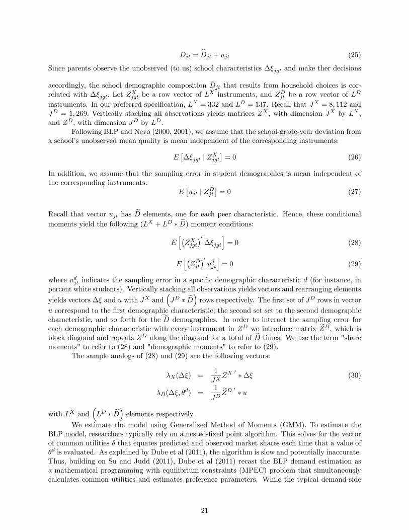
We estimate the model using Generalized Method of Moments (GMM). To estimate theBLP model, researchers typically rely on a nested-�xed point algorithm. This solves for the vectorof common utilities � that equates predicted and observed market shares each time that a value of�d is evaluated. As explained by Dube et al (2011), the algorithm is slow and potentially inaccurate.Thus, building on Su and Judd (2011), Dube et al (2011) recast the BLP demand estimation asa mathematical programming with equilibrium constraints (MPEC) problem that simultaneouslycalculates common utilities and estimates preference parameters. While the typical demand-side

21

BLP approach would consist only of the share moments, we augment our MPEC objective functionby including the demographic moments as well.

Since ujt is sampling error, it is independent of the elements upon which households basetheir choices. One such element is ��jgt. Hence, we assume E

�ujt j ��jgt

�= 0 for all the grades

in school j, and write our MPEC problem as follows:

min��; �d

��X(��)

�D(��; �d)

�0 �VX 00 VD

� ��X(��)

�D(��; �d)

�(31)

s:t:

S = S(��; �D; �d)

where the sample moments are de�ned as in (30). The MPEC algorithm simultaneously searchesover values for �� and �d; given values for these, it calculates the predicted market shares and peercharacteristics. The constraint of the MPEC problem ensures that the observed enrollment sharesS match the predicted enrollment shares S given values for the preference parameters, demandshocks and observed peer characteristics.

In order to implement optimal GMM we must calculate the optimal weighting matrix. Thus,we �rst solve our �rst-stage MPEC problem, described by (31) for arbitrary VX and VD matrices.

Let�~�d;�~�

�be the this problem�s solution. Based on �rst-stage results we constuct the optimal

weighting matrix for the second-stage MPEC and solve the following problem:

min��; �d

��X(��)

�D(��; �d)

�0 �WX 00 WD

� ��X(��)

�D(��; �d)

�(32)

s:t:

S = S(��; �D; �d);

with the elements of the weighting matrix given by

WX =

(1

(JX)2

hZX : � (�~� � e0LX )

i0�hZX : � (�~� � e0LX )

i)�1(33)

WD =

(1

(JD)2MD 0 �MD

)�1

where :� denotes element-by-element matrix multiplication, and matrixMD is of size JD�(LD� eD).The content of this matrix is

MD =�ZD: � (~u1 � e0

LD) ::: ZD: � (~u eD � e0

LX)�

where ud d = 1; :::; ~D, is the size JD vector of sampling error for demographic characteristic d andeT is a vector with ones of size T . This formulation assumes that the ��jgt shocks are independentacross schools and grades and over time, but allows for correlation among sampling errors of percentwhite, hispanic and non-poor for a given school-year. In future versions we will allow ��jgt to becorrelated over time for a given school-grade.

Let��d;��

�be the solution to this problem. To estimate the standard errors of our

parameter estimates �d, we �rst calculate the derivatives of the sample moments �S and �D with

respect to �das follows:

22

Q@�X =1

JXZX

0 � @S�1(S; �D; �

d)

@(�d)0(34)

Q@�D =1

JD

��ZD 0

�� @

b�D(��; �d)@(�d)0

where the vector function S�1(S; �D; �d) = �� is the solution of the share equation. The variance-

covariance matrix of �dis then equal to

V (�d) =

(�Q@�XQ@�D

�= �WX 00 WD

� �Q@�XQ@�D

�)�1Finally, the decomposition of the demand shock in (11) suggests the inclusion of school-,

grade- and time-�xed e¤ects in the utility function. Since the school-speci�c dummy variablescapture both the value of school characteristics that do not vary over time, yj�, and the school-speci�c mean of unobserved quality, �j in (10), we apply a minimum-distance procedure as in Nevo(2000, 2001) in order to estimate � and �j separately. Recall that J = 281 is the number ofschools in the data. Denote by B the J � 1 vector of school-speci�c dummy variables estimatedby GMM; by y the J � Y vector of time-invariant characteristics (governance and focus), and by �the J � 1 vector of school-speci�c demand shocks. From (10) and (11) we can see that our school�xed e¤ects capture the total e¤ect of time-invariant characteristics: B = y� + �. Following Nevo(2000, 2001), we assume that E

��j j yj

�= 0, which allows us to recover the estimates of � and �

as � =�y0V �1B y

��1y0V �1B B and � = B � y� respectively, where B is the vector of school dummy

coe¢ cients contained in �dand estimated through GMM, and VB is the variance-covariance matrix

of these estimates.

4.3 Supply estimation

In the second stage of estimation we match the entry, exit and relocation decisions of charters inorder to estimate the supply parameters �s =

���; ��; ���; �; V�; F`t; w

. In our empirical appli-

cation we consider L = 40 locations or neighborhood clusters,24 Y = 5 focuses and K = 3 gradelevels for a total of 600 entry points. Over our sample period, these amount to 3,000 instances ofpossible charter entry, exit or relocation.25 Yet as Table 2 illustrates there are only 30 entries, 3exits and 20 relocations over our sample period. Such low number of episodes would not enable usto calculate the distribution of outcomes from the entry-exit-relocation game. Hence, we approx-imate this distribution by calculating the logit probability of these outcomes conditional on theobserved market structure. We will then check the accuracy of this approximation through MonteCarlo simulations of the steps of the game at the estimated values of �s.

We estimate �s through Maximum Likelihood Estimation (MLE). Denote by ~It the infor-mation available to the econometrician on market structure for period t. The likelihood functionis then

~L (�s) =TYt=1

248<:CtYj=1

Pr�djt = djt j ~It

�9=;8<:

LY`=1

YYy=1

KY�=1

Pr�d`y� = d`y� j ~It

�9=;35 (35)

24A neighborhood cluster is a collection of Census tracts that is often used by DC planning agencies to proxy fora �neighborhood.�While D.C. includes 188 Census tracts, it only has 40 neighborhood clusters. Thus, the use ofneighborhood clusters rather than Census tracts or block groups eases computational burdens.25 In our data there is at most one entry per entry point and year.

23

where T is the number of periods in the data and Ct is the number of charter incumbents at thebeginning of period t.

As for the probabilities inside ~L (�s), Pr�djt = djt j ~It

�is the conditional probability that

incumbent j chooses action djt given the observed market structure. Recall that the number ofpossible actions for the incumbent is equal to L + 1, as the incumbent can operate in any of theL locations or exit. We assign ` = 0 to the option of exiting. Thus, the probability that theincumbent chooses location djt, djt 2 f0; 1; 2; :::; Lg is given by

Pr�djt = djt j It

�=

exp���ijtdjt

�~It

��LP=0

exp���ijt`

�~It

�� (36)

where ��ijt`�~It

�is the mean pro�t of incumbent j at time t if it locates in `. The pro�t is given

by (22). The other set of probabilities in ~L (�s), Pr�d`�y = d`�y j ~It

�, describes entry behavior in

each entry point (`; y; �). The probability of entering is given by

Pr�d`�y = enter j ~It

�=

exp���e`y�(

~It)�

1 + exp���e`y�(

~It)� (37)

where ��e`y�(~It) is the mean pro�t from (21). Since the probabilities in (37) and (36) also depend on

the demand side parameters �d, we use our estimates of these parameters when conducting MLE.

4.4 Pro�ciency Rate Estimation, and Summary

Although we cannot identify the parameters of the achievemet function, 26 we can identify theparameters of the expected pro�ciency rate in (18), which is related to the observed pro�ciencyrate �qjt as follows:

�qjt = yj�q + �Djt�

q + yj �Djt!q + �qj + �

qt +��

qjt + v

qjt (38)

Here, the error term is the addition of the a school-year unobserved shock on pro�ciency��qjt and school-year sampling or measurement error in pro�ciency rates v

qjt. Since ��

qjt may be

correlated with the demand shocks ��jgt observed by parents when choosing schools, �Djt is likelyto be correlated with �qjt, thus requiring the use of instrumental variables. Denote by Z

Q the setof instruments used to this end.

In the equation above, it is not possible to estimate the coe¢ cient on school time-invariantcharacteristics �q and the school �xed e¤ects �qj . This issue is similar to the one we face whenestimating utility function parameters, and we therefore solve it in a similar way.

To summarize, our estimation approach proceeds in three stages. First, we exploit orthog-onality conditions related to demand shocks and demographic sampling errors in order to estimateutility function parameters. Second, we match charter school decisions in order to estimate supply-side parameters. Third, we estimate the pro�ciency rate parameters.

26Aggregate achievement data, such as average test scores, would allow us to identify a subset of parameters of theachievement function. Detailed notes are available from the authors.

24

4.5 Instruments

For the identi�cation of the demand-side and pro�ciency rate parameters, the main concern is theendogeneity of peer characteristics in the utility and pro�ciency rate functions. Much of this concernis alleviated by the inclusion of school-, grade- and time-speci�c dummy variables following thedemand shock decomposition in (11). However, the concern remains that when households chooseschools, they observe the school-grade-time speci�c deviation ��jgt, which we do not observe. Thisinduces correlation between student peer characteristics �Djt, which are an outcome of householdchoices, and ��jgt.

To address this correlation, we instrument for �Djt using the observed peer characteristicsof "similar but distant" schools. The idea behind this instrument is that the peer characteristics of"similar" schools are correlated, but their grade-year speci�c valuations are not if the schools are"distant." Consider, for instance, two elementary public schools located in neighborhoods with thesame average household income, but four miles apart from each other. The fact that the schoolsare located in similar neighborhoods means that they will attract observationally similar students,but because they are far away, grade-speci�c idiosyncrasies (such as who teaches a speci�c grade)will not be correlated.

We de�ne "similarity" as follows. For charters belonging to a multi-campus organization,similar schools are other charters in the same organization. The idea is that campuses of thesame organization may be perceived as belonging to the same �brand� yet their speci�c grade-year valuations are not correlated because the campuses operate independently and serve di¤erentgrade levels. This idea is similar to that of Nevo (2000, 2001), who instruments for the price of abrand in one market with the price of the same brand in other, distant markets. For single-campuscharters, similar schools are other charters with the same focus and grade level.27 For publicschools, similar schools are other public schools that serve the same grade level and are located inneibghborhoods with similar demographics (in particular, similar average household income). Forprivate schools, similar schools are other private schools of the same type (Catholic, other religiousor nonsectarian), grade level, tuition range, and neighborhood demographic characteristics. To beconsidered "distant", an elementary school must be farther away than 2 miles; a middle schoolmust be farther away than 2.5 miles, and a high school must be farther away than 3 miles.28

Note that the set of similar-but-distant schools for a given school-grade-year varies acrossgrades within a school. For instance, the set of similar-but-distant schools for the 4th grade ofAdams Elementary School is 2004 is the set of schools that are "similar" to Adams, as describedabove, and o¤er 4th grade. This set may not be the same as for Adams�s 5th grade since gradecon�guration varies substantially across schools and even over time for some schools. This isparticularly true of charters, for which entry, relocations and grade additions a¤ect the set ofsimilar schools.

Thus, our ZX matrix contains the following instruments: percent white, percent hispanicand percent low-income in the �ve most similar-but-distant schools;29 interactions between grade-level dummies and the demographics of the most similar-but-distant school; and campus-, grade-and year-level dummies.30

27We also use this similarity notion for multi-campus charters for the years in which they only have one campusopen.28Filardo et al (2008) report median distance traveled from children in each neighborhood cluster to school, by

grade level. Most median distances fall below the thresholds we are using.29We gave to each school in the set of similar-but-distant schools an index that was increasing in distance and

similarity. Hence, the schools from the set that were most similar yet located at the greatest distance were includedas instruments.30To avoid highly collinear instruments, we regressed each one on all the others and eliminated those for which

more than 85 percent of their variation could be explained by the other instruments.

25

As for ZD, the sampling error in school-year average peer characteristics must be meanindependent of its columns. Since characteristics of the schools that a¤ect households�choices arevalid instruments, matrix ZD contains campus dummies.31

Finally, matrix ZQ used for the pro�ciency rate estimation is similar to ZX and containsthe following instruments: percent white, percent hispanic and percent low-income in each of �vemost similar-but-distant schools, and campus- and year-level dummies.

4.6 Identi�cation

We �rst discuss the identi�cation of demand-side and pro�ciency rate parameters, and then ofsupply-side parameters. Lack of individual achievement data prevents us from identifying theachievement function parameters (�a; �a; !a; ~�

a). The parameters of the baseline component of

utility, (�; �) in equation (10), are identi�ed. Parameters � capture both the household preferencefor peer characteristics and the impact of peer characteristics on student achievement: � = �p+��a.In addition to �a not being identi�ed, � is not identi�ed either as discussed below. Since we cannotidentify �a, the individual components of � are not identi�ed. A similar reasoning applies to� (baseline utility of time-invariant school characteristics) and its individual components. Giventhat the default demographic group is (black, low income), � and � re�ect black and low-incomehouseholds�preferences. Parameters � are identi�ed by the extent to which black and low-incomestudents mix with students from other races and economic status in schools, and parameters �are identi�ed by the variation in the fraction of black and low-income students among schools ofdi¤erent types and focuses.

Parameters�~�; ~�; ; !; '

�of the household-speci�c component of utility in (12) are identi-

�ed. Parameter ! is the utility from the portion of achievement due to a student�s own characteris-tics: ! = !a�. While ! is identi�ed, !a is not as discussed above. Hence, the weight of achievementon utility � is not identi�ed either. Since !0 is normalized to zero for the outside good and thedefault demographic group is (black, low income), ! is the di¤erence in relative utility of goingto school versus not going for other demographic groups relative to the default. It is identi�ed bythe variation across demographic groups in the fraction of school-age children who are enrolled inschool.

Parameter ~� is identi�ed. Parameter ~� is the the coe¢ cient on the interaction betweenhousehold demographics and school focus. It is a weighted average of the household�s preferencefor the school focus and focus impact on achievement: ~� = ~�

p+�~�

a. While ~� is identi�ed, neither

� nor ~�aare identi�ed, as we saw above. Thus, ~�

pis not identi�ed either. From the perspective of

counterfactual analysis of the impact of policies on school choice, identi�cation of the componentsof �; � and ~� is not required.

Parameters ~� and ~� are the di¤erence between white, hispanic and non-poor householdsrelative to default households in preferences over peer characteristics and time-invariant schoolcharacteristics. These parameters are identi�ed by the extent to which these groups mix withothers in schools and by their and by their enrollment patterns across schools of di¤erent typesand focuses. Parameter is the disutility of geographic distance between the household�s residenceand the school, and is identi�ed by the geographic distribution of households and schools andthe extent to which schools�demographic composition matches that of nearby neighborhoods. In

31We use a set of 137 campus dummies rather than the full set of 281 campus dummies in ZD. The reason isthat the remaining orthogonality conditions are redundant and lead to an ill-posed second stage MPEC problem.Applying a greedy algorithm, we removed the set of campus dummies that most contributed to a high conditionnumber for the WD matrix in the second stage MPEC problem. After removing those dummies and re-running the�rst stage, the second-stage WD matrix has a condition number of the order of 1e4.

26

general, variation in school type, focus and location is critical to the identi�cation of preferenceparameters. Parameter ' is the utility from the consumption of all other goods. It is identi�ed bythe variation in household income, school tuition and peer characteristics across schools.

School �xed e¤ects �j are identi�ed by having multiple grades and years per school (allof them are included in the estimation). Since �0gt = 0 for the outside good, �j represents thedi¤erence in utility from attending school j relative to the outside good. Grade �xed e¤ects �g areidenti�ed by having multiple schools and year per grade. Since �rst grade is the omitted category,�g is the di¤erence in the utility of going to school rather than choosing the outside good for gradeg relative to �rst grade. Year �xed e¤ects �t are identi�ed by having multiple schools and gradesper year. Since 2003 is the omitted year, �t is the di¤erence in the utility of going to school ratherthan choosing the outside good in year t relative to 2003.

A formal condition for identi�cation is that the matrix of derivatives of the sample moments

with respect to the parameters, Q@� =

�Q@�XQ@�D

�have full rank. Evaluated at our parameter

estimates, this matrix indeed has full rank.32

Pro�ciency rate parameters in (38)are identi�ed by the variation in focus across schools andin student demographics across schools and over time. Having multiple observations per school andmultiple observations per year allows us to identify the school and year �xed e¤ects, respectively.

On the supply side, the charter entry fee � is identi�ed by the frequency of entry in thedata. The �xed cost F`t is identi�ed by the variation in entry patterns across locations and overtime holding entrant and demand characteristics constant. Variable costs V� are identi�ed by thepattern of entry by grade level holding other things constant. Moving costs w are identi�ed bythe frequency of moves. Finally, the parameters of the distribution of demand shocks, ��; �� and��� are identi�ed by the frequency of entry, exit and moves in the data, and by the distribution of�j for the actual entrants (which we estimate based on demand-side �xed e¤ects). Note, however,that we cannot estimate these parameters entirely based on the distribution of the estimated �j�sfor the actual entrants because they parameters pertain to the distribution of unobserved schoolquality for all charters, including those that do not enter.

4.7 Computational Considerations

Currently we have estimated the demand side of the model. Obtaining these estimates involvessolving the MPEC problem in (32). This is a problem with 8,446 unknowns �334 parameters in�d (including 281 campus �xed e¤ects) and 8,112 elements in the �� vector �and 8,112 equalityconstraints (equalities between predicted and observed market shares).

We coded the MPEC problem in MATLAB using the code from Dube et al (2011) as astarting point. Rather than code analytical �rst-order and second-order derivatives for the MPECproblem, we chose to use the automatic di¤erentiation capabilities in TOMLAB�s TomSym package(included in the Base module). This enabled us to experiment with di¤erent model speci�cationsand instruments by only modifying the objective function and the constraints, and leaving TomSymto recompute the derivatives. Automatic di¤erentiation can be memory intensive, especially forsecond-order derivatives, but our problem size and our choice of the SNOPT and MINOS solversavailable from TOMLAB made it e¢ cient and easy. SNOPT and MINOS require only analytic �rst

32The condition number for this matrix is in the order of 1e3. We ran multiple speci�cations and computed thismatrix for each one. Based on a QR decomposition of this matrix we eliminated the parameters that created highcollinearity among the columns of the matrix. The parameters we eliminated are in fact those for which we wouldexpect weak identi�cation given our data. This process allowed us to arrive at our preferred speci�cation.

27

order derivatives. In contrast, Dube et al (2011) supplied second-order derivatives to the KNITROsolver and used the Interior/Direct algorithm.

We used both the SNOPT and MINOS solvers in the following manner: we ran a fewhundred major iterations of SNOPT to establish the basis variables (the variables of interest forthe optimization problem) and to approach a local minimum, and then handed over the problemto MINOS in a "warm-start" fashion to converge to the local optimum. This combination allowsus to exploit the virtues of each solver and solve the problem in the most e¢ cient way. Broadlyspeaking, SNOPT is better suited for a large numbers of unknowns, but makes progress only bychanging its limited-memory approximation of the full Hessian of the Lagrangian between majoriterations. Once it gets to the point at which it no longer updates the Hessian approximation, itstops making progress. In contrast, MINOS works with the exact Lagrangian and can also makemany updates to a full quasi-Newton approximation of the reduced Lagrangian. Hence, MINOScan make progress even when SNOPT cannot provided the size of the problem is not too large.At the same time, MINOS only works well if started su¢ ciently close to a local minimum. Hence,SNOPT starts the problem with the full set of unknowns, quickly solves for �� and establishes�d as the basis variables. After having reduced the size of the problem, it hands the optimizationproblem over to MINOS.

This approach proved fast and accurate, allowing us to obtain results with 5 or 6 decimaldigits of precision.33 For our preferred speci�cation, SNOPT-MINOS took 10.5 hours for the �rststage MPEC problem, and 3.5 hours for the second stage MPEC problem on a workstation with a2.8 GHZ AMD Opteron 4280 processor with 64GB of RAM.34 The computational time comparesfavorably with what Dube et al (2011) and Skrainka (2011) report for BLP problems, particularlytaking into account that our problem has complicating features relative to straightforward BLP. The�rst is that our objective function includes demographic moments in addition to share moments.The second is that we have a relatively large number of products (schools) relative to the number ofmarkets (grade-years). In a typical industrial organization context there are many markets relativeto products. This gives rise to a sparser Jacobian, which in turn speeds up performance (see Dubeet al 2011 for a discussion of how the speed advantage of MPEC declines as the sparsity of theJacobian falls). The third complicating feature is the presence of some very small market shares,an issue related to the large number of schools relative to the number of students.

5 Estimation Results

Currently we have estimated the demand side of our model. Our demand-side model �ts the dataon peer characteristics very well. Across 1,269 school-year observations, the correlation betweenobserved and predicted percent white, percent hispanic and percent non-poor students equals .96,.96 and .94 respectively. Most of our parameters estimates are signi�cant and of the expected sign,as explained below.

33The precision is determined by a combination of the algorithm�s optimality tolerance, the condition number of theJacobian at the optimum, and the size of the dual variables. We used an optimality tolerance of 1e-6 and re-scaledthe problem as needed to ensure that the dual variables had order unity. The output logs report the Jacobian�scondition number, and these were checked. SNOPT and MINOS work best if the objective function gradients, theJacobian of the constraints, and the dual variables are of order unity. This is easily achieved by multiplying theobjective function and constraints by constant factors. We found that the solvers are 3-5 times faster by employingthis scaling.34The workstation had many cores, but the SNOPT-MINOS solvers are single-threaded and so use only one core.

The solvers had a peak memory consumption of 10GB when the derivatives were symbolically computed, and thenworked with 5GB of RAM. On our 64GB workstation we could therefore run multiple jobs at once from multiplestarting points.

28

Table 8 presents our parameter estimates. The "baseline utility" column displays the esti-mates of the parameters in equation (10). Given the parameterization of household demographics,these parameters represent the preferences of black, low-income households. The remaining columnspresent estimates of the parameters in equation (12), which re�ect di¤erences in the preferencesof white, hispanic and non-poor households with respect to the preferences of black, low-incomehouseholds. These interaction e¤ects are crucial to the �t of the data: without them, the correla-tions between observed and predicted peer characteristics are of the order of 0.6.35 At the sametime, the variation in our data is not enough to identify some of the parameters, most notably theinteraction between the constant term and household demographics which capture heterogeneityacross demographic groups in the value of being enrolled in school versus consuming the outsidegood.

In terms of school type, blacks, whites and non-poor households are indi¤erent betweenpublic and charter schools, but hispanics strictly prefer charters. All households prefer publicover Catholic schools, although whites have a less negative valuation of Catholic schools than theother groups. All households prefer public over other religious private schools. While blacks areindi¤erent between public and private non-sectarian schools, other households prefer public overprivate non-sectarian schools. These �ndings are robust to a number of alternative speci�cations.

As for focus, all households prefer core over language with the exception of the non-poor,who prefer language. Whites and hispanics prefer arts over core and blacks are indi¤erent betweenthe two, but non-poor households prefer core. Blacks are indi¤erent between vocational and core,but hispanics and non-poor prefer core. All households prefer core over �other� focus with theexception of whites.

While blacks are indi¤erent between increasing the fraction of white and black students inthe school, all other groups prefer an increase in the fraction of white rather than black students.Increasing the fraction of hispanics rather than blacks is preferred only by hispanics, althoughwhites are more favorable to hispanics than blacks. The estimates imply that whites prefer tomix with other whites rather than blacks or hispanics; hispanics prefer to mix with hispanics orwhites but not blacks; and blacks are indi¤erent about mixing with whites rather than other blacksbut strictly prefer to mix with other blacks rather than hispanics. Estimated preferences overpeers�races are thus aligned with those in Hastings et al (2009), who documents that parents havepreferences for peers of the same demographics. Our estimates also echo those in Bayer et al (2007),who documents households�preference to self-segregate based on demographics.

As for non-poor students, no demographic group prefers to mix with them rather thanlow-income students, although non-poor students are less disinclined to mixing with other non-poor students. These �ndings are robust to a number of alternative speci�cations.While somewhatsurprising, they might be explained by the fact that we are also controlling for tuition. It ispossible that controlling for tuition, households prefer to have an increase in poor rather thannon-poor students.

Finally, the coe¢ cient on distance is negative and signi�cant indicating that householdsprefer shorter travels to school. To the extent that there is actually some residence-based assignmentto public schools in D.C., this coe¢ cient may attribute to preferences what is really an institutionalrequirement. Without data on these requirements, though, it is hard to tease out these di¤erentelements. The coe¢ cient on the consumption of other goods is positive and signi�cant, indicatingnegative sensitivity with respect to price. In future versions we will investigate the variation inprice (tuition) elasticity among households, and in cross-price elasticities among schools.

Thus, while households have relatively similar preferences for school type, their preferencesover school focus are quite di¤erent. Their preferences over peer characteristics are also heteroge-

35Results from this and alternative speci�cations are available from the authors upon request.

29

neous �whereas all attach positive value to having greater fraction of whites in the school (withblacks being indi¤erent between additional blacks and whites), only hispanics attach positive valueto having a greater fraction of Hispanics. These parameter estimates help explain some of theenrollment patterns observed in the data. For instance, Table 6 shows a signi�cant presence ofhispanics in language schools. However, this presence is apparently not due to their preferencefor language relative to core (their disutility from language relative to core is robust across manydi¤erent speci�cations). Rather, it seems driven by the fact that most language schools are char-ters, which is the most preferred school type for hispanics, and that they attract a large fractionof hispanic students.

To summarize, our estimates show substantial variation in household preferences over schoolcharacteristics. This variation creates an entry opportunity for charters, as di¤erent householdsprefer di¤erent focuses and peer characteristics. In future versions we will study the distribution ofhousehold willingness to pay for these characteristics to develop further insights on these preferences.

6 Discussion, Extensions and Intended Counterfactuals

For all its richness, our data is limited in some regards. These limitations, most of which are due tothe unavailability of the corresponding data, have forced us to ignore certain institutional featuresof charter schools in our model. First, we do not observe school capacity or e¤ective demand (i.e.,the number of students who apply to the school). Thus, our model cannot capture a distinctiveaspect of charter schools, namely that they must randomize access when oversubscribed. A relatedconcern is that our school �xed e¤ects could be capturing not only unobserved school quality butalso school capacity, and hence might be estimating high "quality" for schools that are simply largeand have high market shares.

Second, we do not observe the complete set of charter applications submitted to PCSBfor authorization; we only observe the applications that were approved and entered the market.During the �rst part of our sample period there were two charter school authorizers in D.C., theBOE and the PCSB (see Section 2). Some have suggested that the BOE tended to authorizelower-quality applicants (Buckley and Schneider 2007). This, in turn, might have led prospectiveentrants to "shop" authorizers at the beginning of the sample period, and could have been re�ectedin a change in the distribution of school-speci�c quality when PCSB became the sole authorizer.Third, in reality charters choose whether to be single- or multi-campus organizations in a choicethat probably resembles a store chain�s decision to open a new franchise. We plan on investigatingthis issue further.

We will use our parameter estimates to conduct some counterfactuals. First, we will studythe response of charter entry and student sorting to changes in per-student funding for charterschools. Given that real estate is a prime concern for charters, we are particularly interested inexamining the consequences of raising the facilities allowance for charters. On a related note, we willstudy the response of greater access to facilities (represented as a lower �xed cost in some locations).DCPS has made some vacant public school buildings available for charters (Filardo et al, 2008). Aspublic school enrollment continues to decline the supply of facilities for charters should increase.Moroever, in recent years charters have had increasing access to "incubator facilities" where theyare housed for a few years until they move to their permanent locations. We can capture the greateraccess to initial facilities through lower entry fees and/or lower �xed costs for certain locations.

While many states provide free transportation for children (even for those attending privateor charter schools), D.C. does not provide any busing for public, private or charter school children.Thus, the provision of publicly-funded busing could alter household choices signi�cantly. It couldalso alter the geographic pattern of charter entry and location. Furthermore, the charter landscape

30

is heavily in�uenced by the preferences of the authorizer. Hence, changes in these preferences arelikely to a¤ect charter entry and student sorting. For instance, some claim that the authorizertoday is less interested in approving vocational charters than it was a few years ago. Thus, it isof interest to study whether students would be less likely to attend charters if they were not ofthe exact focus that they prefered. Similarly, in recent years charter entry has been concentratedat the elementary and middle school level. The question, then, is whether lowering entry costs forcharter high schools would encourage their entry.

DCPS has undergone important changes in recent years. These changes include schoolclosings, consolidations, re-con�guration of grades, and adoption of specialized curricula. We willstudy the e¤ect of these changes on charter entry and student sorting. More generally, we will studythe e¤ects of a more responsive DCPS. Even if DCPS did not react much to charters during oursample period, given their loss of market share to charters over the past few years, public schoolswill be forced to respond at some point. Thus, we will study the e¤ects of alternative responses.

Washington, D.C. is home to a publicly-funded voucher program for private schools. Sincethe recipients of these vouchers are demographically similar to the students attending charters(Filardo et al, 2008), an expansion of the current program is likely to a¤ect charter schools. Ourmodel allows us to study this issue. A related issue is the general response of private schools tocharters. While private schools did not seem particularly responsive during the sample period, atsome point they might begin to respond, particularly if new charter entrants continue to targeta more a­ uent, less disadvantaged student population. The question of interest is how privateschools would compete in that context.

Finally, one of the main demographic changes a¤ecting most urban school districts in theUnited States is the loss of school-age children. Thus, we will explore the response of charters andhousehold to exogenous demographic shocks that change the potential enrollment in the city as awhole or that change the income distribution of the families with school-age children.

From a methodological perspective, we will explore the use of MPEC to impose all equi-librium constraints at once rather than in three separate stages. In addition, we have beguninvestigating the consequences of relaxing the BLP assumption that market shares are observedwithout error. While this is a plausible assumption in markets with many consumers relative tothe number of products, it may not be so in markets such as ours that consist of approximately6,000 children per grade-year and at least 40 or 50 schools per grade. Currently we assume thatmarket shares are observed without error but school demographics are observed with error. Thus,we have designed an estimator for the case in which both shares and demographics are observedwith error. We are exploring the performance of this estimator in ongoing work.

Finally, Filardo et al (2008) contains tabulations of aggregate data for D.C. during oursample period that we are interested in matching in the estimation. For instance, they reportthe average distance to school traveled by children in each neighborhood cluster in D.C. Since ourmodel predicts this distance, we can match it to the observed data. Matching additional datamight be necessary given the lack of institutional information regarding school assignments. Forinstance, we have noticed that the predicted distance to school with our current estimates is toohigh relative to that reported in Filardo et al (2008), most likely as a consequence of not knowingpublic school assignment rules. Matching distance traveled to school would solve this problem and,in so doing, would help us produce more credible counterfactuals.

7 Conclusion

In this paper we have developed a model of charter school entry and household choice of school andhave devised an estimation strategy for the model. We estimate the model using a unique dataset

31

for Washington, D.C., which incorporates information on all public, charter and private schools inD.C. between 2003 and 2007. Since we rely on an equilibrium framework, we are able to capturethe fact that peer characteristics are the outcome of parental choices, and that parents, in turn,respond to this composition when making choices. We model charter entrants as being uncertainabout their school-speci�c quality, and making their entry decisions based on their expected revenuegiven the opportunities available to households.

Understanding the decisions made by charters and households helps us predict their re-sponses to policy changes. Through our counterfactuals we will analyze alternative policies facingcharter schools. Today, charter schools not only provide children with additional school choices butalso provide researchers with new evidence on school management methods, educational curricula,and a number of aspects in which charters can diverge from public schools by virtue of the freedomsthat have been granted to them. Thus, in future research we will further explore the innovationand competition induced by charters in the education market.

References

[1] Altonji, Joseph, C. Huang and Chris Taber (2011). �Estimating the Cream Skimming E¤ect ofPrivate School Vouchers on Public School Students.�Working Paper, University of Wisconsin-Madison.

[2] Bayer, Patrick and Christopher Timmins (2007). �Estimating Equilibrium Models of SortingAcross Locations" Locations,�Economic Journal, 117(March), 353-374.

[3] Bayer, Patrick, Fernando Ferreira, and Robert McMillan (2007). �A Uni�ed Framework forMeasuring Preferences for Schools and Neighborhoods,� Journal of Political Economy, vol.115, No. 4, 588-638.

[4] Benabou, Roland (1996). �Heterogeneity, Strati�cation and Growth: Macroeconomic E¤ectsof Community Structure,�American Economic Review, 86, 584�609.

[5] Berry, Steven, James Levinsohn, and Ariel Pakes (1995). �Automobile Prices in Market Equi-librium,�Econometrica, 63, 841-890.

[6] Bettinger, Eric P. (2005). �The E¤ect of Charter Schools on Charter Students and PublicSchools," Economics of Education Review, 24, 113-147.

[7] Bifulco, Robert and Christian Buerger (2012). The In�uence of Finance and AccountabilityPolicies on Charter School Locations. Working Paper, Syracuse University .

[8] Bifulco, Robert and Helen F. Ladd (2006). "The Impacts of Charter Schools on StudentAchievement: Evidence from North Carolina," Education Finance and Policy, 1 (1), 123-138.

[9] Booker, Kevin, Scott Gilpatric, Timothy Gronberg, and Dennis Jansen (2007). "The Impact ofCharter School Attendance on Student Performance," Journal of Public Economics, 91 (5/6),849-876.

[10] Booker, Kevin, Scott Gilpatric, Timothy Gronberg, and Dennis Jansen (2008). "The E¤ectof Charter Schools on Traditional Public School Students in Texas: Are Children Who StayBehind Left Behind?," Journal of Urban Economics, 64 (1), 123-145.

32

[11] Buckle, Jack and Mark Schneider (2007). Charter Schools: Hope or Hype?, Princeton andOxford: Princeton University Press.

[12] Buddin, Richard and Ron Zimmer (2005a). "Is Charter School Competition in CaliforniaImproving the Performance of Traditional Public Schools?," RAND Working Paper.

[13] Buddin, Richard and Ron Zimmer (2005b). "Student Achievement in Charter Schools: AComplex Picture," Journal of Policy Analysis and Management, 24 (2), 351-371.

[14] Calabrese, Stephen, Dennis Epple, Thomas Romer, and Holger Sieg (2006). "Local PublicGood Provision: Voting, Peer E¤ects, and Mobility,", Journal of Public Economics, 90, 6-7(August): 959-81.

[15] Cardon, James H. (2003). "Strategic Quality Choice and Charter Schools," Journal of PublicEconomics, 87 (3), 729-737.

[16] Carranza, Juan Esteban, Jean-Francois Houde and Robert Clark (2011). �Dynamic Entry andFirm Recon�guration in Canadian Gasoline Markets.�Working Paper, ICESI University.

[17] Caucutt, Elizabeth (2002). "Educational Policy when There Are Peer Group E¤ects� SizeMatters," International Economic Review, 43, 195�222

[18] Clark, Damon (2009). "The Performance and Competitive E¤ects of School Autonomy," Jour-nal of Political Economy, 117 (4), 745-783.

[19] de Bartolome, C. (1990). "Equilibrium and Ine¢ ciency in a Community Model with PeerGroup E¤ects," Journal of Political Economy, 98, 110�133.

[20] Downes, Thomas A. and Shane M. Greenstein (2006). "Understanding the Supply Decisionsof Nonpro�ts: Modelling the Location of Private Schools," RAND Journal of Economics, Vol.27(2), Summer, pp. 365-390.

[21] Draganska, Michaela, Michael Mazzeo, and Katja Seim (2009). "Beyond Plain Vanilla: Model-ing Joint Product Assortment and Pricing Decisions," Quantitative Marketing and Economics,7(2), 105-146.

[22] Draganska, Michaela, Sanjog Misra, Victor Aguirregabiria, Pat Bajari, Liran Einav, PaulEllickson, Dan Horsky, Sridhar Narayanan, Yesim Orhun, Peter Reiss, Katja Seim, VishalSingh, Raphael Thomadsen, and Ting Zhu (2008). "Discrete choice models of �rms�strategicdecisions," Marketing Letters, 19, 399�416.

[23] Dubé, Jean-Pierre, Jeremy Fox, and Che-Lin Su (2011). "Improving the Numerical Perfor-mance of BLP Static and Dynamic Discrete Choice Random Coe¢ cients Demand Estimation,"Forthcoming, Econometrica.

[24] Dunne, Timothy, Shawn Klimek, Mark Roberts and Daniel Yi Xu (2009). "Entry, Exit andthe Determinants of Market Structure," NBER Working Paper 15313.

[25] Epple, Dennis and Romano, Richard (1998). "Competition Between Private and PublicSchools, Vouchers, and Peer-Group E¤ects". American Economic Review, March, 88(1), pp.33-62.

33

[26] Fernandez, Raquel and Richard Rogerson (1998).: "Public Education and Income Distribu-tion: A Dynamic Quantitative Evaluation of Education-Finance Reform," American EconomicReview, 88, 813�833.

[27] Ferreyra, Maria M. (2007). "Estimating the E¤ects of Private School Vouchers in Multi-DistrictEconomies". American Economic Review, 97 (3): 789-817.

[28] Ferreyra, Maria M. (2009). "An empirical Framework for Large-Scale Policy Evaluation, withan Application to School Finance Reform in Michigan". American Economic Journal: Eco-nomic Policy, vol. 1 no. 1: 147�80.

[29] Filardo, Mary, Marni Allen, Nancy Huvendick, Ping Sung, David Garrison, Margery Turner,Jennifer Comey, Barika Williams and Elizabeth Guernsey (2008). "Quality Schools andHealthy Neighborhoods: A Research Report." Available at www.brookings.edu.

[30] Glomm, Gerhard, Douglas Harris, and Te-Fen Lo (2005). "Charter school location," Economicsof Education Review, 24, 451�457.

[31] Hanushek, Eric A., John F. Kain, Steven G. Rivkin, and Gregory F. Branch (2007). "Char-ter School Quality and Parental Decision Making With School Choice," Journal of PublicEconomics, 91 (5/6), 823-848.

[32] Hastings, Justine, Thomas J. Kane and Douglas O. Staiger (2009). "Heterogeneous Preferencesand the E¢ cacy of Public School Choice." Working Paper, Brown University.

[33] Holmes, George M., Je¤ DeSimone, and Nicholas G. Rupp (2003). "Does School Choice In-crease School Quality?," NBER Working Paper No. 9683.

[34] Hoxby, Caroline M. (2004). "Achievement in Charter Schools and Regular Public Schools inthe United States: Understanding the Di¤erences," Dept. of Economics, Harvard University,mimeo.

[35] Hoxby, Caroline M. and Jonah E. Rocko¤ (2004). "The Impact of Charter Schools on StudentAchievement," Dept. of Economics, Harvard University, mimeo.

[36] Hoxby, Caroline M. and Sonali Murarka (2009). "Charter Schools in New York City: WhoEnrolls and How They A¤ect Their Students�Achievement," NBER Working Paper No.14852.

[37] Imberman, Scott A. (forthcoming). "Achievement and Behavior of Charter Students: Drawinga More Complete Picture," Review of Economics and Statistics.

[38] Imberman, Scott A. (2009). "The E¤ect of Charter Schools on Achievement and Behavior ofPublic School Students", Working paper, University of Houston.

[39] Mazzeo, Michael (2002). "Product Choice and Oligopoly Market Structure," RAND Journalof Economics, vol. 33, No. 2, summer, 1-22.

[40] Mehta, Nirav (2012). Competition in Public School Districts: Charter School Entry, StudentSorting, and School Input Determination. Working Paper, Western Ontario University.

[41] National Alliance for Public Charter Schools (2010). "How State Charter Laws RankAgainst the New Model Public Charter School Law," January, downloaded fromwww.publiccharters.org.

34

[42] Nechyba, Thomas J. (1999). School Finance Induced Migration and Strati�cation Patterns:The Impact of Private School Vouchers," Journal of Public Economic Theory, v. 1, pp. 5�50.

[43] Nechyba, Thomas J. (2000). "Mobility, Targeting and Private School Vouchers," AmericanEconomicReview, 90, 130�146.

[44] Nevo, Aviv (2000). "Mergers with Di¤erentiated Products: The Case of the Ready-To-EatCereal Industry," RAND Journal of Economics, vol. 31, No. 3, Autumn, 395-421.

[45] Nevo, Aviv (2001). "Measuring Market Power in the Ready-To-Eat Cereal Industry," Econo-metrica, v. 69, No. 2 (March), 307-342.

[46] Petrin, Amil (2002). "Quantifying the Bene�ts of New Products: The Case of the Minivan,"Journal of Political Economy, vol. 110, 705-729.

[47] Rincke, Johannes (2007). "Policy di¤usion in space and time: The case of charter schools inCalifornia school districts," Regional Science and Urban Economics, 37, 526�541.

[48] Sass, Tim R. (2006). "Charter Schools and Student Achievement in Florida," Education Fi-nance and Policy, 1 (1), 123-138.

[49] Seim, Katja (2006). "An Empirical Model of Firm Entry with Endogenous Product-TypeChoices, " RAND Journal of Economics, vol. 37, No. 3, Autumn, 619-640.

[50] Skrainka, Benjamin (2011). A Large-Scale Study of the Small Sample Performance of Random

[51] Coe¢ cient Models of Demand. Working Paper, University of Chicago.

[52] Su, Che-Lin and Kenneth L. Judd (2011). "Constrained Optimization Approaches to Estima-tion of Structural Models," Forthcoming, Econometrica.

[53] Suzuki, Junichi (2010). "Land Use Regulation as a Barrier to Entry: Evidence from the TexasLodging Industry," Working Paper, University of Toronto.

[54] Weiher, Gregory R. and Kent L. Tedin (2002). "Does Choice Lead to Racially DistinctiveSchools? Charter Schools and Household Preferences," Journal of Policy Analysis and Man-agement, 21 (1), 79.

[55] Zimmer, Ron and Richard Buddin (2003). "Academic Outcomes," in Charter School Opera-tions and Performance, RAND, pp. 37-62.

35

36

TABLE 1a

Demographics and Achievement at Public, Charter and Private Schools

All Schools Public Schools Charter Schools Private Schools

Avg. 10th

pctile.

90th

pctile. Avg.

10th

pctile.

90th

pctile. Avg.

10th

pctile.

90th

pctile. Avg.

10th

pctile.

90th

pctile.

Pct. White 17.20 0 78.71 7.61 0 30.6 2.80 0 5.00 56.12 0 85.1

Pct Black 73.84 15.67 100 81.89 37.47 100 89.69 68.00 100 38.16 7.27 99.21

Pct. Hispanic 8.96 0.24 26.00 10.49 0 34.47 7.51 0 26.00 5.72 0 10.92

Pct. Low Income 56.88 3.24 87.63 64.68 27.44 88.56 70.47 50.30 95.00 23.74 1.48 76.58

Reading Prof. 41.34 15.47 72.97 41.18 14.55 77.52 41.93 25.32 63.39 n/a n/a n/a

Math Prof. 41.55 13.51 73.98 41.25 12.80 75.27 42.66 21.05 67.16 n/a n/a n/a

Tract Income $61,970 $27,400 $136,600 $55,600 $27,400 $104,800 $43,400 $20,800 $65,600 $95,000 $32,700 $139,700

Notes: The unit of observation is a campus-year. “Reading Prof.” is the percent of students who are proficient in Reading. “Tract income” is the average

household income in the Census tract where the school is located. Pct. Low Income for private schools is imputed as described in Appendix I. Proficiency data is

not available for private schools. Weighted statistics; weight = Fall enrollment.

37

TABLE 1b

Demographics of Private Schools by Private School Type

Catholic Other Religious Nonsectarian

Avg. Pct. White 42.91 66.91 67.52

Avg. Pct Black 49.02 30.39 27.84

Avg. Pct. Hispanic 8.07 2.70 4.64

Avg. Tuition $7,800 $19,700 $20,900

Tract Income $76,000 $120,500 $102,800

Notes: See Table 1a.

38

TABLE 2

School Openings and Closings

Public Schools Charter Schools Private Schools

Year Total Opened Closed Moved Total Opened Closed Moved Total Opened Closed Moved

2003 142 0 0 0 30 3 0 0 70 0 0 0

2004 143 2 1 0 39 10 1 2 68 0 2 0

2005 142 0 1 0 46 8 1 6 70 2 0 2

2006 137 0 5 4 54 9 1 7 67 1 4 0

2007 136 0 1 4 60 6 0 5 68 0 2 3

Notes: Each cell indicates number of campuses. A school’s opening year is its first year of operation; a school’s closing year is the year following the last. A

school is counted as moving in year X if its address in X is different from its address in (X-1).

TABLE 3

Grade Levels at Public, Charter, and Private Schools

Public Schools Charter Schools Private Schools

Percent

(1)

Pct. of

Students

(2)

Avg.

Enrollment

(3)

Percent

(4)

Pct. of

Students

(5)

Avg.

Enrollment

(6)

Percent

(7)

Pct. of

Students

(8)

Avg.

Enrollment

(9)

Elementary 68.57 55.02 277 42.11 27.69 192 17.30 8.14 116

Elementary/Middle 4.29 4.97 400 21.05 22.76 315 51.91 36.03 171

Middle 14.43 16.46 393 11.84 13.59 334 0.59 0.32 39

Middle/High n/a n/a n/a 6.14 7.41 352 5.87 5.39 226

High 12.71 23.55 639 14.91 21.16 413 7.33 18.63 626

Elem./Middle/High n/a n/a n/a 3.95 7.38 545 17.01 31.71 459

Notes: The unit of observation is a campus-year. For instance, on average during the sample period 68.57 percent of public schools are elementary, 4.29 are

elementary/middle, etc. Among public school students, on average 55.02 percent attend elementary schools, 4.97 attend elementary/middle schools, etc.

39

TABLE 4

Demographics and Achievement by School Type and Level

Public Schools Elementary Middle High

Avg. Pct. White 9.10 5.22 6.32

Avg. Pct. Black 79.63 86.62 82.92

Avg. Pct. Hispanic 11.28 8.16 10.77

Avg. Pct. Low Income 68.09 67.74 53.94

Avg. Pct. Proficient Reading 46.90 37.13 31.50

Avg. Pct. Proficient Math 46.17 36.51 34.05

Avg. Tract Hh. Income $54,300 $55,700 $58,400

Charter Schools

Elementary Middle High

Avg. Pct. White 3.87 3.93 0.84

Avg. Pct. Black 86.67 88.03 93.70

Avg. Pct. Hispanic 9.46 8.04 5.46

Avg. Pct. Low Income 74.48 67.44 66.17

Avg. Pct. Proficient Reading 41.93 48.88 34.89

Avg. Pct. Proficient Math 40.78 49.70 37.00

Avg. Tract Hh. Income $44,600 $44,700 $41,200

Private Schools

Elementary Middle High

Avg. Pct. White 58.74 36.70 68.33

Avg. Pct. Black 38.52 56.39 26.29

Avg. Pct. Hispanic 2.73 6.91 5.39

Avg. Pct. Low Income 28.12 41.91 11.32

Avg. Tract Hh. Income $82,800 $75,050 $109,700

Note: “elementary”, “middle” and “high” correspond to the three-type category described in the text.

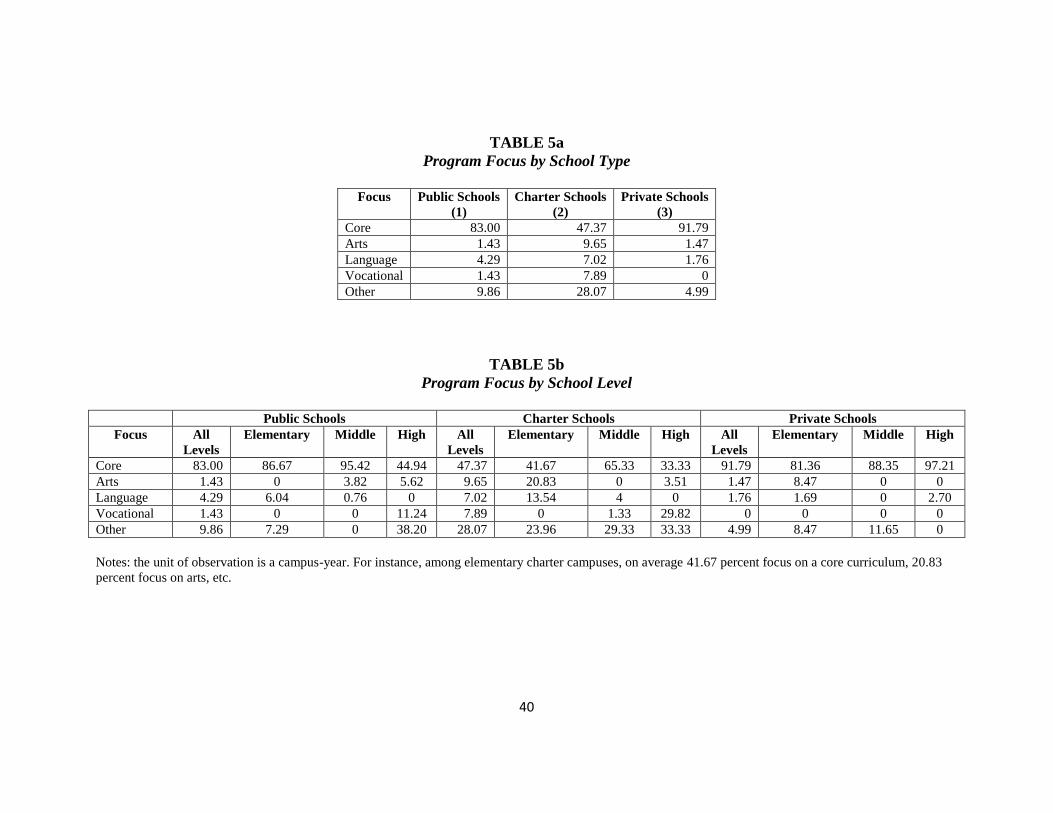
40

TABLE 5a

Program Focus by School Type

Focus Public Schools

(1)

Charter Schools

(2)

Private Schools

(3)

Core 83.00 47.37 91.79

Arts 1.43 9.65 1.47

Language 4.29 7.02 1.76

Vocational 1.43 7.89 0

Other 9.86 28.07 4.99

TABLE 5b

Program Focus by School Level

Public Schools Charter Schools Private Schools

Focus All

Levels

Elementary Middle High All

Levels

Elementary Middle High All

Levels

Elementary Middle High

Core 83.00 86.67 95.42 44.94 47.37 41.67 65.33 33.33 91.79 81.36 88.35 97.21

Arts 1.43 0 3.82 5.62 9.65 20.83 0 3.51 1.47 8.47 0 0

Language 4.29 6.04 0.76 0 7.02 13.54 4 0 1.76 1.69 0 2.70

Vocational 1.43 0 0 11.24 7.89 0 1.33 29.82 0 0 0 0

Other 9.86 7.29 0 38.20 28.07 23.96 29.33 33.33 4.99 8.47 11.65 0

Notes: the unit of observation is a campus-year. For instance, among elementary charter campuses, on average 41.67 percent focus on a core curriculum, 20.83

percent focus on arts, etc.

41

TABLE 6

Student Demographics and Achievement by School Level and Program Focus

a. Elementary Schools

Core

(1)

Arts

(2)

Language

(3)

Other

(4)

Pct. Public 87.80 0 61.22 74.76

Pct. Charter 7.80 98.60 26.53 18.10

Pct. Private 4.40 1.40 0.12 7.15

Avg. Percent White 9.86 1.12 12.18 20.68

Avg. Percent Black 82.01 94.92 38.12 74.99

Avg. Percent Hispanic 8.13 3.96 49.70 4.33

Avg. Percent Low Income 68.01 85.24 72.06 46.87

Avg. Pct. Proficient in Reading 45.06 36.77 50.54 59.06

Avg. Pct. Proficient in Math 44.43 31.83 52.27 55.69

Avg. Tract Hh. Income $54,000 $38,900 $55,931 $63,000

b. Middle Schools Core

(1)

Arts

(2)

Language

(3)

Vocational

(4)

Other

(5)

Pct. Public 50.16 100 27.58 0 0

Pct. Charter 20.07 0 15.18 100 100

Pct. Private 29.77 0 57.24 0 0

Avg. Percent White 12.72 28.35 58.58 0 17.08

Avg. Percent Black 79.99 57.72 15.66 100 74.03

Percent Hispanic 7.29 13.93 25.76 0 8.89

Avg. Percent Low Income 61.66 25.51 24.83 92 57.75

Avg. Pct. Proficient Reading 39.10 73.80 57.15 21.43 53.46

Avg. Pct. Proficient Math 39.40 68.74 50.63 20 48.97

Avg. Tract Hh. Income $58,500 $73,900 $86,000 $34,400 $47,000

c. High Schools Core

(1)

Arts

(2)

Vocational

(3)

Other

(4)

Pct. Public 34.80 91.08 53.94 67.69

Pct. Charter 13.52 8.92 46.51 25.44

Pct. Private 51.68 0 0 6.87

Avg. Percent White 35.16 10.08 1.89 17.17

Avg. Percent Black 60.51 85.19 89.67 64.19

Avg. Percent Hispanic 4.33 4.73 8.44 18.64

Avg. Percent Low Income 36.55 31.27 67.25 47.73

Pct. Proficient Reading 21.11 59.53 20.96 53.00

Avg. Pct. Proficient Math 23.27 46.91 23.75 57.11

Avg. Tract Hh. Income $79,800 $92,500 $43,414 $65,900

Note: Unit of observation is a campus-year. Weighted averages; weight = fall Enrollment. Average reading and

math proficiency is computed over public and charter schools only.

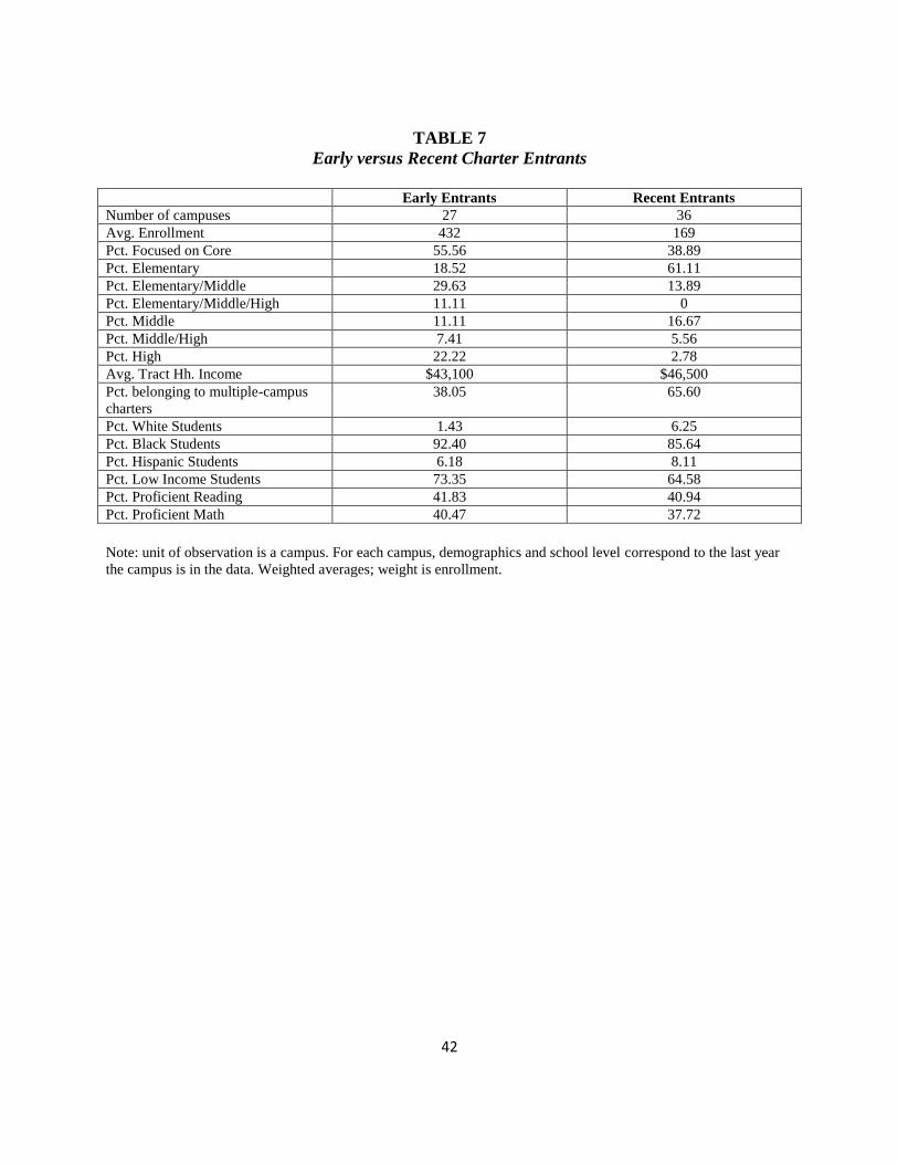
42

TABLE 7

Early versus Recent Charter Entrants

Early Entrants Recent Entrants

Number of campuses 27 36

Avg. Enrollment 432 169

Pct. Focused on Core 55.56 38.89

Pct. Elementary 18.52 61.11

Pct. Elementary/Middle 29.63 13.89

Pct. Elementary/Middle/High 11.11 0

Pct. Middle 11.11 16.67

Pct. Middle/High 7.41 5.56

Pct. High 22.22 2.78

Avg. Tract Hh. Income $43,100 $46,500

Pct. belonging to multiple-campus

charters

38.05 65.60

Pct. White Students 1.43 6.25

Pct. Black Students 92.40 85.64

Pct. Hispanic Students 6.18 8.11

Pct. Low Income Students 73.35 64.58

Pct. Proficient Reading 41.83 40.94

Pct. Proficient Math 40.47 37.72

Note: unit of observation is a campus. For each campus, demographics and school level correspond to the last year

the campus is in the data. Weighted averages; weight is enrollment.

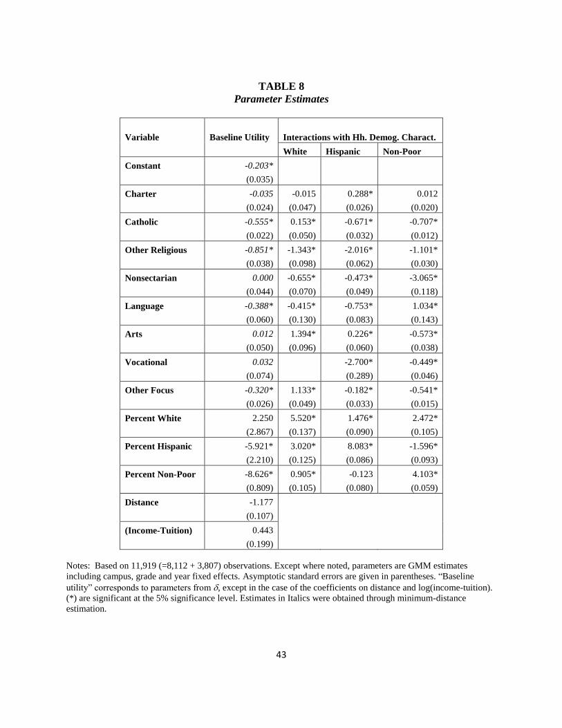
43

TABLE 8

Parameter Estimates

Variable Baseline Utility Interactions with Hh. Demog. Charact.

White Hispanic Non-Poor

Constant -0.203*

(0.035)

Charter -0.035 -0.015 0.288* 0.012

(0.024) (0.047) (0.026) (0.020)

Catholic -0.555* 0.153* -0.671* -0.707*

(0.022) (0.050) (0.032) (0.012)

Other Religious -0.851* -1.343* -2.016* -1.101*

(0.038) (0.098) (0.062) (0.030)

Nonsectarian 0.000 -0.655* -0.473* -3.065*

(0.044) (0.070) (0.049) (0.118)

Language -0.388* -0.415* -0.753* 1.034*

(0.060) (0.130) (0.083) (0.143)

Arts 0.012 1.394* 0.226* -0.573*

(0.050) (0.096) (0.060) (0.038)

Vocational 0.032 -2.700* -0.449*

(0.074) (0.289) (0.046)

Other Focus -0.320* 1.133* -0.182* -0.541*

(0.026) (0.049) (0.033) (0.015)

Percent White 2.250 5.520* 1.476* 2.472*

(2.867) (0.137) (0.090) (0.105)

Percent Hispanic -5.921* 3.020* 8.083* -1.596*

(2.210) (0.125) (0.086) (0.093)

Percent Non-Poor -8.626* 0.905* -0.123 4.103*

(0.809) (0.105) (0.080) (0.059)

Distance -1.177

(0.107)

(Income-Tuition) 0.443

(0.199)

Notes: Based on 11,919 (=8,112 + 3,807) observations. Except where noted, parameters are GMM estimates

including campus, grade and year fixed effects. Asymptotic standard errors are given in parentheses. “Baseline

utility” corresponds to parameters from , except in the case of the coefficients on distance and log(income-tuition).

(*) are significant at the 5% significance level. Estimates in Italics were obtained through minimum-distance

estimation.

44

FIGURE 1

Number of Public, Charter and Private School Campuses

FIGURE 2

Enrollment in Public, Charter and Private School Campuses

020

40

60

80

100

120

140

Num

ber

of C

am

puses

2003 2004 2005 2006 2007Year

Public Charter

Private

0

20,0

00

40,0

00

60,0

00

80,0

00

Num

ber

of S

tudents

2003 2004 2005 2006 2007Year

Public Charter

Private Total Enrollment

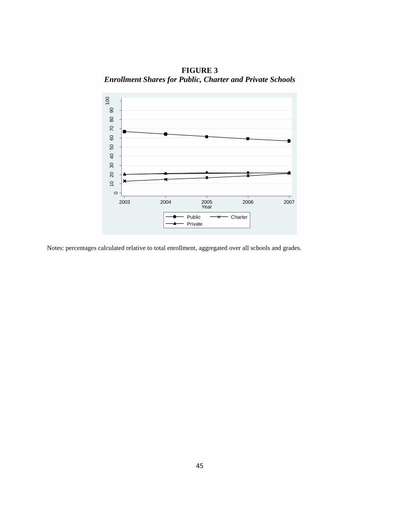
45

FIGURE 3

Enrollment Shares for Public, Charter and Private Schools

Notes: percentages calculated relative to total enrollment, aggregated over all schools and grades.

010

20

30

40

50

60

70

80

90

100

Enro

llment S

hare

(P

erc

ent)

2003 2004 2005 2006 2007Year

Public Charter

Private

46

FIGURE 4a

Geographic Location of Elementary Schools in DC in 2007

Note: Elementary schools include elementary, elementary/middle, and elementary/middle/high schools.

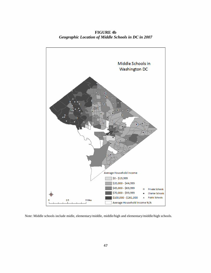
47

FIGURE 4b

Geographic Location of Middle Schools in DC in 2007

Note: Middle schools include midle, elementary/middle, middle/high and elementary/middle/high schools.

48

FIGURE 4c

Geographic Location of High Schools in DC in 2007

Note: High schools include high, middle/high, and elementary/middle/high schools.

49

FIGURE 5a - Public Schools: Aggregate Enrollment Share by Grade

FIGURE 5b - Charter Schools: Aggregate Enrollment Share by Grade

FIGURE 5c - Private Schools: Aggregate Enrollment Share by Grade

Note: Shares are calculated relative to the total enrollment per grade, where total = aggregate enrollment over public,

charter and private schools.

0.00%

20.00%

40.00%

60.00%

80.00%

K 1 2 3 4 5 6 7 8 9 101112

Pe

rce

nta

ge

Grade

2003

2004

2005

2006

2007

0.00%

10.00%

20.00%

30.00%

40.00%

K 1 2 3 4 5 6 7 8 9 101112

Pe

rce

nta

ge

Grade

2003

2004

2005

2006

2007

0%

5%

10%

15%

20%

25%

30%

35%

40%

K 1 2 3 4 5 6 7 8 9 10 11 12

Pe

rce

nta

ge

Grade

2003

2004

2005

2006

2007

50

FIGURE 6

Number of Public, Charter and Private Schools by Grade in 2003 and 2007

FIGURE 7

Average Grade Enrollment in Public, Private and Charter Schools in 2007

0

10

20

30

40

50

60

70

80

90

100

110

120

K 1 2 3 4 5 6 7 8 9 10 11 12

Grade

Charter 2003

Charter 2007

Public 2003

Public 2007

Private 2003

Private 2007

0

20

40

60

80

100

120

140

160

180

200

220

K 1 2 3 4 5 6 7 8 9 10 11 12

Grade

Charter 2007

Public 2007

Private 2007

1 Appendix I. School-Level Data

1.1 Public Schools

The starting point for this dataset was audited enrollments from the District of Columbia O¢ ce ofState Superintendent of Education (OSSE), available at http://osse.dc.gov. From here we obtainedthe list of public schools along with their grade-level enrollment.

Our list only includes regular schools. This means that relative to the original OSSE list, wealternative schools, special education schools, and early childhood centers.We excluded schools listedas alternative by the OSSE, schools that report their program as alternative in the Common Coreof Data (CCD), and schools listed as alternative during the corresponding years by DCPS. We alsoexcluded schools that o¤er residential programs, such as Ballou Stay and Spingarn Stay. In total, weeliminated 11 alternative schools from the original OSSE lists. We excluded schools listed as specialed by OSSE and schools that report their type as special ed in the CCD. Some schools report theirtype as special ed only during one or two years during our sample period, in which case we calledthe individual schools to gauge their type and removed them from the data if they were special ed.In total, we eliminated 22 special ed schools from the original OSSE lists. Early childhood centersinclude one or several of the following: pre-school, pre-kindergarten, and kindergarten, and do notinclude regular grades. We excluded early childhood centers as long as they never had enrollment inregular grades (1 through 12) during the sample period. For instance, if an early childhood centeradded �rst grade in 07, then the school was included for all 5 years.

Below is the list of information and sources for each school, along with the construction ofthe corresponding variables:

� Address: geographic address of the school. The main source for this variable was the CCD.When the address was not consistent over time, we used Google Earth and Google Maps tosee whether the di¤erent addresses corresponded to the same geographic location or not. Ifnot, we consulted the school�s web site, or called the school to track down the history of itslocation. In the absence of other information, we used the most recently reported address. Wegeocoded all addresses.

� School enrollment: total school enrollment, excluding ungraded and adult students. Source:own calculations based on OSSE.

� Grade-level enrollment (grades preschool through 12). Source: OSSE.

� Focus: the school�s curricular focus. Source: Filardo et al (2008).

� Percent of white students: percent of White students in the school. Source: own cal-culations based on CCD. For the few cases in which the CCD data was not available, weused the demographics reported to ful�ll No Child Left Behind (NCLB) requirements (seehttp://www.nclb.osse.dc.gov/). Note, however, that the NCLB requirements pertain to thestudents enrolled in the grades tested for the sake of NCLB accountability, not to the entirestudent body. When using the NCLB web site, we computed percent of white students asthe ratio between the number of white students in the grades tested and the total number ofstudents in those grades.

� Percent of black students, percent of Hispanic students, percent of students ofother ethnicities: constructed similarly to percent of white students.

� Percent of low income students: calculated as the percent of students who receive free orreduced lunch. Source: own calculations based on CCD. For the few cases in which the CCDdata was not available we used the demographics reported in ful�llment of NCLB requirements.

51

� Reading pro�ciency: percent of students who are pro�cient in Reading.Source: http://www.nclb.osse.dc.gov/. In 03 and 04, pro�ciency levels were determined ac-cording to the Stanford-9 assessment. To be considered pro�cient, a student was supposed toscore at the national 40th percentile or higher. Since 05, pro�ciency has been determined ac-cording to DC CAS (Comprehensive Assessment System). See http://www.nclb.osse.dc.gov/faq.aspfor more information.

� Prior to 05, the grades tested were 3, 5, 8 and 10 (according to the School Performance Reportsfor PCBS-authorized charter schools, and according to our own calculations comparing grade-level enrollment with number of students tested). Since 05, the grades tested have been 3, 4, 5,6, 7, 8 and 10 (according to http://www.nclb.osse.dc.gov/aboutayp.asp, School PerformanceReports and our own calculations comparing grade-level enrollment with number of studentstested).

� The achievement website, http://www.nclb.osse.dc.gov/faq.asp , reports pro�ciency for ele-mentary and secondary schools. According to http://www.nclb.osse.dc.gov/faq.asp, schoolsare classi�ed as elementary or secondary as follows. Since 05, elementary schools are schoolswith a 3rd and/or 5th grade. If the school goes above the 6th grade it must also have a 3rdgrade. Secondary schools are schools with no 3rd and a grade above 6th. Prior to 2006, schoolswith a wide grade range were required to meet both the elementary and secondary targets.The general rule for most schools was that they were classi�ed as elementary if they had nograde above 6 and as secondary if they had no grade below 5. Schools that did not meet eitherof these criteria had to meet the targets at both levels.

� For some schools and years, pro�ciency data are not available for one of the following threereasons: 1) the school only includes early childhood enrollment; 2) the school only includesgrades that are not tested (for instance, the school includes kindergarten and �rst grade only);3) the school includes grades that are tested, but enrollment in those grades is below theminimum threshold for reporting requirements. The last reason is the most prevalent cause ofmissing pro�ciency. See below for the imputations made in those cases.

� Math pro�ciency: percent of students who are pro�cient in Math. Constructed similarly asreading pro�ciency.

� Year of Opening: year the school opened if it was not open in 03. Using the CCD �status�variable and web searches we veri�ed the school�s initial year, which is the �rst year for whichwe have records.

� Year of Closing: year the school closed if it was not open in 07. The variable stores the �rstyear that the school was no longer open. We veri�ed the content of this variable using theCCD �status�variable and web searches.

� Year of Merge: year the school merged with another school. The variable stores the �rstyear that the school no longer operates separately, which is the �rst year for which we havejoint records.

Ethnic composition and low-income status of the student body were missing for 2 and 4(out of 701) observations respectively; these were schools with very low enrollment. To the cases ofmissing ethnic composition we imputed the school�s average ethnic composition over the years forwhich we do have data. When possible, we imputed the predicted value coming from a school-speci�clinear trend.

52

Achievement was missing in 16 out of 701 observations. To these observations, we imputedthe predicted achievement coming from the regression of school-level pro�ciency rates on year dum-mies, ethnic composition variables, percent of low income students, enrollment, and school �xede¤ects. In cases in which we had no pro�ciency data for the school at all, we ran a similar regres-sion excluding school �xed e¤ects and including dummies for school level, and used the resultingpredicted values for our imputations.

1.2 Charter Schools

As with public schools, the starting point for this dataset was audited enrollments from the Districtof Columbia O¢ ce of State Superintendent of Education (OSSE), available at http://osse.dc.gov.From here we obtained the list of public schools along with their enrollment for preschool, pre-kindergarten, kindergarten, each grade between 1 and 12, and enrollment of ungraded and adultstudents.

For consistency with public schools, we excluded alternative schools. We identi�ed alterna-tive schools based on OSSE�s classi�cation, the schools�mission statements, and the self-reportedprogram type in the CCD. We excluded schools in which ungraded or adult students constitute themajority of the student body, and schools with residential programs.

By law, charter schools cannot serve special education students exclusively. However, theycan o¤er services targeted to speci�c populations even though their enrollment must be open to allstudents. Only one charter school in D.C., St. Coletta, serves special ed students exclusively, andwas approved to that end by the Board of Education (BOE) when it was chartered. We excludedschools whose services target mostly special ed students. We identi�ed those schools based onOSSE�s classi�cation, the schools�mission statements, the self-reported program type in the CCD,and phone conversations with sta¤ from the Public Charter School Board (PCSB).

We excluded early childhood schools only if they never added regular grades. We alsoexcluded online campuses.

Some non-early childhood charters opened an early childhood campus during the sampleperiod. We only included these campuses if at some point they added regular grades. CommunityAcademy-Amos II is an early childhood campus that did not include regular grades (at least notduring our sample period) and is hence not included in our data. Similarly, Roots Academy openedan early childhood campus in 07, which we did not include in the data. KIPP-LEAP is an earlychildhood campus that opened in 07 and is not included either. In contrast, E.L. Haynes opened acampus in 07 for early childhood and �rst grade; this campus is included in our data.

Below is the list of variables for charter schools:

� Address: geographic location of the campus. For PCSB schools, the main source was theSPRs. For BOE schools, the main source was the CCD. We supplemented these sources withweb and Internet archive searches, and phone calls to the individual schools. We geocoded alladdresses.

� Several schools moved in the middle of the school year, temporarily relocated, or closed. Weconsulted the SPRs and various web sites to handle these cases. If the school moved in themiddle of a school year, the address variable contains the more recent address. Some schoolsrelocated some students for a few months during renovations. Since this was a temporaryarrangement and parents knew it, we did not consider this a change in address.

� Statement: the school�s mission statement. Source: schools�web sites, FOCUS, SPRs.

� Focus: the school�s curricular focus. Source: school statements, and Filardo et al (2008).

53

� School enrollment: total school enrollment, excluding ungraded and adult students. Source:own calculations based on OSSE.

� Grade-level enrollment (grades preschool through 12). Source: OSSE.

� Percent of white students: percent of White students in the school. For PCSBcharters, the source is the School Performance Reports (SPRs) when available. Only for onecampus and year (Tri Community in 07), does the SPR not include demographic information,in which case we use the NCLB data from http://www.nclb.osse.dc.gov/ otherwise.

� For BOE charters in 2007, the source is the SPRs (in 2007, the PCSB began including theBOE-authorized charters in its reports). For BOE charters before 2007, the source is theNCLB web site. Note that the NCLB information pertains only to students in grades tested,not to the whole student body of a school. These sources were supplemented by the CCDwhen needed. When the school has multiple campuses but we only have one set of ethniccomposition data, we impute it to all campuses.

� Percent of black students, percent of Hispanic students, percent of students ofother ethnicities: constructed similarly to percent of white students.

� Percent of low income students: fraction of students on free or reduced lunch. For PCSBcharters, the source is the SPRs. For BOE charters, the source is NCLB information inhttp://www.nclb.osse.dc.gov/. These sources were supplemented by the CCD when neededand possible. When the school has multiple campuses but we only have one set of low-incomevariables, we impute it to all campuses.

� Reading pro�ciency: percent of students who are pro�cient in Reading. See public schoolsfor sources and construction. Some charters span elementary and secondary grades, and thisa¤ected their reporting. For instance, Capital City had to meet elementary and secondarytargets before 05, and for those years it reported two sets of scores. Since 05, Capital Cityhas had to meet only one target, has been considered an elementary school for the sake ofreporting, and has had to report only one set of scores. In general, when the school had onlyone campus but separate pro�ciencies for elementary and secondary students, we combinedthem into a single pro�ciency indicator for comparability with other years in which we had asingle pro�ciency indicator. For multi-campus charters we usually had achievement data foreach campus. When we did not, we imputed the available data to all the campuses.

� As with public schools, we did not have pro�ciency data for some campus and years for thereasons enumerated above. In the case of many PCSB schools for which the NCLB web sitedid not report test scores due to low enrollment, we obtained pro�ciency rates from the SPRs.This was not possible for BOE schools with low enrollment since the SPRs only cover PCSBschools before 07. In cases in which we could not �nd pro�ciency data, we made imputations(see below).

� Math pro�ciency: percent of students who are pro�cient in Math. Constructed similarly asreading pro�ciency.

� Year of Opening: year the campus opened. Source: SPRs, FOCUS, web searches. Thevariable stores the �rst Fall that the school is open.

� Year of Closing: year the school closed, even if it closed after 07. The variable storesthe �rst year that the school is no longer open. The sources are Center for Education Reform(http://www.edreform.com/accountability/charters/CER_ClosedCharterSchools2009.pdf), cur-rent SPRs and PCSB listings of charter schools, current NCLB reports, and web searches.

54

� Note that Washington Academy was taken over by Howard Road in Spring 08 � i.e., in themiddle of school year 07. Hence, the year of closing is 2007 for Washington Academy becauseit the �rst year for which Washington Academy no longer exists. In fact, for the school year07/08, data were reported by Howard Road, and the SPRs report data for Howard Roadcampuses noting that they were former campuses of Washington Academy. We chose not toadd campuses to Howard Road for 07 because the campuses did not physically move �theysimply changed ownership.

� Reason for Closing: reason for closing (academic / �nancial / mismanagement). Source:Center for Education Reform, SPRs, web searches.

Percent of low-income students was missing for 9 out of 230 observations respectively. Theseschools had low enrollments. To most of these cases we imputed the school�s average percent of low-income students, the average being calculated over the years for which the school does have data.

In the case of missing pro�ciency rates (36 out of 230 observations), we made imputationssimilar to those described for public schools, the only di¤erence being that we used school-�xede¤ects (as opposed to campus-�xed e¤ects) in the predicting regressions.

1.3 Private Schools

The starting point for this dataset was the list of private schools from the Private School Survey(PSS). Since the PSS is biennial, we included the 2003, 2005 and 2007 waves in our data.

PSS classi�es schools as regular, vocational, special ed, and other/alternative. 92 percent ofthe schools in our dataset are regular, and the remaining schools are classi�ed as other/alternative.Although an alternative public school is usually a school for students with behavioral problems, analternative private school is often a school that o¤ers a specialized rather than a regular curriculum.In these cases, we kept alternative schools. We eliminated vocational schools because they enrolledexclusively ungraded students. We also eliminated special ed schools, early childhood centers (aslong as they never had enrollment in regular grades during the sample period), and schools thatonly teach ungraded students. Most of the schools we eliminated are early childhood centers.

Since 2004 was not included in PSS, we assigned 2004 values to the variables through linearinterpolation of 2003 and 2005, and similarly for 2006. For instance, we calculated the percent ofWhite students for a school in 2004 as the average of percent white in 2003 and 2005.

Some schools did not report to the survey for some waves. For instance, Edmund Burkehas data for 2001, 2005 and 2007 but not for 2003, which means that we need to make some dataimputations for 2003, 2004 and 2006. The imputed data for 2003 is the average between 2001 and2005. Treating the imputed 2003 as actual data, we then imputed data for 2004 as the averagebetween 2003 and 2004.

If a school does not appear again in PSS after a particular wave, we assumed that the lastyear of operation was the year of the last wave in our data. Similarly, if a school appears in aparticular wave but not in any of the following waves, we assume that its last year is the year of thelast wave for which we have data.

Below is the list of information and sources for each campus, along with the construction ofthe corresponding variables:

� Address: geographic location of the campus. We supplemented PSS with web and Internetarchive searches, and phone calls to the individual schools. We geocoded all addresses.

� Type: Catholic, other religious or non-sectarian. Source: PSS.

55

� School enrollment: total school enrollment, excluding ungraded and adult students. Source:own calculations based on PSS.

� Grade-level enrollment: number of students in each grade between K and 12.

� Percent of white students: percent of White students in the school. Source: own calcu-lations based on the reported number of White students and the total enrolment. Since thenumber of students for each ethnicity spans grades K through 12, we used K-12 enrollment aswell in the denominator.

� Percent of black students, percent of Hispanic students, percent of students ofother ethnicities: constructed similarly to percent of white students.

� Percent of low income students: since PSS does not collect this information, we imputedit based on a logistic regression for public and charter schools of percent low income on schoolethnic composition, enrollment, and average household income of the school�s tract. As acheck, we compared the resulting predictions with data from OSSE on the percent of studentsreceiving free and reduced lunch in private schools. Our predictions compare favorably withthe OSSE data.

� Tuition: annual tuition by grade for the 2010/11 school year. Source: web searches. Whentuition information was not available, we imputed tuition based on the predicted values arisingfrom the regression of tuition on grade, school type (based on the nine-type private schoolclassi�cation used by PSS), average household income of the tract where the school is located,school enrollment, and a quadratic term in school enrollment. Both observed and predictedtuitions are expressed in dollars of 2000.

2 Appendix II. Pro�ciency Rate Regression

As described in the paper (eq. (6)), student i�s achievement in school j, grade g and time (the vari-able Aijgt) is a function of school time-invariant characteristics yj , student body �Djt, the student�sown characteristics Di, and the student-school interaction yjDi. We assume that the probabilityqijgt that i passes the pro�ciency test is monotonically related to her achievement, and is given bythe following speci�cation:

qijgt = yj�q + �Djt�

q +Di!q + yjDi~�

q+ �qjgt + v

qijgt; (1)

where vqijgt is a zero-mean idiosyncratic shock. A student who passes is deemed "pro�cient".The school-level expected share of pro�cient students is

qjt =

Pg2�jt

Pi2Ijgt qijgt

jIjtj;

where Ijt is the set of students enrolled in school j at year t. Averaging qijgt over students andgrades we obtain the following:

qjt = yj�q + �Djt�

q + yj �Djt~�q+ �qjt; (2)

where the identity �Djt =

Pg2�jt

Pi2Ijgt

Di

jIjgtj is applied. The following new variables are introduced:

�q = �q + !q and �qjt =P

g2�jt

Pi2Ijgt

(�qjgt+vqijgt)

jIjtj :1

1This averaging is possible because the probability of passing the test is speci�ed as a linear function.

56

In (2), we decompose shock �qjt as follows

�qjt = �qj + �

qt +��

qjt:

Substituting the above expression into (2) we obtain the following expression for the expected shareof pro�cient students:

qjt = yj�q + �Djt�

q + yj �Djt~�q+ �qj + �

qt +��

qjt: (3)

Let �qjt be the observed pro�ciency rates. They are related to the expected pro�ciency ratesin the following way:

�qjt = yj�q + �Djt�

q + yj �Djt!q + �qj + �

qt +��

qjt + v

qjt (4)

where vqjt = �qjt � qjt incorporates sampling and measurement error and is conditionally meanindependent of all the explanatory variables in (4). However, it is possible that ��qjt is correlatedwith ��jgt, and as consequency that �Djt is correlated with ��

qjt. Hence, we use IV estimation for

(4).

3 Appendix III. Market Size and Outside Good

In this appendix we �rst describe the estimation of the joint distribution of household location, childage and race, parental income and child poverty status for year 2000 and the adjustments neededfor years 2003-2007. Then we describe the construction of choice sets for households in di¤erentlocations.

In what follows we use the term �demographic type� to refer to a combination of race(Black, White and Hispanic), income (16 values for income, each one representing the midpoint ofthe corresponding Census income bracket), and poverty status (eligible for free- or reduced-lunch,and not eligible). This yields a total of 96 demographic types. Our goal is to estimate the numberof children in each of these types for each of the 13 grades and 433 locations in our data.

Since each grade is a market, calculating market size amounts to determining the numberof children who are eligible for each grade in Washington, D.C. in each year between 2003 and 2007.Given our data on aggregate enrollment by grade and year, the share of the outside good for a givengrade and year is equal to (market size �aggregate enrollment) / market size.

The main di¢ culty in calculating market size is that we do not have direct information onthe number of children eligible for each grade in each year. In the absence of this information, themere count of children by age and year would be helpful, but we do not have this information either.Instead, to calculate market size we rely on the following pieces of data:

1. The 2000 count of children by age (see Table A1);

2. The intercensal estimates of the number of children 5-13 and 14-17 year old brackets (see TableA2);

3. The 2000 count of enrolled and not enrolled children, and the resulting percent of children whoare not enrolled. The latter is our best proxy for the outside good share for year 2000;

4. Observed enrollment for each grade and year (see Table A4).

57

To estimate the number of children by age in each year, one could apply the annual ratesof growth implied by Table A2 to the 2000 observed number of children in each age (see Table A1).Since these rates of growth di¤er by age groups, one could apply to each age the rate that correspondsto its age group. In principle, the resulting number of children per age should be at least as large asthe observed enrollment in the corresponding grades (see Table A4). When we apply this procedure,for grades 4-8 we estimate a number of children (or potential enrollment) that is lower than theactual enrollment, thus implying a negative share of the outside good. One possible explanation isthe existence of di¤erent growth rates within the age group 5-13. For instance, children who are5-13 years old in 2003 would have been 2-10 years old in 2000. As Table 1 shows, there is a fairamount of variation in the number of children in each age between 2 and 10. Thus, it is plausiblethat each individual age would grow at a di¤erent annual rate. Another possible explanation is theexistence of complex patterns of grade retention.

Since we do not have data to disentangle these possibilities, after evaluating a number ofsolutions we opted for in�ating the observed enrollment for each grade g and year t by a factor #gtin order to calculate potential enrollment by grade. These factors are chosen so that their impliedoutside good shares by age match up with 2000 Census outside good shares (see Table A3) We optedfor this solution not only because it was simple, but also because our most direct evidence on theoutside good share comes from the 2000 Census. Thus, we calculate market size for (g; t) as observedaggregate enrollment for (g; t) � #gt. For computational reasons we imposed the constraint that theresulting outside share by grade should be greater than or equal to 0.01.

For the calculation of our adjustment factor, we modi�ed the 2000 Census outside goodshares slightly to accommodate some features of our data. In particular, our enrollment data isbased on regular schools (thus excluding special ed or alternative schools, which are more prevalentin middle or high school than elementary school), and excludes schools that are specialized in earlychildhood (i.e., that do not include grades above kindergarten). Thus, we used an outside goodshare of 3% for grades K through 8 (corresponding to ages 5-14 in the 2000 Census) and 10% forgrades 9 through 12 (corresponding to ages 14-17 in the Census).

Our solution has the appealing feature of delivering an estimated number of children whoseannual growth rate is consistent with the growth rates implied by the intercensal Census estimates(see Table A2). In particular, potential enrollment given our solution grows at the following ratesbetween 2003 and 2007: -13% for grades K through 8, and 7% for grades 9 through 12. These ratesline up with the Census growth rates for the corresponding age groups (equal to -13% and 13%,respectively) for the same period.

4 Appendix IV. Household Characteristics and Choice Sets

In this appendix we �rst describe the estimation of the joint distribution of household location, childage and race, parental income and child poverty status for year 2000 and the adjustments neededfor years 2003-2007. Then we describe the construction of choice sets for households in di¤erentlocations.

In what follows we use the term �demographic type� to refer to a combination of race(Black, White and Hispanic), income (16 values for income, each one representing the midpoint ofthe corresponding Census income bracket), and poverty status (eligible for free- or reduced-lunch,and not eligible). This yields a total of 96 demographic types. Our goal is to estimate the numberof children in each of these types for each of the 13 grades and 433 locations in our data.

58

4.1 Household Types for Year 2000

The main challenge in measuring the number of households in each (grade, demographic type)combination at the block group level is the fact that we do not observe the joint distribution ofchild age, race, household income and poverty status at the block group level. Instead, the Censusprovides us with the following information:

� tract-level joint distribution of age and race;

� tract-level joint distribution of age bracket, race and poverty status2 ;

� tract-level joint distribution of family income (by brackets) and race;

� block group-level joint distribution of age brackets and race.

Thus, we use this information to calculate the number of households in each demographictype, for each grade and location. Recall that Washington, D.C. includes 433 block groups and 188Census tracts. The calculations described below apply to the 185 tracts that do have children aged5-18 and the corresponding block groups. We proceeded as follows:

1. Note that for each block group we observe the joint distribution of age brackets and race, andat the tract level we observe the joint distribution of individual ages and race. We assumethat for a given age bracket and race, the distribution of individual ages is the same for allthe block groups that belong to a tract. Hence, for each block group, age bracket and race weimputed the distribution of individual ages of the corresponding tract and race.

2. For each tract we observe the joint distribution of age brackets, race and poverty status. Weassume that for a given tract, the distribution of race and poverty status is the same for allindividual ages within a given age bracket. We also assume that the joint distribution of age,race, and poverty status is the same for all the block groups located within a given tract.Hence, for each block group, individual age and race, we imputed the poverty distribution ofthe corresponding tract.

3. Based on steps (1) and (2), we calculated the number of children in each (age, race, povertystatus) combination in each block group. For a given block group, denote this number as narp,where a=age; r=race; p=poverty status.

4. The tract-level income distribution for families is not adjusted by family size and hence doesnot re�ect income per child. In the absence of data on the joint distribution of family incomeand size, we calculated tract-level average family income and size by race and constructed thecity-level joint distribution of average family income and size. Then we reweighted the originaltract-level family income distribution to re�ect di¤erences in family size by income bracket.

2Federal guidelines (see http://www.fns.usda.gov/cnd/governance/notices/iegs/iegs.htm) establish eligibility forfree- or reduced-price lunch based on household size and income. To qualify for free (reduced) lunch, a child mustlive in a household whose income is below 130 (185) percent of the Federal poverty guidelines for that householdsize. We pool children eligible either for free or reduced lunch into a single category. Since the Census reports thenumber of children in each age bracket and race whose household income falls below 130%, or between 130% and 185%percent of the poverty guideline given their household size, we can calculate the number of children eligible for free-or reduced-lunch as the total number of children whose household income falls below 185% of the poverty guideline.Thus, �poverty status� is a binary variable that describes whether the child is eligible for free- or reduced-lunch ornot. In some parts of the paper, we use �low-income� to describe a child who is eligible for free- or reduced lunch.

59

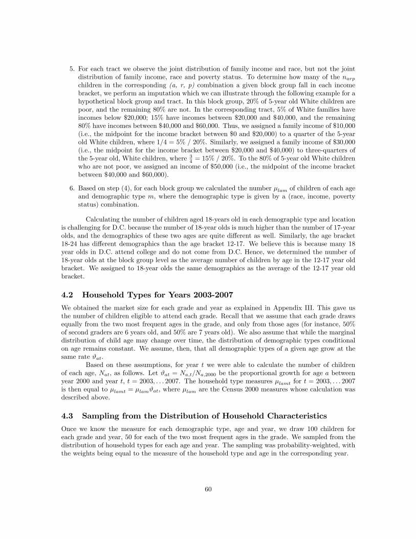
5. For each tract we observe the joint distribution of family income and race, but not the jointdistribution of family income, race and poverty status. To determine how many of the narpchildren in the corresponding (a, r, p) combination a given block group fall in each incomebracket, we perform an imputation which we can illustrate through the following example for ahypothetical block group and tract. In this block group, 20% of 5-year old White children arepoor, and the remaining 80% are not. In the corresponding tract, 5% of White families haveincomes below $20,000; 15% have incomes between $20,000 and $40,000, and the remaining80% have incomes between $40,000 and $60,000. Thus, we assigned a family income of $10,000(i.e., the midpoint for the income bracket between $0 and $20,000) to a quarter of the 5-yearold White children, where 1/4 = 5% / 20%. Similarly, we assigned a family income of $30,000(i.e., the midpoint for the income bracket between $20,000 and $40,000) to three-quarters ofthe 5-year old, White children, where 34 = 15% / 20%. To the 80% of 5-year old White childrenwho are not poor, we assigned an income of $50,000 (i.e., the midpoint of the income bracketbetween $40,000 and $60,000).

6. Based on step (4), for each block group we calculated the number �lam of children of each ageand demographic type m, where the demographic type is given by a (race, income, povertystatus) combination.

Calculating the number of children aged 18-years old in each demographic type and locationis challenging for D.C. because the number of 18-year olds is much higher than the number of 17-yearolds, and the demographics of these two ages are quite di¤erent as well. Similarly, the age bracket18-24 has di¤erent demographics than the age bracket 12-17. We believe this is because many 18year olds in D.C. attend college and do not come from D.C. Hence, we determined the number of18-year olds at the block group level as the average number of children by age in the 12-17 year oldbracket. We assigned to 18-year olds the same demographics as the average of the 12-17 year oldbracket.

4.2 Household Types for Years 2003-2007

We obtained the market size for each grade and year as explained in Appendix III. This gave usthe number of children eligible to attend each grade. Recall that we assume that each grade drawsequally from the two most frequent ages in the grade, and only from those ages (for instance, 50%of second graders are 6 years old, and 50% are 7 years old). We also assume that while the marginaldistribution of child age may change over time, the distribution of demographic types conditionalon age remains constant. We assume, then, that all demographic types of a given age grow at thesame rate #at.

Based on these assumptions, for year t we were able to calculate the number of childrenof each age, Nat, as follows. Let #at = Na;t=Na;2000 be the proportional growth for age a betweenyear 2000 and year t, t = 2003; : : : 2007. The household type measures �lamt for t = 2003; : : : 2007is then equal to �lamt = �lam#at, where �lam are the Census 2000 measures whose calculation wasdescribed above.

4.3 Sampling from the Distribution of Household Characteristics

Once we know the measure for each demographic type, age and year, we draw 100 children foreach grade and year, 50 for each of the two most frequent ages in the grade. We sampled from thedistribution of household types for each age and year. The sampling was probability-weighted, withthe weights being equal to the measure of the household type and age in the corresponding year.

60

4.4 School Choice Sets

To determine the set of schools that are eligible to a household based on her location, the critical issueis determining the public school associated to each block group for each grade and year. To arriveat this association, we �rst associated block groups with attendance zones, and then attendancezones with schools. We have a set of associations for 2003 and 2004 (prior to the attendance zoneboundary changes), and another for 2005-2007. We refer to these as the 2003 and 2005 associations,respectively. The associations were done using GIS software.

While the task was relatively straightforward for 2005, it was not so for 2003. For instance,in 2003 some attendance zones contain no schools, while others contain two; some attendance zonescontain a school within their physical boundary that does not have the same name as the attendancezone; etc. To �x these problems, we de�ned a �main�and a �secondary� school when needed foreach attendance zone and school level. For a given attendance zone, the main school is the schoolwhose name matches the attendance zone�s, or the school that lies within the physical boundariesof the school and does not have the same name as the attendance zone, but does not have anotherattendance zone named after the school. The additional school (when it exists) is the school thatdoes not have a speci�c attendance zone associated to it and lies within a zone that does have amain school. Overall, additional schools are quite rare in the data.

We determined main and additional schools based on conversations with GIS experts fromDCPS. Those conversations also provided a solution to the problem that the attendance zones�mapcontains holes � i.e., some block groups are not associated to any attendance zone. We assignedthose block groups to the closest public school for each level.

61

62

TABLE A1

Number of children by age

Age Number

0 6306

1 6123

2 6352

3 6332

4 6657

5 6692

6 6985

7 7095

8 7068

9 7069

10 6887

11 6039

12 5674

13 5636

14 5426

15 5469

16 5578

17 5787

18 5595

Note: data from the 2000 Census. For each age, the count is an aggregate over Census tracts. For the count of 18-year

olds, see Appendix IV.

TABLE A2

Number of Children by Age Bracket

2000 2003 2004 2005 2006 2007

% Change

07 w.r.t 03

Total Population 571,744 577,777 579,796 582,049 583,978 586,409 1.49%

Children Below 5 yrs. 32,404 33,357 34,167 34,771 34,677 35,794 7.31%

Elem. Sch. Age Children (5-13) 59,746 59,561 57,186 55,078 53,873 52,068 -12.58%

High Sch.-Age Children (14-17) 22,504 23,145 24,534 25,156 26,049 26,198 13.19%

Note: for 2000, counts are from the 2000 Census. For the other years, counts are from Census Bureau estimates.

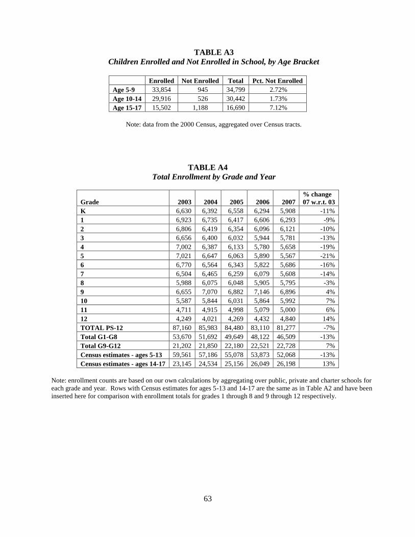
63

TABLE A3

Children Enrolled and Not Enrolled in School, by Age Bracket

Enrolled Not Enrolled Total Pct. Not Enrolled

Age 5-9 33,854 945 34,799 2.72%

Age 10-14 29,916 526 30,442 1.73%

Age 15-17 15,502 1,188 16,690 7.12%

Note: data from the 2000 Census, aggregated over Census tracts.

TABLE A4

Total Enrollment by Grade and Year

Grade 2003 2004 2005 2006 2007

% change

07 w.r.t. 03

K 6,630 6,392 6,558 6,294 5,908 -11%

1 6,923 6,735 6,417 6,606 6,293 -9%

2 6,806 6,419 6,354 6,096 6,121 -10%

3 6,656 6,400 6,032 5,944 5,781 -13%

4 7,002 6,387 6,133 5,780 5,658 -19%

5 7,021 6,647 6,063 5,890 5,567 -21%

6 6,770 6,564 6,343 5,822 5,686 -16%

7 6,504 6,465 6,259 6,079 5,608 -14%

8 5,988 6,075 6,048 5,905 5,795 -3%

9 6,655 7,070 6,882 7,146 6,896 4%

10 5,587 5,844 6,031 5,864 5,992 7%

11 4,711 4,915 4,998 5,079 5,000 6%

12 4,249 4,021 4,269 4,432 4,840 14%

TOTAL PS-12 87,160 85,983 84,480 83,110 81,277 -7%

Total G1-G8 53,670 51,692 49,649 48,122 46,509 -13%

Total G9-G12 21,202 21,850 22,180 22,521 22,728 7%

Census estimates - ages 5-13 59,561 57,186 55,078 53,873 52,068 -13%

Census estimates - ages 14-17 23,145 24,534 25,156 26,049 26,198 13%

Note: enrollment counts are based on our own calculations by aggregating over public, private and charter schools for

each grade and year. Rows with Census estimates for ages 5-13 and 14-17 are the same as in Table A2 and have been

inserted here for comparison with enrollment totals for grades 1 through 8 and 9 through 12 respectively.