Did the 65 mph Speed Limit Save Lives?

Charles LavePatrick Elias

Reprint

UCTC No. 69

The University of CaliforniaTransportation Center

University of CaliforniaBerkeley, CA 94720

The University of CaliforniaTransportation Center

The University of California

Transportation Center (UCTC)is one of ten regional units

mandated by Congress andestablished in Fall 1988 tosupport research, education,and training in surface trans-portation. The UC Centerserves federal Region IX andis supported by matchinggrants from the U.S. Depart-

ment of Transportation, theCalifornia Department ofTransportation (Caltrans), andthe University.

Based on the Berkeley

Campus, UCTC draws uponexisting capabilities andresources of the Institutes ofTransportation Studies atBerkeley, Davis, Irvine, andLos Angeles; the Institute of

Urban and Regional Develop-ment at Berkeley; and severalacademic departments at theBerkeley, Davis, Irvine, andLos Angeles campuses.Faculty and students on other

University of Californiacampuses may participate in

Center activities. Researchersat other universities within theregion also have opportunitiesto collaborate with UC faculty

on selected studies.

UCTC’s educational andresearch programs are focused

on strategic planning forimproving metropolitanaccessibility, with emphasison the special conditions inRegion IX. Particular attentionis directed to strategies for

using transportation as aninstrument of economicdevelopment, while also ac-commodating to the region’spersistent expansion andwhile maintaining and enhanc-

ing the quality of life there.

The Center distributes reportson its research in workingpapers, monographs, and inreprints of published articles.It also publishes Access, amagazine presenting sum-

maries of selected studies. Fora list of publications in print,write to the address below.

University of CaliforniaTransportation Center

108 Naval Architecture BuildingBerkeley, California 94720Tel: 510/643-7378FAX: 510/643-5456

The contents of this report reflect the views of the author who is responsiblefor the facts and accuracy of the data presented herein. The contents do notnecessarily reflect the official views or policies of the State of California or theU.S. Department of Transportation. This report does not constitute a standard,specification, or regulation.

Did the 65 mph Speed Limit Save Lives?

Chades LavePatrick Elias

Department of EconomicsUniversity of California at Irvine

lrvine, CA 92717

Reprinted fromAccident Analysis and Prevention

Vol. 26, No. 1 (1994), pp. 49-62

UCTC No. 69

The University of California Transportation CenterUniversity of California at Berkeley

Accid. Anal. and Prey. Vol. 26, No. I, pp. 49-62, 1994Printed in the U.S.A. © 1993 Pergamon Press Ltd.

DID THE 65 MPH SPEED LIMIT SAVE LIVES’?.

CHARLES LAVE and PATRICK ELIAS

Department of Economics, University of California, Irvine, CA 92717, U.S.A.

(Received 19 August 1992; in revised form 15 April 1993)

Abstract--In 1987, most states raised the speed limit from 55 to 65 mph on portions of their rural interstatehighways. There was intense debate about the increase, and numerous evaluations were conducted afterwards.These evaluations share a common problem: they only measure the local effects of the change. But thechange must be judged by its system-wide effects. In particular, the new 65 mph limit allowed the statehighway patrols to shift their resources from speed enforcement on the interstates to other safety activitiesand other highways--a shift many highway patrol chiefs had argued for. If the chiefs were correct, the newallocation of patrol resources should lead to a reduction in statewide fatality rates. Similarly, the chance todrive faster on the interstates should attract drivers away from other, more dangerous roads, again generatingsystem-wide consequences. This study measures these changes and obtains surprising results. We find thatthe 65 mph limit reduced statewide fatality rates by 3.4% to 5.1%, holding constant the effects of long-termtrend, driving exposure, seat belt laws, and economic factors.

I. INTRODUCTION

In 1987, amid widespread controversy, 40 statesraised the speed limit to 65 mph on sections of theirrural interstate roads. Anticipation of the conse-quences varied widely: some predicted carnage, oth-ers said fatalities would decline. As might be ex-pected, there have been numerous studies of thenew speed limit. (See, for example: Baum, Wells,and Lund 1990; NHTSA 1989; Gallagher et al.1989.)

Most of these studies looked at the number offatalities, before and after the increase to 65 mph.The number usually increased since traffic usuallyincreased--but we should be looking at rates, i.e.fatalities per vehicle mile traveled (VMT). And allthe studies have confined themselves to looking atlocal effects: did raising the speed limit on highwayX affect fatalities on that highway?

But there are theoretical reasons to believe thatthe effect of the 65 mph limit will be felt across theentire highway system: (i) enforcing the 55 mph limiton the interstate highways required a substantialamount of highway patrol resources: the new 65 mphlimit allows highway patrols to shift these resourcesto other safety activities and other highways--some-thing they wished to do; (ii) the new 65 mph limitmight produce a shift of traffic from rural roads torural interstates; (iii) higher speeds on the rural inter-states might have psychological "spill-overs" thatencourage faster driving on other roads. Thus,changing the speed limit on the rural interstates is

likely to have consequences for other highways, sowe should take account of these broader effects.

This study analyzes the statewide conse-quences of raising the speed limit, treating highwaysand enforcement as a total system. We find that the65 mph speed limit reduced the statewide fatalityrate by 3.4%-5.1%, compared to those states thatdid not raise their speed limit.

II. THEORY: POLICE ENFORCEMENTAND TRAFFIC BEHAVIOR

AS A SYSTEM

Highway patrol resources are limited. If moreofficers are assigned to enforce speed limits on ruralinterstate highways, fewer can be assigned to othersafety activities such as truck safety inspections ordrunk driving checkpoints. In the absence of anyexternal political pressure, police administrators tryto balance their resources across the alternativesafety activities. But when the federal governmentthreatens to impose serious financial penalties onstates that do not meet a particular speed limit crite-rion, the states may respond by altering the balanceof their patrol activities.

Highways are also an interdependent system:"restrictions" on one road will cause some driversto switch to other roads. A restriction might be aconstruction project, an accident, or an’ ’unreason-able" speed limit. We would expect interactions be-tween policing activity and drivers’ highway choiceas well.

49

50 C. LAvE and P. ELIAS

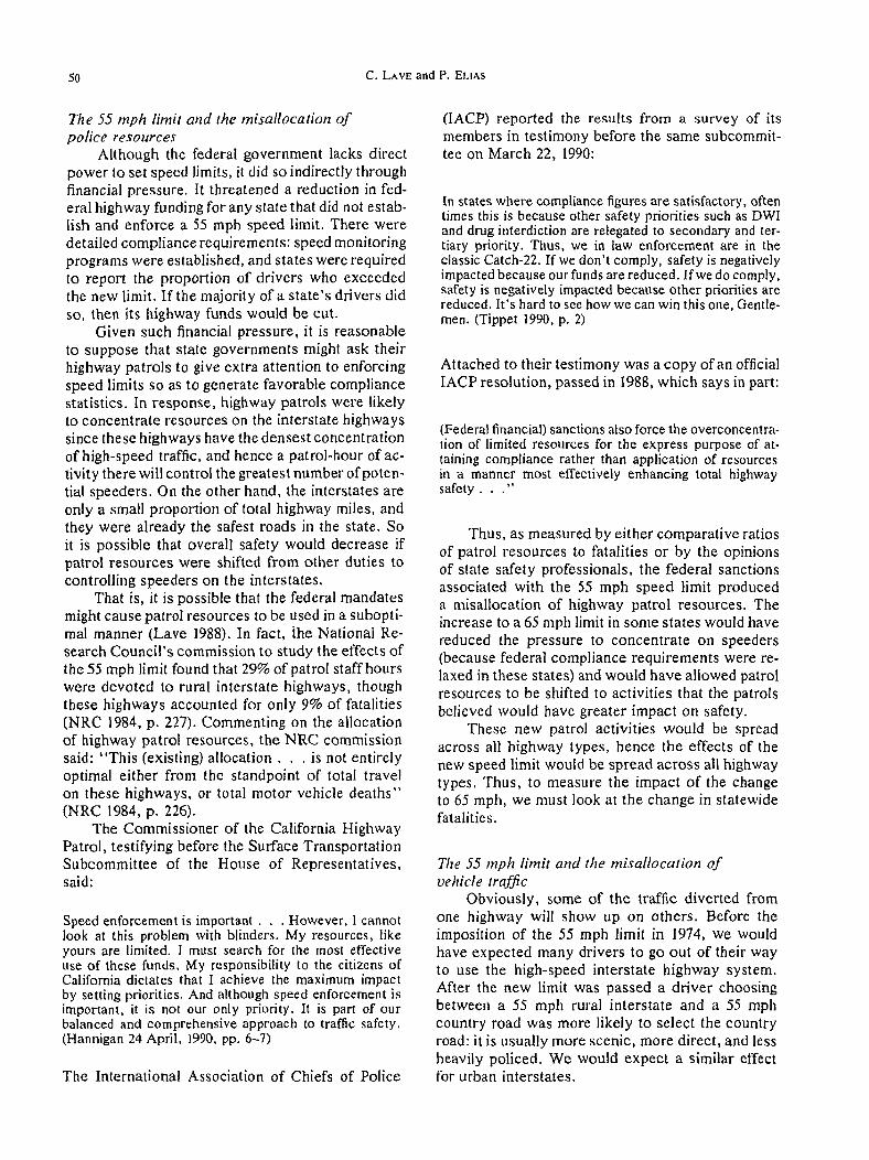
The 55 mph limit and the misallocation ofpolice resources

Although the federal government lacks directpower to set speed limits, it did so indirectly throughfinancial pressure. It threatened a reduction in fed-eral highway funding for any state that did not estab-lish and enforce a 55 mph speed limit. There weredetailed compliance requirements: speed monitoringprograms were established, and states were requiredto report the proportion of drivers who exceededthe new limit. If the majority of a state’s drivers didso, then its highway funds would be cut.

Given such financial pressure, it is reasonableto suppose that state governments might ask theirhighway patrols to give extra attention to enforcingspeed limits so as to generate favorable compliancestatistics. In response, highway patrols were likelyto concentrate resources on the interstate highwayssince these highways have the densest concentrationof high-speed traffic, and hence a patrol-hour of ac-tivity there will control the greatest number of poten-tial speeders. On the other hand, the interstates areonly a small proportion of total highway miles, andthey were already the safest roads in the state. Soit is possible that overall safety would decrease ifpatrol resources were shifted from other duties tocontrolling speeders on the interstates.

That is, it is possible that the federal mandatesmight cause patrol resources to be used in a subopti-mal manner (Lave 1988). In fact, the National Re-search Council’s commission to study the effects ofthe 55 mph limit found that 29% of patrol staffhourswere devoted to rural interstate highways, thoughthese highways accounted for only 9% of fatalities(NRC 1984, p. 227). Commenting on the allocationof highway patrol resources, the NRC commissionsaid: "This (existing) allocation.., is not entirelyoptimal either from the standpoint of total travelon these highways, or total motor vehicle deaths"(NRC 1984, p. 226).

The Commissioner of the California HighwayPatrol, testifying before the Surface TransportationSubcommittee of the House of Representatives,said:

Speed enforcement is important . . . However, I cannotlook at this problem with blinders. My resources, likeyours are limited. I must search for the most effectiveuse of these funds. My responsibility to the citizens ofCalifornia dictates that I achieve the maximum impactby setting priorities. And although speed enforcement isimportant, it is not our only priority. It is part of ourbalanced and comprehensive approach to traffic safety.(Hannigan 24 April, 1990, pp. 6--7)

The International Association of Chiefs of Police

(IACP) reported the results from a survey of itsmembers in testimony before the same subcommit-tee on March 22, 1990:

In states where compliance figures are satisfactory, oftentimes this is because other safety priorities such as DWIand drug interdiction are relegated to secondary and ter-tiary priority. Thus, we in law enforcement are in theclassic Catch-22. If we don’t comply, safety is negativelyimpacted because our funds are reduced. If we do comply,safety is negatively impacted because other priorities arereduced. It’s hard to see how we can win this one, Gentle-men. (Tippet 1990, p. 2)

Attached to their testimony was a copy of an official[ACP resolution, passed in 1988, which says in part:

(Federal financial) sanctions also force the overconcentra-tion of limited resources for the express purpose of at-taining compliance rather than application of resourcesin a manner most effectively enhancing total highwaysafety..."

Thus, as measured by either comparative ratiosof patrol resources to fatalities or by the opinionsof state safety professionals, the federal sanctionsassociated with the 55 mph speed limit produceda misallocation of highway patrol resources. Theincrease to a 65 mph limit in some states would havereduced the pressure to concentrate on speeders(because federal compliance requirements were re-laxed in these states) and would have allowed patrolresources to be shifted to activities that the patrolsbelieved would have greater impact on safety.

These new patrol activities would be spreadacross all highway types, hence the effects of thenew speed limit would be spread across all highwaytypes. Thus, to measure the impact of the changeto 65 mph, we must look at the change in statewidefatalities.

The 55 mph limit and the misallocation ofvehicle traffic

Obviously, some of the traffic diverted fromone highway will show up on others. Before theimposition of the 55 mph limit in 1974, we wouldhave expected many drivers to go out of their wayto use the high-speed interstate highway system.After the new limit was passed a driver choosingbetween a 55 mph rural interstate and a 55 mphcountry road was more likely to select the countryroad: it is usually more scenic, more direct, and lessheavily policed. We would expect a similar effectfor urban interstates.

Did the 65 mph speed limit save lives.’? 51

The overall safety effect of raising the speed lira#The misallocation of traffic and the misalloca-

tion of police resources combine to produce mea-surement bias in the reported safety statistics. Theyoverstate the apparent effect of the 55 mph speedlimit on rural interstate highways: extra policinglowers the fatality rate below what it would be witha 55 mph limit and normal policing; and artificiallydecreased traffic volumes lower the fatality rate be-low what it would be with normal traffic.

What happens on other roads? If patrol re-sources had been misallocated in response to federalpressure to enforce the 55 mph limit, then removingthe federal pressure should cause a better use ofpatrol resources and a decrease in fatalities on nonin-terstate roads. Likewise, any diversion of trafficonto the rural interstates should decrease fatalitieson noninterstate roads (Kamerud 1988; Lave 1988,1989). And McKnight and Klein (1990, p. 77) com-ment: "In the face of widespread noncompliancewith the 55 mph limit, raising the limit on rural Inter-states may benefit safety by diverting some speedersto the highways best able to accommodate them."

Although the competing effects make it difficultto predict the net result of the new speed limit, thetheory does lead to one absolutely unambiguousconclusion:

To evaluate the effect of the increase to 65mph, we must look at total fatality ratesfor the entire state.

III. METHODOLOGY

The estimation of fatality rates is highly sensi-tive to sample size. If some stretch of highway nor-mally has, say, ten fatalities per year, a few randomindividual accidents can greatly affect the apparentfatality rate. Such fluctuations cause serious prob-lems when we are trying to evaluate the effects ofa safety intervention policy: suppose the fatality ratefalls 5%, does that mean the new policy worked? orsuppose the rate remains the same, does that meanthe new policy failed? The answer in both cases is:we just do not know because the expected yearlyfluctuations in these rates are larger than the proba-ble effects from the new policy. Yet a number ofstudies of the new speed limit have relied on smallsamples from a specific highway type within a spe-cific state.

This study analyzes the effect of the new speedlimit using two independent methodologies. First,in Sections IV and V we compare the experience ofthe entire group of states that raised speeds againstthe experience of the states that did not. This resem-

Table 1. Change in statewide fatality rates

The change (%) in statewide fatality rates

Overall change1986->1987 1987-> 1988 1986-> 1988

The 65 mph states -4.68 - i.55 -6.15The 55 mph states -.07 -2.55 -2.62

bles the familiar test group versus control groupmethodology, though obviously it is not a randomsample. Second, in Sections VI and VII we analyzethe data on a state-by-state basis using regressionson monthly time-series data. This enables us to in-corporate the effects of background variables thatmight differ across states.

Both methodologies use the theoretically cor-rect dependent variable: statewide fatalities dividedby statewide VMT.

IV. AGGREGATE METHODOLOGY

We aggregate states into two large groups: thosethat raised the speed limit to 65 mph in 1987 versusthose that did not. For each group of states, wecompute the total fatality rate: the sum of overallstatewide fatalities across the entire group, dividedby the sum of statewide VMT. We do this for 1986,the last full year of data before the change in thespeed limit, and for 1988, the first full year of dataafterwards. To evaluate the effects of the new speedlimit, we compare the change in fatality rates forthe 65 mph states against the change in fatality ratesin the 55 mph states.

In effect, we are comparing a test group to acontrol group. The time period is the same for bothgroups so we are holding constant many of the ef-fects that might be operating on the fatality rate:long-term trends, improvements in auto safety fea-tures, roads, driving habits, or the influence of gen-eral economic changes.* Furthermore, the aggrega-tion into groups of states enhances reliability forthe same reason that an average is a more reliableestimator than a sample of one: the effect of a posi-tive idiosyncratic influence on the fatality rate in onestate, will tend to be canceled by the effect of anegative idiosyncratic influence in another state.

The analysis is based on data compiled by theNational Highway Traffic Safety Administration(NHTSA 1989, pp. 33-44). Table 1 shows the basic

* The procedure cannot correct for any causal factor thatdiffers systematically between the two groups of states. We wereable to eliminate one such possibility: seat belt usage is similar.The 55 mph states had an average belt usage rate of 20.8% in1986 and 48.2% in 1988, a 27.5% improvement. The 65 mph stateshad a belt usage of 24.1% in 1986 and 51.5% in 1988, also a 27.5%improvement.

52 C. LAVE and P. ELIAS

results. Looking at the states that raised their speedlimits in 1987: the overall fatality rate fell by 4.68%in 1987 (compared to the year before when the limithad been 55 mph), and then fell an additional 1.55%in 1988 for an overall drop of 6.15%. Looking atthe states that did not change their speed limits:fatality rates were essentially unchanged in 1987compared to the year before, and then fell by 2.55%the next year for an overall drop of 2.62%.

Obviously we cannot attribute the entire 6.15%fatality drop (in the 65 mph states) to the new speedlimit. Fatality rates might have declined even if thelimit had not changed. There is no absolutely certainway to calculate such a contrafactual estimate, butthere is a way to estimate it by using data from thestates that did not change the speed limit. Considerthem a control group for the 65 mph speed limitexperiment, and use their experience to estimatewhat would have happened to the test group--thestates that did raise the limit. The difference in fatal-ity rates between the two groups of states is 3.62%.(calculated as [100/(100- 2.62)] × [6.15 - 2.62]).That is, we estimate that the 65 mph speed limitreduced the fatality rate by 3.62% compared to thosestates that did not raise their speed limit.

How certain is this result? Its accuracy dependson the truth of the control group assumptions: arethe states that retained the 55 limit generally compa-rable to the states that changed to 65 mph? Manyfactors can influence the fatality rate. To be abso-lutely certain of these conclusions, we would needenormously more data than are available, to holdall those factors constant (Kamerud 1988).

But despite data limitations, this estimate hasseveral significant advantages: (i) it uses a betterevaluation criterion--the effect on the statewide fa-tality rate; (ii) it aggregates the data into largegroups, to produce far more reliable estimates offatality ratesmthey are more stable, and the implicitaveraging process helps to compensate for the ef-fects of excluded idiosyncratic variables as well; (iii)the use of a control group should take care of manyof the remaining problems from excluded variables.

V. ADDITIONAL EVIDENCE

We posit a connection between the misalloca-tion of police resources, the misallocation of traffic,and the overall statewide death rate. The relativedecline in fatality rates (for those states that in-creased the speed limit) supports the theory. Is thereany microlevel evidence as well? For example, arethere data to show that police actually did reallocateresources, or that traffic actually did move betweenhighway types?

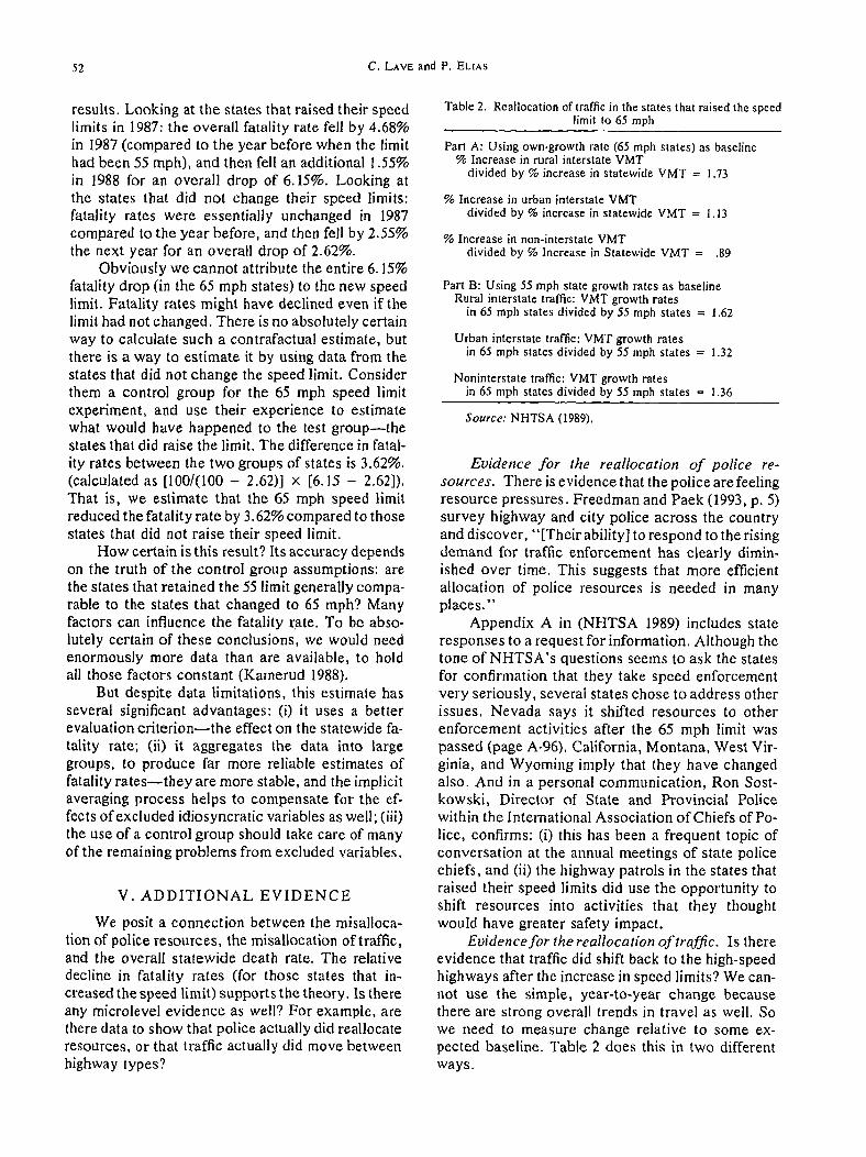
Table 2. Reallocation of traffic in the states that raised the speedlimit to 65 mph

Part A: Using own-growth rate (65 mph states) as baseline% Increase in rural interstate VMT

divided by % increase in statewide VMT = 1.73

% Increase in urban interstate VMTdivided by % increase in statewide VMT = 1.13

% Increase in non-interstate VMTdivided by % Increase in Statewide VMT = .89

Part B: Using 55 mph state growth rates as baselineRural interstate traffic: VMT growth rates

in 65 mph states divided by 55 mph states = 1.62

Urban interstate traffic: VMT growth ratesin 65 mph states divided by 55 mph states = 1.32

Noninterstate traffic: VMT growth ratesin 65 mph states divided by 55 mph states = 1.36

Source: NHTSA (1989).

Evidence for the reallocation of police re-sources. There is evidence that the police are feelingresource pressures. Freedman and Pack (1993, p. 5)survey highway and city police across the countryand discover, "[Their ability] to respond to the risingdemand for traffic enforcement has clearly dimin-ished over time. This suggests that more efficientallocation of police resources is needed in manyplaces."

Appendix A in (NHTSA 1989) includes stateresponses to a request for information. Although thetone of NHTSA’s questions seems to ask the statesfor confirmation that they take speed enforcementvery seriously, several states chose to address otherissues. Nevada says it shifted resources to otherenforcement activities after the 65 mph limit waspassed (page A-96). California, Montana, West Vir-ginia, and Wyoming imply that they have changedalso. And in a personal communication, Ron Sost-kowski, Director of State and Provincial Policewithin the International Association of Chiefs of Po-lice, confirms: (i) this has been a frequent topic conversation at the annual meetings of state policechiefs, and (ii) the highway patrols in the states thatraised their speed limits did use the opportunity toshift resources into activities that they thoughtwould have greater safety impact.

Evidence for the reallocation of traffic. Is thereevidence that traffic did shift back to the high-speedhighways after the increase in speed limits? We can-not use the simple, year-to-year change becausethere are strong overall trends in travel as well. Sowe need to measure change relative to some ex-pected baseline. Table 2 does this in two differentways.

Did the 65 mph speed limit save lives.’? 53

Part A, at the top concentrates on the statesthat increased speed limits to 65 mph. For thesestates, it compares the VMT growth rate on specifichighway types to the overall VMT growth rate inthe state. For example, it shows that traffic on therural interstate highways in the 65 mph states, grew1.73 times faster than the overall VMT growth inthose states. Traffic on the noninterstate highwaysgrew at only 89% of the overall VMT growth ratefor these states. Both results are consistent with ourtheory.

Part A makes internal VMT growth compari-sons: highway type versus the state average. PartB compares the VMT growth in the 65 mph statesto the growth in the 55 mph states, keeping highwaytype constant. Thus, it can be seen that on ruralinterstate highways, VMT grew 1.62 times faster inthe 65 mph states than it did in the 55 mph states.And so on. These numbers are consistent with theexpected pattern of traffic shifts that would be ex-pected if the underlying theory were correct.

To summarize: there is strong evidence thatstate highway patrols wanted to reallocate resourcesin the hypothesized way, and there is some evidencethey actually implemented this intention. And thereis evidence that traffic patterns actually did shift inthe manner we hypothesized.

VI. STATE-BY-STATEREGRESSION ANALYSIS

The results in Section IV contradict the intuitionof many observers and must be examined carefully.The results rely on a comparison in fatality trendsbetween the states that did and those that did notraise their speed limits. The basic assumption behindsuch a test-group/control-group evaluation is thatthe two groups are otherwise comparable. Perhapsthat is not true here: perhaps some economic factorled one group of states to stick with the old speedlimit and also affected their fatality rate. The obviousway around this possibility is to disaggregate thedata and explicitly model the determinants ofthe fatality rate in individual states; then, holdingother factors constant, measure any change in thestate’s fatality rate that occurred after the speedlimit was raised. There is already such a state-by-state analysis in the literature, and we will buildon it.

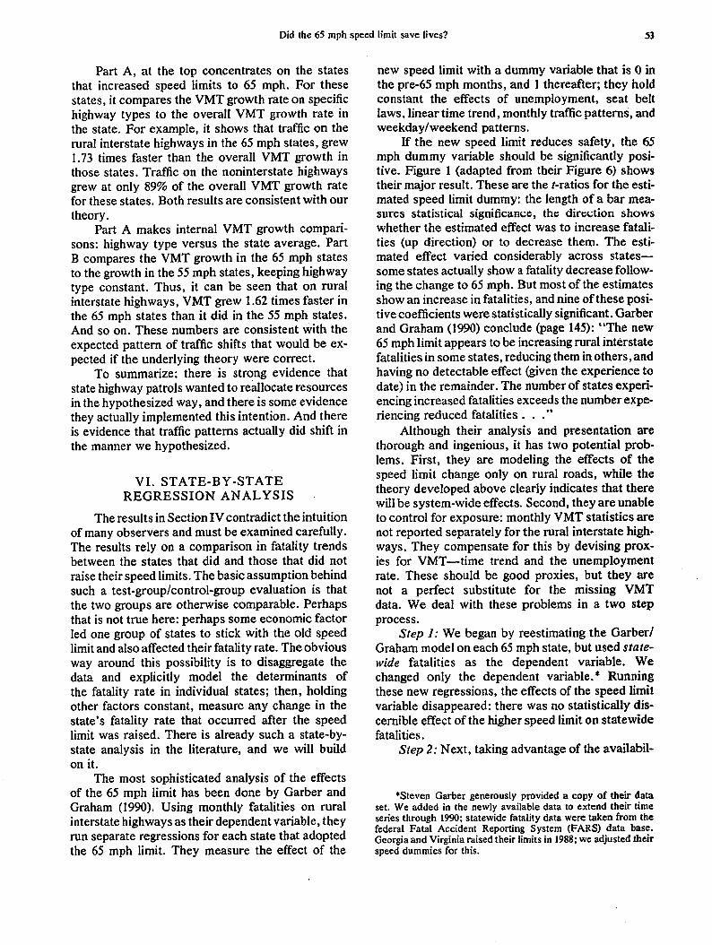
The most sophisticated analysis of the effectsof the 65 mph limit has been done by Garber andGraham (1990). Using monthly fatalities on ruralinterstate highways as their dependent variable, theyrun separate regressions for each state that adoptedthe 65 mph limit. They measure the effect of the

new speed limit with a dummy variable that is 0 inthe pre-65 mph months, and I thereafter; they holdconstant the effects of unemployment, seat beltlaws, linear time trend, monthly traffic patterns, andweekday/weekend patterns.

If the new speed limit reduces safety, the 65mph dummy variable should be significantly posi-tive. Figure 1 (adapted from their Figure 6) showstheir major result. These are the t-ratios for the esti-mated speed limit dummy: the length of a bar mea-sures statistical significance, the direction showswhether the estimated effect was to increase fatali-ties (up direction) or to decrease them. The esti-mated effect varied considerably across states--some states actually show a fatality decrease follow-ing the change to 65 mph. But most of the estimatesshow an increase in fatalities, and nine of these posi-tive coefficients were statistically significant. Garberand Graham (1990) conclude (page 145): "The 65 mph limit appears to be increasing rural interstatefatalities in some states, reducing them in others, andhaving no detectable effect (given the experience todate) in the remainder. The number of states experi-encing increased fatalities exceeds the number expe-riencing reduced fatalities...’"

Although their analysis and presentation arethorough and ingenious, it has two potential prob-lems. First, they are modeling the effects of thespeed limit change only on rural roads, while thetheory developed above clearly indicates that therewill be system-wide effects. Second, they are unableto control for exposure: monthly VMT statistics arenot reported separately for the rural interstate high-ways. They compensate for this by devising prox-ies for VMT--time trend and the unemploymentrate. These should be good proxies, but they arenot a perfect substitute for the missing VMTdata. We deal with these problems in a two stepprocess.

Step 1: We began by reestimating the Garber/Graham model on each 65 mph state, but used state-wide fatalities as the dependent variable. Wechanged only the dependent variable.* Runningthese new regressions, the effects of the speed limitvariable disappeared: there was no statistically dis-cernible effect of the higher speed limit on statewidefatalities.

Step 2: Next, taking advantage of the availabil-

*Steven Garber generously provided a copy of their dataset. We added in the newly available data to extend their timeseries through 1990; statewide fatality data were taken from thefederal Fatal Accident Reporting System (FAR$) data base.Georgia and Virginia raised their limits in 1988; we adjusted theirspeed dummies for this.

54 C. LAVE and P. ELIAS

"1-12..

tf~f.O

OI--

ILl

Z<-1-O

<I

cO

h-

WYOI~WlSC

WVIRGWAShVIRG

VEFI~UTAH

TEXASTENN8DAKSCAROREGOKLAOHIONDAKNCARNMEX~

NHAMP.NEVANEBR"MONT~_MISSQMISSIMINNMICH

MAINELOUISKENTKANSIOWA

II

I II I I

Lll

II I

II

I I JI

I II

I

I

II I

m

I

II

lR

I|

INDI_ILLIIOAH_-

GEOR..FLORCOLO-

CAU

At.AB.-3,00 -2.00 -1.00 0.00 1.00 2.00 3.00 4.00

Value of t-statistic for Speed DummyFig. 1. Garber and Graham (1990) estimate of the effect of increasing speed limits.

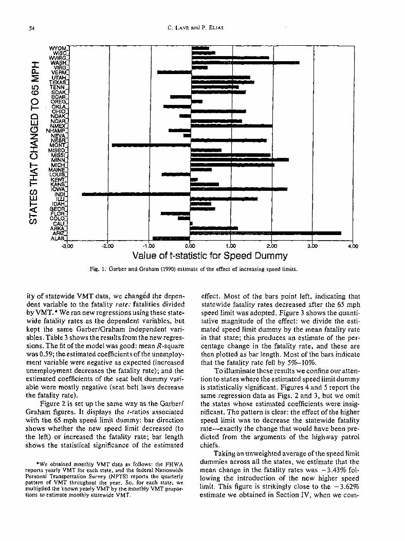
ity of statewide VMT data, we changed the depen-dent variable to the fatality rate: fatalities dividedby VMT.* We ran new regressions using these state-wide fatality rates as the dependent variables, butkept the same Garber/Graham independent vari-ables. Table 3 shows the results from the new regres-sions. The fit of the model was good: mean R-squarewas 0.59; the estimated coefficients of the unemploy-ment variable were negative as expected (increasedunemployment decreases the fatality rate); and theestimated coefficients of the seat belt dummy vari-able were mostly negative (seat belt laws decreasethe fatality rate).

Figure 2 is set up the same way as the Gather/Graham figures. It displays the t-ratios associatedwith the 65 mph speed limit dummy: bar directionshows whether the new speed limit decreased (tothe left) or increased the fatality rate; bar lengthshows the statistical significance of the estimated

*We obtained monthly VMT data as follows: the FHWAreports yearly VMT for each state, and the federal NationwidePersonal Transportation Survey (NPTS) reports the quarterlypattern of VMT throughout the year, So, for each state, wemultiplied the known yearly "qMT by the monthly ’qMT propor-tions to estimate monthly statewide VMT.

effect. Most of the bars point left, indicating thatstatewide fatality rates decreased after the 65 mphspeed limit was adopted. Figure 3 shows the quanti-tative magnitude of the effect: we divide the esti-mated speed limit dummy by the mean fatality ratein that state; this produces an estimate of the per-centage change in the fatality rate, and these arethen plotted as bar length. Most of the bars indicatethat the fatality rate fell by 5%--10%.

To illuminate these results we confine our atten-tion to states where the estimated speed limit dummyis statistically significant. Figures 4 and 5 report thesame regression data as Figs. 2 and 3, but we omitthe states whose estimated coefficients were insig-nificant. The pattern is clear: the effect of the higherspeed limit was to decrease the statewide fatalityrate--exactly the change that would have been pre-dicted from the arguments of the highway patrolchiefs.

Taking an unweighted average of the speed limitdummies across all the states, we estimate that themean change in the fatality rates was -3.43% fol-lowing the introduction of the new higher speedlimit. This figure is strikingly close to the -3.62%estimate we obtained in Section IV, when we com-

Did the 65 mph speed limit save lives.’?

Table 3. Results from regression on states adopting 65 mph limit (1976-1990 data)

55

65 mph Mean ofspd lim Percent Belt use fatality

State dummy t ratio unemploy t ratio dummy t ratio r2 rate

Alabama - 0.0014 - 0.89 - 0.00054 - 2.98 0.650 0.031Arizona - 0.0099 - 5.81 - 0.00243 - 8.29 0.761 0.04 lArkansas - 0.0005 - 0.24 - 0.00005 0.12 0.516 0.034California -0.0018 -2.28 -0.00134 -8.11 -0.00127 - 1.51 0.859 0.028Colorado -0.0025 -0.76 -0.00024 -0.60 0.00411 1.20 0.724 0.027Florida - 0.0034 - 2.70 - 0.00093 - 3.78 - 0.00355 - 2.70 0.747 0.033Georgia 0.0008 0.53 - 0.00221 - 7.59 - 0.00382 - 2.41 0.774 0.029Idaho - 0.0026 - 0.56 - 0.00061 - 0.93 0.00388 0.98 0.569 0.036Illinois 0.0022 1.93 -0.00047 -2.46 0.00070 0.61 0.808 0.026Indiana 0.0025 0.53 -0.0001 ! -0.63 -0.00453 -0.99 0.680 0.026Iowa 0.0047 2.01 - 0.00060 - 1.37 0.00005 0.02 0.667 0.028Kansas -0.0016 -0.75 -0.00097 - 1.69 -0.00105 -0.50 0.604 0.028Kentucky 0.0025 1.56 0.00026 1.22 0.662 0.030Louisiana -0.0017 -0.57 -0.00044 - !.07 -0.00065 -0.22 0.689 0.038Main - 0.0015 - 0.66 - 0.00021 - 0.37 0.444 0.026Michigan 0.0005 0.61 -0.00034 -3.14 -0.00030 -0.29 0.821 0.025Minnesota 0.0017 1.08 -0.00153 -5.25 -0.00222 - 1.36 0.817 0.022Mississippi -0.0703 - 1.96 -0.01293 -2.38 -0.02880 -0.74 0.089 0.065Missouri 0.0044 2.14 -0.00099 -2.33 0.00044 0.18 0.465 0.030Montana -0.0094 - 1.70 - 0.00111 - 1.26 0.00528 0.92 0.562 0.037Nebraska -0.0018 -0.80 - 0.00111 - 1.97 0.466 0.025Nevada -0.0096 - i.36 -0.00179 -3.51 0.01067 1.53 0.534 0.041New Hampshire - 0.0051 - 2.57 - 0.00053 - 1.33 0.520 0.024New Mexico - 0.0013 - 0.45 - 0.00089 - 1.76 0.00012 0.04 0.674 0.045North Carolina -0.0026 -2.23 -0.00047 - 1.96 0.00081 0.61 0.770 0.032North Dakota 0.0149 0.56 0.00829 0.93 -0.00624 -0.17 0.108 0.041Ohio 0.0002 0.21 - 0.00053 - 3.72 - 0.00084 - 0.72 0.757 0.024Oklahoma -0.0109 -0.17 -0.00762 - 1.63 -0.01796 -0.28 0.090 0.050Oregon 0.0004 0.26 - 0.00055 - 2.32 0.00088 0.57 0.678 0.030South Carolina - 0.0033 - 1.97 - 0.00081 - 3.19 - 0.00473 - 2.85 0.592 0.036South Dakota 0.0043 1.23 - 0.00048 - 0.40 0.458 0.028Tennessee -0.0026 - 1.68 -0.00047 -2.29 0.00101 0.66 0.695 0.032Texas -0.0029 -2.66 -0.00131 -5.21 -0.00288 -2.60 0.859 0.030Utah - 0.0047 - 1.90 - 0.00098 - 2.33 0.00223 0.91 0.535 0.028Vermont - 0.0000 - 0.01 - 0.00243 - 3.16 0.429 0.028Virginia 0.0004 0.30 -0.00090 -3.22 -0.00135 -0.90 0.780 0.023Washington -0.0015 -0.97 -0.00132 -6.20 -0.00078 -0.53 0.777 0.025West Virginia 0.0001 0.02 -0.00019 -0.77 0.485 0.038Wisconsin -0.0018 -0.81 -0.00040 - 1.93 0.00170 0.78 0.742 0.024Wyoming 0.0031 0.86 - 0.00111 - 1.65 -0.00264 -0.70 0.713 0.038

Linear regressions set up as in Garber & Graham, including dummy variables for months.Dependent variable = Monthly statewide fatality rate, that is: (monthly fatalities on all road types)/(statewide monthly VMT).

pared the change in aggregate fatalities between thestates that did and did not adopt the new speed limit.

The results in Section IV rely on aggregate anal-ysis: we compute the overall fatality rate for thecombined 65 mph sample of states before and afterthe new speed limit; then this is compared to thetime trend in the overall fatality rate for the statesthat did not adopt the new limit, using them as acontrol group to hold other factors constant. Theresults in this section compute the change in fatali-ties on a state-by-state basis, while explicitly holdingconstant the effects of time trends, unemployment,seat belt laws, and traffic patterns. Given the sub-stantial difference in methodologies, the similarityof results lends confidence to the conclusions.

Step 3: As an additional check on the regres-sions, we examined an alternative hypothesis. Sup-pose there had been a nationwide break in fatalitytrends starting in 1987--for some reason other thanthe new speed limit--and that fatality rates had be-gun an overall drop after that time. If this were true,then the 65 mph speed limit dummy would pick upthe effect of this trend break and be spuriously nega-tive. The significance of the dummy would reflectthe overall break in fatality trends, not the changein the speed limit laws.

If there had been such a spurious break in thetime trend, we would detect its effect in data fromstates that did not raise speed limits. So we did thefollowing: using the states that had not raised their

56 C. LAVE and P. ELIAS

"i-D_

u3CO)

0

LU

z<"r-

Op-<-r"F-iiiF-

O0

WYOMwIsc-

WVIRGWAShVIRG

VERM"UTAH

TEXASTENN8DAKSCAROREGOHIONCARNMEX

NHAMPNEVA’NEBRMONTMISSO

MINN-MICH-

MAINE"LOUIS"KENT"KANS"IOWA"

INDI-ILLI"

IDAH-GEOR-FLOR-COLO-

CALl-ARKA-ARIZ-ALAB-

mi

m

|

II

I Illll

I Ill

mq III

I

mIm

m

mI

l.

|

II

BB_ _. i_~J_

-6.00 -5.00 -4,0( -3,00 -2.00 -1.00 0.00 1.00 2.00 3.00

Value of t-statistic for Speed DummyFig. 2. T-value of 65 mph speed limit. Coeff; Dep. Var = Fatality rate 1976-1990.

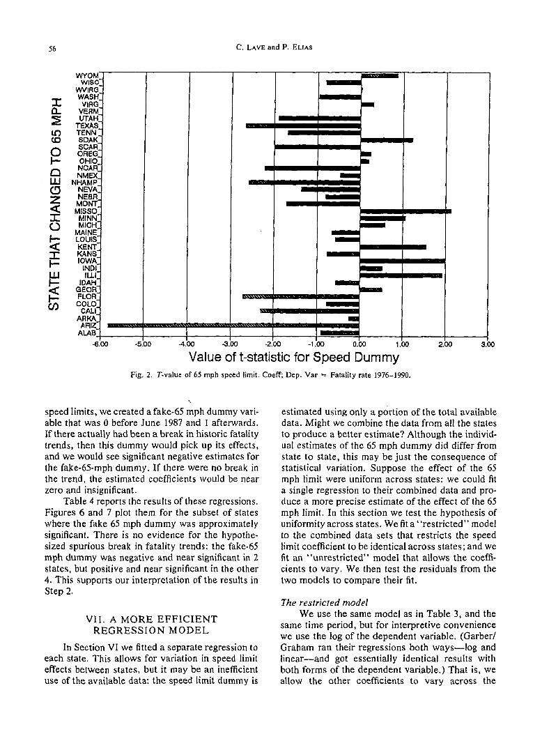
speed limits, we created a fake-65 mph dummy vari-able that was 0 before June 1987 and 1 afterwards.If there actually had been a break in historic fatalitytrends, then this dummy would pick up its effects,and we would see significant negative estimates forthe fake-65-mph dummy. If there were no break inthe trend, the estimated coefficients would be nearzero and insignificant.

Table 4 reports the results of these regressions.Figures 6 and 7 plot them for the subset of stateswhere the fake 65 mph dummy was approximatelysignificant. There is no evidence for the hypothe-sized spurious break in fatality trends: the fake-65mph dummy was negative and near significant in 2states, but positive and near significant in the other4. This supports our interpretation of the results inStep 2.

VII. A MORE EFFICIENTREGRESSION MODEL

In Section VI we fitted a separate regression toeach state. This allows for variation in speed limiteffects between states, but it may be an inefficientuse of the available data: the speed limit dummy is

estimated using only a portion of the total availabledata. Might we combine the data from all the statesto produce a better estimate? Although the individ-ual estimates of the 65 mph dummy did differ fromstate to state, this may be just the consequence ofstatistical variation. Suppose the effect of the 65mph limit were uniform across states: we could fita single regression to their combined data and pro-duce a more precise estimate of the effect of the 65mph limit. In this section we test the hypothesis ofuniformity across states. We fit a "restricted" modelto the combined data sets that restricts the speedlimit coefficient to be identical across states; and wefit an "unrestricted" model that allows the coeffi-cients to vary. We then test the residuals from thetwo models to compare their fit.

The restricted modelWe use the same model as in Table 3, and the

same time period, but for interpretive conveniencewe use the log of the dependent variable. (Garber/Graham ran their regressions both ways--log andlinear--and got essentially identical results withboth forms of the dependent variable.) That is, weallow the other coefficients to vary across the

Did the 65 mph speed limit save lives? 57

WYOMwise

WVIRGWASHVIRG

VERMUTAH

TEXASTENNSDAKSCAROREGOHIONCARNMEX

NHAMFNEVA_NEBFMONT_MISSO_MINN_MICH_

MAINELOUIS_KENT_KANS_IOWA_INDI_ILL

IDAH_GEOR_FLOR_COLO_CAL

ARKA_ARIZ_ALAB_

-30.00% -25.00%

I

I

I

I

II

m

1 11

-20.00% -15.00% -I 0.00% -5.00% 0.00% 5.00% 10.00%

Coeff.Estimate / Mean of Fatality RataFig. 3. Estimated % change in fatality rates after increase to 65 mph limit.

15.00%

states--they are allowed to have different timetrends, seat belt effects, unemployment effects, andso on--but we estimate a single 65 mph dummy forthe entire 40-state sample. Observations span theperiod from January 1976 to December 1990. Thusthere were 7,200 observations, 180 from each state.

Since the dependent variable is in logs, the esti-mated coefficient for the speed limit variable is thepercentage change in fatality rate, nationwide. Re-sults of the restricted model are: a 5.06% decreasein fatality rate, with a t-ratio of 3.19. R-squared is0.61.

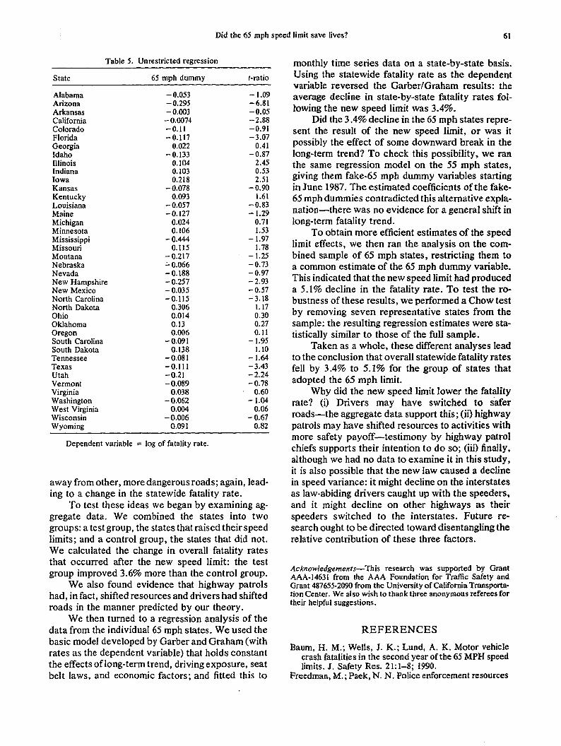
The unrestricted modelThe unrestricted model is identical with the re-

stricted model with one change: the coefficient ofthe speed limit dummy is allowed to vary acrossstates--and each of the unrestricted regressions isfitted to a much smaller data base, only 180 observa-tions. The results of the unrestricted regressions are

shown in Table 5.To evaluate the hypothesis of uniform effect,

we test the fit of the restricted model against theunrestricted model. We perform an F-test on the

residuals, as follows:

F (e’,e. - e’ e)l(g - j)e ’e /j

Where: e’e. is the residual sum of squares of therestricted regression, and g is the degrees of freedomassociated with the restricted regression (equal tothe number of observations minus the number ofcoefficients estimated). And in the denominator: e’eis the residual sum of squares of the unrestrictedregression, andj is the degrees of freedom associatedwith this regression. This produces the F-statistic1.14, with 39 degrees of freedom in the numeratorand 6,520 degrees of freedom in the denominator.That is, we conclude at the 95% level of significancethat the explanatory power of the model is not com-promised by assuming a uniform effect for the newspeed limit across all the states that adopted it. Thisresult also strengthens the conclusion that the newspeed limit decreased the fatality rate.

How robust are these results? Do they reallypresent a general indication of the effects of thenew speed limit, or are they just the result of theparticular combination of data in our sample. Oneway to check the solidity of the results is to alterthe sample, reestimate the regressions and use a

58 C. LAVE and P. ELIAS

.

UTAH¢/)LU TEXAS3 -<~ TENN

"~ SCAR-I.L:

NOAR-z .

~ NHAMP60 -

MONT.MISSO

r,.D KENTW

-6.00 -5.00 -4.00 -3.00 -2.00 -1.00 0.00

re=ms=

1.00

Value of t-statistic for Speed DummyFig. 4. T-value of 65 mph speed limit. Coeff; Dep. Var. = Fatality rate 1976-1990.

2.00 3.00

Chow test to see whether the new estimates aresimilar to the originals. If the two regressions pro-duce widely divergent parameter estimates, thiscasts doubt on the reliability of the model; if the tworegressions produce similar parameter estimates,this lends credibility to the basic estimates.

We performed the test as follows. First, sevenrepresentative states were removed from the sam-ple,* and the restricted model was reestimated fromthe 5,940 observations on the remaining 33 states.The resulting regression coefficients were similar,adjusted R-squared was 0.54, and the 65 mph speedlimit coefficient was estimated at - 4.40%, with a t-ratio of 2.38.

Next, analysis of variance techniques are em-ployed to test the consistency of the two results. AnF-statistic is computed as follows:

*Randomness being impossible to achieve from such a smallpopulation, we instead chose a representative sample: each majorregion of the United States was represented, as were urban andrural states, states that did and did not enact seatbelt laws, andstates whose individual regressions got high and low R-squares.We removed: California, Georgia, Louisiana, Minnesota,Nebraska, New Hampshire, and New Mexico.

F (e" e. - e’ e)/(m - e’e/p

Where: ele. is the residual sum of squares of theoriginal 40-state regression; and m is the degrees offreedom associated with that regression. And in thedenominator: e’e is the residual sum of squares ofthe 33-state regression, and p is the associated de-grees of freedom. This produces an F-statistic of1.07, with 591 degrees of freedom in the numeratorand 6,531 degrees of freedom in the denominator.

That is, the parameter estimates are similar de-spite the large change in the data sample. Thus thereis further reason to believe in the generality of theresults.

VIII. SUMMARY AND CONCLUSIONS

Prior studies of the 65 mph limit have only mea-sured the local effects of the change. But enforce-ment and highways are integrated, interactive sys-tems: extra policing resources used to reducespeeding must be diverted from other kinds of safetyactivities; drivers discouraged from using interstate

Did the 65 mph speed limit save lives? 59

UTAH

TEXAS

\\.~\\\-?~\ \ , ,,. TENN

SCAR_~NCAR

NHAMP

MONT

MISSO

KENT

IOWA

ILLI

FLOR

CALl

ARIZ

-30.00%

B

| NNNNNNNNN x,X’ w NNNNN

mqmm,xNN\NNNN~ ~ ~

10.00% 15.00% 20.00%-25.00% -20.00% -15.00% -10.00% -5.00% 0.00% 5.00%

Value of t-statistic for SpeedDummyFig. 5. Estimated % change in fatality rates after increase to 65 mph limit.

highways may move to other, more dangerousroads. A decrease in fatalities in an area where re-sources have been concentrated may be offset-evenoverwhelmed-by the effects on the rest of the high-way system. Thus, a new speed limit must be evalu-ated by its system-wide consequences. We must useoverall statewide fatality rates as the dependentvariable.

The new 65 mph limit allowed state highwaypatrols to shift resources from speed enforcementon the interstates to other safety activities and otherhighways~a shift many highway patrol chiefs hadargued for. If the chiefs were correct, the realloca-tion of patrol resources should lead to a reductionin statewide fatality rates. In addition, the higherspeed limit on the interstates might attract drivers

Table 4. Regression on states with 55 mph limit, using "fake" 65 mph dummy

Fake 65 mph Mean ofspeed limit Belt use fatality

State dummy var. t-ratio % unemployed t-ratio dummy t-ratio R-sq rate

Alaska - 0.00632 - 1.38 - 0.00073 - 0.69 0.00168 0.29 0.437 0.032

Connecticut - 0.00236 - 1.55 - 0.00111 - 3.39 -0.003 l0 - 1.92 0.565 0.022

Delaware 0.00381 1.50 0.00023 0.38 0.279 0.026

Hawaii 0.00565 1.92 - 0.00154 - 2.02 - 0.00049 - 0.16 0.474 0.027

Maryland - 0.00200 - i .48 - 0.00022 - 0.77 0.00200 1.39 0.617 0.023

Massachusetts 0.00157 1.46 - 0.00111 - 5.45 0.00124 0.90 0.661 0.020

New Jersey - 0.00045 - 0.61 - 0.00052 - 2.70 - 0.00061 - 0.73 0.688 0.020

New York 0.00205 2.32 - 0.00083 - 2.91 - 0.00175 - 1.78 0.826 0,027

Pennsylvania 0.00238 1.88 -0.00040 -2.89 -0.00331 -2.79 0.786 0.026

Rhode Island -0.00520 -0.34 - 0.00122 -0.45 0.053 0.033

Linear regressions set up as in Garber and Graham, including dummy variables for months.Dependent variable = Monthly statewide fatality rate, that is: (monthly fatalities on all road types)/(statewide monthly VMT).

60 C. LAVE and P. ELIAS

t J)OI---

I--Z<LLZ

07

COLU

07LOLO

PENN

NYR~

MASS

MARY

DELA

CONN

f f-2 -1.5 -1 -0.5 0 0.5 1 1.5 2 2.5

DepVar= Statewide Fatality Rate 1976-90Fig. 6. T-ratio of fake 65 mph dummy for states with 55 mph speed limit.

PENN~

~0"~ I NYRKH

CONN. ~_¯ ~ ,-15.00% ~10.00% -5.00% 0.00% 5.00% 10.00% 15.00%

Coef.Est. / Mean Fatality RateFig. 7. Estimated change in fatalities in period following fake 65 mph dummy.

Did the 65 mph speed limit save lives? 6I

Table 5. Unrestricted regression

State 65 mph dummy t-ratio

Alabama - 0.053 - 1.09Arizona - 0.295 - 6.81Arkansas - 0.003 - 0.05California - 0.0074 - 2.88Colorado - 0.11 - 0.91Florida - 0.117 - 3.07Georgia 0.022 0.41Idaho - 0.133 - 0.87Illinois O. 104 2.45Indiana 0.103 0.53Iowa 0.218 2.51Kansas - 0.078 - 0.90Kentucky 0.093 i .61Louisiana - 0.057 - 0.83Maine - 0.127 - 1.29Michigan 0.024 0.71Minnesota 0.106 1.53Mississippi - 0.444 - 1.97Missouri 0.115 1.78Montana - 0.217 - 1.25Nebraska - 0.066 - 0.73Nevada - 0.188 - 0.97New Hampshire - 0.257 - 2.93New Mexico - 0.035 - 0.57North Carolina - 0. I i 5 - 3.18North Dakota 0.306 I. 17Ohio 0.014 0.30Oklahoma 0.13 0.27Oregon 0.006 0. I iSouth Carolina -0.091 - 1.95South Dakota 0.138 1.10Tennessee - 0.081 - 1.64Texas - 0. I I 1 - 3.43Utah - 0.21 - 2.24Vermont - 0.089 - 0.78Virginia 0.038 0.60Washington - 0.062 - 1.04West Virginia 0.004 0.06Wisconsin - 0.006 - 0.67Wyoming 0.091 0.82

Dependent variable = log of fatality rate.

away from other, more dangerous roads; again, lead-ing to a change in the statewide fatality rate.

To test these ideas we began by examining ag-gregate data. We combined the states into twogroups: a test group, the states that raised their speedlimits; and a control group, the states that did not.We calculated the change in overall fatality ratesthat occurred after the new speed limit: the testgroup improved 3.6% more than the control group.

We also found evidence that highway patrolshad, in fact, shifted resources and drivers had shiftedroads in the manner predicted by our theory.

We then turned to a regression analysis of thedata from the individual 65 mph states. We used thebasic model developed by Garber and Graham (withrates as the dependent variable) that holds constantthe effects of long-term trend, driving exposure, seatbelt laws, and economic factors; and fitted this to

monthly time series data on a state-by-state basis.Using the statewide fatality rate as the dependentuariable reversed the Garber/Graham results: theaverage decline in state-by-state fatality rates fol-lowing the new speed limit was 3.4%.

Did the 3.4% decline in the 65 mph states repre-sent the result of the new speed limit, or was itpossibly the effect of some downward break in thelong-term trend? To check this possibility, we ranthe same regression model on the 55 mph states,giving them fake-65 mph dummy variables startingin June 1987. The estimated coefficients of the fake-65 mph dummies contradicted this alternative expla-nation-there was no evidence for a general shift inlong-term fatality trend.

To obtain more efficient estimates of the speedlimit effects, we then ran the analysis on the com-bined sample of 65 mph states, restricting them toa common estimate of the 65 mph dummy variable.This indicated that the new speed limit had produceda 5.1% decline in the fatality rate. To test the ro-bustness of these results, we performed a Chow testby removing seven representative states from thesample: the resulting regression estimates were sta-tistically similar to those of the full sample.

Taken as a whole, these different analyses leadto the conclusion that overall statewide fatality ratesfell by 3.4% to 5.1% for the group of states thatadopted the 65 mph limit.

Why did the new speed limit lower the fatalityrate? (i) Drivers may have switched to saferroads--the aggregate data support this; (ii) highwaypatrols may have shifted resources to activities withmore safety payoff--testimony by highway patrolchiefs supports their intention to do so; (iii) finally,although we had no data to examine it in this study,it is also possible that the new law caused a declinein speed variance: it might decline on the interstatesas law-abiding drivers caught up with the speeders,and it might decline on other highways as theirspeeders switched to the interstates. Future re-search ought to be directed toward disentangling therelative contribution of these three factors.

Acknowledgernents--This research was supported by GrantAAA-14631 from the AAA Foundation for Traffic Safety andGrant 487655-2090 from the University of California Transporta-tion Center. We also wish to thank three anonymous referees fortheir helpful suggestions.

REFERENCES

Baurn, H. M.; Wells, J. K.; Lund, A. K. Motor vehiclecrash fatalities in the second year of the 65 MPH speedlimits. J. Safety Res. 21:1-8; 1990.

Freedman, M.; Paek, N. N. Police enforcement resources

62 C. LAVE and P. ELIAS

in relation to need: Changes during 1978-89. InsuranceInstitute for Highway Safety, January 1993.

Garber, S.; Graham, J. The effects of the new 65 mile-per-hour speed limit on rural highway fatalities: A state-by-state analysis. Accid. Anal. Prey. 22:137-149; 1990.

Gallagher, M. M.; Sewell, N.; Herndon, J. L.; Graft, N.;Flenner, J.; Hull, H. F. Effects of the 65 MPH speedlimit on rural interstate fatalities in New Mexico. J. A.M. A. 262:2234-2245, 1989.

Hannigan, M. J. Statement for the record, prepared forSanctions Conference, Sacramento, CA, June 21,1990.

Kamerud, D. B. Evaluating the new 65 mph speed limit.pp. 231-256 In: John D. Graham, editor. Preventingautomobile injury. Dover, MA: Auburn House Publish-ing Company; 1988: pp. 231-256.

Lave, C. The 55 MPH speed limit on U.S. roads: Corn-

ments on Godwin and Kulash’s analysis. TransportReviews 8:237-244; 1988.

Lave, C. Speeding, coordination, and the 55-MPH limit:reply, American Economic Review 79:926-936, 1989.

McKnight, A. J.; Klein, T. M. Relationship of 65 mphlimit to speeds and fatal accidents. Transp. Res. Rec.1281:71-77; 1990.

NHTSA. The effects of the 65 mph speed limit through1988: A report to Congress. Washington DC: NationalHighway Traffic Safety Administration, U.S. Depart-ment of Transportation; October 1989.

NRC. 55: A decade of experience. Washington DC: Na-tional Research Council of the National Academy ofSciences; 1984.

Tippet, E. Testimony before the Subcommittee on PublicWorks and Surface Transportation of the U.S. Houseof Representatives, April 24, 1990.