characterization of soil fertility using the rasch model

486

Journal of Soil Science and Plant Nutrition, 2017, 17 (2), 486-498

RESEARCH ARTICLE

Characterization of soil fertility using the Rasch model

Francisco J. Moral1*, Francisco J. Rebollo2

1Departamento de Expresión Gráfica, Escuela de Ingenierías Industriales, Universidad de Extremadura. Avda. de Elvas, s/n. 06071, Badajoz, Spain. 2Departamento de Expresión Gráfica, Escuela de Ingenierías Agrar-ias, Universidad de Extremadura. Avda. Adolfo Suárez s/n, 06007, Badajoz, Spain. *Corresponding author: [email protected]

Abstract

A quantification of the overall soil fertililty potential should integrate the main soil physical and chemical prop-erties, with different units. The formulation of the Rasch model is proposed as an instrument to measure soil fertility potential, integrating 11 soil properties (clay, silt and sand content, organic matter -OM-, pH, total ni-trogen -TN-, available phosphorus -AP- and potassium -AK-, cation exchange capacity -CEC-, and deep -ECd- and shallow -ECs- soil apparent electrical conductivity, 0-90 and 0-30 cm depth respectively) measured at 70 locations in a field. In the case study, the considered soil variables fit the model reasonably, having an important influence on soil fertility, except pH, probably due to its homogeneity in the field. Moreover, a ranking of all soil samples according to their fertility potential and the influence of each variable on soil fertility are provided, being ECd, ECs, and the textural fractions of soil the most influential properties on soil fertility and, on the other hand, AP and AK the less influential properties. Results are in accordance with a previous work in the same field considering only five soil properties, both ECd and ECs and texture, denoting the importance of these variables to estimate soil fertility potential. Rasch model resulted to be useful to rationally determine locations in a field where high soil fertility potential exists and establishing those soil samples or properties with anomalies. This information can be necessary to conduct site-specific treatments, leading to a more cost-effective and sustainable field management.

Keywords: Nutrients, texture, Rasch model, soil apparent electrical conductivity


487Characterization of soil fertility using the Rasch model

1. Introduction

Soil fertility is a complex quality of soils which is clos-est to plant nutrient management. It combines many biological, chemical and physical soil properties that affect nutrient availability. Although soil fertility is one important aspect of soil productivity, from the farmer´s point of view the chemical fertility and physical condi-tion of soils are decisive as they both determines the production potential. Good natural or improved soil fertility is indispensable for successful cropping and the basis for any high-production system.According to FAO, soil fertility can be defined as the ability of a soil to supply the essential nutrients and adequate amounts of soil water to plant growth (http://www.fao.org/ag/agp/agpc/doc/publicat/FAOBUL4/FAOBUL4/B401.htm). The requirements of plants should be met from the elements contained in the soil; thus, initially, it has a fertility potential, but some oth-er factors have to be taken into account.Quantifying soil fertility in a meaningful way is very problematic. In order to estimate it, three main prob-lems can be distinguished: i) What shall we measure? ii) How do we interpret the data? iii) How can we de-rive a statement about soil fertility based on the data?Several soil properties are important in determining a soil's inherent fertility. One property is the adsorp-tion and storage of nutrients on the surfaces of soil particles. The quantity of nutrient cations a soil can adsorb is called its cation exchange capacity (CEC). Soils with high CEC not only hold more nutrients, but they are better able to buffer, or avoid rapid changes in soil solution levels of these nutrients by replacing them as the solution become depleted. Generally, the inherent fertility, and long-term productivity of a soil is greatly influenced by its CEC.Depending on its location, a soil contains some com-bination of sand, silt, clay, and organic matter. The makeup of a soil (soil texture) and its acidity (pH)

determine the extent to which nutrients are available to plants. Soil texture affects how well nutrients and water are retained in the soil; thus, clayey and organic soils hold nutrients and water much better than sandy soils, in which water drains and carries nutrients along with it. When nutrients leach into the soil, they are not available for plants to use. Thus, soil texture and CEC are related; for instance, soils with high CEC usually have high clay content, moderate to high organic mat-ter content, high water holding capacity, less frequent need for fertilizers, and low leaching potential for cat-ionic nutrients. However, an ideal soil should contain equivalent portions of sand, silt, and clay, to facilitate the agricultural works as the physical properties are more adequate to properly manage the soil.Soil pH is one of the most important soil properties that affect the availability of nutrients (e.g. Nájera et al., 2015; Li et al., 2015). The ideal soil pH is close to neutral. Most plant nutrients are optimally available to plants within this 6.5 to 7.5 pH range, plus this range of pH is generally very compatible to plant root growth.Soil apparent electrical conductivity (ECa) is another soil property closely related to some important physi-co-chemical properties influencing crop yield across a wide range of soils (e.g. Corwin and Lesch, 2003; Sud-duth et al., 2005). High correlation coefficients have been found between ECa and other variables related to soil fertility as CEC and pH (e.g., Bernardi et al., 2016; Moral et al., 2010). In this sense, ECa measurements can be considered an indicator of soil-fertility param-eters. ECa can be intensively recorded in a parcel, in an easy and inexpensive way, by means of different electrical conductivity sensors currently on the market (e.g. Pedrera-Parrilla et al., 2016).In consequence, obtaining a measure of soil fertility po-tential is not easy due to the fact that different variables


488 Moral et al.

can influence its quantification. Soil fertility is af-fected by many soil physical and chemical variables, which, in turn, depend on various local factors, such as climatological conditions. Another additional problem is the correct choice of the variables that can better characterize the soil fertility. If soil texture properties, CEC, pH, primary nutrients availability and apparent electrical conductivity (ECa) are con-sidered, it seems that a rational indication about the soil fertility potential can be obtained (e.g. Serrano et al., 2016). However, how do we combine these variables? It seems like a puzzle with pieces out of different pictures; the pieces do not match, no pic-ture emerges. Soil fertility is a complex property not expressed appropriately in a quantitative way.A novel approach to integrate data from different variables is the Rasch model (Rasch, 1980), which is an objective and statistical measurement model. The useful information this statistical tool can generate can give new insight from an agricultural point of view. Moral et al. (2012) applied the Rasch model to obtain rational measures of soil fertility potential in a field, from ECa and textural components obtained at some soil samples. It was obtained that ECa was the most influential property on soil fertility potential. However, other soil variables, for instance primary nutrients availability, were not considered. Addition-ally, in a previous work, Moral et al. (2011) used the Rasch model and some geostatistical algorithms with the aim of delineating different management zones in an agricultural field, considering five soil properties (clay, silt and sand content, ECd, and ECs) as the most influential on soil fertility. However, no additional information was displayed regarding how the data fit the model, if results are consistent and all variables support the latent variable, or if the number of categories is the optimum, that is, if the rating scale categories are being used appropriately. Furthermore, the study of misfits was not included,

which could be an important source of information about anomalies in any soil property or data at every sample location.The Rasch model, as a measuring method (Tristán, 2002; Álvarez, 2004), can be an important and in-novative tool to determine soil fertility potential (in the sense the crop production potential is influenced by soil fertility). This latent variable model is based on the mathematical modeling of the behaviour re-sulting from the iteration of a subject with its item (Tristán, 2002). It is a single parameter model, i.e., there is only one measurement parameter, which cor-responds to a single dimension on a single scale to measure the classification of both the subjects (soil samples) and the considered items (soil properties). The Rasch model can integrate different data into a uniform analytical framework. In this case study, the main purpose is to consolidate some heterogeneous measures of soil properties into an overall variable that characterizes and facilitates the interpretation of potential fertility in an agricultural soil.This model is also based on the simple idea that some items are more important to subjects than other items. Thus, the Rasch model constructs a line of measurement with the items located hierarchically on this line according to their importance to subjects. The validity of a given test is carried out by assess-ing whether all items work together to measure a sin-gle variable. Chi-square fit statistics, known as Infit and Outfit Mean-Square (Infit and Outfit MNSQ), are computed to determine how well each soil prop-erty contributes to soil fertility potential measure-ment (i.e., the basic fit statistics is a ratio of observed residual variance to expected residual variance, and is near 1.00 when observed variance is comparable to expected); usually, items should obtain Infit and Outfit MNSQ values between 0.6 and 1.5 (Bond and Fox, 2007) to be accepted, removing those with val-ues beyond these thresholds.



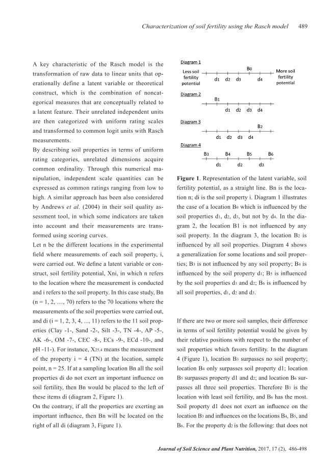
A key characteristic of the Rasch model is the transformation of raw data to linear units that op-erationally define a latent variable or theoretical construct, which is the combination of noncat-egorical measures that are conceptually related to a latent feature. Their unrelated independent units are then categorized with uniform rating scales and transformed to common logit units with Rasch measurements. By describing soil properties in terms of uniform rating categories, unrelated dimensions acquire common ordinality. Through this numerical ma-nipulation, independent scale quantities can be expressed as common ratings ranging from low to high. A similar approach has been also considered by Andrews et al. (2004) in their soil quality as-sessment tool, in which some indicators are taken into account and their measurements are trans-formed using scoring curves.Let n be the different locations in the experimental field where measurements of each soil property, i, were carried out. We define a latent variable or con-struct, soil fertility potential, Xni, in which n refers to the location where the measurement is conducted and i refers to the soil property. In this case study, Bn (n = 1, 2, …, 70) refers to the 70 locations where the measurements of the soil properties were carried out, and di (i = 1, 2, 3, 4, ..., 11) refers to the 11 soil prop-erties (Clay -1-, Sand -2-, Silt -3-, TN -4-, AP -5-, AK -6-, OM -7-, CEC -8-, ECs -9-, ECd -10-, and pH -11-). For instance, X25,4 means the measurement of the property i = 4 (TN) at the location, sample point, n = 25. If at a sampling location Bn all the soil properties di do not exert an important influence on soil fertility, then Bn would be placed to the left of these items di (diagram 2, Figure 1). On the contrary, if all the properties are exerting an important influence, then Bn will be located on the right of all di (diagram 3, Figure 1).

Figure 1. Representation of the latent variable, soil fertility potential, as a straight line. Bn is the loca-tion n; di is the soil property i. Diagram 1 illustrates the case of a location B0 which is influenced by the soil properties d1, d2, d3, but not by d4. In the dia-gram 2, the location B1 is not influenced by any soil property. In the diagram 3, the location B2 is influenced by all soil properties. Diagram 4 shows a generalization for some locations and soil proper-ties; B3 is not influenced by any soil property; B4 is influenced by the soil property d1; B5 is influenced by the soil properties d1 and d2; B6 is influenced by all soil properties, d1, d2 and d3.

If there are two or more soil samples, their difference in terms of soil fertility potential would be given by their relative positions with respect to the number of soil properties which favors fertility. In the diagram 4 (Figure 1), location B3 surpasses no soil property; location B4 only surpasses soil property d1; location B5 surpasses property d1 and d2; and location B6 sur-passes all three soil properties. Therefore B3 is the location with least soil fertility, and B6 has the most. Soil property d1 does not exert an influence on the location B3 and influences on the locations B4, B5, and B6. For the property d2 is the following: that does not


490 Moral et al.

influence on the locations B3 and B4, and influences on the locations B5 and B6. Finally, property d3 does not exert an influence on the locations B3, B4, and B5, and influences on the location B6. In this case, B6 is the location where soil fertility potential is greater since it is influenced by all the soil properties, d1, d2, and d3; B3 is the location where soil fertility potential is lower since it is not influenced by any property. On the other hand, d1 is the soil property which more fre-quently influences on soil fertility potential, and d3 is the soil property which less frequently influences on soil fertility potential. The probability that location n has the influence of the soil property corresponding to item i, given the pa-rameters Bn and di is:

which was obtained by Rasch (1980) in his treatise on latent variables. More information about the math-ematical formulation of the Rasch model can be ob-tained, for instance, in Ferrari and Salini (2011).In the literature, usually three variable selection tech-niques are utilized: spatial correlation analysis (e.g. Bazzi et al., 2013; Reich, 2008), principal component analysis (PCA) (e.g. Moral et al., 2010; Li et al., 2007), and multivariate spatial analysis based on Moran’s index PCA (MULTISPATI-PCA) (e.g., Gavioli et al., 2017; Córdoba et al., 2016; Peralta et al., 2015). PCA allows identifying a set of synthetic variables (princi-pal components) which are uncorrelated among them-selves and obtained from the original variables through some transformations. However, an important draw-back f PCA is that factors do not often have straightfor-ward interpretation. MULTISPATI-PCA adds a spatial restriction on the traditional PCA, introducing a spatial weighting matrix which is constructed using Moran’s bivariate spatial autocorrelation statistic. While in

PCA the spatial structures can exist in any component, in MULTISPATI-PCA the spatial structures are strong in the first components and, sometimes, its interpreta-tion is also difficult. In this sense, the Rasch model gives place to results which can be easily understood and there is no the necessity of defining any kind of weights; furthermore, original variables can be relat-ed or unrelated, that is, there are no initial constraints about the variables to be included in the model.In this work we aim to: (1) analyze the use of the Rasch model as a measurement tool to estimate with a rational basis the soil fertility potential, integrating many soil properties; (2) utilize the Rasch methodol-ogy to find out how each soil property have an influ-ence on the overall soil fertility; and (3) display any location which presents different behaviour with re-spect to the general fertility pattern.

2. Materials and Methods

The field research was carried out at a farm in the proximity of Badajoz (southwestern Spain). The area of the study site is 33 ha approximately. Gentle hills dominate the topography and, in the substrate, lime-stones predominate over intrusive acidic rocks. Ac-cording to the USDA-NRCS Soil Taxonomy System (1999), the soil is classified as Rhodoxeralf type.Soil samples were collected from the top layer, 0-20 cm, using a stratified random sampling scheme (Bur-rough and McDonnell, 1998) at 70 georeferenced places (Moral et al., 2011), and their coordinates were determined with a millimetric precision with a Maxor-GGDT differentially corrected global positioning sys-tem (Javad Navigation Systems, San Jose, California, USA). Soil samples were packed into plastic bags, air-dried and analyzed for particle-size distribution and other soil chemical properties (OM, pH, TN, AP, AK, CEC) using standard procedures (Moral et al., 2010). ECs and ECd data for all sampling sites were obtained



from kriged maps, which were generated from dif-ferent transects of the measurements of soil apparent electrical conductivity conducted using a 3100 Veris, a direct contact sensor (Moral et al., 2010).The formulation of the rating scale Rasch model was performed with the WINSTEPS v. 3.69 computer program (Linacre, 2009), which analyzes the com-plete data set, calculates fit statistics for each soil property item, and removes unnecessary items. As an output of this program, the empirical hierarchy of soil properties for predicting soil potential fertility, supporting by the considered data, is shown and re-lated to all soil samples, with each reported in logits, as well as any potential gaps in measure. Addition-ally, soil sample and property misfits are displayed.The formulation of the Rasch model to get a measure of soil fertility potential at each sample point, which would take into account the different contribution of 11 soil physical and chemical properties (clay, silt and sand content, ECd, ECs, OM, pH, TN, AP, AK, CEC), was achieved through different stages. Firstly, a previous transformation of the data to a common scale is necessary (Wright and Masters, 1982). Soil properties measures were categorically coded ac-cording to a plan where each sample was rated on a scale (1-5) for each soil property. Details of this process can be found in Moral et al. (2012).After including the categorical values in the data-base, these were processed by the WINSTEPS pro-gram. Previous to the development of all stages to analyze the model, it is important to denote that dur-ing the first study, considering all 11 soil properties, it was found that pH was not acceptable to support the latent variable; thus, it was eliminated and the program was rerun without this property. Later, the specific stage in which this fact was discovered will be displayed. So the following explanation is devot-ed to the analysis of the 10 remaining soil properties.

3. Results

From the program output, the beginning of a Rach analysis consists in studying whether the data fit the model reasonably. The overall information about how the data fit the model is contained in Table 1. According to Linacre (2009), fit statistics summarize the discrepancies between what has been observed and what was expected to be observed. They come in two different types: Infit and Outfit. Infit is an information-weighted or inlier-sensitive fit statistic that focuses on the overall performance of an item or subject. Outfit is an outlier-sensitive fit statistic that picks up rare events that have occurred in an unexpected way. They are the average of the squared standardized deviations of the observed performance from the expected performance, and a mean-square (MNSQ) fit statistic is a chi-square statistic divided by its degrees of freedom. Its expectation is 1.0. In this case, both Infit and Outfit MNSQ for soil sam-ples and properties are 0.99. Moreover, the mean standardized (ZSTD) Infit and Outfit, which are the sum of squares standardized residuals given as a Z-statistics (Edwards and Alcock, 2010), are expected to be 0, being in this study -0.1 for samples and -0.2 and -0.1 for items. Thus, on average, an overfit of the items is apparent, suggesting that the data fit the model better than expected, which could be possibly due to some redundant items. An index of the overall misfit for samples and items is the standard deviation of the Infit MNSQ (Bode and Wright, 1999). If 2 is an acceptable limit, both samples and items do not show important misfits because their values are 0.56 and 0.23 respectively; so, in this case, an acceptable overall fit of the data is evident. There is one statis-tics, the separation reliability, to estimate the inter-nal consistency of samples and items, i.e., the degree to which measures are free from error and therefore


492 Moral et al.

yield consistent results. Values close to 1 indicate a better reliability, considering values over 0.70 as ac-ceptable (Sekaran, 2000). For the data of the present

study, their values for samples and items are 0.81 and 0.94 respectively, which indicate a high consis-tency of data.

Table 1. Overall model fit information. Summary of all soil samples (70) and properties (10).

Total Score, sum of points of the common scale considering all soil properties; count, soil properties taken into account; measure,

logit position of the soil properties along the straight line that represents the latent variable, soil fertility potential; model error,

standard error of measurement; Infit and Outfit MNSQ, mean-square fit statistics to verify if items fit the model; Infit and Outfit

ZSTD, standardized fit statistics to verify if items fit the model.

The next step is to check how the assignment scale has been used. In Table 2 the step logit position, i.e., where a step marks the transition from one rating scale category to the next, is listed. From this Table 2, there are evidences to assert that the response scale was properly designed. Thus, the “Observed Average” increases by category value, the “Observed Average” values are similar to the “Sample Expected” ones, there is no misfit for any category because the Infit and Outfit MNSQ values are between 0.6 and 1.5 (Bode and Wright, 1999), and the “Structure Calibration” values increase with category. In consequence, for the data considered in this study, all categories have been used and are behaving according to expectation. After the previous analysis, it could be concluded that the rating scale categories are being used appropriately and the data reasonably fit the model.

Then, the following step is to analyze individual items to study their response to the model. Some suggestions for acceptable fit have been proposed in the literature (e.g., Bode and Wright, 1999), being the Infit and Out-fit MNSQ between 0.6 and 1.5, and the Infit and Outfit ZSTD between -3 and 2 the most usual. In this case study, all values are in the indicated intervals; in conse-quence, all considered soil properties support and have an important influence on soil fertility potential. As it was previously indicated, the analysis was initially performed using all 11 soil properties, including pH. However, in that case, the Infit and Outfit MNSQ, 2.24 and 2.38 respectively, fall outside the indicated range (0.6-1.5) for pH; moreover the Infit and Outfit ZSTD, 6.3 and 6.8, are also beyond the upper limit (2). Soil pH does not support the underlying latent variable for the considered data, so this property was eliminated and the analysis was rerun without it.



Table 2. Response scale use

Observed count, number of times the category was selected considering all samples and soil properties; observed average, mean

value of logit positions modelled in the category; sample expected, optimum values of the average logit positions for the data;

Infit and Outfit MNSQ, mean-square fit statistics to verify if items fit the model; structure calibration, logit calibrated difficulty

of the step representing the transition points between one category and the next.

One of the most important advantages of using the Rasch model is the possibility of the overall observa-tion, in the same scale, for all soil samples and their items or properties displayed in tandem. Thus, in Fig-ure 2 the relative distribution of the soil samples is provided in the upper half of the diagram according to the associated fertility potential, which have been achieved by means of all soil properties taken into ac-count, and, similarly, the soil properties are provided

in the lower half of the diagram, classified according to the fertility potential measure of the soil samples.Another complementary tool to display all samples according to their level of fertility potential is the Guttman scalogram (Linacre, 2009). As it can be seen in Table 3, soil samples are sorted descending by their level of fertility potential and soil properties are ar-ranged in the order indicated in the first row, so it en-ables to show their influence on each soil sample.

Figure 2. Soil samples and properties in the same scale. The straight line represents the latent variable: soil fertility potential. Distribution of soil samples (points) is above the line: to the right those more potentially fertile; to the left less those less potentially fertile. Soil properties are below the line: to the right less common (rare) properties, with lower influence on soil fertility; to the left more common (frequent) properties, with higher influence on soil fertility


494 Moral et al.

Table 3. Guttman scalogram for all soil properties (10) and samples (70). Only some sampling points, those with higher and lower fertility potential, are shown.

ECs, Soil Apparent Electrical Conductivity, 0-30 cm depth; ECd, Soil Apparent Electrical Conductivity, 0-90 cm depth; CEC,

Cation Exchange Capacity; TN, Total Nitrogen; OM, Organic Matter; AP, Available Phosphorus; AK, Available Potassium.

4. Discussion

After analyzing Figure 2, the soil property more to the right in the continuum, with the highest measure (0.96), is the AK. In consequence, it is the less com-mon soil property, i.e., it is the least frequently used to position the samples. On the contrary, to the left, both ECs and ECd are situated, and their measures are practically equal (-0.85 and -0.77 respectively). They are the more common soil properties, i.e., they are the most frequently used to position the samples. As both ECs and ECd are at the same position in the continuum, it could be possible to consider dropping one of them as redundant. In a similar way, CEC and clay content are located very close, so one of them could be also removed. Probably, this fact is due to the important relationship existing between both soil

properties (Moral et al., 2010). This result is consis-tent with the high values of Infit and Outfit, MNSQ and ZSTD, shown in Table 1, which also suggest this redundancy.A ranking of all considered soil properties has been obtained (Figure 2), indicating their influence on soil fertility in the experimental field. Thus, AK and AP are the properties with higher measure, exerting less influ-ence on soil fertility potential, and ECs and ECd the properties with lower measure, which have the greatest influence on soil fertility potential. If soil properties are grouped and the mean measure is determined, the most important properties are the ones making up soil appar-ent electrical conductivity (ECd and ECs), -0.81, fol-lowed by texture properties (sand, silt and clay content), -0.27, CEC, -0.17, OM, 0.53, and, finally, the primary nutrients (TN, AP, and AK), 0.69. This provides sup-



port for the usefulness and importance of ECd and ECs as indicators of soil fertility. The same results were ob-tained in the previous work, when both variables and texture were taking into account (Moral et al., 2012). ECa integrates the effects of various soil variables that govern soil fertility (Mertens et al., 2008) and, so, it seems logical that they are the main source of infor-mation about the overall nutritional condition in this soil. On the contrary, each individual primary nutrient does not contribute decisively to the overall soil fertil-ity potential. Of course, it does not mean primary nu-trient are not important for the crops, but if sufficient quantities are available in the soil, there is no need for increasing as they do not contribute to maximize the overall level of soil fertility potential.It is apparent that soil samples are quite homoge-neously distributed across the straight line (Figure 2). However, some of them, located to the left in the con-tinuum, have very low score, denoting their low fertil-ity potential. But, a majority of soil samples, located to the right, has adequate properties or propensity for inducing soil fertility potential. Soil samples can be also sorted according to their measure, displaying those which obtained higher value on the top. They are the most suitable locations for crops due to their higher fertility potential, while, on the contrary, those samples which got lower measure would be on the bottom, being potentially less fertile.With respect to the Guttman scalogram (Table 3), it has the advantage that a single variable is measured to analyze the individual behavior of each soil sample and, in the same way, study the individual pattern of each soil property. For example, sample 60, which is placed on top of the scalogram, has the highest scores for some soil properties (ECs, ECd, sand, CEC, TN, and AP); it has the higher soil fertility potential. If this sample is compared with sample 66, which also has the maximum total score but is the second in the ranking, it can be observed that they both have the maximum

score for ECs, ECd, sand, and TN; for the other soil properties, sample 60 has more highest scores (5). However, this sample has a low score in AK; possibly the soil fertility in this location could be improved if the amount of this nutrient is increased. The last in the Guttman scalogram is sample 11. It has low scores for all soil nutrients and all other soil properties, suggest-ing this location is the less favorable for any crop; it is the sample with lower soil fertility potential. Any other intermediate sample can be analyzed in a similar way, detecting the particular soil property in which a low value exists. In consequence, the Guttman sca-logram enables to systematize the data, being an ef-fective tool when an accurate selection of the most suitable areas for crops is desired, delimiting those zones where soil fertility potential is higher. More-over, comparisons between different soil samples, and consequently between different locations, and also site-specific amendments of any soil property with inadequate levels can be carried out.

5. Conclusions

The use of the Rasch measurement model in agro-nomic and soil issues, in this case study to estimate soil fertility potential, constitutes a new application of this method of great practical importance. In this work, particle-size distribution, ECa, CEC, pH, OM and the primary nutrients (N, P, and K) have been con-sidered as the influential variables on soil fertility and, after applying the Rasch methodology, a ranking of the soil samples according to their fertility potential and another one of soil properties according to their influence on soil fertility potential have been generat-ed. Previously, all stages to formulate the model were illustrated for 70 soil samples taken in an experimen-tal field. Thus, it was obtained that data fit the model very reasonably, yield consistent results and the as-signment scale with five categories was adequate.


496 Moral et al.

With regard to the delimitation of the latent variable soil fertility potential, the soil variables used in this case study are even in excess to properly classify the soil data; some of them could be eliminated because they are duplicated in the continuum. Thus, ECs or ECd could be alternatively chosen and, also, CEC or clay content. Moreover, the relative importance of the different soil properties that contribute to soil fertility potential is ascertained, being ECd and ECs the most important constituents of the latent variable soil fertil-ity potential, as they are indicators of several variables that govern soil fertility, followed by the textural frac-tions of soil, probably due to their capacity to regulate nutrients and water retention in the soil.In light of the results of the empirical analysis, some other conclusions can be drawn. Firstly, in the experi-mental area, a large number of soil samples have a high fertility potential, corresponding to the samples with higher Rasch measure. Nevertheless, there are some soil samples that do not reach an optimum fer-tility level, that is, their soil fertility potential is much lower than other neighbour locations, corresponding to the samples with lower Rasch measure. Secondly, the Guttman scalogram, where soil samples are sorted descending by their fertility potential and the influ-ence of each soil property is shown, is also a useful tool to find the more fertile locations and accomplish comparisons between them. Furthermore, places where any soil property has an inadequate level are easily found, which can be necessary to conduct site-specific treatments.In consequence, the proposed methodology allows us to discriminate, with a rational basis, locations in the experimental field where high soil fertility potential exists, integrating soil properties with different units, but all of them exerting an important influence on soil fertility. Considering spatial variability when making fertilizer management decisions can give place to bet-ter application of chemical substances, which leads to

a more cost-effective field management. Furthermore it can also improve environmental quality and crop-ping system sustainability.

Acknowledgements

The authors acknowledge financial support from the Junta de Extremadura (Project GR15050-Research Group TIC008, co-financed by European FEDER funds).

References

Álvarez, P. 2004. Transforming non categorical data for Rasch analysis. Rasch Measurement in health sciences. JAM Press. Maple Grove, Minnesota, USA.

Andrew, S.S., Karlen, D.L., Cambardella, C.A. 2004. The Soil Management Assessment Framework: a quantitative soil quality evaluation method. Soil Sci. Soc. Am. J. 68, 1945-1962.

Bazzi, C.I., Souza, E.G., Uribe-Opazo, M.A., Nó-brega, L.H.P., Rocha, D.M. 2013. Management zones definition using soil chemical and physical attributes in a soybean area. Engenharia Agrícola. 33, 952-964.

Bernardi, A.C.C., Bettiol, G.M., Ferreira, R.P., San-tos, K.E.L., Rabello, L.M., Inamasu, R.Y. 2016. Spatial variability of soil properties and yield of a grazed alfalfa pasture in Brazil. Precision Agric. 17, 737-752.

Bode, R.K., Wright, B.D. 1999. Rasch measurement in higher education. In: Smart, J.C., & Tierney, W.G. (Eds), Higher Education: Handbook of Theory and Research, vol. XIV. Agathon Press, New York.

Bond, T.G., Fox, C.M. 2007. Applying the Rasch Model: Fundamental Measurement in the Human Sciences (2nd Edition). Lawrence Erlbaum Asso-ciates Inc., Mahwah, NJ, USA.



Córdoba, M., Bruno, C., Costa, J.L., Peralta, N.R., Balzarini, M. 2016. Protocol for multivariate ho-mogeneous zone delineation in precision agricul-ture. Biosyst. Eng. 143, 95-107.

Corwin, D.L., Lesch, S.M. 2003. Application of soil electrical conductivity to precision agriculture: theory, principles and quidelines. Agron. J. 95(3), 455-471.

Edwards, A, Alcock, L. 2010. Using Rasch analysis to identify uncharacteristic responses to undergradu-ate assessments. Teaching Mathematics and Its Applications. 29, 165-75.

Ferrari, P.A., Salini, S. 2011. Complementary use of Rasch Models and Nonlinear Principal Compo-nent Analysis in the Assessment of the Opinion of European About Utilities. Journal of Classifica-tion. 28, 53-69.

Gavioli, A., Souza, E.G., Bazzi, C.L., Guedes, L.P.C., Schenatto, K. 2016. Optimization of management zone delineation by using spatial principal com-ponents. Comput. Electron. Agric. 127, 302-310.

Li, Y., Han, M.-Q., Lin, F., Ten, Y., Lin, J., Zhu, M.-Q., Guo, P., Weng, Y.-B., Chen, L.-S. 2015. Soil chemical properties, ‘Guanximiyou’ pummelo leaf mineral nutrient status and fruit quality in the southern region of Fujian province, China. J. Soil Sci. Plant Nutr. 15(3), 615-628.

Li, Y., Shi, Z., Li, F., Li, H.Y., 2007. Delineation of site-specific management zones using fuzzy clus-tering analysis in a coastal saline land. Comput. Electron. Agric. 56, 174-186.

Linacre, J.M. 2009. WINSTEPS (Version 3.69) [Computer Program]. John M. Linacre (Ed.). Chi-cago, USA.

Mertens, F.M., Pätzold, S., Welp, G. 2008. Spatial heterogeneity of soil properties and its mapping with apparent electrical conductivity. J. Plant Nutr. Soil Sci. 171, 146-154.

Moral, F.J., Rebollo, F.J., Terrón, J.M. 2012. Analysis of soil fertility and its anomalies using an objec-tive model. J. Plant Nutr. Soil Sci. 175, 912-919.

Moral, F.J., Terrón, J.M., Rebollo, F.J. 2011. Site-specific management zones based on the Rasch model and geostatistical techniques. Comp. Elec-tron. Agric. 75, 223–230.

Moral, F.J., Terrón, J.M., Marques da Silva, J.R. 2010. Delineation of management zones using mobile measurements of soil apparent electrical conduc-tivity and multivariate geostatistical techniques. Soil Till. Res. 106, 335-343.

Nájera, F., Tapia, Y., Baginsky, C., Figueroa, V., Ca-beza, R., Salazar, O. 2015. Evaluation of soil fer-tility and fertilisation practices for irrigated maize (Zea mays L.) under Mediterranean conditions in central Chile. J. Soil Sci. Plant Nutr. 15(1), 84-97.

Pedrera-Parrilla, A., Van De Vijver, E., Van Meir-venne, M., Espejo-Pérez, A.J., Giráldez, J.V., Vanderlinden, K. 2016. Apparent electrical con-ductivity measurements in an olive orchard under wet and dry soil conditions: significance for clay and soil water content mapping. Precision Agric. 17, 531-545.

Peralta, N.R., Costa, J.L., Franco, M.C., Balzarini, M. 2013. Delineation of management zones to improve nitrogen management of wheat. Comp. Electron. Agric. 110, 103–113.

Rasch, G. 1980. Probabilistic models for some intelli-gence and attainment tests. University of Chicago Press., 1960, Denmark. Revised and expanded ed.

Reich, R.M. 2008. Spatial Staistical Modelling of Natural Resources. Colorado State University. Fort Collins.

Serrano, J.M., Shahidian, S., Marques da Silva, J. 2016. Spatial variability and temporal stability of apparent soil electrical conductivity in a Mediter-ranean pasture. Precision Agric. In press.


498 Moral et al.

Sekaran, U. 2000. Research Methods for Business: A Skill Building Approach. John Wiley & Sons Inc., Singapore.

Tristán, A. 2002. Análisis de Rasch para todos. Ed. Ceneval. México.

Sudduth, K.A., Kitchen, N.R., Wiebold, W.J., Batch-elor, W.D., Bollero, G.A., Bullock, D.G., Clay, D.E., Palm, H.L., Pierce, F.J., Schuler, R.T., Thel-en, K.D. 2005. Relating apparent electrical con-ductivity top soil properties across the North-Cen-tral USA. Comp. Electron. Agric. 46, 263-283.

USDA-NRCS, 1999. Soil Taxonomy. A basic system of soil classification for making and interpreting soil surveys, 2nd ed. United States Department of Agriculture-Natural Resources Conservation Ser-vice, Washington, USA.

Wright, B.D., Masters, G.N. 1982. Rating scale analy-sis. MESA Press, Chicago.

characterization of soil fertility using the rasch model

Documents