CHARACTERIZATION OF SEDIMENTS FROM TUNGABHADRA RESERVOIR FOR SUSTAINABLE

DEVELOPMENT

PROJECT REFERENCE NO.: 38S1571

COLLEGE : NEW HORIZON COLLEGE OF ENGINEERING, BANGALORE

BRANCH : CIVIL ENGINEERING

GUIDE : MR. CHANNABASVARAJ W

STUDENTS : MR. HARISH KUMAR.C

MR. RAMU P

MR. JEEVAN KUMAR

MR. SANTOSH NYAMAGOUD

Introduction:

The Tungabhadra Dam is constructed across the Tungabhadra River, a tributary

of the Krishna River. The dam is near the town of Hospet in Karnataka. It is a

multipurpose dam serving irrigation, electricity generation, flood control, etc. This is a

joint project of erstwhile Hyderabad state and erstwhile Madras Presidency when the

construction was started; later it became a joint project of Karnataka and Andhra

Pradesh after its completion in 1953. The main architect of the dam was

Dr.ThirumalaiIyengar, an engineer from Madras.

The dam creates the biggest reservoir on the Tungabhadra River with 101 thousand

million cubic feet (TMC) of gross storage capacity at full reservoir level (FRL) 498 m

MSL, and a water spread area of 378 square kilometres. The dam is 49.5 meters high

above its deepest foundation. The left canals emanating from the reservoir supplies water

for irrigation entirely in Karnataka state. Two right bank canals are constructed one at low

level and the other at high level serving irrigation in Karnataka and Rayalaseema region of

Andhra Pradesh. Hydropower units are installed on canal drops. The reservoir water is

used to supply water to downstream barrages Rajolibanda and Sunkesula located on

the Tungabhadra River. The identified water use from the project is 230 tmcft by

the Krishna Water Disputes Tribunal. Karnataka and Andhra Pradesh got 151 tmcft and 79

tmcft water use entitlement respectively.

On the right side of the dam, Sanduru hill ranges extending up to 800 m MSL are

close to the periphery of the Tungabhadra reservoir. These hill ranges from the Sanduru

valley located above 600 m MSL. This reservoir is an ideal place to install pumped

storage hydropower plants and lift irrigation projects. A moderate high level storage

reservoir of capacity 20 tmcft at FRL 620 m MSL, can be constructed by damming the

Sanduru valley. This reservoir will serve as upper pond and existing Tungabhadra

reservoir as tail pond for installing pumped-storage hydroelectricity units. The water

pumped during the monsoon months into the upper pond can be diverted by gravity to

irrigate an extensive area in the uplands up to 600m MSL in Rayalaseema and Karnataka.

This water can be pumped further To plan

for future requirements and improvements of road in view of anticipated

developments.

To work out financing systems to meet the drinking water requirements of 5 districts.

However, the available water resources at Tungabhadra dam are over-used, and water

shortages are frequent. Water availability in the reservoir could be augmented by

transferring water from the Krishna River, if a link canal were constructed from

the Almatti / Narayanpur reservoir to the Tungabhadra reservoir.

This canal would supply Krishna River water to the existing right bank canal of

Tungabhadra dam and would augment water in Tungabhadra reservoir. Envisaging small

balancing reservoirs where this link canal is intercepting the tributaries of Tungabhadra

River would facilitate water diversion to Tungabhadra reservoir for augmenting further

water availability. When this joint project of Karnataka and Andhra Pradesh is

constructed, nearly 400 tmcft water additionally will be available for irrigation and

drinking purposes in the high drought risk uplands of Rayalaseema and Karnataka.

Excavation of sediments from the bed of sea, rivers, lakes, reservoirs, ponds and

lagoons is termed as dredging. It is usually executed to create, and maintain, navigable

waterways/channels. It also deals with removal of the polluting toxicants from the water

bodies and hence their cleaning, which helps in preserving the marine ecosystem.

Dredging results in huge quantity of the dredged material (sediments) which requires a

special attention as far as its handling, disposal and usage for infrastructure development

is concerned. It is worth noticing that the type (read characteristics) of the dredged

material will greatly influence the method of its disposal. However, the environmental

regulations restrict open water disposal of the dredged material and warrant alternative

methods of its utilization. In this context, one of the potential applications of the dredged

material is its utilization for reclaiming the land, which is better known as “reclamation”.

Owing to shortage of the land for catering to the increasing demand for housing,

transportation as well as commercial and industrial activities, due to rise in human

population, reclaiming land from the sea has become a welcome exercise.

Furthermore, though, in the past, hill-cut materials, seabed sand, and other locally

available materials such as gravels have been used as the fill material for land

reclamation, their scarcity and transportation from the far off sites becomes a major issue.

However, utilization of the sediments from dredging mainly depends on their physical

characteristics (viz., sands, silts, clay, and moisture retention), chemical characteristics

(viz., organic and inorganic contents, and the extent of toxicity), engineering

characteristics (viz., sedimentation, strength and compressibility) and vulnerability

towards microbial degradation. This calls for development of a comprehensive

characterization protocol for establishing the suitability of the dredged material for its

beneficial usages (viz., land reclamation, agricultural fill, etc.). This necessitates complete

characterization of the sediments.

In order to effectively utilize the sediments (predominantly containing silt and clay)

for land reclamation, suitable dewatering techniques need to be developed for

accelerating consolidation and hence their strengthening. In this context, various

techniques such as pre- loading, vacuum consolidation, application of prefabricated

vertical drains and geotubes, have been used in the past. However, these techniques have

their own limitations and are quite cost intensive. As such, efforts should be made to

stabilize the sediments by using thermal heat flux and appropriate admixtures (viz.,

construction debris and slag based micro-fine cement), which do not contain carbon rich

compounds that could affect the environment. Furthermore, as the efficiency of the

dredging process would impact the cost of dredging, which in turn would influence the

economics of the reclamation process, establishing “Dredgeability Index”, which relates

characteristics of the material to be dredged and the dredging equipment to be used,

would be quite prudent. This index will be an excellent guiding tool for selection of

proper dredging equipment for dredging operations.

Objectives: The objectives of this project work is to: • Physical characterization of sediments from Tungabhadra reservoir. - Particle size distribution test - sedimentation test - specific gravity determination - plasticity determination - organic content determination • Chemical characterization of sediments from Tungabhadra reservoir. - Presence of minerals in the sediments - Morphological properties of sediments are also studied - Geotechnical properties of the sediments determined Experimental work:

Determination of moisture content by oven drying method

Determination of moisture content by oven drying method of the sample were determined

by conducting the experiment, as per IS:2720 (PART-2)-1973 Soil particles having a porous

structure, the pores (voids) may have water or air. If voids are fully filled with water, the soil

is called saturated soil and if voids have only air, it is called dry soil.

Moisture content is defined as the ratio of the mass or weight of water to the mass or

weight of soil solids expressed as percentage.

w = Ww

Ws × 100

Where;

w = moisture content

Ww = mass or weight of water contained in the voids

Ws = mass or weight of soil solids (mass of oven dry soil)

For moisture content determination, the soil samples are dried to a temperature at which only pore water is evaporated. The standard temperature for oven drying of normal soil is 105°C to 110°C

Specific gravity

The specific gravity, Gs, of the sample was determined by using Pychnometer method, as per IS:2720 (PART-3)-1980. Clean, dry and weigh the pycnometer along with the lid accurately. Let the weight be W1.Take about 200 g of oven dried soil sample (passing through 4.75 mm IS sieve) in the pycnometer and weigh it along with the lid. Let this weight be W2. Add distilled water to the soil in pycnometer (while stirring with a glass rod to remove the entrapped air) to cover the remaining part of the pycnometer up to an already marked level/ top of the cap. Then note down its weight as W3. Empty the pycnometer and clean it. Fill the pycnometer with distilled water upto the same level as in step 3. Note down its weight as W4 as shown in Fig.5.4. Conduct two more trials of the test, and note the average of the three values as the specific gravity of the soil sample. Average of three values of the same soil sample is taken and reported to the nearest 0.01

Gradational characteristic

The particle-size distribution characteristics of the sample were determined by conducting the sieve analysis, as per IS:2720 (PART-4)-1985

Liquid limit test

Liquid limit of the soils were determined according to the guidelines of IS:9259-1979.

Adjust the cup of the liquid limit apparatus with the help of grooving tool gauge and the

adjustment plate to give a drop of exactly 1 cm on the point of contact on base. Weigh

about 120 g of air-dried soil passing 425μ I.S sieve. Mix it thoroughly with some distilled

water to from a uniform paste. Place a portion of the paste in the cup of the liquid limit

device; smooth the surface with spatula to a maximum depth of 1cm. Draw the grooving

tool through the sample along the symmetrical axis of the cup, holding the tool

perpendicular to the cup. Turn the handle at a rate of 2 revolutions per second and count

blows until two parts of the soil sample come into contact at the bottom of the groove

along a distance of 10mm.Transfer about 15g of the soil forming the edges of the groove

that flowed together to a water content tin and determine the water content by oven

drying. Transfer the remaining soil in the cup to the main soil sample in the basin and mix

thoroughly after adding a small amount of waste.

Plastic limit test

Plastic limit of the soils were determined according to the guidelines of IS:9259-1979. Take

about 30g of air dried sample passing through 425μ I.S sieve. Mix it thoroughly with distilled

water in the evaporating dish till the soil mass becomes plastic enough to be easily molded

with fingers. Take about 10g of this plastic soil mass and roll it between fingers and glass

plate with just pressure to roll the mass into a thread of uniform diameter throughout its

length. The rate of rolling shall be between 60 and 90 strokes per minute. Continue rolling till

you get a thread of 3 mm diameter. If the 3mm thread doesn’t crack, it shows that the water

content is more than the plastic limit. Kneed the soil together to a uniform mass and re-roll.

Continue the process until the thread crumbles when the diameter is 3 mm. Collect the pieces

of the crumbled thread in air tight container for moisture content determination. Repeat the

test to at least 3 times and take the average of the results calculated to the nearest whole

number.

Shrinkage limit test

Shrinkage limit of the soils were determined according to the guidelines of IS:9259-1979.

Mix about 30gm of soil passing 425μ I.S sieve with distilled water. The water added should

be sufficient to make the soil past enough to be readily worked into the shrinkage dish

without inclusion of air bubbles.

Coat the inside of two shrinkage dish with a thin layer of Vaseline. Place the soil sample in

the dish, by giving gentle taps. Strike off the top surface with a straight edge. Weigh the

shrinkage dish immediately full of wet soil. Dry the dish fist in air and then in oven. Weight

the shrinkage dish with dry soil pat.

Clean and dry the shrinkage dish and determine its empty mass. Also weigh an empty

porcelain dish (small size) which will be used for weighing dish. Keep the shrinkage dish in a

large porcelain dish, fill it to overflowing with mercury and remove the excess by pressing

the plate firmly over the top of the dish. Transfer the contents of the shrinkage dish to the

mercury weighing dish and weight. Place the glass cup in a large dish. Fill it to over flowing

with mercury; remove the excess by pressing the glass plate with three prongs firmly over the

top of the cup.

Consistency limits

Consistency limits (Liquid limit, WL, Plastic limit, WP) of the soils were determined

according to the guidelines of IS: 9259-1979.

Free swell index

Free swell index, FSI, of the soils were determined according to guidelines of IS:

2720 (Part-40) 1977. Where two 10 grams soil specimens were taken which is oven dry

passing through 425-micron IS sieve. Each soil specimen shall be poured in each of the two

glass graduated cylinders of 100ml capacity. One cylinder shall then be filled with kerosene

oil and the other with distilled water up to the 100ml mark. After removal of entrapped air the

soils in both the cylinders shall be allowed to settle. Sufficient time (not less than 24 hours)

shall be allowed for the soil sample to attain equilibrium state of volume without any further

change in the volume of the soils. The final volume of soils in each of the cylinders shall be

read out. By employing Eq. 5.1, FSI of the sample (in m2/g) was determined and the results

are presented in Table 5.1. It has been observed that the FSI for sediments SS-1 and SS-2 are

zero has these soils contains very less amount of fines (clay percentage) and sediments SS-3

and SS-4 also exhibits Very less swelling (1%). Though the amount of clay present in these

sediments is around 13 to 17% but this clay is inactive and hence swelling is very less.

Free swell index, percent= 𝑉𝑉𝑑𝑑−𝑉𝑉𝑘𝑘𝑉𝑉𝑘𝑘

𝑋𝑋 100 (5.1)

Where,

Vd =The final volume of soil in distilled water

Vk = The final volume of soil in kerosene

Hydrometer analysis

Hydrometer analysis is a widely used method of obtaining an estimate of the

distribution of soil particle sizes from the No. 200 (0.075 mm) sieve to around 0.01 mm. The

data are presented on a semi log plot of per cent finer vs. particle diameters and may be

combined with the data from a sieve analysis of the material retained (+) on the No.200 sieve.

The principal value of the hydrometer analysis appears to be to obtain the clay fraction

(generally accepted as the per cent finer than 0.002 mm). The hydrometer analysis may also

have value in identifying particle sizes < 0.02 mm in frost susceptibility checks for pavement

subgrades. This test is done when more than 20% pass through No.200 sieve and 90% or

more passes the No. 4 (4.75 mm) sieve.

Mix 100 ml of the 5% dispersing solution and 880 ml of demonized water in a 1000

ml cylinder. This mixture is the blank. (Note: 100 ml + 880 ml = 980 ml. This blank is not

diluted to 1000 ml; the other 20 ml is the volume occupied by 50 g of soil.). Weigh 25-50 g

of soil and transfer r to a dispersing cup. Record weight to ± 0.01g. Add 100-ml of 5%

dispersing solution. Attach dispersing cup to mixer and mix the sample for 30 – 60 sec.

Transfer the suspension quantitatively from the dispersing cup to a 1000 ml cylinder. Fill to

the 1000-ml mark with deionized water equilibrated to room temperature, or allow to stand

overnight to equilibrate. At the beginning of each set, record the temperature, and the

hydrometer reading of the blank, using the procedure described below. To determine the

density insert plunger into suspension, and carefully mix for 30 sec. until a uniform

suspension is obtained. Remove plunger (begin 40 second timer) and gently insert the

hydrometer into the suspension. Record the hydrometer reading at 40 sec. This is the amount

of silt plus clay suspended. The sand has settled to the bottom of the cylinder by this time.

Record the hydrometer reading again after 6 hours, 52 minutes. This is the amount of clay in

suspension. The silt has settled to the bottom of the cylinder by this time.

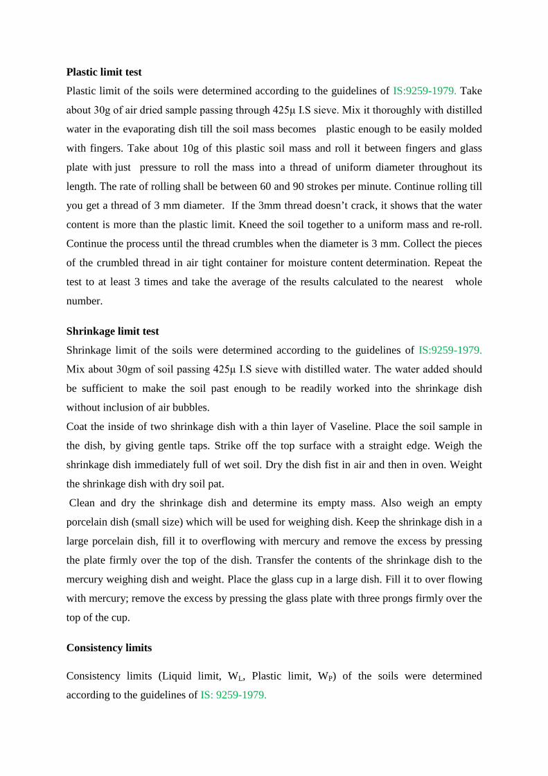
Compaction characteristics

Compaction characteristics, of the soils were determined according to guidelines of IS:

10074-1982. The compaction characteristics of the three soil samples (viz., SS-1, SS-2, SS-3

and SS-4) were established by employing compaction device as per IS 2720. The apparatus

consists of a cylindrical mould of 100 mm internal diameter, 127.3 mm in height and

standard compaction energy can be achieved. The results obtained from the compaction test

(viz., optimum moisture content and maximum dry density) are listed in the Table.5.2. Also

compaction curve for different soils are presented in Figure.5.13. It is observed from the

results that the three soils exhibits very good range of MDD and OMC with respect to

backfill material (for highways and any reclamation activities) and hence these soils are best

suited for backfill purpose as for as strength criteria.

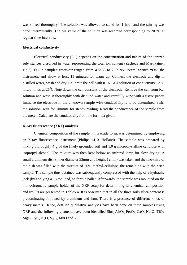
Unconfined compression test

Unconfined compression test of the soils were determined according to the guidelines of IS-

4332 (Part-5)1970, soil is put in the mould of diameter 38mm and height 76mm, and

compressed to size. The specimen is extracted carefully. Measure the initial length and

diameter of the specimen. Place the specimen on the lower plate and raise it to make contact

with the upper plate. Adjust the compression dial gauge and proving ring to read zero Apply

the compression load to produce an axial strain at the rate of 0.5 to 1 % per minute. Record

the readings of dial gauge and proving ring. Continue the compression till the specimen fails

or 20% vertical deformation is reached whichever occurs earlier. Sketch the failure pattern

and measure the failure angle with the horizontal if possible.

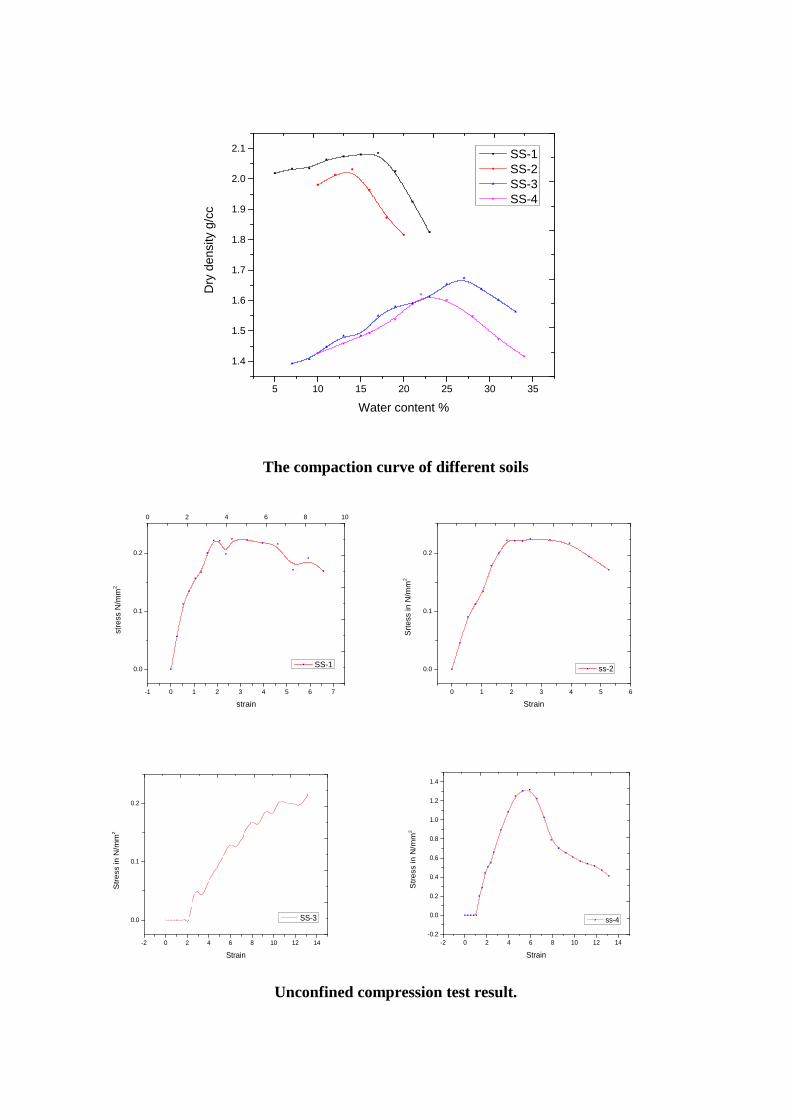
California bearing ratio test

CBR value as defined by IS: 2720 (Part-14) - 1979 is the ratio of the force per unit

area required to penetrate a soil mass with a circular plunger of 50mm diameter at the rate of

1.25 mm per minute, penetration of a standard material. The material was sieved through 20

mm IS sieve. 5 kg of sample was taken and water was added to the soil in such a way that the

moisture content of the specimen was either equal to field moisture content or optimum

moisture content as desired. Then it was mixed thoroughly and uniformly. The mould was

clamped along with the extension collar to the base plate. The coarse filter paper was placed

on the perforated base plate. The mould containing compacted soil was inverted and it was

then clamped to the base plate. The soil was filled in the mould in 5 layers; each layer was

compacted by 56 blows with the rammer weighing 4.89 kg dropping through 450mm. The

mould containing the specimen was placed on the testing machine. An annular weight of

2.5kg was placed on the top surface of the soil. The penetration plunger was made to come

into contact with soil surface and a load of 4 kg was applied so that full contact between soil

and plunger was established. The remainder surcharge weight was placed so that the total

surcharge weight equals to 5 kg. The dial gauge readings were set to zero. The load was

applied so that the penetration rate was 1.25 mm per minute. The load at penetrations of 0.5,

1, 1.5, 2, 2.5, 3, 4, 5, 7.5,10, and 12.5 mm were recorded. Plot the Load- Penetration curve

with load as ordinate and penetration as abscissa. Sometimes the initial portion of the curve is

concave upwards due to surface irregularities. In such a case, draw tangent at the point of

greatest slope. The point where this tangent meets the abscissa is the corrected zero-reading

of penetration.

CBR Value =test load corresponding to chosen penetration standard load for the same penetration

x 100 %

The CBR value at 2.5 mm penetration will be greater than that at 5mm and in such a case; the

former is taken for design purpose. If 5 mm value is greater, the test is repeated. If the same

results follow, the CBR value corresponding to 5 mm penetration is adopted for design

purposes. The result obtained from the test are listed in table.5.2, also Figure:-5.17shows the

variation of load at different penetration.

Chloride test

Chloride test of the soils were determined according to the guidelines of IS-2720

(Part-24)1976, Chloride ions are generally present in natural waters in the form of salts of

sodium, potassium and calcium. The main sources of chlorides in reservoir are the dissolution

of salt deposits, discharges of effluents from industries, sewage dis- charges, irrigation, etc.

The values were within the permissible limit of 1000mg/l. Pipette out 50ml of the given water

sample into clean conical flask. Add 3 drops of Potassium chromate indicator. The solution

turns yellow in colour. Titrate this with 0.0141 N AgNO3 to a stable reddish brown or brick

red precipitate.

Total Hardness

Total Hardness test of the soils were determined according to the guidelines of IS-

2720 (Part-24)1976, Hardness primarily due to the presence of calcium and magnesium ions

measures the capacity of water to precipitate soap. Some cat- ions (like iron, strontium and

manganese) and anions (such as carbonates, bicarbonates, sulphate, chloride, nitrate and

silicates) contribute to hardness in aquatic ecosystems (APHA 2005). The degree of hardness

of drinking water has been classified (WHO 2004) in terms of its equivalent CaCO3

concentration. Pipette out 50ml of the given water sample into a conical flask. Add 1ml of

ammonia buffer solution and 3 drops of Erichrome black-T indicator to it. The solution turns

wine red in color. Titrate this solution against 0.01 M EDTA taken in a burette till the color

changes from wine red to blue which indicates the end point. Note down this burette reading

which gives the volume of EDTA consumed.

Permanent Hardness

Permanent Hardness test of the soils were determined according to the guidelines of IS-2720

(Part-24)1976, Permanent hardness is caused due to the presence of sulphates, chlorides and

nitrates of calcium and magnesium. This cannot be removed by boiling but requires special

treatment such as demineralization, ion exchange etc. Take about 60 ml of the given water

sample, boil and cool (to remove temporary hardness) and transfer 50 ml of this solution into

a clean conical flask. Add 1ml of ammonia buffer solution and 3 drops of Erichrome black-T

indicator to it. The solution turns wine red in colour. Titrate this solution against 0.01 M

EDTA taken in a burette till the colour changes from wine red to blue which indicates the end

point. Note down this burette reading which gives the volume of EDTA consumed.

Alkalinity

Alkalinity test of the soils were determined according to the guidelines of IS-2720

(Part-24)1976, Alkalinity is a measure of the ability of water to neutralize acids. It is due to

the presence of bicarbonates, carbonates and hydroxide of calcium, magnesium, sodium,

potassium and salts of weak acids and strong bases as borates, silicates, phosphates, etc.

(APHA 2005). Large amount of alkalinity imparts a bitter taste, harmful for irrigation as it

damages soil and hence reduces crop yields.

Take 50ml of sample (Water) in a conical flask, add 2-3 drops of Methyl orange

indicator. Titrate the contents in the conical flask with 0.02N H2SO4. The end point is pale

yellow to pale pink. Note the burette reading, which gives the volume of H2SO4. Repeat till

two concurrent values are obtained.

Acidity

Acidity test of the soils were determined according to the guidelines of IS-2720 (Part-

24)1976, Acidity of a solution is a measure of its capacity to neutralize bases. Acidity is

caused due to the presence of mineral acids (E.g. Al2(SO4)3, Fe2SO4), CO2, strong acids and

weak bases. This is caused mainly due to industrial wastes. Acidity of a sample is determined

by titrating against a strong solution of a base (alkali) such as NaOH. Pipette out 50ml of the

given water sample into a clean conical flask. Add 3 drops of phenolphthalein indicator to it.

The solution becomes colourless. Titrate this solution against 0.02 N NaOH solution taken in

the burette till the colour changes to pink. Note down the burette reading which indicates the

volume of NaOH run down (consumed). Repeat the experiment until at least 2 concurrent

readings are obtained.

pH Value Test

pH of water changes with time due to expo- sure to air, variation in temperature and

due to biological activities. pH is governed by the equilibrium between carbon dioxide,

carbonate and bicarbonate ions. The pH of the sample was determined as per IS-2720 (Part-

26)-1987, by using a digital pH meter (Elico Private Ltd. Make, Model L1-120). The pH was

established corresponding to liquid to solid ratio, L/S, varying between 2 and 20. The pH

meter was calibrated by using different standard buffer solutions (pH=4, 7 and 9.2) prior to

each measurement. 30 g sample was mixed with distilled water and the resultant suspension

was stirred thoroughly. The solution was allowed to stand for 1 hour and the stirring was

done intermittently. The pH value of the solution was recorded corresponding to 20 °C at

regular time intervals.

Electrical conductivity

Electrical conductivity (EC) depends on the concentration and nature of the ionized

sub- stances dissolved in water representing the total ion content (Zacheus and Martikainen

1997). EC in sampled reservoir ranged from 472.88 to 2589.95 µS/cm. Switch “On” the

instrument and allow at least 15 minutes for warm up. Connect the electrode and dip in

distilled water, wash and dry. Calibrate the cell with 0.1N KCl solution of conductivity 12.89

micro mhos at 250C.Note down the cell constant of the electrode. Remove the cell from Kcl

solution and wash it thoroughly with distilled water and carefully wipe with a tissue paper.

Immerse the electrode in the unknown sample wise conductivity is to be determined, swirl

the solution, wait for 1minute for steady reading. Read the conductance of the sample from

the meter. Calculate the conductivity from the formula given.

X-ray fluorescence (XRF) analysis

Chemical composition of the sample, in its oxide form, was determined by employing

an X-ray fluorescence instrument (Philips 1410, Holland). The sample was prepared by

mixing thoroughly 4 g of the finely grounded soil and 1.0 g microcrystalline cellulose with

isopropyl alcohol. The mixture was then kept below an infrared lamp for slow drying. A

small aluminum dish (inner diameter 33mm and height 12mm) was taken and the two-third of

the dish was filled with the mixture of 70% methyl-cellulose, the remaining with the dried

sample. The sample thus obtained was subsequently compressed with the help of a hydraulic

jack (by applying a 15 ton load) to form a pallet. Afterwards, the sample was mounted on the

monochromatic sample holder of the XRF setup for determining its chemical composition

and results are presented in Table5.4. It is observed that in all the three soils silica content is

predominating followed by aluminum and iron. There is a presence of different kinds of

heavy metals. Hence, detailed qualitative analyses have been done on these samples using

XRF and the following elements have been identified Sio2, Al2O3, Fe2O3, CaO, Na2O, TiO2,

MgO, P2O5, K2O, V2O5, MnO and V.

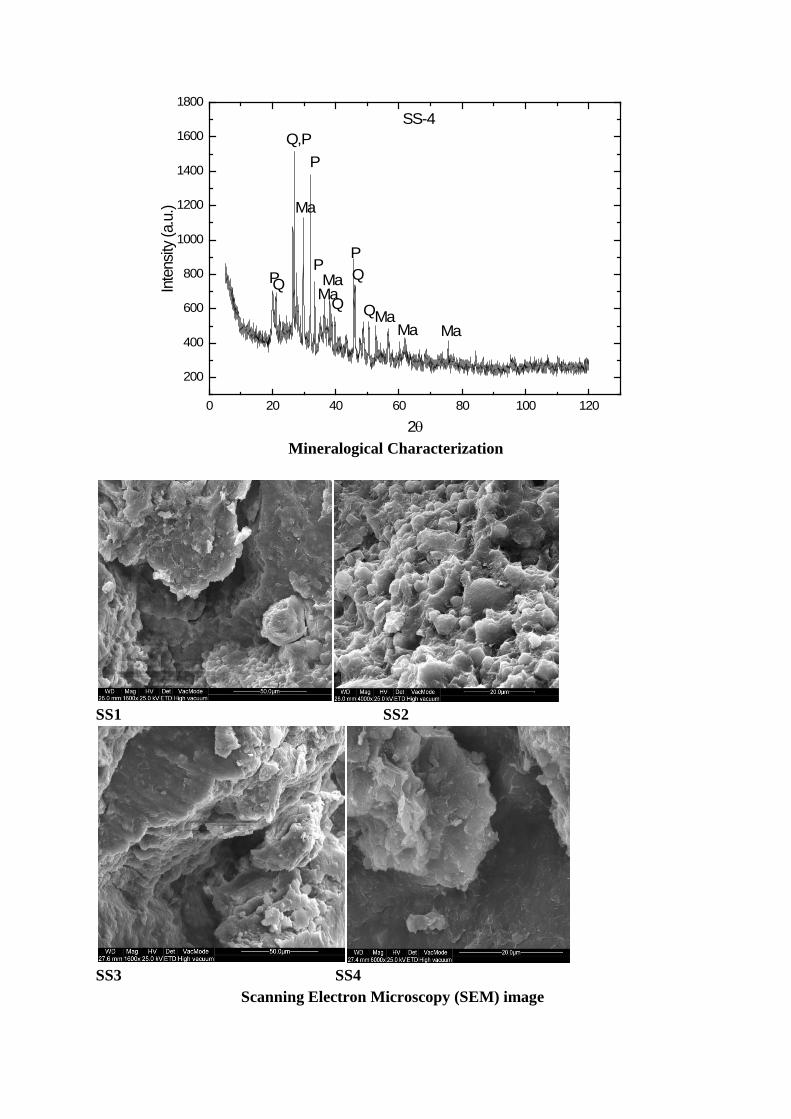
Scanning Electron Microscopy (SEM)

In order to distinguish the environmental characteristics of the sediments and to categorize the various surface features of the sediments, scanning electron micrographs of the sediment samples were obtained by employing Quanta make 200 ESEM.

RESULTS AND DISCUSSIONS:

Table:-5.1 Physical Analysis.

1E-3 0.01 0.1 1

0

20

40

60

80

100

% F

INER

GRAIN SIZE

SS-1 SS-2 SS-3 SS-4

1E-3 0.01 0.1 1

0

20

40

60

80

100

Grain size distribution.

Designation

% Fraction WC (%) G

OC

(%)

Atterberg Limits (%)

SL FSI USCS

Sand Silt Clay LL PL PI

SS-1 84 15 1 14 3.47 2.6 Non-plastic 0 0 SM

SS-2 86 13 1 22 3.37 3.1 Non-plastic 0 0 SM

SS-3 66 21 13 47 2.38 6.2 43 38 5 28 2 SM

SS-4 64 19 17 51 2.49 6.4 38 29 9 26 1 SM

5 10 15 20 25 30 35

1.4

1.5

1.6

1.7

1.8

1.9

2.0

2.1

Dry

den

sity

g/c

c

Water content %

SS-1 SS-2 SS-3 SS-4

The compaction curve of different soils

-1 0 1 2 3 4 5 6 7

0.0

0.1

0.2

stre

ss N

/mm

2

strain

SS-1

0 2 4 6 8 10

0 1 2 3 4 5 6

0.0

0.1

0.2

Srte

ss in

N/m

m2

Strain

ss-2

-2 0 2 4 6 8 10 12 14

0.0

0.1

0.2

Stre

ss in

N/m

m2

Strain

SS-3

-2 0 2 4 6 8 10 12 14-0.2

0.0

0.2

0.4

0.6

0.8

1.0

1.2

1.4

Stre

ss in

N/m

m2

Strain

ss-4

Unconfined compression test result.

0 2 4 6 8 10 12 14

0

10

20

30

40

50

60

LOAD

IN K

G

PENETRATION N MM

SS-1

0 2 4 6 8 10 12 14

0

50

100

LOAD

IN K

G

PENTRATION

SS-2

0 2 4 6 8 10 12 14

1

2

3

4

5

6

LOAD

IN K

G

PENETRATION IN MM

SS-3

0 2 4 6 8 10 12 14

2

4

6

LOA

D IN

KG

PENETRATION IN MM

SS-4

California bearing ratio test result

SL.No Sample no.

MDD kN/m3

OMC (%)

UCS Kg/cm2

Cohesion kN

CBR in

(%)

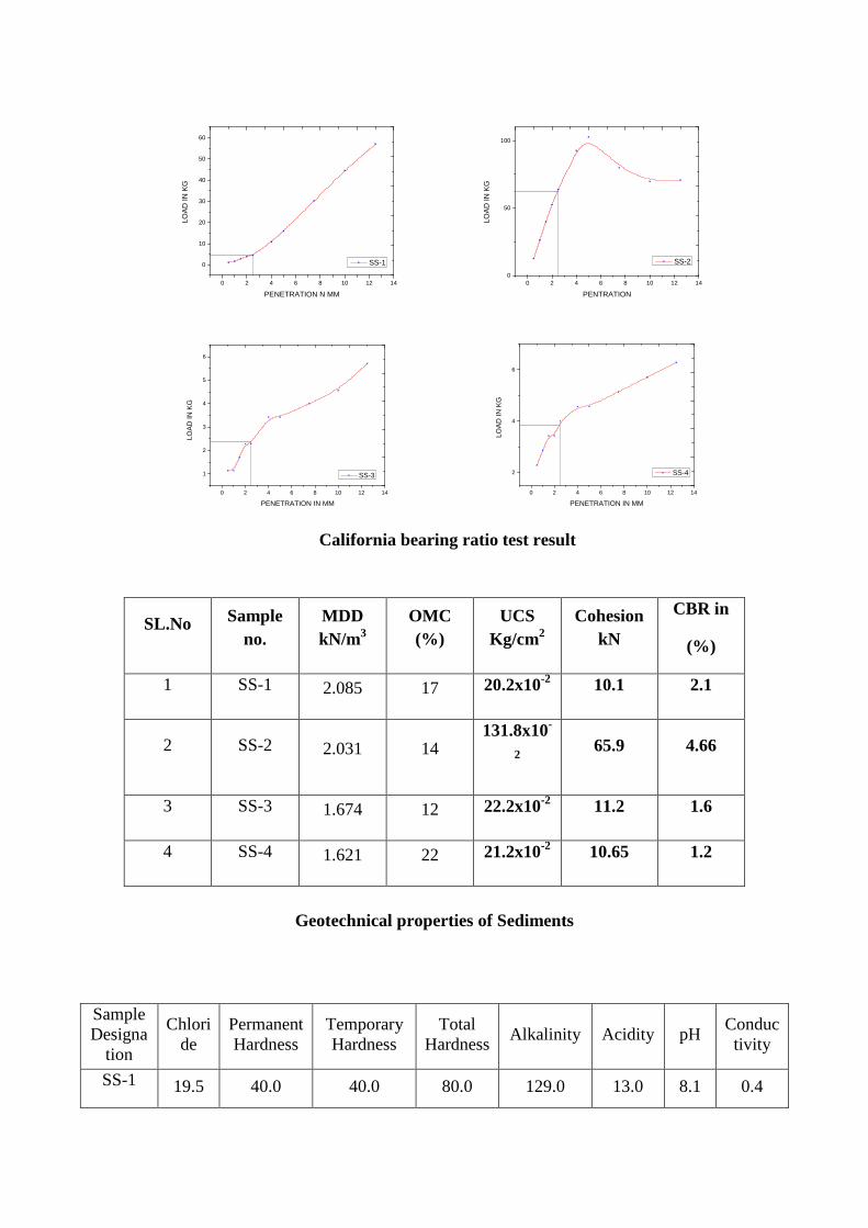
1 SS-1 2.085 17 20.2x10-2 10.1 2.1

2 SS-2 2.031 14 131.8x10-

2 65.9 4.66

3 SS-3 1.674 12 22.2x10-2 11.2 1.6

4 SS-4 1.621 22 21.2x10-2 10.65 1.2

Geotechnical properties of Sediments

Sample Designa

tion

Chloride

Permanent Hardness

Temporary Hardness

Total Hardness Alkalinity Acidity pH Conduc

tivity

SS-1 19.5 40.0 40.0 80.0 129.0 13.0 8.1 0.4

SS-2 20.5 35.0 6.0 41.0 120.0 09.0 7.9 0.3

SS-3 134.5 162.0 98.0 260.0 186.0 29.0 7.5 0.4

SS-4 29.0 86.0 0.0 106.0 368.0 26.0 8.3 0.3

Chemical composition of different soil samples

Designation Sio2 Al2O3 Fe2O3 CaO Na2O TiO2 MgO P2O5 K2O V2O5 MnO

SS-1 15.9 17.9 43.8 13.0 4.1 2.0 1.6 0.8 0.6 0.1 0.1

SS-2 14.3

15.8 44.5 9.8 9.7 2.2 1.9 0.7 0.8 0.1 0.1

SS-3 19.2

12.0 14.5 11.2 36.5 2.3 2.3 0.9 0.8 0.1 0.1

SS-4 13.1 40.8 39.0 0.2 0.6 2.4 0.7 0.8 0.8 0.1 1.3

X-ray fluorescence (XRF) analysis

0 20 40 60 80 100 120200

400

600

800

1000

1200

1400

1600

1800

2000

2200

Inte

nsity

(a.u

.)

2θ

SS-1

I,Q

MuI,M

Q,I Mu,MI,M

0 20 40 60 80 100 120200

400

600

800

1000

1200

1400

1600

1800

2000

2200

Inte

nsity

(a.u

.)

2θ

SS-1

I,Q

MuI,M

Q,I Mu,MI,M

0 20 40 60 80 100 120200

400

600

800

1000

1200

1400

1600

1800

2000

2200

Inte

nsity

(a.u

.)

2θ

SS-2

I,Q

MuI,M

Q,I Mu,MI,M

0 20 40 60 80 100 120200

400

600

800

1000

1200

1400

1600

1800

SS-3

Inte

nsity

(a.u

.)

2θ

I,EQ

Q,I

EEI,E

I,EI,Q Q

0 20 40 60 80 100 120

200

400

600

800

1000

1200

1400

1600

1800

SS-4

Inte

nsity

(a.u

.)

2θ

PQ

Q,P

Ma

Ma

Q

QMaQ

MaMa

P

PP

Ma

Mineralogical Characterization

SS1 SS2

SS3 SS4

Scanning Electron Microscopy (SEM) image

CONCLUSION:

• Objective of this present study is to increase the storage capacity of reservoir and to

reuse the material for engineering purpose.

• From the study the attempt has been made to understand reservoir sediments to use

as engineering material.

• From Physical Characterization it is observed that the reservoir sediments are

predominately sandy silt in nature, also can be used for construction purpose.

• From Chemical Analysis it can be concluded that these sediments are alkaline in

nature and having pH more than 7. Also XRF test it is reveled that sediments are

slightly contaminated.

• Mineralogical characterization of sediments reviles that there is a presence of

different minerals present in the sediments. These minerals are not being a soil

mineral. Hence these sediments are to be treated against these minerals before using

it for some application.

• Morphologic of these sediments shows that these sediments are having large amount

of cavities in its structure. Hence these sediments can also be used as a zeolites with

preior treatment

• Geotechnical properties of sediments shows that these sediments possasses very good strength parameters, and hence these sediments can be used for engineering applications