characterization of on-orbit gps transmit antenna patterns ... · characterization of on-orbit gps...
TRANSCRIPT

Characterization of On-Orbit GPS Transmit Antenna Patterns for Space Users
ION GNSS+September 27, 2018
Jennifer E. Donaldson, Joel J. K. Parker, Michael C. Moreau NASA/Goddard Space Flight Center
Philip D. Martzen, Dolan E. HighsmithThe Aerospace Corporation
https://ntrs.nasa.gov/search.jsp?R=20180007029 2020-05-13T06:11:05+00:00Z

Agenda
• Introduction• History of High Altitude GPS• GPS ACE Overview• GPS Receiver Design• Generation of Antenna Patterns & Results• Uses of Antenna Pattern Data• Conclusions & Future Work

Introduction• Problem Statement
– Vehicles operating in Space Service Volume (SSV, 3000-36,0000 km alt) have very limited visibility of GPS main beam
– Expanding GPS usage to side lobes greatly enhances availability and accuracy of GPS solution
– Side lobes are poorly characterized– Unknown side lobe performance results in lack of
confidence in usage• GPS ACE Contribution
– GPS L1 C/A signals from GEO are available at a ground station through a “bent-pipe” architecture
– Map side lobes by inserting advanced, weak-signal tracking GPS receivers at ground station to record observations from GEO
GPSOrbitGEO
Orbit

Brief History of High-Altitude GPS
• Bent-Pipe GPS– First applications in early 1980’s were transponded
• GPS signal is captured at the spacecraft and relayed to the ground on an intermediate frequency• GPS signal is then sent to a remote processor on the ground
– Kronman described a bent-pipe architecture in 2000• Notable flight experiments to record GPS in SSV
– Air Force Academy Falcon Gold– NASA Goddard / AMSAT OSCAR-40– ESA EQUATOR-S– ESA GIOVE-A
• Missions using GPS in SSV– In-flight: ANGELS, SBIRS, Magnetospheric Multiscale (MMS), GOES-R, SmallGEO, and more– Upcoming: cubesats in GEO, lunar exploration
Limited pattern coverage No azimuthal resolution

GPS ACE Project
• IR&D collaboration between NASA Goddard Space Flight Center (GSFC) and The Aerospace Corporation
• Goals: – Characterize GPS transmitter gain and pseudorange performance in side lobes– Perform real-time OD experiments from GEO platform
• Record bent-pipe GPS signal measurements– Record output GPS data (C/N0, pseudorange, carrier phase)– Post process GPS measurements to recover GPS side lobe gain and measurement quality
• Interest to GPS community– Exhaustive dataset provides insight into performance and limitations of GPS side lobe signals,
permitting improved performance modeling– Extensive measurements of IIF antennas previously not available– Provide operational platform for conducting real-time navigation experiments

GPS ACE Implementation in Bent-Pipe Architecture
• GEO vehicle transponds GPS L1 spectrum to ground
• Digitized data is sent over network to GPS receivers
• Two versions of receivers installed:– NASA Navigator receiver– Aerospace Mariposa GPS receiver
• Record GPS pseudorange and signal level observations
• Gather daily measurement files over time for batch processing– Full transmit gain patterns– Pseudorange residual assessment

7
GPS ACE Receiver ImplementationsTwo Versions: Flight and Ground
• NASA software GPS receiver – common software base with NASA’s flight Navigator GPSR– Designed to operate on-board in real-time– Acquisition to ~25 dB-Hz, tracking to ~22 dB-Hz– Coherent integration times up to 20 ms (no data wipe-off)– Hardware implementation of receiver also deployed via FPGA development board installed in
workstation• Aerospace implemented ground-based, aided weak-signal tracking GPS receiver algorithm
– Mariposa GPS Receiver (MGPSR) uses bit and ephemeris aiding with adjustable long integration times (1 msec to 120 sec)
– GPS RF baseband data stored in 24 hour FIFO with 3-hr delayed processing to accommodate latent aiding data
– Tracking to < 0 dB-Hz with 30-sec integration– All-in-view tracking, pseudorange, carrier phase– This paper uses MGPSR C/N0 and pseudorange for results generation

8
Antenna Pattern ReconstructionNASA GSFC OD Toolbox (ODTBX) Framework
geometry
link budget
pre-editing
each day/PRN
data 0: aggregation
1: post-editing
2: binning
3: filling
4: smoothing
5: normalizing
each block/SVN
products

9
Antenna Pattern ReconstructionGeometry
geometry
link budget
pre-editing
each day/PRN
data 0: aggregation
1: post-editing
2: binning
3: filling
4: smoothing
5: normalizing
each block/SVN
products
Data: collect GPS L1 C/A C/N0 and pseudorange observables Geometry: capture problem geometry and calculate GPS transmit antenna-relative (az, el) for each measurement

10
Visualization of Data Collection
GPS Noon Turn
GPSMidnight
Turn
Spread Due to Sun-Relative Att
Nearly Full Coverage after 6 MonthsCoverage after One Month
• Trace path of GEO vehicle in antenna frame of each GPS vehicle• Reconstruct full gain pattern after months of tracking
Reconstructed Gain Pattern
View from GPS Antenna Frame• Shows path of GEO vehicle in azimuth & off-boresight angle relative to GPS frame• Path changes due to Sun-relative yaw of GPS vehicle attitude• Azimuth is from SV +X-axis about SV +Z-axis

11
GPS Yaw Geometry

12
Antenna Pattern ReconstructionLink Budget
geometry
link budget
pre-editing
each day/PRN
data 0: aggregation
1: post-editing
2: binning
3: filling
4: smoothing
5: normalizing
each block/SVN
products
Link budget: reconstruct the transmit antenna gain value from a received C/N0 measurement
13
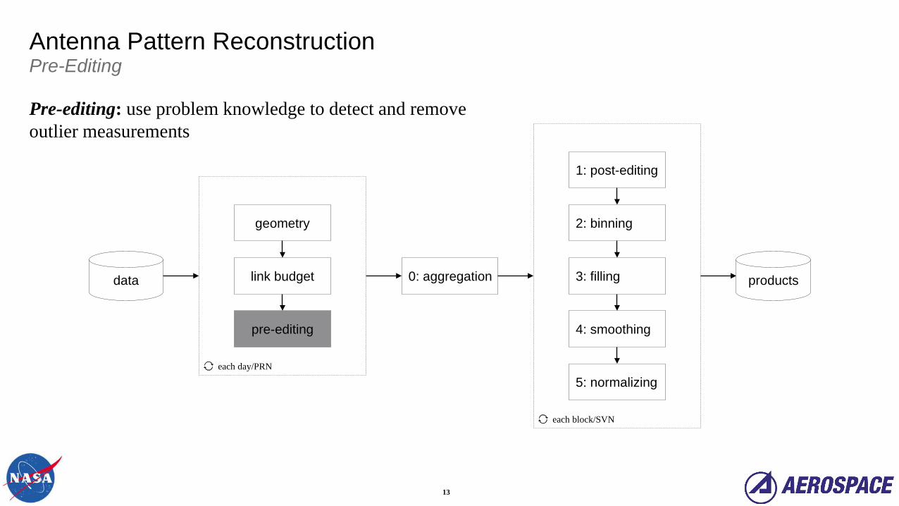
Antenna Pattern ReconstructionPre-Editing
geometry
link budget
pre-editing
each day/PRN
data 0: aggregation
1: post-editing
2: binning
3: filling
4: smoothing
5: normalizing
each block/SVN
products
Pre-editing: use problem knowledge to detect and remove outlier measurements

14
Data Editing: GPS SV AttitudeEclipse Periods
• Data was removed during noon and midnight turns• Yaw model accurately predicts when the turns will occur based on sun angle, spacecraft position, and
the beta angle.

15
Data Editing: GPS SV AttitudeYaw Excursions
• Automatic editing was implemented to catch anomalous tracking data.• In this case, the SV was commanded to an unexpected yaw attitude.

16
Antenna Pattern ReconstructionAggregation
geometry
link budget
pre-editing
each day/PRN
data 0: aggregation
1: post-editing
2: binning
3: filling
4: smoothing
5: normalizing
each block/SVN
products
0: Aggregation: collect PRN-specific data into SV-specific and block-average datasets

17
Antenna Pattern Reconstruction
geometry
link budget
pre-editing
each day/PRN
data 0: aggregation
1: post-editing
2: binning
3: filling
4: smoothing
5: normalizing
each block/SVN
products
1: Post-editing: perform outlier detection and removal at the pattern level2: Binning: Transform scattered measurements into a regular az/el grid
3: Filling: interpolate to fill isolated missing bins

18
Antenna Pattern ReconstructionSmoothing
geometry
link budget
pre-editing
each day/PRN
data 0: aggregation
1: post-editing
2: binning
3: filling
4: smoothing
5: normalizing
each block/SVN
products
4: Smoothing: Reduce noise in final pattern

19
Antenna Pattern ReconstructionSmoothing
• Smoothing– Binned and averaged data is noisy, used a low-pass filter to smooth

20
Antenna Pattern ReconstructionNormalization
geometry
link budget
pre-editing
each day/PRN
data 0: aggregation
1: post-editing
2: binning
3: filling
4: smoothing
5: normalizing
each block/SVN
products
5: Normalization: Calibrate the final patterns against known independent sources (e.g., ground-measured data)

21
Reconstructed vs. Ground: Azimuth Cut
• Reconstructed main lobe data is aligned to vendor ground measured data
• Shallow nulls– Some of these nulls are steep and
narrow (in azimuth). Yaw modeling errors contribute to averaging them out
– Possibly temporal effects (temperature, power variations, multipath)
• Most GPS receivers cannot track into the nulls so this information is not needed for accurate simulations

22
Reconstructed vs. Ground: Elevation Cut
• Good agreement in azimuth– Agrees well from main lobe out to the
second and third sidelobes (70 degrees off boresight)

23
Antenna Pattern ReconstructionProducts
geometry
link budget
pre-editing
each day/PRN
data 0: aggregation
1: post-editing
2: binning
3: filling
4: smoothing
5: normalizing
each block/SVN
products
24
In-Flight
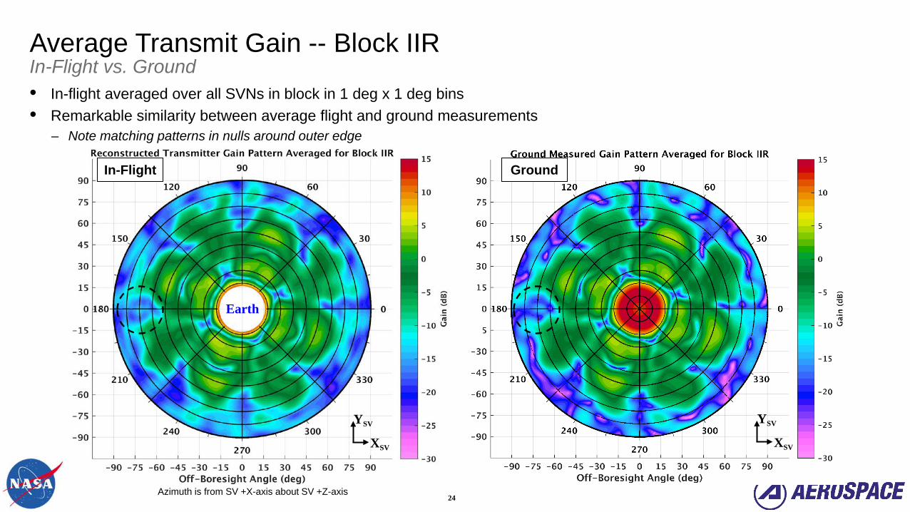
Average Transmit Gain -- Block IIRIn-Flight vs. Ground• In-flight averaged over all SVNs in block in 1 deg x 1 deg bins• Remarkable similarity between average flight and ground measurements
– Note matching patterns in nulls around outer edge
Earth
XSV
YSV
XSV
YSV
Azimuth is from SV +X-axis about SV +Z-axis
Ground
25
In-Flight
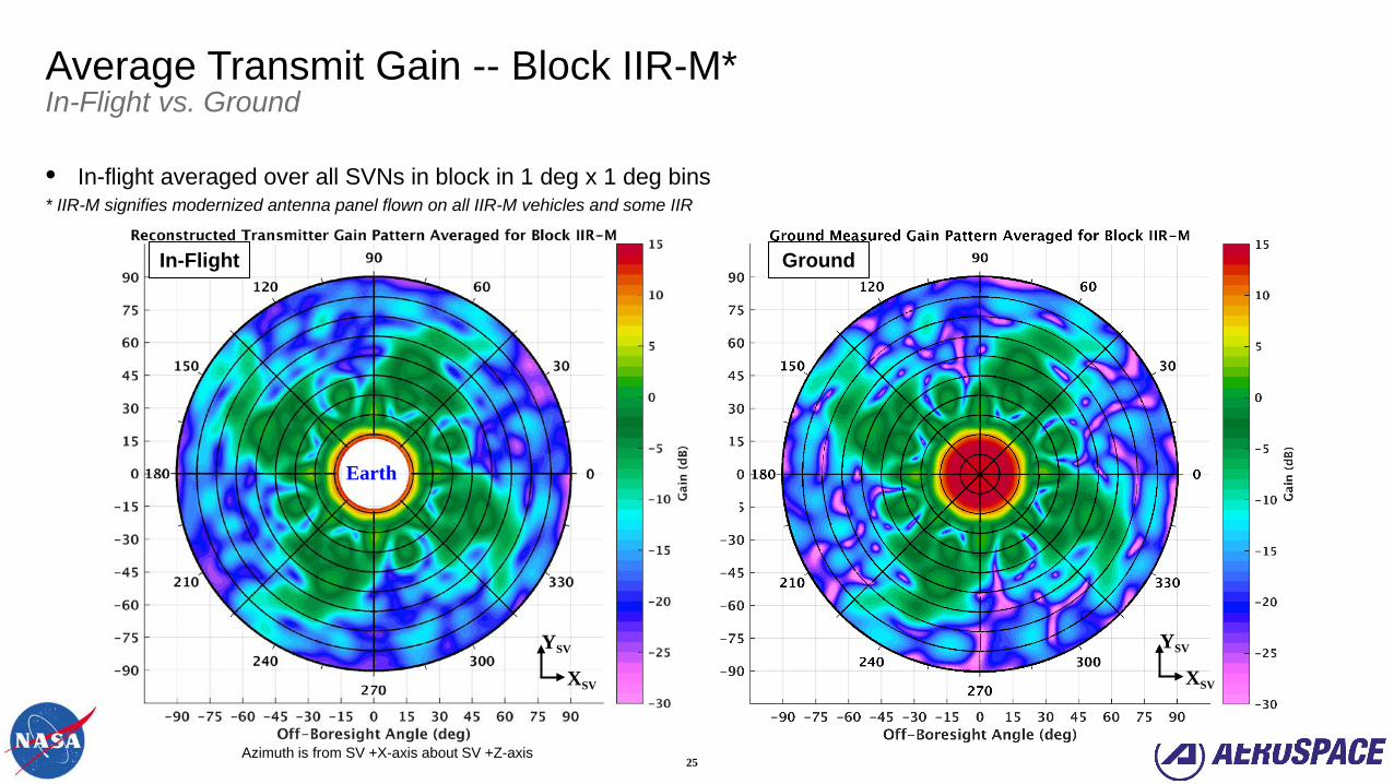
Average Transmit Gain -- Block IIR-M*In-Flight vs. Ground
• In-flight averaged over all SVNs in block in 1 deg x 1 deg bins* IIR-M signifies modernized antenna panel flown on all IIR-M vehicles and some IIR
Earth
XSV
YSV
XSV
YSV
Azimuth is from SV +X-axis about SV +Z-axis
Ground

26
IIA
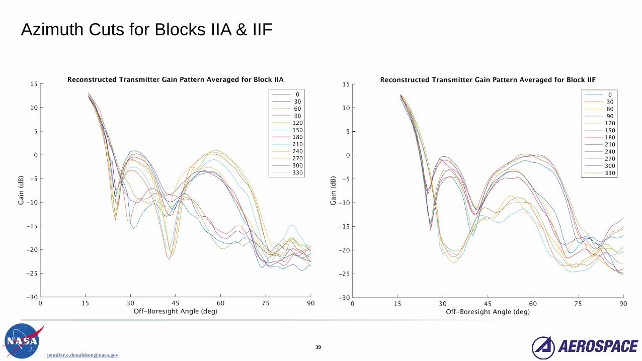
Average Transmit Gain -- Block IIA/IIFFirst Characterization of Full Transmit Patterns
• Averaged over all SVNs in block in 1 deg x 1 deg bins • IIF side lobes are shifted 45 deg in azimuth from other blocks
Earth
XSV
YSV
XSV
YSV
Azimuth is from SV +X-axis about SV +Z-axis
IIF
Earth

27
Gain vs. Off Boresight
Block Average vs. Individual SVNBlock IIF vs. SVN 70 Gain
• Close match between reconstructed block average patterns and individual patterns
Gain vs. Azimuth

28
Variation in Individual SVN GainMean Gain Difference
• There are mean differences in gain between patterns (before normalization)– Transmit power was applied uniformly to each block in the link budget
• These differences represent both the uncertainty in the link budget as well as differences in transmit power between individual satellites in a block

29
Pseudorange Deviation Analysis
• Evaluate pseudorange accuracy in side lobes• Create residuals from pass-through process:
– Use Aerospace TRACE high fidelity orbit determination tool
– Pass through external post-fit ephemeris– Compute residuals at all signal levels– Plot mean and standard deviation as a function of C/N0
for each block• Mean shows values < 1 m at all but extreme C/N0
– General negative trend at lower C/N0
– Spread in main beam likely due to atmosphere• St. Dev. shows remarkable agreement across
blocks– Noise function determined for relative weighting

Conclusions & Future Work
• GPS ACE architecture permits tracking of extremely weak signals over long duration– MGPSR produces signal measurements well into back lobes of GPS vehicles– 24/7 GPS telemetry provides near continuous tracking of each PRN
• First reconstruction of full GPS gain patterns from flight observations– Block averages of IIR, IIR-M show remarkable consistency with ground patterns
• Demonstrates value in extensive ground testing of antenna panel– Characterized full gain patterns from Blocks IIA, IIF for the first time– Patterns permit more accurate simulations of GPS signal availability for future HEO missions
• Pseudorange deviations indicate usable measurements far into side lobes• Future analyses include
– Signal level and measurement stability / variability over time– Comparison to GPS signals received by the highly elliptical NASA MMS Mission– Characterization of GPS Block III transmit antennas

Thank You
Dataset available at: https://esc.gsfc.nasa.gov/navigation


Antenna Pattern ReconstructionNASA GSFC OD Toolbox (ODTBX) Framework
• Geometry: capture problem geometry and calculate GPS transmit antenna-relative (az, el) for each measurement
• Link budget: reconstruct the transmit antenna gain value from a received C/N0measurement
• Pre-editing: use problem knowledge to detect and remove outlier measurements
• 0: Aggregation: collect PRN-specific data into SV-specific and block-average datasets
• 1: Post-editing: perform outlier detection and removal at th epattern level
• 2: Binning: Transform scattered measurements into a regular az/el grid
• 3: Filling: interpolate to fill isolated missing bins
• 4: Smoothing: Reduce noise in final pattern • 5: Normalization: Calibrate the final patterns
against known independent sources (e.g., ground-measured data)

34
Link Budget
• Link Budget– Knowledge of C/N0 and estimate of receiver noise temperature gives an estimate of the RX
power, Rp
– Estimate or calculate the RX antenna gain , Ar, the space loss, Ad, the GPS transmit power, Psv, and other losses, As and Lr, to find the TX antenna gain, At
𝐴𝐴𝑡𝑡 𝜃𝜃,𝜑𝜑 = �𝐶𝐶 𝑁𝑁0 − 𝑁𝑁0 − 𝐴𝐴𝑟𝑟 + 𝐿𝐿𝑟𝑟 + 𝐴𝐴𝑠𝑠 − 𝑃𝑃𝑠𝑠𝑠𝑠 − 𝐴𝐴𝑑𝑑

35
MGPSR Data CollectionHistograms of Single Day of Observations
• Plots show MGPSR data collection over 24 hours from GEO vehicle– Demonstrates spectrum of observations available daily for months
• Left plot shows sensitivity into back lobes (> 90 deg off-nadir / off-boresight)• Right plot shows received C/N0 sensitivity to < 0 dB-Hz
Block Total ObsIIA 4.8MIIR 19.1MIIR-M 26.3MIIF 21.1M

Antenna Pattern Reconstruction
• Link Budget– Knowledge of C/N0 and estimate of
receiver noise temperature gives an estimate of the RX power, Rp
– Estimate or calculate the RX antenna gain , Ar, the space loss, Ad, the GPS transmit power, Psv, and other losses, As and Lr, to find the TX antenna gain, At
• Smoothing– Binned and averaged data is noisy
using a moving window filter• Normalizing
– The patterns are matched to ground measured data 𝐴𝐴𝑡𝑡 𝜃𝜃,𝜑𝜑 = �𝐶𝐶 𝑁𝑁0 − 𝑁𝑁0 − 𝐴𝐴𝑟𝑟 + 𝐿𝐿𝑟𝑟 + 𝐴𝐴𝑠𝑠 − 𝑃𝑃𝑠𝑠𝑠𝑠 − 𝐴𝐴𝑑𝑑

GPS ACE Applications
• GPS ACE Data– Mission design/requirements verification
• Confidence in predicted signal availability and performance– Mission operations / satellite selection augmentation
• Improved operational navigation efficiency and accuracy• GPS ACE System/Concept
– SSV monitoring• Continuous monitoring of signal performance, including new launches
– GPS III antenna pattern verification• Comparison to requirements


40
Pseudorange Deviation vs. GPS Off-Boresight AngleBlock IIF Results• Azimuth cuts every 15 deg show variation, but reflect general trend to small negative bias in side lobes• Average at each elevation across all azimuths• Consistent behavior a different minimum signal levels
• Side lobe pseudoranges show small biases and predictable noise• Clearly useful for high altitude space missions