characterization of fracking soil, sediment, and
TRANSCRIPT

The Pennsylvania State University
The Graduate School
Department of Mechanical and Nuclear Engineering
CHARACTERIZATION OF FRACKING SOIL, SEDIMENT, AND WASTEWATER
SAMPLES USING
COMPARATIVE NEUTRON ACTIVATION ANALYSIS METHOD
A Thesis in
Nuclear Engineering
by
Maksat Kuatbek
© 2018 Maksat Kuatbek
Submitted in Partial Fulfillment
of the Requirements
for the Degree of
Master of Science
December 2018

ii
The thesis of Maksat Kuatbek was reviewed and approved* by the following:
Kenan Ünlü
Professor of Nuclear Engineering
Director of Radiation Science and Engineering Center
Thesis Co-Advisor
Amanda M Johnsen
Assistant Research Professor, Radiation Science and Engineering Center
Thesis Co-Advisor
Arthur Thompson Motta
Professor of Nuclear Engineering and Material Science and Engineering
Chair of the Nuclear Engineering Program
*Signatures are on file in the Graduate School

iii
ABSTRACT
The accurate multi-elemental analysis of soil, sediment, and wastewater samples is
extremely important for the regulatory monitoring of oil and gas (O&G) development. This kind
of analysis is typically conducted using several conventional methods, such as inductively coupled
plasma optical emission spectrometry (ICP-OES) or mass spectrometry (ICP-MS). The main
objective of this study was to apply the neutron activation analysis (NAA) method for qualitative
and quantitative analysis of hydraulic fracturing samples and to evaluate its accuracy and
applicability.
In this work, seventeen solid (soil and sediment) and five liquid (wastewater) samples
collected from the wellbores within Pennsylvania were characterized. The analysis was conducted
at the Radiation Science and Engineering Center (RSEC) using the comparative neutron analysis
method. The Montana II Soil and Buffalo River Sediment certified standard reference materials
obtained from the National Institute of Standards and Technology were used as the comparators.
As the result of this research, the concentration of short-, intermediate-, and long-lived isotopes of
Cl, Mn, Eu, K, Na, As, La, Ca, Ba, Rb, Pa (thorium activation product), Cr, Fe, Hg, Sr, Sc, Se, Zn,
and Cs elements in fracking samples were determined with an accuracy of ppm (mg/g or mg/l).
The experimentally measured values then were analyzed for standard deviation and verified
through a quality control check, with the exception of cesium and chromium; thus, their values
were declared as non-certified.
The trace element concentration values of three oil and gas wastewater samples, which
were obtained by the Comparative NAA (CNAA), were compared with the most probable value
(MPV) results determined via an inter-laboratory study. The MPVs were evaluated using the
nonparametric statistical method on the results collected from 15 laboratories from the United
States, Canada, and Germany that used different equipment and techniques for wastewater
characterization. The comparison results were demonstrated in the percentage difference

iv
magnitudes that vary from 0.1% to 56.6%. There are several possible reasons that might cause such
a relatively high error, as the hydride concentration remained after dehydration, the mass error of
liquid samples (due to evaporation), the use of multiple vials during dehydration (sample
movement), and the fragmentation of target elements (due to unfulfillment of pulverization and
homogenization of dried crystals before sampling).

v
TABLE OF CONTENTS
List of Figures .......................................................................................................................... vii
List of Tables ........................................................................................................................... ix
Acknowledgements .................................................................................................................. xii
Chapter 1 Introduction ............................................................................................................. 1
1.1 Motivation and Objectives ........................................................................................ 1 1.2 Thesis Structure .......................................................................................................... 2
Chapter 2 Hydraulic Fracturing ............................................................................................... 4
2.1 Description of The Fracking Process ......................................................................... 5
2.2 Environmental impacts and Potential Risks ............................................................... 8
Chapter 3 Neutron Activation Analysis ................................................................................... 10
3.1 Background and Specifications of NAA ................................................................... 10 3.2 Neutron Interactions with Matter ............................................................................... 11 3.3 NAA Methods ........................................................................................................... 13 3.3.1 Single Comparator NAA .................................................................................... 13
3.3.2 Instrumental NAA .............................................................................................. 14 3.3.3 Comparative NAA ............................................................................................. 16 3.4 Applicability of NAA ................................................................................................. 17
Chapter 4 Radiation Science and Engineering Center NAA Facility ...................................... 19
4.1 The Penn State Breazeale Nuclear Reactor (PSBR) .................................................. 19 4.2 RSEC Radionuclear Applications Laboratory ........................................................... 21 4.2.1 The Automatic Sample Handling System (ASHS) ............................................ 21
4.2.2 The Counting System ......................................................................................... 22 4.3 PSBR Irradiation Fixtures .......................................................................................... 25
4.4 Neutron Flux Characterization of the Dry Tube 1 for Core 58 Loading .................... 27
4.4.1 Preparation of the Samples and Documentations .............................................. 29
4.4.2 Irradiation and Counting of the Samples ........................................................... 30
4.4.3 Analysis of the Collected Data .......................................................................... 32
Chapter 5 Fracking Soil, Sediment and Wastewater Samples ................................................. 38
Chapter 6 The Experiment ....................................................................................................... 41
6.1 Activity Prediction ..................................................................................................... 41 6.2 The Sample Preparation ............................................................................................. 42
6.3 The Sample Irradiation and Counting ........................................................................ 49
Chapter 7 Experimental Results ............................................................................................... 54

vi
7.1 Data Analysis ............................................................................................................. 54 7.2 Quality Control .......................................................................................................... 60 7.3 Interlabratory Comparison of Results ........................................................................ 62
Chapter 8 Conclusion and Future Works ................................................................................. 68
References ................................................................................................................................ 73
Appendix A Physical Specifications ................................................................................ 76
Appendix B NIST Certificates ......................................................................................... 77 Appendix C Activity Prediction Results .......................................................................... 84
Appendix D Analysis Results .......................................................................................... 89

vii
LIST OF FIGURES
Figure 2.1. Comparison of Well Sites... ................................................................................... 4
Figure 2.1.1. Map of shale gas basins in the USA. .................................................................. 5
Figure 2.1.2. Volumetric percentage of additives in fracking fluids ....................................... 7
Figure 3.2.1. Schematic representation of radioactive capture reaction .................................. 12
Figure 4.1.1. A map of the PSBR Core 58 Loading ................................................................ 20
Figure 4.2.1.1. The rotary sample holder of the ASHS (capacity is over 90 samples) ............ 22
Figure 4.2.2.1. Component diagram of instrumentation layout to perform automated
radiation counting .................................................................................................................... 23
Figure 4.3.1 Shape and design of the dry tubes (DT) .............................................................. 26
Figure 4.3.2 The terminus located in the Radionuclear Applications Laboratory (RAL). ...... 27
Figure 4.4.1.1. The cadmium covered wire positions within Dry Tube 1 with respect to fuel
rod ............................................................................................................................................ 30
Figure 4.4.3.1. The AR (Activity Ratio) within the DT1 (Dry Tube 1) ................................... 34
Figure 4.4.3.2. Measured thermal neutron flux within DT1 (Dry Tube 1). ............................. 35
Figure 4.4.3.3. Measured resonance neutron flux within DT1 (Dry Tube 1). ......................... 36
Figure 4.4.3.4. The thermal and resonance neutron flux peak positions within the DT1 in
regard to a PSBR fuel rod ........................................................................................................ 37
Figure 5.1. A picture of all tested fracking soil, sediment, and wastewater samples in their
original plastic containers.. ...................................................................................................... 38
Figure 6.1.1. The graphical user interface (GUI) of the Activity Prediction Tool.. ................. 42
Figure 6.2.1. The Se sample with a concentration of 100 ppm (on the left) and a standard
PTTS capsule with the Se sample loading (on the right).. ....................................................... 45
Figure 6.2.2. A picture of fracking and SRM samples placed into Bucket #1. ........................ 48
Figure 6.2.3. A picture of fracking and SRM samples placed into Bucket #2. ........................ 48
Figure 6.2.4. The aluminum bucket dimensions and sample loading patterns.. ...................... 49

viii
Figure 6.3.1. The workplace that was set up near the shadow shield corner. It was used to
prepare irradiated samples for gamma ray counting ................................................................ 51
Figure 7.1.1. A gamma spectrum obtained from counting Solid 01 Sample after the
'medium' decay period ............................................................................................................. 57
Figure 7.1.2. A gamma spectrum obtained from counting Liquid 01 Sample after the
'medium' decay period ............................................................................................................. 58
Figure 7.3.1. A comparison of manganese concentrations in oil and gas wastewater samples
in a graphical manner ............................................................................................................... 66
Figure A-1. The HPGe detector dimensions provided by the manufacturer ............................ 76
Figure D-1. A graphical comparison of sodium concentrations in oil and gas wastewater
samples... .................................................................................................................................. 100
Figure D-2. A graphical comparison of potassium concentrations in oil and gas
wastewater samples... ............................................................................................................... 100
Figure D-3. A graphical comparison of calcium concentrations in oil and gas wastewater
samples... .................................................................................................................................. 101
Figure D-4. A graphical comparison of strontium concentrations in oil and gas
wastewater samples... ............................................................................................................... 101
Figure D-5. A graphical comparison of barium concentrations in oil and gas wastewater
samples... .................................................................................................................................. 102
Figure D-6. A graphical comparison of iron concentrations in oil and gas wastewater
samples... .................................................................................................................................. 102

ix
LIST OF TABLES
Table 2.1.1. Chemical content of a fracturing fluid and specific purposes for hydraulic
fracturing operations ................................................................................................................ 7
Table 4.2.2.1. The outline of the spectrum analysis sequence steps and their purposes. ......... 24
Table 5.1. List of the analyzed samples ................................................................................... 39
Table 6.2.1. Typical trace impurities in Heraeus Suprasil 310 quartz glass ............................ 43
Table 6.2.2. Comparison of selenium saturation activities within original and evaporated
samples. .................................................................................................................................... 46
Table 6.2.3. The identification numbers and weights of the test samples................................ 47
Table 7.1.1. The list of elements of interest and their radionuclides with gamma-decay
energies used in this study ....................................................................................................... 55
Table 7.1.2. Trace element concentrations of Solid 01 Sample ............................................... 56
Table 7.1.3. Trace element concentrations of the fracking samples (Part 1). The values are
given in weight percent (wt%) ................................................................................................. 59
Table 7.1.4. Trace element concentrations of the fracking samples (Part 2). The values are
given in weight percent (wt%) ................................................................................................. 60
Table 7.2.1. A summary of quality control analysis for Bucket#1 .......................................... 62
Table 7.2.2. A summary of quality control analysis for Bucket#2. ......................................... 62
Table 7.3.1. A summary of inter-laboratory study. All values are represented in mg/l ........... 65
Table 7.3.2. The concentration and standard deviation values of some trace elements
measured using the NAA method. ........................................................................................... 65
Table 7.3.3. The percent difference magnitudes between MPV and NAA measured values.
................................................................................................................................................. 67
Table C-1. Calculated activities and dose rates for the end of short irradiation of Bucket #1
content after a decay period of 48 hours .................................................................................. 84
Table C-2. Calculated activities and dose rates for the end of short irradiation of Bucket #2
content after a decay period of 48 hours .................................................................................. 86
Table C-3. Calculated activities and dose rates for the end of short irradiation of Bucket #1
and Bucket #2 content after a decay period of 192 hours ........................................................ 88

x
Table C-4. Calculated activities and dose rates for the end of short irradiation of Bucket #1
and Bucket #2 content after a decay period of 552 hours ........................................................ 89
Table D-1. Experimentally determined trace element concentrations of HR SaH sample
using NAA method .................................................................................................................. 89
Table D-2. Experimentally determined trace element concentrations of BO1 sample using
NAA method ............................................................................................................................ 90
Table D-3. Experimentally determined trace element concentrations of BO2 sample using
NAA method ............................................................................................................................ 90
Table D-4. Experimentally determined trace element concentrations of Sample 02 Solid
sample using NAA method ...................................................................................................... 91
Table D-5. Experimentally determined trace element concentrations of Sample 03 Solid
sample using NAA method. ..................................................................................................... 91
Table D-6. Experimentally determined trace element concentrations of Sample 04 Solid
sample using NAA method ...................................................................................................... 92
Table D-7. Experimentally determined trace element concentrations of AMD cycle 2
sample using NAA method ...................................................................................................... 92
Table D-8. Experimentally determined trace element concentrations of AMD test 5 sample
using NAA method .................................................................................................................. 93
Table D-9. Experimentally determined trace element concentrations of AMD test 6
sample using NAA method. ..................................................................................................... 93
Table D-10. Experimentally determined trace element concentrations of HR Evop. Test 01
sample using NAA method ...................................................................................................... 94
Table D-11. Experimentally determined trace element concentrations of HR Evop. Test
02 sample using NAA method ................................................................................................. 94
Table D-12. Experimentally determined trace element concentrations of Raw flowhart
solid sample using NAA method ............................................................................................. 95
Table D-13. Experimentally determined trace element concentrations of FS3 Effluent
sample using NAA method ...................................................................................................... 95
Table D-14. Experimentally determined trace element concentrations of Marsellus
Flowback sample using NAA method. .................................................................................... 96
Table D-15. Experimentally determined trace element concentrations of Franklin
discharge sample using NAA method ...................................................................................... 96
Table D-16. Experimentally determined trace element concentrations of Sample 01 liquid
sample using NAA method ...................................................................................................... 97

xi
Table D-17. Experimentally determined trace element concentrations of Sample 02 liquid
sample using NAA method ...................................................................................................... 97
Table D-18. Experimentally determined trace element concentrations of Sample 03 liquid
sample using NAA method ...................................................................................................... 98
Table D-19. Experimentally determined trace element concentrations of Sample 04 liquid
sample using NAA method ...................................................................................................... 98
Table D-20. Experimentally determined trace element concentrations of Sample 05 liquid
sample using NAA method ...................................................................................................... 99
Table D-21. Experimentally determined trace element concentrations of HR Evop. Test
03 sample using NAA method. ................................................................................................ 99

xii
ACKNOWLEDGEMENTS
The following people played an important role in helping me to achieve everything I have
achieved by this point. That is why in this acknowledgment I want to express my sincere
thankfulness for all their support.
First of all, I would like to thank my co-advisers Professor Kenan Ünlü and Dr. Amanda
Johnsen for their guidance throughout my studies, for their help in and out of academic frames and
most importantly for their motivational support. I acknowledge and appreciate their supervision
and assistance; thus, I can gladly say that for me it was a privilege to work with them. I also thank
my peers and friends from office: Alibek Kenges, Gokhan Corak, Bryan Eyers, Adam Rau, Andrew
Bascom, and Colleen Mulhollan for going through essential discussions together that enhanced my
understanding in all conceptual questions of my thesis. I am grateful to the personnel of the
Radiation Science and Engineering Center, especially Brian Bennett, for allowing me to use his
shop for many hours while producing quartz ampoules.
Moreover, I am thankful to Dr. Nathaniel R. Warner and his student Travis Tasker for
providing us with test samples and the opportunity to become part of the inter-laboratory study.
Finally, and most importantly I thank my family: my parents - Zharylkasyn and Roza for
upbringing me a way that I became a person who always strives for improvement, my sisters for
believing in me and supporting me from far distance with their warm, and all my friends for being
my comrades in all ideas and beliefs.
1
Chapter 1
Introduction
1.1 Motivation and Objectives
The accurate multi-elemental analysis of wastewater, soil, and sediment samples is
extremely important for the regulatory monitoring of oil and gas (O&G) development. The output
of this analysis ensures that the concentration of constituent elements within those samples is not
exceeding the regulatory limits. Moreover, in case of potential contamination events, the results
can be used as a fingerprinting application for identifying O&G wastewaters and their headsprings
[1]; thus, the analysis must be very precise and carry both qualitative and quantitative characters.
The chemical characterization of O&G samples is challenging due to the complex sample
(solid and fluid) matrix. It is typically conducted using numerous techniques, such as inductively
coupled plasma with optical emission spectrometry (ICP-OES), inductively coupled plasma with
mass spectrometry (ICP-MS), direct plasma spectrometry (DCP), triple quadrupole inductively
coupled plasma with mass spectrometry (ICP-MS/MS), X-ray fluorescence (XRF), and ion
chromatography (IC). [1]. However, all these methods have limitations due to the sample matrix
specifications or certain deficiencies in the techniques. For instance, ICP-OES or ICP-MS can be
hampered for detecting metals in high salinity O&G wastewaters because of the signal suppression
caused by easily ionized elements such as Na and K. This matrix effect can be solved by simple
sample dilution, which can cause another problem associated with a lack of sensitivity and
exceeding the detection limits for trace metals of interest [1].
The motivation of this study is to apply the neutron activation analysis (NAA) method for
multi-elemental characterization of solid and liquid samples from fracking process. The

2
applicability of the NAA for this study will be evaluated by comparing its results with the results
of other methods. Moreover, this comparison allows the determination of the advantages and
disadvantages of the NAA, among other techniques, and to identify the elements for which the
NAA can provide reliable quantitative results. If NAA performs better on some or most of the
elements, it has the full potential to become a secondary or even primary application for O&G
regulation studies.
1.2 Thesis Structure
This thesis consists of eight chapters. This chapter will cover a brief description of the main
objectives and content of each part.
Chapter two discusses a quick overview of the history and future of hydraulic fracturing.
Moreover, the chapter provides a basic knowledge of the fracking process and its methodology.
The types and specifics of fracking fluids, their environmental impacts, and potential risks also
covered in this chapter.
Chapter three provides the background information about the neutron activation analysis
(NAA) technique and the theory behind it. The chapter also introduces the types of neutron
interactions with matter and the most common three NAA methods, such as the absolute NAA
method, comparative method, and single comparator NAA (known as k-factor method). At the end
of this chapter, the applicability of NAA is discussed through existing NAA applications in a wide
range of disciplines.
The fourth chapter describes the Radiation Science and Engineering Center (RSEC)
facilities employed in this research. In addition, this chapter provides a more detailed description
of the automatic sample handling system (ASHS), radiation counting system, the pneumatic tube
transport system (PTTS), and dry irradiation tubes. The detailed data on the neutron flux
characterization of the Dry Tube 1 for Core 58 loading are also given in this chapter.

3
A list of analyzed fracking solid (soil and sediment) and liquid (wastewater) samples are
presented in Chapter five. The chapter also provides brief descriptions and specifications of test
samples.
The experimental procedures for this study were divided into three stages and are described
in detail in Chapter 6. The first stage is activity prediction, which was performed using the Activity
Predictor program developed by Dr. Dağistan Şahin. At this step a rough design of the experiment
was determined regarding the choice of the suitable irradiation time and fixture (due to neutron flux
requirements), test sample mass and geometry, time of decay and radiation counting. The second
stage is sample preparation, which mainly describes the test sample weighing and encapsulating
activities. The last stage is the sample irradiation and counting that contains detailed information
on the conditions of irradiation and measurement.
Chapter seven presents the experimental results obtained through comprehensive data
acquisition and analysis. Furthermore, this chapter numerically demonstrates the quality control of
results and their comparison with the results of other laboratories and methodologies.
Chapter eight provides conclusions and a brief summary of this research. Further studies
and work suggestions are also commented on this chapter.

4
Chapter 2
Hydraulic Fracturing
Historically, gas-well drilling was performed using a single vertical well, which provided
access to conventional sources of gas that flowed through pore spaces along the wellbore (Figure
2.1). However, there are also unconventional gas reservoirs with low permeability formations that
require a different extraction technique. [2]. For this reason, a new method called “Hydraulic
fracturing”, commonly known as “fracking” was developed. This method allows extraction of
natural gas from deep shale strata by using a high-pressure drilling technique. The drilling process
combines the traditional vertical and additional horizontal drillings that allows injection of highly
pressurized fracking fluid into shale formation to keep fractures propped open, so gas can be
released and freely flow at a higher rate to the wellbore (Figure 2.1) [3] [4].
Figure 2.1. Comparison of Well Sites [5].
Even though the hydrofracking was first used in the 1940s, in practice, it was widely
applied only after the 1990s, when natural gas prices increased making fracking more financially
attractive [2]. Moreover, the latest advances and improvements in horizontal drilling, such as
multiple wells drilled from one surface location, have made this method even more productive and

5
economically competitive. Thus, in the last two decades, the number of natural gas wells in the
United States has increased by 200,000, which will allow gas production rate up to 1065 billion
cubic meters per year by 2040 [6]. This scale of production makes hydraulic fracturing a promising
new energy extraction technology of the 21st century [4].
2.1 Description of The Fracking Process
After detailed geological research of deep underground rock formations, the fracking
process starts with drilling and installing wells. A typical installation contains one to several wells
that are drilled from a single wellpad [7]. The fracturing depth depends on target shale stratum, so
major U.S. wells descend vertically from 150 m to more than 4000 m [8]. Figure 2.1.1 shows a
map of shale gas basins in the United States, which are separated and differently colored depending
on their depth and age. The map was prepared by Cidney Christie (Duke University), based on data
from U.S. Energy Information Administration (EIA).
Figure 2.1.1. Map of shale gas basins in the USA [9].

6
The horizontal leg of a gas well might continue as much as 1.5 km with discrete length
fractures of 91-152 m (Figure 2.1). In other words, a single horizontal well can allow up to 15
separate hydrofrack “events” simultaneously [2]. The rest of the hydraulic fracturing process can
be explained by three major steps: 1) fracture the rock formation by injection of fracking fluid
(water, sand, and chemical additives) to horizontal drilled well using high pressure; 2) extract and
collect the natural gas released from the shale through the well; 3) treat or dispose of the water that
was used for well fracking. Thus, one of the biggest challenges is the significant volumes of
ascended water that occurs after pressure release. The performance of hydraulic fracturing per well
requires about 2-5 million gallons of water [4]. Around 10 to 80 percent of the injected water may
return to the surface as wastewater. In the entire fracking process, there are two terms regarding
wastewater: flowback (fluid that quickly returns to the surface) and produced water (fluid that takes
longer to return to the surface). Since the injected fluid allows for the liberation of gas and materials
trapped in the shale, flowback and productive water are enriched with brines, hydrocarbons,
naturally occurring radioactive materials, and trace elements. In fact, the longer the fluid remains
in the shale the greater the concentration of native geological formation materials in it [10].
The content on the fracturing fluid varies, depending on the specific needs of the extracting
company and the geological characteristics of the fracking location. Moreover, the inventory and
exact concentration of chemical additives in fracking waters remains confidential; however, it is
possible to roughly evaluate the percentage of volumes of fracking fluid by using general
knowledge about fracking basics and widely reported documents. Overall, the concentration of
different chemical additives in vast fracking fluids is relatively small and vary between 0.5-2%, so
the remaining 98-99.5% of fluid contain water and proppants (silica sand) [5]. The typical
volumetric percentage of additives that were used for a regular fracking treatment is demonstrated
in figure 2.1.2.

7
Figure 2.1.2. Volumetric Percentage of Additives in Fracking Fluids [4].
Table 2.1.1 shows the list of major additives, their chemical composition, volumetric
percentage, and a brief explanation regarding a specific purpose of usage.
Table 2.1.1 Chemical content of a fracturing fluid and specific purposes for hydraulic
fracturing operations [4].
However, wastewater (especially produced water) may contain an even wider range of
isotopes than was originally added to the injected water. This phenomenon occurs due to the
mixture of injected water with naturally occurring water in the geologic shale. Thus, the natural
components of the formation will be present in the wastewater when it is recovered from a well
after a long-term period. These substances can originate from the water, rock, oil or gas present in
the formation [4]. Below are described a couple of the most significant classes of constituents:

8
• Naturally occurring radioactive materials, such as uranium, thorium, radium, radon,
strontium and potassium [4]. Some research results demonstrate that flowback and produced
water samples contain relatively high concentration of radioactive material. For example, in
a produced water sample from the Marcellus Shale showed radium and uranium
concentrations at the pCi/L level [11]. Similarly, another study identified radium in produced
waters from the Northern Appalachian Basin [4].
• Inorganic substances and metals, such as aluminum, arsenic, barium, bromine, cadmium,
chloride, chromium, iron, manganese, mercury, nickel, sodium, vanadium and zinc. By
nature, the salinity of formation water is very high, so Cl, Na, and Br are the most common
detected elements. Moreover, there are also a list of regularly detected elements from
produced water samples. For example, Ba, Br Ca, Cl, Na, and Sr were common for the
Marcellus Shale basin waters [4].
2.2 Environmental Impacts and Potential Risks
Even though the volumetric percentage of additives in the injected water is very small, the
total amount of chemicals is still significant due to the volume of used water (up to 5 million gallons
per well). Regardless of the level of dilution, this amount of chemicals might carry a potential risk
to the local environment and public health. This fact raised public concerns about fracking, so
scientists started to collect data, analyze, and evaluate the potential risks based on local
environmental impacts. The major potential risks are related to water contamination, air pollution
(large and high-density gas emission), seismicity (small earthquakes), and local landscape changes
[3].
The biggest concern was regarding the potential contamination of water resources, which
includes: 1) stray gas contamination of shallow groundwater that located above shale gas basins;
2) the contamination of pathways and hydraulic connections between shallow drinking water
9
aquifers and the deep shale gas formations; 3) inadequate treatment or disposal of wastewater
(flowback and produced water) that causes surface water contamination and long-term ecological
effect [9]. In the case with wastewater disposal everything is relatively straight forward, since this
problem can be regulated by developing new policies. For example, on May 19, 2011 the
Pennsylvania Department of Environmental Protection (PADEP) prohibited to drilling companies
to dispose their wastewater through wastewater treatment plants (WWTPs) [10]. Nevertheless, it is
more challenging to predict and prevent the shallow water aquifer pollution, since contaminants
can potentially be transported through both bulk media (advective way) and fractures (preferential
flow). Moreover, there is a significant proof that the natural vertical flow also drives contaminants
(mostly brine) close to the surface from deep evaporate sources [12]. Thus, it is even more
challenging to sensitively distinguish the contaminations caused by hydraulic fracturing activities
from the pollution due to the natural flow. Recent studies conducted in Marcellus Formation have
shown that strontium isotope ratios (87Sr/86Sr) can be used to investigate the origin of total dissolved
solids (TDS) in ground and surface water [13].

10
Chapter 3
Neutron Activation Analysis
Neutron Activation Analysis (NAA) is a very sensitive, non-destructive analytical method
for determining the major, minor, and trace elements of a sample material. Moreover, this technique
allows both qualitative and quantitative multielement analysis. Within proper conditions, NAA is
capable to quantitively identify up to 60 elements in small samples, usually with masses of
milligram. The lower detection limit of NAA varies due to the element or isotope of interest and
typically ranges on the order of parts per million (ppm) to parts per billion (ppb).
3.1 Background and Specifications of NAA
Neutron Activation Analysis was discovered in 1936 by George de Hevesy and Hilde Levi,
when they were performing a quantitative analysis on rare-earth salts by exposing them with
neutrons naturally emitted from Ra(Be) source [14]. In the 1950s and 1960s, the potential of NAA
as an experimental method drastically increased due to more detailed research on the notions such
as, decay, characteristics of radiation absorption, and radiochemical separation. Also, the
introduction of scintillator and semiconductor detectors provided selectivity in gamma-ray
spectrometry, so the individual radionuclides can be identified mostly without initial chemical
separations [15]. The principal involved in NAA consists of bombarding the specimen with
neutrons in a suitable irradiation facility (typically a nuclear research reactor) to produce specific
radionuclides. Following irradiation, the artificially created radionuclides undergo decay to reach
their ground state configurations by emitting beta particles and characteristic gamma rays. Because
each radioactive isotope always emits characteristic gamma rays at unique energies and intensities,

11
the quantitative measurement of those gamma rays by gamma spectroscopy provides information
on the radioisotopes present, and hence the parent chemical element(s).
3.2 Neutron Interactions with Matter
Neutrons are electrically neutral, so when they interact with matter, they cannot be affected
by the Coulomb force of either the atomic electron cloud of an atom or the positively charged
nucleus. Therefore, neutrons do not interact with the atom, but directly with the nucleus. The
probability that a neutron interacts with a nucleus is quantitatively described by the term known as
cross-section. The interaction of a neutron with a nucleus may follow one or more of these
reactions: elastic scattering, inelastic scattering, radiative capture, charged-particle reactions,
neutron-producing reactions, and fission [16]. Each reaction has its own cross-sectional value, and
their sum is equal to the total cross-section. Some of these reactions are defined below.
Elastic scattering is when a neutron collides with a nucleus of an atom without changing
its intrinsic composition (number of neutrons and protons) and energy level. All of the kinetic
energy of the incoming neutron is divided between two particles, so after the collision, they recoil
from each other with different speeds and directions. Thus, in the elastic scattering, the nucleus
remains in the initial ground state, despite the energy transfer. In the notation of nuclear reactions,
this reaction is commonly abbreviated as (n,n), demonstrating that the neutron interaction has not
caused any fundamental changes to the nucleus.
Inelastic scattering is a similar process to elastic scattering, except that some portion of the
kinetic energy retained by the nucleus converts to internal energy (an endothermic interaction), so
the nucleus moves from the ground state to the excited state. The excited nucleus eventually decays,
emitting gamma ray(s) (inelastic 𝛾-ray(s)) and returning to its initial ground state. Inelastic
scattering is typically denoted by (n,n’) symbol.

12
Radiative capture or neutron absorption is a reaction when the nucleus captures the
colliding neutron and changes its mass and energy. The probability of this event is described by the
neutron capture cross-section, which varies with respect to the size and stability of the target
nucleus, and the energy of incident neutron. After the capture, the excess energy will be
immediately (usually within 10-14 seconds) emitted in the form of prompt gamma ray. The newly
formed nucleus is often still unstable (radioactive), so it will beta decay to a stable state by emitting
a beta particle and one or more subsequent (delayed) gamma rays with fixed half-life times (Figure
3.2.1). The time frame for the emission of delayed gamma rays ranges from seconds to days, or
even up to months.
Figure 3.2.1. Schematic representation of radioactive capture reaction [17].
Measuring the prompt gamma rays is often experimentally complex for the neutron
activation analysis. However, the delayed gamma rays can be measured relatively easily by HPGe
detectors and later analyzed for individual radionuclide identification. The delayed gamma rays are
extremely important for NAA, as they carry specific decay energy information about the element

13
in the material that can be used as a fingerprint to identify this element, including its multiple
isotopes [16]. Radiative capture is denoted by the notation (n,γ).
3.3 NAA Methods
NAA is a powerful, precise, and versatile analytical technique suitable for the analysis of
many types of samples, hence it is actively employed in a wide range of disciplines such as
archaeology, geochemistry, health and human nutrition, semiconductor technology, and
environmental monitoring [18]. Depending on applications, tested samples, experiment conditions
and objectives, NAA can be customized and performed with a different methodology. All NAA
methods use the same principle that was discussed in Section 3.1; however, they differ from one
another in sample irradiation and data analysis. Each method has advantages and disadvantages.
The most common three NAA methods will be briefly discussed in the following sections.
3.3.1 The Absolute NAA Method
The absolute NAA method, also known as instrumental neutron activation analysis
(INAA), determines the absolute elemental or isotopic concentration in the test sample material,
directly using the measured experimental parameters, such as the activity of the irradiated sample
and local neutron flux (Equation 3.3.1.1).
A = N(1 – e-λt)[ σthΦth + σresΦres] (3.3.1.1)
In equation 3.1, A (measured activity), N (number of atoms), λ (decay constant) values are
associated with an irradiated element in the sample, t is the decay time between the end of
irradiation and the beginning of radiation counting, σth (thermal) and σres (resonance) are the neutron
absorption cross-sections, and Φth (thermal) and Φres (resonance) are neutron flux magnitudes
measured at the sample irradiation location [19].

14
This method is very sensitive to the accuracy of measured values, so it is extremely
important to use proper procedure and equipment to obtain adequate results. Thus, for the sample
activity measurement high resolution HPGe detectors are typically used. Nevertheless, the
efficiency and calibration of these detectors might slightly vary, due to the small parameter changes
regarding sample geometry, orientation, etc. One of the disadvantages of INAA is the fact that it is
challenging to avoid small changes during the radiation counting and irradiation, which might
significantly affect the final results. Another challenge within this method is related to measuring
accurate local neutron flux values and determining the exact number of activated atoms due to the
neutron flux exposure. For high precision, it is also important to take into account the self-shielding
of the sample. In practice, it is difficult to maintain identical efficiency and calibration of the
detector and to measure the neutron flux value for each sample location; therefore, this method is
more applicable when there are only a few samples with the same size and relatively simple
elemental composition [20].
The absolute NAA method was not found suitable for this work, since the objective of this
work was a characterization of 22 fracking soil and water samples that have very complex elemental
compositions.
3.3.2 Comparative NAA
Comparative NAA (CNAA), also called the relative calibration method, is another
approach that avoids some of the drawbacks of the absolute NAA method while determining the
concentration of an element/isotope in a sample. In order to perform CNAA, it is necessary to have
rough knowledge regarding the elemental/isotopic content of the test sample and one or more
standard materials of similar content. The sample(s) and standard(s) must be irradiated and counted
under the same conditions. The elemental/isotopic concentrations in the unknown (tested) sample
are determined using Equation 3.3.2.1.

15
𝑤𝑢 = 𝑚𝑠𝐴𝑢𝐷𝑢𝐶𝑢Φ𝑠
𝑚𝑢𝐴𝑠𝐷𝑠𝐶𝑠Φ𝑢 (3.3.2.1)
Where the subscripts u and s refer to the unknown and standard used in the comparison, 𝑤
is the concentration of the element of interest, m is the mass of the sample, A is the measured
activity of the target isotope (including the detector efficiency, the saturation factor, etc.), D is the
decay correction factor, C is the counting correction factor, and Φ is the exposed neutron flux. The
decay correction factor for each sample can be calculated via Equation 3.3.2.2.
𝐷 = exp (−λ𝑡𝑑) (3.3.2.2)
Where λ is the decay constant of the isotope of interest, and 𝑡𝑑 represents the time between
the end of irradiation and beginning of radioactive counting. The counting correction factor is more
important during long radioactive counting, since it is accounting for decay during the measurement
(Equation 3.3.2.3).
𝐶 = 1−exp (λ𝑡𝑚)
λ𝑡𝑚 (3.3.2.3)
The variable 𝑡𝑚is the radioactive counting time.
CNAA has a clear advantage over other NAA methods, if the suitable comparator standard
and the test sample have a similar geometry, background matrix, and trace element composition
[19] [20]. By irradiating test and standard samples together, it is possible to eliminate the necessity
for an accurate knowledge of the neutron flux, assuming that both samples exposed an equivalent
neutron flux. Moreover, using CNAA method, there is no need to evaluate the detector efficiency,
calibration, and counting geometry effects as it was required by INAA. Therefore, the
ascertainment of the composition of trace elements is performed more simply with CNAA
compared to INAA. The main disadvantage of CNAA is that it becomes inapplicable and useless
with the absence of a suitable standard material for the desired sample matrix, which includes the
elements of interest [19].

16
3.3.3 Single Comparator NAA
Single Comparator NAA, also known as k-factor method, is another comparative approach
to perform multi-element analysis of an examined sample. This method was first critically
evaluated by F. De Corte [21] and later was found very useful in the cases where the implementation
of CNAA method is impossible due to the unavailability or exorbitant cost of suitable standard
materials. As the term single comparator refers, this method differs from traditional CNAA by
irradiating, measuring, and comparing only a single element material (mostly gold) as a standard.
In practice, a typical comparator material is a small piece of gold foil or wire. Due to the small size
of the comparator, it can be placed next to the sample during irradiation, thereby ensuring the
equivalent effect of the neutron flux expose (Φ/ Φ*=1) [21].
The determination of the elemental concentration of test sample is based on the ratio of
proportionality factors of the target and comparator elements that defined as k-factor value. The
experimentally-determined k factor can be calculated using the following equations [21]:
𝑘 =𝐴𝑠𝑝
𝐴𝑠𝑝∗ =
𝑀∗
𝑀∙
𝛾
𝛾∗ ∙𝜖𝑝
𝜖𝑝∗ ∙
𝛩
𝛩∗ ∙Φ
Φ∗ ∙𝜎
𝜎∗ (3.3.1.1)
with 𝐴𝑠𝑝 =𝐴𝑝
𝑆∙𝐷∙𝐶∙𝑤 (3.3.1.2)
where <*> sign refers to the single comparator or monitor, and absence of any sign indicated the
unknown sample. The variable Asp is the specific count rate, M is the atomic weight of the irradiated
element, Θ is the isotopic abundance of the target nuclide, γ is the absolute abundance of the
measured γ-ray, ϵp is the full-energy peak efficiency of the detector for the measured γ-ray energy,
Φ is the conventional reactor neutron flux [neutron/(cm2∙sec)], σ is the effective reactor neutron
cross-section [b], Ap is the measured average intensity of the full-energy peak [counts/sec], w is the
weight of the element [g], D is the decay factor, and C is a measurement correction factor. The
activity saturation factor (S) dependent on the decay constant (λ), and the irradiation time, (tirr). The
dependency shown in Equation 3.3.1.3.

17
𝑆 = 1 − exp (−λ ∙ tirr) (3.3.1.3)
Calculations using these experimentally determined k-factors are usually more accurate
than calculations of the absolute calibration method, based on literature data [21]. Nevertheless, the
k-factors are very dependent on the measured experimental conditions, so small variations in
neutron flux rate, detector efficiency, or counting geometry can cause a significant error and make
the method invalid [19]. The k-factor determination requires very precise and laborious
experimental work, once they are available there is no need for preparation of standards for further
analysis. The determined k-factors are assumed to be constant as long as there are no variations in
the quantities given in Equation 3.3.1.1 [21].
Comparing these three NAA methods, it was decided to use the comparative method
(CNAA) in this work for several reasons. First, two suitable soil and sediment standard materials
were available for comparison to the fracking samples. Second, the samples were in forms of
powder (soil and sediment) and crystal (dried water), which makes them easy to encapsulate and
shape to similar geometries. Next, CNAA method is more accurate due to less sensitivity to the
changes in the measurement parameters. Finally, data analysis using the CNAA method was found
relatively more straightforward than other methods.
3.4 Applicability of NAA
Like any other method for determining trace elements, the neutron activation analysis is
not completely universal and applicable to all types of materials. The chemical properties, physical
forms, and physical characteristics of the sample are important accounting factors for applicability
of NAA to a specific work. Another essential factor is the element of interest and nuclear properties
of its isotopes, since it influences to the activation rate (absorption cross-section) and decay
characteristics of produced radionuclide (half-life, gamma ray abundance and energies). Therefore,
the very low Z elements (like H, He, B, Be, C, N, and O) and a few other elements (Tl and Bi) are

18
not suitable for NAA characterizations. Some elements such as lead (Pb) can be determined with
low sensitivity (order of milligrams) and useless for many applications. The sample matrixes with
both high density (high atomic number) and very high neutron absorbing properties are also
unwanted, due to strong gamma-ray self-attenuation. High concentrations of the elements (B, Li,
and U) that emit charged particles (α-radiation) after neutron absorption are also not preferable,
since they cause active thermal heating during the continuous irradiation [15].
Despite all these specifics, neutron activation analysis is widely implemented in numerous
disciplines, such as archaeology (metal, stone, pottery artifacts, etc.), biomedicine (tissue, blood,
venom, etc.), environmental science and related fields (aerosols, fossil fuels and fuel, sediments,
etc.), forensics (bomb debris, bullet lead, shotgun pellet, etc.), geology geochemistry (coal and oil
shale components, cosmo-chemical samples, diamonds, etc.), industrial products (alloys, electronic
material, high purity and high-tech materials, semiconductors, etc.), and nutrition (composite diets,
spices, milk and milk formulae, etc.) [15].
In this work, neutron activation analysis technique is used to characterize the soil and water
samples collected from hydraulic fracturing wellbores. The accurate multi-element analyses of
wastewater and soil samples are extremely important for the regulatory monitoring of oil and gas
(O&G) development. The NAA might be an excellent tool for this analysis because it provides very
accurate qualitative and quantitative results in terms of concentrations of constituent elements,
which are used to ensure that everything is within regulatory limits.
19
Chapter 4
Radiation Science and Engineering Center NAA Facility
The experimental part of this work was conducted on the base of Radiation Science and
Engineering Center (RSEC), which houses multiple nuclear research and education facilities, such
as the Penn State Breazeale Reactor (PSBR), Co-60 Gamma Ray Irradiation Facility, Hot Cells,
Radiochemistry Teaching and Research Laboratory, Subcritical Graphite Reactor Facility, the
neutron beam laboratory, Radionuclear Applications Laboratory (RAL), and Nuclear Security
Education Laboratory[22]. The main missions of the RSEC are education (faculty, staff, students,
and public), training (NRC certified reactor operators, inters), and research (NAA, reactor control,
and various neutron beam techniques, etc.). Moreover, using the Penn State Breazeale Reactor
(PSBR) and other irradiation facilities, the RSEC is also provided irradiation services to other
universities, government entities, and the industry [23].
4.1 The Penn State Breazeale Nuclear Reactor (PSBR)
The Penn State Breazeale Nuclear Reactor (PSBR) is the first licensed and longest
continuously operating university research nuclear reactor in the United States, which reached its
first criticality in 1955. The reactor originally was designed as a material test reactor (MTR) that
uses a plate type fuel made of highly enriched uranium. However, after receiving a license
amendment in 1965, the reactor was converted to a TRIGA (Training, Research, Isotopes, General
Atomics) design that operates on a low-enriched uranium-based pin type fuel [22]. The current
TRIGA MARK III reactor core resides on the bottom of 24 feet deep open-pool that is filled with
approximately 71,000 gallons of deionized water. The core is attached to a bridge on rails, so it can
be moved in several directions throughout the pool, providing the flux flexibility for the out-core
irradiation fixtures. In steady state operation, the maximum power of PSBR is rated as 1 MW and

20
the maximum thermal neutron flux in the central thimble is about 3*1013 n/cm2s. The PSBR also
has a pulsing ability at which the reactor power can reach 2000 MW for 10 milliseconds and the
thermal neutron flux peak reaches up to 1016 n/cm2s [19].
In this work, the PSBR core loading number 58 was used for the flux profile determination
(section 4.4) and fracking sample irradiation (section 6.3). The map of the core loading number 58
is shown in Figure 4.1.1.
Figure 4.1.1. A map of the PSBR Core 58 Loading
Figure 4.1.1 shown the pattern of the TRIGA pin fuels that contain 8.5 wt% and 12 wt%
low enriched uranium. Moreover, there are demonstrated the locations of the control rods (F9, H6,
H12, and J9), dry tubes (E6 and E11), and central thimble (H9). The multiplicity of irradiation

21
locations and the flexibility of neutron flux makes PSBR a perfect source for NAA applications
[19].
4.2 RSEC Radionuclear Applications Laboratory
The RSEC also houses radionuclear applications laboratory (RAL) that provides technical
support to radionuclear technique users, such as research personnel and industrial users. The
laboratory has a convenient workstation with all necessary equipment for sample preparation and
post-irradiation handling, four complete high-purity germanium detector (HPGe) systems, two
automatic sample handling systems (ASHS), a pneumatic tube transport (rabbit) system terminus,
a Compton Suppression System and multiple Geiger-Mueller (GM) “Pancake” detectors and
Genie-2000 software installed computers [22] [19]. In the following sections will be discussed the
ASHS and HPGe detector system, which were used for radiation counting in this study.
4.2.1 The Automatic Sample Handling System (ASHS)
The automatic sample handling system (ASHS) is an essential tool for all NAA sample
measurement since it operates in conjunction with a radiation counting system and automates the
process. The automation of radiation counting provides additional reliability and consistency of
measurements because it minimizes the error due to counting statistics by reducing the decay time
between sample measurements.

22
Figure 4.2.1.1. The rotary sample holder of the ASHS (capacity is over 90 samples).
The ASHS has a rotary sample tray that is capable to hold over 90 samples (Figure 4.2.1.1).
The sample tray moves each sample one at a time under a pneumatic lever, which picks up and
places the sample into a nest 2.5 cm above of the HPGe detector. When the counting is completed,
the ASHS automatically picks up the remaining sample and replaces it with a next sample. The
user can select counting parameters, such as counting time (from seconds to days) and the number
of samples to be counted (from 1 to 90).
4.2.2 The Counting System
Once the ASHS moves the sample into sample nest, it is measured with a counting system
that includes a Canberra GC1518 HPGe detector, a digital spectrum analyzer (DSA-2000), and a

23
personal computer (PC) with Canberra’s Genie-2000 software. All these radiation detection and
measurement instrumentations and ASHS are connected as it is demonstrated in Figure 4.2.2.1.
Figure 4.2.2.1. Component diagram of instrumentation layout to perform automated
radiation counting [22].
To reduce the background radiation, the HPGe detector is placed into lead shielding cave
with an internal copper and tin liner. These liners contribute to eliminating X-rays caused by the
interaction of gamma rays with lead. The manufacturer specifications and dimensions of the HPGe
detector shown in Appendix A.
The DSA-2000 is a fully integrated system for high quality spectrum acquisition. It
combines the digital signal processor (DSP), high voltage (HV) power supply, digital stabilizer,
multi-channel analyzer (MCA) memory, and an Ethernet network interface. The DSA-2000 and
the PC are connected via cable, and they communicate through Genie-2000 software, which
visualizes the count information for each channel in the real time.
24
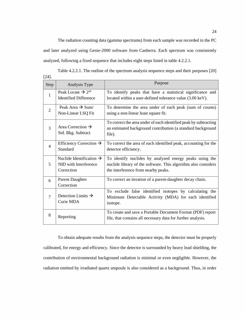
The radiation counting data (gamma spectrums) from each sample was recorded in the PC
and later analyzed using Genie-2000 software from Canberra. Each spectrum was consistently
analyzed, following a fixed sequence that includes eight steps listed in table 4.2.2.1.
Table 4.2.2.1. The outline of the spectrum analysis sequence steps and their purposes [20]
[24].
Step Analysis Type Purpose
1 Peak Locate → 2nd
Identified Difference
To identify peaks that have a statistical significance and
located within a user-defined tolerance value (3.00 keV).
2 Peak Area → Sum/
Non-Linear LSQ Fit
To determine the area under of each peak (sum of counts)
using a non-linear least square fit.
3 Area Correction →
Std. Bkg. Subtract
To correct the area under of each identified peak by subtracting
an estimated background contribution (a standard background
file).
4 Efficiency Correction →
Standard
To correct the area of each identified peak, accounting for the
detector efficiency.
5
Nuclide Identification →
NID with Interference
Correction
To identify nuclides by analyzed energy peaks using the
nuclide library of the software. This algorithm also considers
the interference from nearby peaks.
6 Parent Daughter
Correction
To correct an iteration of a parent-daughter decay chain.
7 Detection Limits →
Curie MDA
To exclude false identified isotopes by calculating the
Minimum Detectable Activity (MDA) for each identified
isotope.
8 Reporting To create and save a Portable Document Format (PDF) report
file, that contains all necessary data for further analysis.
To obtain adequate results from the analysis sequence steps, the detector must be properly
calibrated, for energy and efficiency. Since the detector is surrounded by heavy lead shielding, the
contribution of environmental background radiation is minimal or even negligible. However, the
radiation emitted by irradiated quartz ampoule is also considered as a background. Thus, in order
25
to estimate and subtract the contribution of background radiation, it is important to irradiate and
measure an empty quartz vial under the same conditions as applied for other samples.
4.3 PSBR Irradiation Fixtures
The PSBR has multiple irradiation fixtures that are located inside (two dry tubes and a
central thimble) and outside (a pneumatic transfer system, 2” x 6” irradiation fixture, neutron beam
ports) of the reactor core. Each irradiation fixture is unique in terms of available neutron flux
(magnitude, energy group), geometry (size and shape), location (in respect to the reactor core), and
other irradiation conditions (wet, dry, etc.). Because of this variety, the irradiation fixture can be
selected according to the specific requirements of the experiment. In this work were utilized two
irradiation fixtures: dry tube number one (DT1) and the pneumatic transfer system (PTS).
The dry tubes are cylindrical air-filled tubes that are permanently installed in the reactor
grid plate spacer. To ensure reliable placement in the grid plate, the bottom of dry tubes is made in
an identical way as the fuel pin bottoms. Moreover, to maintain the geometric uniformity of the
reactor core, dry tubes have the same diameter as the fuel pins. The top part of the dry tubes is bent
in a large radius and attached to the reactor pool bridge. The bend is designed to prevent direct
shine of gamma rays to the upper of the pool and to ensure safety during sample loading and
unloading. (Figure 4.3.1) [23] [24]. Naturally, air molecules contain Ar-40, which might turn to
radioactive Ar-41 under neutron exposure. Thus, to isolate the dry tube air from the air in the
facility, the top of the dry tube is enclosed with a rubber plug. The rubber plug can be safely
removed when Ar-41 isotopes, created in the dry tube, completely decays away. It typically takes
six half-life periods of Ar-41 (109.6 minutes) and lasts for about 11 hours [23]. More detailed
information about dry tubes can be found in Danielle K. Hauck's PhD dissertation [24].

26
Figure 4.3.1 Shape and design of the dry tubes (DT) [25].
The pneumatic tube transport system (PTTS), also called the “rabbit” system, is designed
to quickly transfer samples from RAL to the reactor pool for irradiation. In addition, the rabbit
system can rapidly bring the irradiated samples back to the RAL, which allows the analysis of
short-lived isotopes in the sample before their decay. The operation principle of PTTS is based on
compressed CO2, which pushes a sample placed in a standard-sized plastic capsule through a
pneumatic tube. One side of this tube is permanently installed in the reactor pool (near the D2O
tank), and the other end is connected to the stationary terminus in the RAL room (Figure 4.3.2).
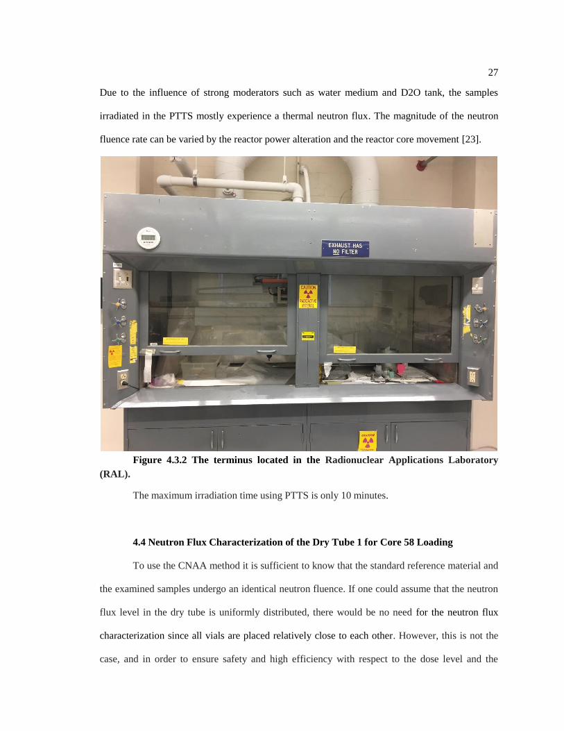
27
Due to the influence of strong moderators such as water medium and D2O tank, the samples
irradiated in the PTTS mostly experience a thermal neutron flux. The magnitude of the neutron
fluence rate can be varied by the reactor power alteration and the reactor core movement [23].
Figure 4.3.2 The terminus located in the Radionuclear Applications Laboratory
(RAL).
The maximum irradiation time using PTTS is only 10 minutes.
4.4 Neutron Flux Characterization of the Dry Tube 1 for Core 58 Loading
To use the CNAA method it is sufficient to know that the standard reference material and
the examined samples undergo an identical neutron fluence. If one could assume that the neutron
flux level in the dry tube is uniformly distributed, there would be no need for the neutron flux
characterization since all vials are placed relatively close to each other. However, this is not the
case, and in order to ensure safety and high efficiency with respect to the dose level and the
28
irradiation time, it is necessary to have accurate data on the magnitude of the neutron flux at
different axial levels along the Dry Tube. The entire experiment was initiated in March of 2018
when the PSBR Core 57 was upgraded to Core 58; thus, the previous neutron flux characterization
was invalid, and a neutron flux measurement with the renewed core pattern had to be implemented.
The flux measurement was conducted mostly following the procedure described in the Master
Thesis of Sarah Sarnoski [23]
The flux of thermal neutrons with energy of 0.0253 eV and resonance (epithermal)
neutrons with energies above 0.5 eV within Dry Tube 1 was measured using an aluminum-gold
wire and 1 mm thick cadmium tubing. These materials were selected due to their specific natural
characteristics. First, the aluminum-gold wire contains 0.112% gold, which absorbs a neutron
through the 197Au(n,γ)198Au reaction. The cross-section values for this reaction ([98.65 ± 0.09 barns]
for thermal neutrons and [1550 ± 28 barns] for resonance neutrons) are high enough that it does not
require a lengthy irradiation [26] In fact, the cross-sections are so large that a high concentration of
gold would produce too much activity. Moreover, the main activation products, such as Al-28, Mg-
27 and Na-24, have half-life periods on the order of minutes to hours, which renders them as short-
lived isotopes compared to the 2.7-day half-life of Au-198. This fact can be used to reduce the
impact of the aluminum alloy on the gamma ray spectrum by extending the time between irradiation
and counting for several days. Finally, the activated isotope of gold (Au-198) returns to a stable
state by emitting a 411.8 keV gamma ray with 98.99% intensity [26].Due to its very large thermal
neutron capture cross section (20615 ± 400 barns) the cadmium tubing was employed as a filter to
determine the resonance neutron flux. [26] Sections of the aluminum-gold wire were sealed in the
cadmium tubing so that only neutrons of epithermal energies are absorbed by the aluminum-gold
wires. The entire procedure of the neutron flux characterization can be described in three main
steps: 1) Preparation of the samples and documentations; 2) Irradiation and counting of the wire
samples; and 3) Analysis of the collected data.

29
4.4.1 Preparation of the samples and documentation
The sample preparation for irradiation commenced with measuring and cutting two 20-inch
and two 3-inch pieces of an aluminum-gold wire. Next, the wires and two aluminum holders for
loading were cleaned with ethanol since the irrelevant elements on the surface might be activated
and contribute to the gamma ray spectrum as trace elements. After cleaning, each item was weighed
using an AE Adams AEA-100SG balance. All these and further actions should be performed using
laboratory gloves, because with direct interaction, human skin can contaminate samples with
sodium and other activatable isotopes. Then, the longest piece was stretched and taped to an
aluminum holder which holds the wire steady and straight. (Note: one end of the tape must be
folded to facilitate its removal from the "hot" wire after irradiation.) The second wire was severed
into six half-inch pieces and placed into 1 mm thick cadmium tubing, which was sealed on both
ends. Further, each of the cadmium covered wires were taped to another aluminum holder following
the pattern shown in Figure 4.4.1.1.
The aluminum holders have marks on the surface with a 1-inch scale, which are useful for
tracking the pattern during the taping. (Note: the cadmium tubing was cut off slightly longer than
half-inch wire to facilitate removal of the wire; thus, the cadmium cover should be taped slightly
below the mark since the alignment occurs over the inner wire and not its cover.) Both bare wire
(BW) and cadmium covered wire (CCW) samples where labeled with DT1 (Dry Tube 1) markings.
The irradiation procedure of the PSBR requires an experiment evaluation and authorization
document called Standard Operating Procedure (SOP-5). This document must include the
experimental description, irradiation conditions and the post-irradiation activity prediction
magnitudes. The latter was performed using an activity prediction application, developed by Dr.
Dağistan Şahin, which will be discussed in detail later in this thesis [25]. Using the information
regarding the type and mass of tested materials, irradiation time, and approximate neutron fluence,
the application estimated the total activity and gamma ray exposure rate with respect to distance

30
and time. Based on the obtained data, was determined the appropriate irradiation time, the decay
time, and the counting time. Finally, the SOP-5 was reviewed and approved by PSBR personnel.
Figure 4.4.1.1. The cadmium covered wire positions within Dry Tube 1 with respect
to fuel rod.
4.4.2 Irradiation and Counting of the Wire Samples
Both sample irradiations were scheduled on Monday mornings when reactor starts after
2.5-day weekend breaks. After that amount of time, the xenon neutron poison (Xe-135)
concentration drastically drops down (half-life is 9.14 hours) making the reactor fresh and ready
for clean critical condition. Under this condition the poison contribution to the neutron fluence will
be minimal, and all control rods will be in near-identical positions. Following the schedule, the first
sample irradiation was initiated on March 19, 2018 at 09:44 AM with a bare wire at the reactor

31
power 800 kW. After 7 minutes of nonstop irradiation, the sample was pulled up to six feet above
the core and remained in Dry Tube 1 to decay for 3 days. Then, it was relocated to the shadow
shield corner and checked by Environmental Health and Safety (EHS) personnel. After getting
EHS authorization to work, the sample was placed into a lead tube container and moved to the
Radionuclear Application Laboratory, which is located on the lower floor of the same building.
(Note: the movement took place utilizing a cart to maintain a safe distance between the human body
and the radioactive sample.) The cadmium covered wire sample was irradiated on the next Monday
at 11:56 AM with the same reactor power and irradiation time. The second sample was also
transported to the laboratory following the identical timing and safety procedures.
In order to determine the actual neutron fluence shape within the Dry Tube 1, the samples
had to be prepared for counting. The objective was to cut the 20-inch activated bare wire into 40
pieces of a half-inch and place each piece into small plastic vial. The objective was accomplished
by pulling the sample out from the container and each time cutting one inch of activated wire by
wire cutter. (Note: after each cutting, the sample should be descended back into container to reduce
radiation exposure. Also, an exposure time can be reduced by using one-inch marks on the
aluminum holder as a measuring tape.) Further, using a long tweezer and wire cutter, each one-inch
piece was cut into two identical pieces in a plexiglass shield box that shield the beta particles
emitted by the wire. Finally, all half-inch pieces were placed into plastic vials and numerated from
1 to 40. Since cutting was started from the top of the wire, number 40 corresponds to the bottom of
the dry tube with respect to the reactor core. The cadmium covered wire was processed utilizing
the same method except for the additional step of removing the aluminum-gold wire from the thin
cadmium tubes. Using pliers, the soft cadmium tubes were squeezed and unsealed which allowed
the wire piece to slip out. Cadmium tubes were later disposed in a container of mixed radioactive
and hazardous waste.

32
The sample counting used an automatic sample changer at the Radiation Science and
Engineering Center, which automates the radioactive counting process, saving working hours, and
providing very consistent measurement times. Each enumerated vial loaded in the sample changer
was automatically picked up and placed into a lead cave with an HPGe detector on the bottom. For
each sample, the live counting time was set to 15 minutes, after which the sample was automatically
retrieved from the cave and placed back in the sample changer wheel. Data acquired from each
sample was automatically saved during the counting process. For both counting sessions, the
detector calibration was not performed since in the Radionuclear Application Laboratory the
detectors are calibrated annually, and during the data acquisition periods the last calibration was
still valid.
4.4.3 Analysis of the Collected Data
Ten days after the irradiation, the vast majority of activated isotopes in the samples
decayed, which made the samples less radioactive. Once the wire pieces were safe to handle, each
wire sample was weighed using an AE Adams AEA-100SG balance. The obtained weight values
were used to determine the number of gold atoms in each sample using Equation (4.4.3.1).
𝑁𝐴𝑢 = 𝑤𝑒𝑖𝑔ℎ𝑡 𝑜𝑓 𝑠𝑎𝑚𝑝𝑙𝑒 ∗𝑊𝐴𝑢 ∗ 𝑁𝐴
𝑀𝐴𝑢 (4.4.3.1)
Where WAu is the gold content in the wire, NA is Avogadro’s number, and MAu is molecular
mass of gold. Due to the isotopic abundance of gold, was assumed that initially 100% of gold
contained Au-197. Considering the relatively low neutron flux magnitude and short irradiation
time, it was also assumed that only a small fraction of gold isotopes was activated, and 100% of
the activated isotopes were Au-198.
In order to calculate the neutron fluence, it is necessary to define the saturation activity. In
theory, the saturation activity can be reached only if the irradiation time is too long in comparison

33
with the half-life of the isotope of interest. Since this is not the case, the saturation activity for each
sample was calculated in a corrected version using Equation (4.4.3.2).
𝐴𝑠𝑎𝑡 = 𝐴𝑚𝑒𝑎𝑠 ∗exp (𝜆 ∙ 𝑡𝑏𝑒𝑡)
(1−exp (−𝜆 ∙ 𝑡𝑖𝑟𝑟𝑎𝑑))∗ 𝜀 (4.4.3.2)
Where 𝐴𝑚𝑒𝑎𝑠 is the measured activity of the wire in counts per second, 𝜆 is the decay
constant of the isotope, 𝑡𝑏𝑒𝑡 is the time between irradiation and counting, 𝑡𝑖𝑟𝑟𝑎𝑑 is the irradiation
time, and 𝜀 is the detector efficiency.
Another valuable variable for calculating the neutron flux is the cadmium ratio (CR), which
is defined as the ratio between the saturation activities of bare and cadmium covered wires located
at the same axial level (Equation 4.4.3.3). The neutron flux within DT1 can be calculated using the
fact that the pieces of BW were irradiated with both thermal and resonance (epithermal) neutrons,
while the CCW pieces were activated by only resonance neutrons.
𝐶𝑅 = 𝐴𝑠𝑎𝑡. 𝐵𝑊
𝐴𝑠𝑎𝑡. 𝐶𝐶𝐷=
𝑡ℎ𝑒𝑟𝑚𝑎𝑙 𝑎𝑐𝑡𝑖𝑣𝑖𝑡𝑦 + 𝑟𝑒𝑠𝑜𝑛𝑎𝑛𝑐𝑒 𝑎𝑐𝑡𝑖𝑣𝑖𝑡𝑦
𝑟𝑒𝑠𝑜𝑛𝑎𝑛𝑐𝑒 𝑎𝑐𝑡𝑖𝑣𝑖𝑡𝑦=
𝐴𝑡ℎ + 𝐴𝑠𝑎𝑡. 𝐶𝐶𝐷
𝐴𝑠𝑎𝑡. 𝐶𝐶𝐷 (4.4.3.3)
Using Equation (4.4.3.3), the CR value was calculated at 5.25”, 8.25”, 11.75”, 13.75”,
16.75”, and 20.25” distances from the DT1 bottom.
To determine the thermal neutron flux within the DT1, it is necessary to define the activity
caused by thermal neutrons. The definition of the thermal activity can be derived from the Equation
(4.4.3.3).
𝐴𝑡ℎ = 𝐴𝑠𝑎𝑡. 𝐶𝐶𝐷 ∗ (𝐶𝑅 − 1) = 𝐴𝑠𝑎𝑡. 𝐵𝑊 ∗ (1 −1
𝐶𝑅) = 𝐴𝑠𝑎𝑡. 𝐵𝑊 ∗ 𝐴𝑅 (4.4.3.4)
Where AR (Activity Ratio) is another consequential variable, which was applied to
facilitate the calculations. Using previously determined CR magnitudes, the AR values were also
computed for six axial positions and plotted in Figure 4.4.3.1. Using a least squares method, the
obtained data was fitted to a first-order polynomial equation (see Figure 4.4.3.1), which further was
used to calculate intermediate AR values for all 40 axial positions. Then, those AR values were
applied to Equation (4.4.3.4) to determine the thermal activity within DT1. As it was planned
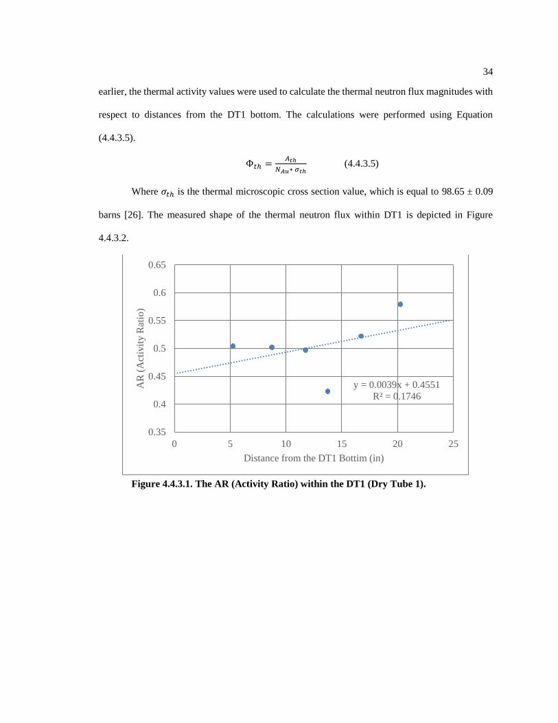
34
earlier, the thermal activity values were used to calculate the thermal neutron flux magnitudes with
respect to distances from the DT1 bottom. The calculations were performed using Equation
(4.4.3.5).
Φ𝑡ℎ =𝐴𝑡ℎ
𝑁𝐴𝑢∗ 𝜎𝑡ℎ (4.4.3.5)
Where 𝜎𝑡ℎ is the thermal microscopic cross section value, which is equal to 98.65 ± 0.09
barns [26]. The measured shape of the thermal neutron flux within DT1 is depicted in Figure
4.4.3.2.
Figure 4.4.3.1. The AR (Activity Ratio) within the DT1 (Dry Tube 1).
y = 0.0039x + 0.4551
R² = 0.1746
0.35
0.4
0.45
0.5
0.55
0.6
0.65
0 5 10 15 20 25
AR
(A
ctiv
ity R
atio
)
Distance from the DT1 Bottim (in)

35
Figure 4.4.3.2. Measured thermal neutron flux within DT1 (Dry Tube 1).
The thermal neutron flux values at each position were used to calculate the true values of
the resonance neutron flux along the DT1. Equation (4.4.3.6) was used for the resonance neutron
flux calculation.
Φ𝑟𝑒𝑠 = (𝐴𝑠𝑎𝑡. 𝐵𝑊
𝑁𝐴𝑢− 𝜎𝑡ℎΦ𝑡ℎ) /𝜎𝑟𝑒𝑠 (4.4.3.6)
Where 𝜎𝑟𝑒𝑠 is the resonance microscopic cross section value, which is equal to 1550 ± 28
barns [26]. In the same way as the thermal neutron flux, the resonance neutron flux was also plotted
as a function of distance from the bottom of the DT1 (see Figure 4.4.3.3).
0.0E+00
2.0E+12
4.0E+12
6.0E+12
8.0E+12
1.0E+13
1.2E+13
0 5 10 15 20 25
Th
erm
al N
eutr
on
Flu
x (
n/c
m^2
*s)
Distance from DT1 Bottom (in)

36
Figure 4.4.3.3. Measured resonance neutron flux within DT1 (Dry Tube 1).
The peak of the thermal neutron flux was at 10.25 inches above the DT1 bottom and
reached a magnitude 1.09x10¹³ n/cm2s. The maximum resonance flux was detected at the same
distance and had a value 7.6x10¹¹ n/cm2s. The average thermal and resonance neutron fluences over
all calculated values were 6.95x10¹² n/cm2s and 4.7x10¹¹ n/cm2s (see Figure 4.4.3.4).
0.0E+00
1.0E+11
2.0E+11
3.0E+11
4.0E+11
5.0E+11
6.0E+11
7.0E+11
8.0E+11
9.0E+11
0 5 10 15 20 25
Res
on
ance
Neu
tro
n F
lux
(n
/cm
^2
*s)
Distance from DT1 Bottom (in)

37
Figure 4.4.3.4. The thermal and resonance neutron flux peak positions within the
DT1 in regard to a PSBR fuel rod.
The error bars demonstrated in Figure 4.4.3.2 and Figure 4.4.3.3 indicate an average of
±5% estimated error. Due to the percentage error, the error magnitudes vary regarding the neutron
flux values. This specific error was chosen based on Hughes’s statement, which claims that the
minimum error for neutron flux determined at a particulate point is ±5% [25] [27]. Moreover, this
error has been used in last neutron fluence measurement experiments executed at PSBR.

38
Chapter 5
Fracking Soil, Sediment and Wastewater Samples
All samples described in this work were obtained from Dr. Nathaniel R. Warner, an
assistant professor of civil and environmental engineering at the Pennsylvania State University.
There were fifteen solid (soil and sediment) and seven liquid (wastewater) samples, placed in
plastic vials of different shapes and properly labeled with the sample name (Figure 5.1). The solid
samples were in the form of differently colored powder or small (1-2 mm) crystals while liquids
were transparent or light-yellow shaded wastewaters.
Figure 5.1. A picture of all tested fracking soil, sediment, and wastewater samples in
their original plastic containers.
Table 5.1 shows a list of characterized fracking samples in this study with a brief
description.
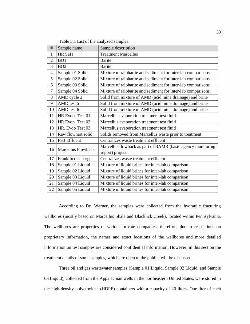
39
Table 5.1 List of the analyzed samples.
# Sample name Sample description
1 HR SaH Treatment Marcellus
2 BO1 Barite
3 BO2 Barite
4 Sample 01 Solid Mixture of raiobarite and sediment for inter-lab comparisons.
5 Sample 02 Solid Mixture of raiobarite and sediment for inter-lab comparisons.
6 Sample 03 Solid Mixture of raiobarite and sediment for inter-lab comparisons.
7 Sample 04 Solid Mixture of raiobarite and sediment for inter-lab comparisons.
8 AMD cycle 2 Solid from mixture of AMD (acid mine drainage) and brine
9 AMD test 5 Solid from mixture of AMD (acid mine drainage) and brine
10 AMD test 6 Solid from mixture of AMD (acid mine drainage) and brine
11 HR Evop. Test 01 Marcellus evaporation treatment test fluid
12 HR Evop. Test 02 Marcellus evaporation treatment test fluid
13 HR, Evop Test 03 Marcellus evaporation treatment test fluid
14 Raw flowhart solid Solids removed from Marcellus waste prior to treatment
15 FS3 Effluent Centralizes waste treatment effluent
16 Marcellus Flowback Marcellus flowback as part of BAMR (basic agency monitoring
report) project
17 Franklin discharge Centralizes waste treatment effluent
18 Sample 01 Liquid Mixture of liquid brines for inter-lab comparison
19 Sample 02 Liquid Mixture of liquid brines for inter-lab comparison
20 Sample 03 Liquid Mixture of liquid brines for inter-lab comparison
21 Sample 04 Liquid Mixture of liquid brines for inter-lab comparison
22 Sample 05 Liquid Mixture of liquid brines for inter-lab comparison
According to Dr. Warner, the samples were collected from the hydraulic fracturing
wellbores (mostly based on Marcellus Shale and Blacklick Creek), located within Pennsylvania.
The wellbores are properties of various private companies; therefore, due to restrictions on
proprietary information, the names and exact locations of the wellbores and more detailed
information on test samples are considered confidential information. However, in this section the
treatment details of some samples, which are open to the public, will be discussed.
Three oil and gas wastewater samples (Sample 01 Liquid, Sample 02 Liquid, and Sample
03 Liquid), collected from the Appalachian wells in the northeastern United States, were stored in
the high-density polyethylene (HDPE) containers with a capacity of 20 liters. One liter of each

40
sample was filtered using a cellulose acetate filter (0.45 µm) and placed in a refrigerator at 4°C for
further analysis of anions, such as Cl, Br, and SO4. Next, after acidifying with 5% HNO3 (nitric
acid), the wastewaters were filtered for cation and radioactivity analyses, such as Al, As, B, Ba, Ca
Cr, Cu, Fe, K, Li, Mg, Mg, Ni, Pb, Ra, Sr, U, and Zn. Then, the sub aliquots of each sample were
placed in HDPE vials and shipped to the laboratories for further analysis [1] The detailed
description on the other liquid samples are not provided..
Four solid samples were pulverized and sieved until they reached a grain size of ~1.18 mm
and had a similar matrix with commonly analyzed solid samples for environmental studies of oil
and gas production impacts, such as barite sludge from treatment facilities, shale core or cuttings,
and river sediments impacted by O&G. In this study, these solid samples labeled as: Sample 01
Solid (a stream sediment collected from the Blacklick Creek, western Pennsylvania), Sample 02
Solid (an outcrop collected from a Marcellus Shale), Sample 03 Solid (the mixture of a stream
sediment from the Blacklick creek with a radio-barite sludge) and Sample 04 Solid (the identical
mixture as Sample 03 Solid, but with different ratio). Before the samples were packed and shipped
to the laboratories, they were homogenized using a concrete mixing paddle [1].

41
Chapter 6
The Experiment
6.1 Activity Prediction
Before any sample irradiation, a system of pre-irradiation activities is required, which
includes activity prediction. At the PSBR, activity prediction is usually performed using the
Activity Predictor program developed by Dr. Dağistan Şahin, a former RSEC graduate student [28].
This tool calculates the expected activity for every isotope in a sample, using input values for the
irradiation location (i.e. the neutron flux), irradiation time, sample mass, and sample elemental
content. In addition, this tool can be used to ensure that the post-irradiation gamma ray dose rate
remains within safety limits. Moreover, it can provide a rough image of the expected gamma ray
spectrum with respect to the decay time. The combination of all this knowledge makes it possible
to improve the experiment design regarding high efficiency, radiation safety, and ideal timing.
The tool was developed using the Java programming language. It calculates activities,
exposure rates, and gamma ray spectra of activated samples using both analytical and Monte Carlo
methods [28]. However, to expedite and simplify the calculation process, the full Monte Carlo
algorithm was substituted with a quasi-version, which can accomplish calculation within minutes.
For calculation, this software uses an XML database that includes the databases such as "Tables
for the analysis of neutron activation" (for neutron cross-section data) [29], Berger and Hubbell’s
XCOM photon cross sections database [30], and Lund/LBNL nuclear data search (for isotope decay
data) [31]. The tool predicts the gamma ray spectrum of the irradiated sample using the efficiency
and geometric characteristics of the HPGe detector located at the Radionuclide Applications
Laboratory (RAL) in RSEC. The tool is user friendly since all desired details regarding reactor,
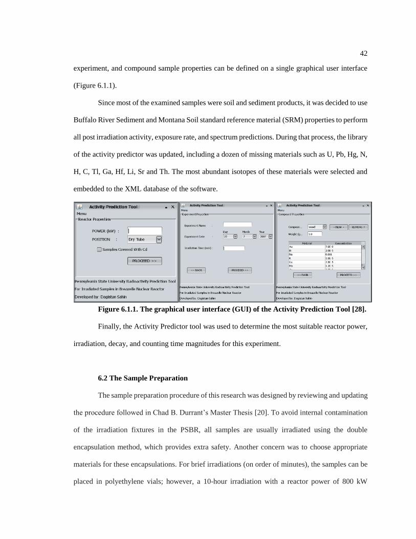
42
experiment, and compound sample properties can be defined on a single graphical user interface
(Figure 6.1.1).
Since most of the examined samples were soil and sediment products, it was decided to use
Buffalo River Sediment and Montana Soil standard reference material (SRM) properties to perform
all post irradiation activity, exposure rate, and spectrum predictions. During that process, the library
of the activity predictor was updated, including a dozen of missing materials such as U, Pb, Hg, N,
H, C, Tl, Ga, Hf, Li, Sr and Th. The most abundant isotopes of these materials were selected and
embedded to the XML database of the software.
Figure 6.1.1. The graphical user interface (GUI) of the Activity Prediction Tool [28].
Finally, the Activity Predictor tool was used to determine the most suitable reactor power,
irradiation, decay, and counting time magnitudes for this experiment.
6.2 The Sample Preparation
The sample preparation procedure of this research was designed by reviewing and updating
the procedure followed in Chad B. Durrant’s Master Thesis [20]. To avoid internal contamination
of the irradiation fixtures in the PSBR, all samples are usually irradiated using the double
encapsulation method, which provides extra safety. Another concern was to choose appropriate
materials for these encapsulations. For brief irradiations (on order of minutes), the samples can be
placed in polyethylene vials; however, a 10-hour irradiation with a reactor power of 800 kW
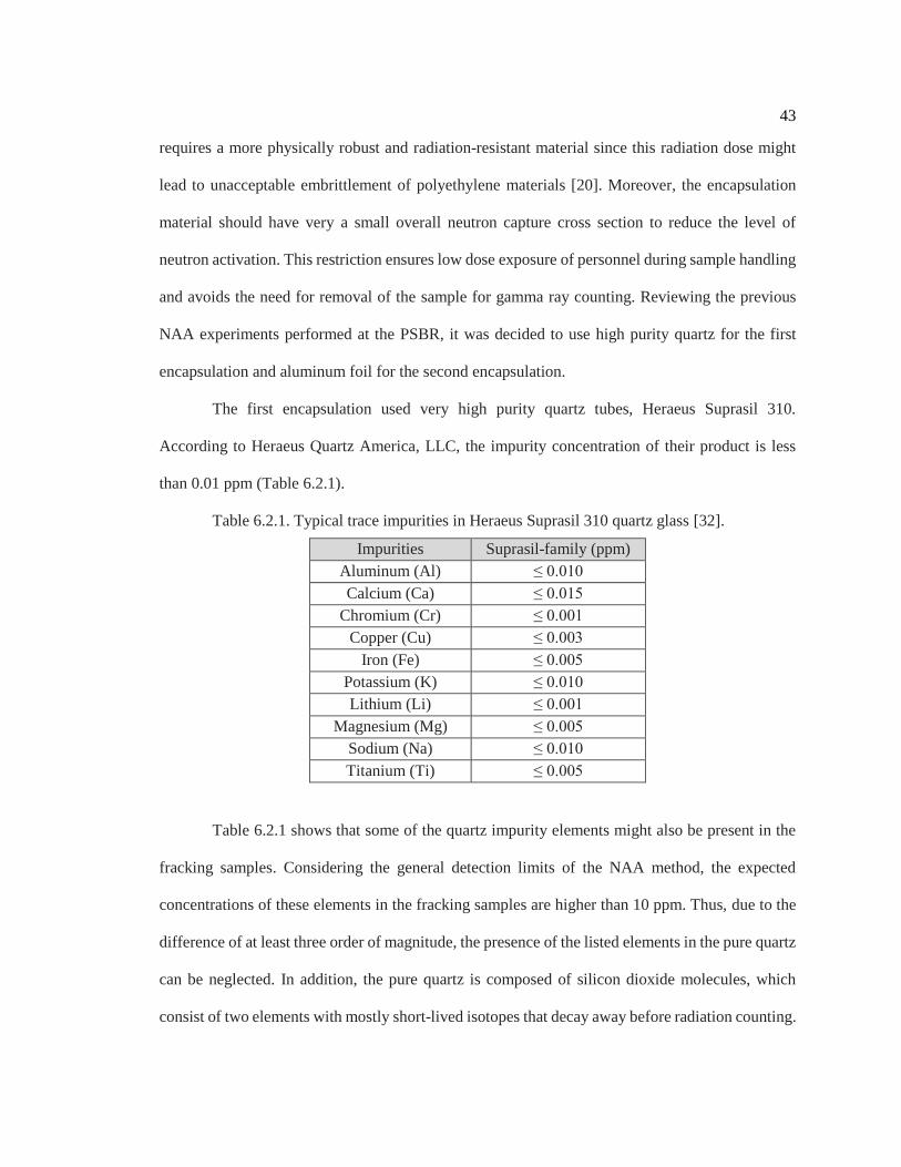
43
requires a more physically robust and radiation-resistant material since this radiation dose might
lead to unacceptable embrittlement of polyethylene materials [20]. Moreover, the encapsulation
material should have very a small overall neutron capture cross section to reduce the level of
neutron activation. This restriction ensures low dose exposure of personnel during sample handling
and avoids the need for removal of the sample for gamma ray counting. Reviewing the previous
NAA experiments performed at the PSBR, it was decided to use high purity quartz for the first
encapsulation and aluminum foil for the second encapsulation.
The first encapsulation used very high purity quartz tubes, Heraeus Suprasil 310.
According to Heraeus Quartz America, LLC, the impurity concentration of their product is less
than 0.01 ppm (Table 6.2.1).
Table 6.2.1. Typical trace impurities in Heraeus Suprasil 310 quartz glass [32].
Impurities Suprasil-family (ppm)
Aluminum (Al) ≤ 0.010
Calcium (Ca) ≤ 0.015
Chromium (Cr) ≤ 0.001
Copper (Cu) ≤ 0.003
Iron (Fe) ≤ 0.005
Potassium (K) ≤ 0.010
Lithium (Li) ≤ 0.001
Magnesium (Mg) ≤ 0.005
Sodium (Na) ≤ 0.010
Titanium (Ti) ≤ 0.005
Table 6.2.1 shows that some of the quartz impurity elements might also be present in the
fracking samples. Considering the general detection limits of the NAA method, the expected
concentrations of these elements in the fracking samples are higher than 10 ppm. Thus, due to the
difference of at least three order of magnitude, the presence of the listed elements in the pure quartz
can be neglected. In addition, the pure quartz is composed of silicon dioxide molecules, which
consist of two elements with mostly short-lived isotopes that decay away before radiation counting.

44
The Heraeus Suprasil 310 quartz tubes are manufactured with a length of 1500 mm, 6 mm
of external and 4 mm of internal diameter. Using a quartz cutting tool, the tubes were cut to ~45
mm pieces. Then, in the machine shop of the RSEC, each quartz tube piece was sealed at one end,
using a propane-oxygen torch. After cooling down, the half-sealed ampoules were cleaned with
ethanol and weighed using the AE Adams AEA-100SG balance. The next step was placing the
SRM, fracking soil and water samples into the ampoules. The SRMs and solid fracking samples
were directly placed into ampoules and numerated for sample identification. (Note: To maintain
high accuracy, it is necessary to clean all used equipment with ethanol and change laboratory gloves
after handling each sample. Also, to avoid scorching of the samples during the top sealing, the top
1 cm of the ampoule should be wiped from the internal dust residue.) Then, the ampoules with
sample containment were initially weighed, dried in a laboratory oven for 2 hours at 110 °C, and
weighed again. After weighing, the dried samples were placed into a desiccator until the open end
of the ampoules were sealed using the identical technique. All weighing records are demonstrated
in Table 6.2.2. The “AMD test 5” and “AMD test 6” solid samples were exception from this general
procedure, since they contained too much water (more information on these samples can be found
in Table 5.1). Thus, they remained in the oven for two days at 110 °C temperature.
Liquid samples contain a high concentration of hydrogen, so to obtain accurate results from
the NAA, they must be dehydrated before irradiation. However, the dehydration process might also
influence the original elemental content of samples by driving off volatile elements such as Se, if
the evaporation temperature is too high. Thus, Dr. Amanda Johnsen and her student Colleen
Mulhollan conducted the research, using Se concentration in a sample. For this research an AAS
(atomic absorption spectroscopy) standard solution was purchased with a selenium concentration
of 1000 µg / ml ± 1% and a molecular formula of Se in 5% HNO3 [33]. Using this solution three
test samples were prepared with a selenium concentration of 10 ppm, 100 ppm, and 1000 ppm
(Figure 6.2.1 (on the left)). Next, these samples were placed into small polyethylene vials, sealed
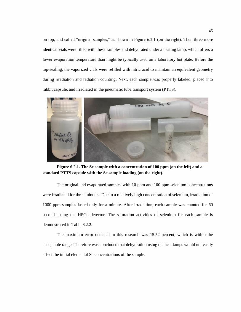
45
on top, and called “original samples,” as shown in Figure 6.2.1 (on the right). Then three more
identical vials were filled with these samples and dehydrated under a heating lamp, which offers a
lower evaporation temperature than might be typically used on a laboratory hot plate. Before the
top-sealing, the vaporized vials were refilled with nitric acid to maintain an equivalent geometry
during irradiation and radiation counting. Next, each sample was properly labeled, placed into
rabbit capsule, and irradiated in the pneumatic tube transport system (PTTS).
Figure 6.2.1. The Se sample with a concentration of 100 ppm (on the left) and a
standard PTTS capsule with the Se sample loading (on the right).
The original and evaporated samples with 10 ppm and 100 ppm selenium concentrations
were irradiated for three minutes. Due to a relatively high concentration of selenium, irradiation of
1000 ppm samples lasted only for a minute. After irradiation, each sample was counted for 60
seconds using the HPGe detector. The saturation activities of selenium for each sample is
demonstrated in Table 6.2.2.
The maximum error detected in this research was 15.52 percent, which is within the
acceptable range. Therefore was concluded that dehydration using the heat lamps would not vastly
affect the initial elemental Se concentrations of the sample.

46
Table 6.2.2. Comparison of selenium saturation activities within original and evaporated
samples.
Concentration Saturation activity (Bq)
Error (%) Original Evaporated
10 ppm 70874.4 59877.5 15.52
100 ppm 690955.5 711527.2 2.98
1000 ppm 6166183.4
6063360.4 1.67
6104804.1 0.99
6107883.1 0.94
Using a measurement pipette, 10 ml of each liquid sample was placed into 20 ml glass vial
and weighed. During the weighing process the fifth digit on the balance screen was continuously
changing every 4-5 seconds, since the balance was sensitive enough to react to evaporation of the
liquid. Consequently, the values shown in Table 6.2.3 might be slightly different from the true mass
values. Next, all glass vials were placed under heating lamp for at least 8 hours until they turned to
solid crystals. After dehydration, the samples were weighted again. The challenge with fifth digit
was faced here too, since the dry crystals were absorbing moisture from the air. Then, the crystals
were powdered and handled as solid samples, following the same procedure. The “Sample 04
liquid” and “Sample 05 liquid” samples have completely evaporated, remaining only a thin layer
of salt on the vial walls. Therefore, those samples were transferred from the vial to the half-ampoule
using distilled water, which later also was evaporated under hitting lamp.

47
Table 6.2.3. The identification numbers and weights of the test samples.
# Sample name Empty ampule (g) Wet mass (mg) Dry mass (mg)
Bucket #1
1 Buffalo River Sediment 1.63443 72.45 72.15
2 Buffalo River Sediment 1.64841 71.7 71.23
3 Montana Soil (2711) 1.69375 72.76 71.5
4 Montana Soil (2711) 1.61128 71.17 70.3
5 HR SaH 1.6334 72.97 68.93
6 BO1 1.62692 73.16 72.84
7 BO2 1.61896 72.47 71.95
8 Sample 01 Solid 1.60217 72.57 72.06
9 Sample 02 Solid 1.57413 71.33 70.74
10 Sample 03 Solid 1.59116 72.62 72.29
11 Sample 04 Solid 1.61689 72.97 72.14
12 AMD cycle 2 1.62174 73.16 70.13
13 AMD test 5 1.64298 74.66 66
14 AMD test 6 1.67561 74.31 65.3
15 HR Evop. Test 01 1.62833 72.58 72.48
16 HR Evop. Test 02 1.59502 72.08 71.93
Bucket #2
1 Buffalo River Sediment 1.67487 69.9 69.23
2 Buffalo River Sediment 1.61928 75.84 75.2
3 Montana Soil (2711) 1.64098 72.58 71.18
4 Montana Soil (2711) 1.6609 73.72 72.11
5 Raw flowhart solid 1.62973 80.48 77.8
6 FS3 Effluent 1.63063 72.73 71.77
7 Marcellus Flowback 1.63067 ------ 94.74
8 Franklin discharge 1.73588 ------ 80.47
9 Sample 01 liquid 1.64267 ------ 84.26
10 Sample 02 liquid 1.66597 ------ 78.79
11 Sample 03 liquid 1.64206 ------ 88.05
12 Sample 04 liquid 1.69295 10.01588 6.93
13 Sample 05 liquid 1.70506 10.0027 6.94
14 HR, Evop. test 03 1.67235 73.62 73.24
In the following Figures 6.2.2 and Figure 6.2.3 all ampullated SRM, soil, sediment and
wastewater samples depicted by bucket and identification numbers.

48
Figure 6.2.2. A picture of fracking and SRM samples placed into Bucket #1.
Figure 6.2.3. A picture of fracking and SRM samples placed into Bucket #2.
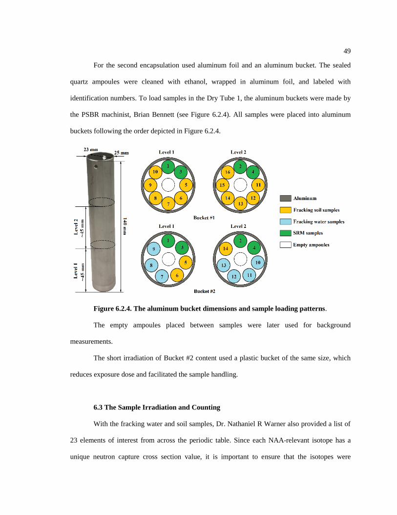
49
For the second encapsulation used aluminum foil and an aluminum bucket. The sealed
quartz ampoules were cleaned with ethanol, wrapped in aluminum foil, and labeled with
identification numbers. To load samples in the Dry Tube 1, the aluminum buckets were made by
the PSBR machinist, Brian Bennett (see Figure 6.2.4). All samples were placed into aluminum
buckets following the order depicted in Figure 6.2.4.
Figure 6.2.4. The aluminum bucket dimensions and sample loading patterns.
The empty ampoules placed between samples were later used for background
measurements.
The short irradiation of Bucket #2 content used a plastic bucket of the same size, which
reduces exposure dose and facilitated the sample handling.
6.3 The Sample Irradiation and Counting
With the fracking water and soil samples, Dr. Nathaniel R Warner also provided a list of
23 elements of interest from across the periodic table. Since each NAA-relevant isotope has a
unique neutron capture cross section value, it is important to ensure that the isotopes were

50
influenced by an adequate neutron flux for a sufficient irradiation time. Moreover, the half-lives of
the product radioisotopes vary from a several minutes to hundreds of days. Therefore, to make the
irradiation and counting more efficient, the list of isotopes was split into three groups, such as short-
lived (T1/2 ≤ 15 hours), intermedium-lived (15 hours < T1/2 < 7 days), and long-lived (T1/2 ≥ 7
days) radioisotopes. The short-lived isotopes can be observed only within a short time frame after
irradiation; thus, to reduce exposure dose of personnel and to safely handle the samples, there is no
need for a long irradiation at high reactor power. Moreover, this allows to avoid detector
overwhelming which causes a tremendous dead time. On the other hand, intermediate- and long-
lived radioisotopes require a long irradiation in the order of hours, since they need to be activated
enough to provide a sufficient number of counts on the gamma ray spectra. After a long irradiation,
the samples should be held for several days before counting. After this decay period, all short-lived
isotopes decay away, which is important for both personnel safety and counting statistics. In other
words, a fewer number of radioactive signals causes a lower Compton continuum, which enables
more accurately identify low-energy gamma photopeaks without being obscured. For these reasons,
the entire irradiation process had to be performed in two stages with short and long periods. The
time for both irradiation periods was determined by reviewing the previous similar work [20] and
the results obtained from the activity predictor. Later, all of the activity prediction information was
documented in the SOP-5 (Standard Operating Procedure), which later was reviewed and approved
by PSBR personnel.
On April 18, 2018 at 9:41 AM was performed the first irradiation, that lasted for 6 minutes
at a reactor power of 110 kW. According to calculations based on irradiation time and known
thermal neutron flux in DT1, the total thermal neutron fluence during the entire irradiation reached
the value of ~7.645x10¹⁴ n/cm2. After irradiation, the aluminum bucket was pulled up and remained
in DT1 for two hours. Then, it was relocated to the shadow shield corner, checked by
Environmental Health and Safety (EHS) personnel, and remained there for another six hours (due
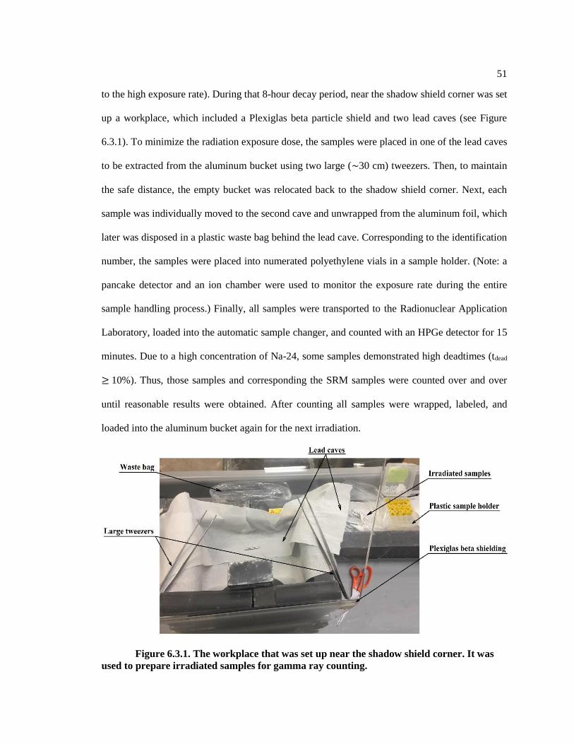
51
to the high exposure rate). During that 8-hour decay period, near the shadow shield corner was set
up a workplace, which included a Plexiglas beta particle shield and two lead caves (see Figure
6.3.1). To minimize the radiation exposure dose, the samples were placed in one of the lead caves
to be extracted from the aluminum bucket using two large (~30 cm) tweezers. Then, to maintain
the safe distance, the empty bucket was relocated back to the shadow shield corner. Next, each
sample was individually moved to the second cave and unwrapped from the aluminum foil, which
later was disposed in a plastic waste bag behind the lead cave. Corresponding to the identification
number, the samples were placed into numerated polyethylene vials in a sample holder. (Note: a
pancake detector and an ion chamber were used to monitor the exposure rate during the entire
sample handling process.) Finally, all samples were transported to the Radionuclear Application
Laboratory, loaded into the automatic sample changer, and counted with an HPGe detector for 15
minutes. Due to a high concentration of Na-24, some samples demonstrated high deadtimes (tdead
≥ 10%). Thus, those samples and corresponding the SRM samples were counted over and over
until reasonable results were obtained. After counting all samples were wrapped, labeled, and
loaded into the aluminum bucket again for the next irradiation.
Figure 6.3.1. The workplace that was set up near the shadow shield corner. It was
used to prepare irradiated samples for gamma ray counting.

52
The long irradiation was triggered on April 24, 2018 and ended at 4:58 PM of the next day,
taking two reactor operation periods. The irradiation was executed at a reactor power of 800 kW
for 10 hours. The irradiation split for two days would not make any difference, since comparators
and unknowns would experience the same exposure and would be analyzed using the CNAA
method. During the entire irradiation the total thermal neutron fluence magnitude was estimated as
~2.5x10¹⁷ n/cm2. After this irradiation the aluminum bucket remained in the DT1 for the five days
until most of the short-lived isotopes decayed. The samples then were prepared for counting,
following the same procedure that was used for the first irradiation. In order to acquire a sufficient
data on gamma-ray signals from intermediate- and long-lived radioisotopes, each sample was
counted for 50 minutes. As predicted, some of the samples demonstrated a very high deadtime
value, so they were recounted after five days with the identical counting time. The next count was
set for 3 hours and was performed when 22 days had elapsed from the day of irradiation. The 3-
hour measurement allowed the collection of an adequate number of counts and facilitated the
identification of the isotope through the gamma-ray spectrum. Due to the high percentage of
deadtime, a 3-hour count was conducted two more times with those particular samples.
Since polyethylene is a sufficiently durable material for short irradiations, it was decided
to replace the aluminum bucket with a polyethylene one with the identical size. This decision allows
to reduce the post-irradiation activity rate and to shorten the decay time between irradiation and
counting. As discussed in section 6.2, most of Bucket #2 content are crystal samples that were
obtained due to dehydration of the liquid samples. Thus, it was assumed that these samples contain
a high concentration of salt elements. Based on this assumption and the information collected from
the first irradiation, it was agreed to decrease the reactor power from 110 kW to 10 kW for the third
irradiation. The third irradiation was started on May 9, 2018 at 8:30 AM and continued for 6
minutes. The total neutron fluence for this irradiation was evaluated as 6.95x10¹³ n/cm2. After
irradiation, the polyethylene bucket with the samples remained in the DT1 for two hours. Then, the

53
Bucket #2 content was prepared for counting in the same manner as previous samples. Each sample
was counted for 15 minutes, after which all samples were again wrapped in aluminum foil and
loaded into the aluminum bucket.
The last irradiation took place within 10 hours at a reactor power of 800 kW. As in the
second exposure, it also lasted for two days and ended May 11, 2018 at 3:43 PM. The fourth
irradiation samples were prepared and counted using the technique and timing that were used for
the samples of the second irradiation.

54
Chapter 7
Experimental Results
7.1 Data Analysis
After collecting all the output gamma spectra from the experiments described in Chapter
6, the data were analyzed using the comparative neutron activation analysis (CNAA) methodology
(Section 3.3.2). Using the information provided by Dr. Nathaniel R Warner regarding the rough
elementary content of the sample matrices, a list of target elements for this study was compiled.
The list includes such elements as Al, B, Na, K, Mg, Ca, Sr, Ba, Cr, Mn, Fe, Ni, Cu, Zn, As, Np
(uranium activation product), Pb, Pa (thorium activation product), Cl, Br, Se, Ag, and Hg. Then,
the corresponding radionuclides of interest were selected for these elements, taking into account
the natural abundance, neutron absorption cross-section, half-life period, and gamma ray emission
intensities and energies. Due to the multiplicity of required characteristics, it was not possible to
determine NAA suitable isotopes for all these elements. For example, Mg-27, Ag-110, Al-28, Br-
80 (very short half-life period), Mg-28, Np-239 (low gamma ray emission energy), Ni-65 (low
natural abundance), Cu-64, Ag-110m (low absolute γ-ray intensity), Pb-209 (no gamma ray
emission), etc. However, after going through all collected gamma ray spectra, there was noticed
the often presence of europium, lanthanum, rubidium, scandium, and cesium isotopes (Figure
7.1.1); thus, it was decided to expand the list of target elements. All target elements and the
corresponding radionuclides are demonstrated in Table 7.1.1, which also contains the gamma-ray
energies used in this research.

55
Table 7.1.1. The list of elements of interest and their radionuclides with gamma-decay
energies used in this study
Element Nuclide Energy (keV)
Chlorine Cl-39 1267.191
Manganese Mn-56 846.764
Europium Eu-152m 841.63
Potassium K-42 1524.6
Sodium Na-24 1368.626
Arsenic As-76 559.1
Lanthanum La-140 1596.21
Calcium Ca-47 1297.06
Barium Ba-131 496.32
Rubidium Rb-86 1077.1
Protactinium Pa-233 311.9
Chromium Cr-51 320.08
Iron Fe-59 1099.24
Mercury Hg-203 279.19
Strontium Sr-85 514.005
Scandium Sc-46 1120.54
Selenium Se-75 264.65
Zinc Zn-65 1115.54
Cesium Cs-134 604.72
The quantitative analysis for these nuclides was performed by using the CNAA method
and certified Buffalo River Sediment concentration values. After determining the concentrations
of trace elements in each sample, the error analysis was conducted via Equation 7.1.1 [20].
𝜎𝜔 = 𝜔√(𝜎𝐴
𝐴)
2+ (
𝜎𝑚
𝑚)
2+ (
𝜎𝑡𝑑
𝑡𝑑)
2 7.1.1.
Where 𝜎𝜔 is the total error or standard deviation of the weight percent, 𝜔 is the
concentration of the element in the sample, A is the measured decay rate, 𝜎𝐴 is the counting
uncertainty obtained from the Genie 2K report, m is the mass of the sample, 𝜎𝑚 is the weighing
error (0.03 mg for the AE Adams AEA-100SG balance), 𝑡𝑑 is the decay time, and 𝜎𝑡𝑑 is the error
associated with decay time (was taken as 60 seconds, due to the uncertainty at the exact (in order
of seconds) end of irradiation time). All calculated values were arranged in tables for each sample,
as shown in Table 7.1.2.

56
Table 7.1.2. Trace element concentrations of Solid 01 Sample.
Element Nuclide Half-life (h) Short
(wt%) Error
Medium
(wt%) Error
Long
(wt%) Error
Chlorine* Cl-39 0.937 3.47E-02 5.86E-03
Manganese Mn-56 2.579 5.93E-02 3.72E-03
Europium Eu-152m 9.312 5.39E-05 2.59E-06
Potassium K-42 12.355 5.50E-01 2.90E-02
Sodium Na-24 14.997 1.19E-01 1.35E-03
Arsenic As-76 26.24 1.98E-03 1.30E-04
Lanthanum La-140 40.285 1.30E-03 1.65E-04 1.28E-03 6.53E-06 1.12E-03 1.75E-04
Calcium Ca-47 108.86 BDL --- BDL ---
Barium Ba-131 276 1.24E-01 2.05E-03 1.01E-01 1.84E-03
Rubidium Rb-86 447.41 3.58E-03 1.42E-04 2.75E-03 9.60E-05
Protactinium Pa-233 647.4 6.68E-04 6.67E-06 4.84E-04 2.81E-06
Chromium Cr-51 664.9 7.52E-03 1.30E-04 1.46E-02 1.82E-04
Iron Fe-59 1067.9 5.50E+00 2.00E-02 7.51E+00 1.65E-02
Mercury Hg-203 1118.3 BDL --- 7.02E-05 8.18E-06
Strontium Sr-85 1556.4 1.74E-01 4.91E-03 1.18E-01 3.07E-03
Scandium Sc-46 2010.9 6.00E-04 2.28E-06 6.03E-04 1.27E-06
Selenium Se-75 2874.7 4.89E-05 2.19E-05 8.95E-05 6.94E-06
Zinc Zn-65 5854.3 7.70E-03 2.39E-04 7.72E-03 1.23E-04
Cesium* Cs-134 18091.1 1.74E-04 7.84E-06 1.72E-04 2.32E-06
The <*> sign in the first column represents non-certified values that have not passed
quality control; also, the BDL stands for below detection limit. The columns <Short>, <Medium>,
and <Long> contain the weight percent magnitude of the element in the first column after decay
period of 8 hours-2 days, 6-12 days, and 22-28 days respectively. The weight percent (wt%) and
can be easily converted to ppm (μg/g), using Equation 7.1.2.
𝑆𝑎𝑚𝑝𝑙𝑒 𝑚𝑎𝑠𝑠 × 𝑤𝑡% × 106 = 𝑝𝑝𝑚 7.1.2
The tables with trace element compositions of other samples can be found in Appendix D. Using
the values from these tables, the trace element concentrations of all fracking solid and liquid
samples were summarized and arranged in two tables (Table 7.1.3 and Table 7.1.4). In these tables
were selected the values with the lowest quality control error (will be discussed in the next
section). Figure 7.1.1. shows an example gamma ray spectrum with labeled gamma ray
photopeaks. The spectrum obtained from the 50-minute counting of Solid 01 Sample with decay
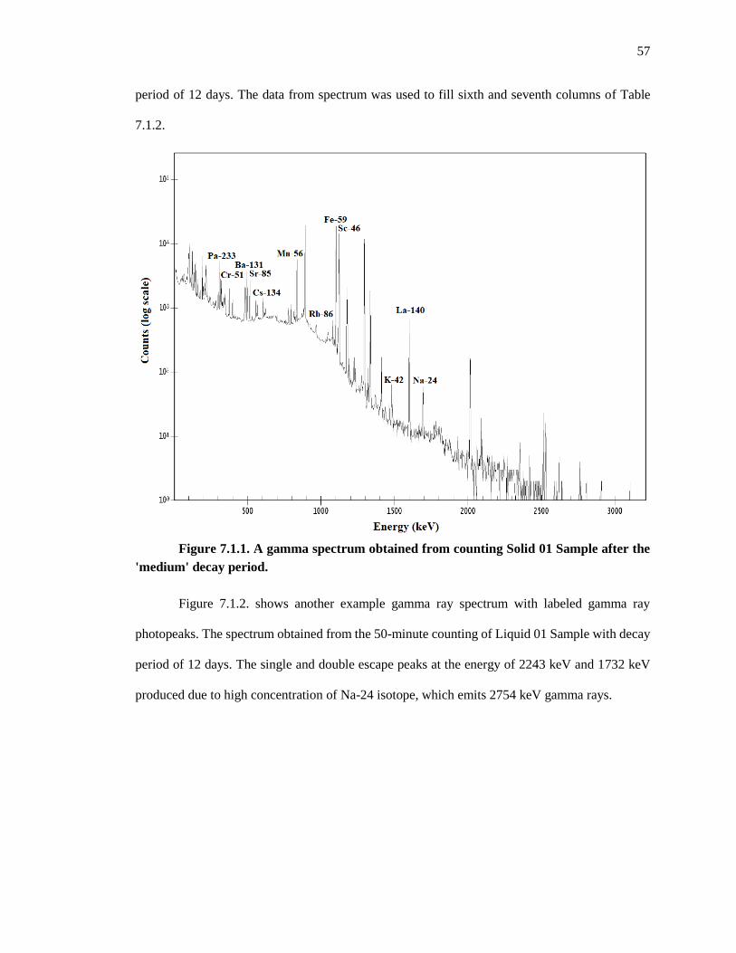
57
period of 12 days. The data from spectrum was used to fill sixth and seventh columns of Table
7.1.2.
Figure 7.1.1. A gamma spectrum obtained from counting Solid 01 Sample after the
'medium' decay period.
Figure 7.1.2. shows another example gamma ray spectrum with labeled gamma ray
photopeaks. The spectrum obtained from the 50-minute counting of Liquid 01 Sample with decay
period of 12 days. The single and double escape peaks at the energy of 2243 keV and 1732 keV
produced due to high concentration of Na-24 isotope, which emits 2754 keV gamma rays.

58
Figure 7.1.2. A gamma spectrum obtained from counting Liquid 01 Sample after the
'medium' decay period.

59
Table 7.1.3. Trace element concentrations of the fracking samples (Part 1). The values are given in weight percent (wt%).
Element Chlorine* Manganese Europium Potassium Sodium Arsenic Lanthanum Calcium Barium
HR SaH BDL BDL BDL 8.94E-02 3.08E+01 4.93E-02 BDL 1.40E+00 7.53E-03
BO1 2.70E-02 1.99E-02 BDL 1.48E-01 1.24E+00 BDL BDL 1.44E+00 4.45E+01
BO2 3.17E-02 5.68E-03 BDL 2.50E-01 1.01E+00 BDL BDL 1.19E+00 4.53E+01
Sample 01 Solid 3.47E-02 5.93E-02 5.39E-05 5.50E-01 1.19E-01 1.98E-03 1.28E-03 BDL 1.24E-01
Sample 02 Solid 4.88E-02 BDL 1.53E-04 1.42E+00 5.21E-02 2.64E-03 2.54E-03 BDL 5.63E-02
Sample 03 Solid 4.97E-02 4.65E-02 6.15E-05 5.67E-01 8.71E-02 1.66E-03 1.49E-03 BDL 4.23E-01
Sample 04 Solid BDL 3.55E-02 9.60E-05 7.04E-01 1.09E-01 1.65E-03 1.77E-03 BDL 1.86E-01
AMD cycle 2 BDL 4.37E-03 BDL 1.34E-01 4.78E+00 BDL BDL 2.98E+00 3.43E+01
AMD test 5 BDL BDL BDL BDL 1.85E+01 BDL BDL 3.58E+00 6.24E+00
AMD test 6 BDL BDL BDL BDL 1.94E+01 BDL BDL 5.62E+00 9.83E+00
HR Evop. Test 01 BDL 2.50E-02 8.34E-06 2.18E-01 6.50E-02 5.51E-03 3.35E-04 1.35E+00 5.86E+01
HR Evop. Test 02 BDL 4.01E-02 1.44E-05 3.02E-01 9.36E-02 5.35E-03 6.00E-04 1.59E+00 5.32E+01
Raw flowhart solid BDL 7.97E-02 BDL 9.23E-01 1.29E+00 3.93E-03 1.02E-03 3.67E+00 3.33E+00
FS3 Effluent 1.34E-03 1.84E-01 BDL 6.35E-01 1.72E+00 BDL 1.46E-03 7.74E+00 5.87E+00
Marcellus Flowback BDL 2.15E-03 BDL 2.46E-02 1.46E+01 5.79E-04 BDL 3.79E+00 2.15E+00
Franklin discharge BDL BDL BDL BDL 1.23E+01 BDL BDL 8.00E+00 7.70E-03
Sample 01 liquid 1.36E-02 4.06E-03 BDL BDL 1.86E+01 BDL BDL 5.60E+00 4.69E-01
Sample 02 liquid BDL 5.51E-03 BDL BDL 1.66E+01 BDL BDL 5.64E+00 5.12E-01
Sample 03 liquid BDL 1.87E-02 BDL 8.01E-01 1.14E+01 BDL BDL 1.04E+01 2.60E-03
Sample 04 liquid 1.12E+00 2.35E-03 BDL 4.17E-01 2.86E+00 BDL 1.29E-04 1.93E+00 3.25E-03
Sample 05 liquid BDL 1.71E-03 BDL BDL 3.32E+00 BDL 6.19E-06 4.48E+00 4.85E-02
HR, Evop test 03 BDL 7.55E-02 BDL BDL 8.09E-01 BDL 1.34E-06 6.83E-01 4.27E+01
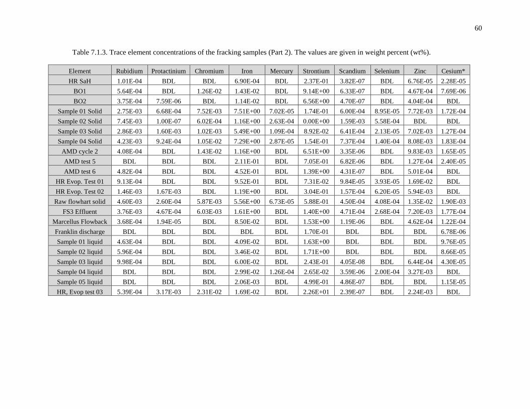
60
Table 7.1.3. Trace element concentrations of the fracking samples (Part 2). The values are given in weight percent (wt%).
Element Rubidium Protactinium Chromium Iron Mercury Strontium Scandium Selenium Zinc Cesium*
HR SaH 1.01E-04 BDL BDL 6.90E-04 BDL 2.37E-01 3.82E-07 BDL 6.76E-05 2.28E-05
BO1 5.64E-04 BDL 1.26E-02 1.43E-02 BDL 9.14E+00 6.33E-07 BDL 4.67E-04 7.69E-06
BO2 3.75E-04 7.59E-06 BDL 1.14E-02 BDL 6.56E+00 4.70E-07 BDL 4.04E-04 BDL
Sample 01 Solid 2.75E-03 6.68E-04 7.52E-03 7.51E+00 7.02E-05 1.74E-01 6.00E-04 8.95E-05 7.72E-03 1.72E-04
Sample 02 Solid 7.45E-03 1.00E-07 6.02E-04 1.16E+00 2.63E-04 0.00E+00 1.59E-03 5.58E-04 BDL BDL
Sample 03 Solid 2.86E-03 1.60E-03 1.02E-03 5.49E+00 1.09E-04 8.92E-02 6.41E-04 2.13E-05 7.02E-03 1.27E-04
Sample 04 Solid 4.23E-03 9.24E-04 1.05E-02 7.29E+00 2.87E-05 1.54E-01 7.37E-04 1.40E-04 8.08E-03 1.83E-04
AMD cycle 2 4.08E-04 BDL 1.43E-02 1.16E+00 BDL 6.51E+00 3.35E-06 BDL 9.83E-03 1.65E-05
AMD test 5 BDL BDL BDL 2.11E-01 BDL 7.05E-01 6.82E-06 BDL 1.27E-04 2.40E-05
AMD test 6 4.82E-04 BDL BDL 4.52E-01 BDL 1.39E+00 4.31E-07 BDL 5.01E-04 BDL
HR Evop. Test 01 9.13E-04 BDL BDL 9.52E-01 BDL 7.31E-02 9.84E-05 3.93E-05 1.69E-02 BDL
HR Evop. Test 02 1.46E-03 1.67E-03 BDL 1.19E+00 BDL 3.04E-01 1.57E-04 6.20E-05 5.94E-03 BDL
Raw flowhart solid 4.60E-03 2.60E-04 5.87E-03 5.56E+00 6.73E-05 5.88E-01 4.50E-04 4.08E-04 1.35E-02 1.90E-03
FS3 Effluent 3.76E-03 4.67E-04 6.03E-03 1.61E+00 BDL 1.40E+00 4.71E-04 2.68E-04 7.20E-03 1.77E-04
Marcellus Flowback 3.68E-04 1.94E-05 BDL 8.50E-02 BDL 1.53E+00 1.19E-06 BDL 4.62E-04 1.22E-04
Franklin discharge BDL BDL BDL BDL BDL 1.70E-01 BDL BDL BDL 6.78E-06
Sample 01 liquid 4.63E-04 BDL BDL 4.09E-02 BDL 1.63E+00 BDL BDL BDL 9.76E-05
Sample 02 liquid 5.96E-04 BDL BDL 3.46E-02 BDL 1.71E+00 BDL BDL BDL 8.66E-05
Sample 03 liquid 9.98E-04 BDL BDL 6.00E-02 BDL 2.43E-01 4.05E-08 BDL 6.44E-04 4.30E-05
Sample 04 liquid BDL BDL BDL 2.99E-02 1.26E-04 2.65E-02 3.59E-06 2.00E-04 3.27E-03 BDL
Sample 05 liquid BDL BDL BDL 2.06E-03 BDL 4.99E-01 4.86E-07 BDL BDL 1.15E-05
HR, Evop test 03 5.39E-04 3.17E-03 2.31E-02 1.69E-02 BDL 2.26E+01 2.39E-07 BDL 2.24E-03 BDL
61
7.2 Quality control
All calculated trace element concentration values need to be checked and verified by
quality control analysis. In this study, quality control was conducted using eight standard reference
samples that contain Buffalo River Sediment and Montana Soil materials. These materials were
certified by National Institute of Standards and Technology (NIST), and their certificates of
analysis are attached to Appendix B. The SRMs were chosen due to similarity in trace element
composition with fracking soil, sediment, and wastewater samples. All elements of interest from
Table 7.1.1 were found in both SRMs, except chlorine that is absent in Montana Soil. Thus, the
chlorine concentration values in each sample did not go through the quality control and were
declared as non-certified.
Both standard reference samples were placed in each level of each bucket and irradiated
with other fracking samples. To perform a more accurate quality control analysis, reference samples
at each level were located as close as possible to each other. In this way, SRMs will be exposed by
the identical neutron fluence, avoiding the spatial neutron flux fluctuation during irradiation. After
irradiation, the SRMs were sequentially counted to minimize any errors that might be caused by a
difference in the decay period. All collected data on the Montana soil SRM were then analyzed in
the same way as fracking sample data. The results were compared to the NIST certified values and
shown in Table 7.2.1 and Table 7.2.2.

62
Table 7.2.1. A summary of quality control analysis for Bucket#1.
Element Nuclide
NIST
value
(wt%)
Measured value
Level 1
(wt%) Error (%)
Level 2
(wt%) Error (%)
Chlorine* Cl-39 --- --- --- --- ---
Manganese Mn-56 6.38E-02 6.95E-02 8.86 5.69E-02 10.78
Europium Eu-152m 1.10E-04 9.54E-05 13.27 1.00E-04 8.91
Potassium K-42 2.45E+00 2.33E+00 5.04 2.45E+00 0.12
Sodium Na-24 1.14E+00 1.03E+00 9.90 1.07E+00 6.42
Arsenic As-76 1.05E-02 1.05E-02 0.26 1.07E-02 1.84
Lanthanum La-140 4.00E-03 4.27E-03 6.68 3.45E-03 13.64
Calcium Ca-47 2.88E+00 3.01E+00 4.38 2.73E+00 5.14
Barium Ba-131 7.26E-02 7.32E-02 0.88 7.19E-02 1.01
Rubidium Rb-86 1.10E-02 1.06E-02 13.52 1.11E-02 0.74
Protactinium Pa-233 1.40E-03 1.24E-03 11.12 1.32E-03 5.40
Chromium Cr-51 4.70E-03 4.39E-03 6.66 4.60E-03 2.03
Iron Fe-59 2.89E+00 3.16E+00 9.46 3.27E-02 6.72
Mercury Hg-203 6.25E-04 6.28E-04 0.52 4.80E-04 23.20
Strontium Sr-85 2.45E-02 2.20E-02 10.47 1.80E-02 26.73
Scandium Sc-46 9.00E-04 9.27E-04 3.05 9.00E-04 0.01
Selenium Se-75 1.52E-04 1.48E-04 2.89 1.63E-04 7.30
Zinc Zn-65 3.50E-02 3.27E-02 6.72 3.28E-02 6.47
Cesium* Cs-134 6.10E-04 --- --- --- ---
Table 7.2.2. A summary of quality control analysis for Bucket#2
Element Nuclide NIST value
(wt%)
Measured value
Level 1
(wt%) Error (%)
Level 2
(wt%) Error (%)
Chlorine* Cl-39 --- --- --- --- ---
Manganese Mn-56 6.38E-02 6.97E-02 9.18 6.68E-02 4.63
Europium Eu-152m 1.10E-04 1.03E-04 6.59 1.10E-04 0.43
Potassium K-42 2.45E+00 2.34E+00 4.36 2.35E+00 3.89
Sodium Na-24 1.14E+00 1.12E+00 1.60 1.06E+00 6.61
Arsenic As-76 1.05E-02 1.63E-02 55.16 8.80E-03 16.22
Lanthanum La-140 4.00E-03 3.55E-03 11.14 3.37E-03 15.78
Calcium Ca-47 2.88E+00 2.91E+00 0.87 3.17E+00 10.16
Barium Ba-131 7.26E-02 6.88E-02 5.24 6.82E-02 6.08
Rubidium Rb-86 1.10E-02 1.15E-02 4.32 1.14E-02 4.05
Protactinium Pa-233 1.40E-03 1.40E-03 0.17 1.40E-03 0.16
Chromium Cr-51 4.70E-03 4.81E-03 2.26 4.72E-03 0.52
Iron Fe-59 2.89E+00 3.02E+00 4.56 2.83E+00 2.25
Mercury Hg-203 6.25E-04 2.66E-04 57.36 BDL ---
Strontium Sr-85 2.45E-02 2.13E-02 13.00 1.03E-02 57.88
Scandium Sc-46 9.00E-04 1.00E-03 11.65 9.41E-04 4.50
Selenium Se-75 1.52E-04 BDL 2.04E-04 34.19
Zinc Zn-65 3.50E-02 3.46E-02 1.12 3.43E-02 2.17
Cesium* Cs-134 6.10E-04 --- --- --- ---

63
Cesium is another non-certified element, since it was not determined in any Montana Soil
gamma ray spectra. Some of these concentration values are significantly different from the NIST
specified concentration values. The concentrations of these elements are extremely small (on the
order of ppm); thus, even small deviation in the ppm range can lead to a significant difference in
the results, which are given in weight percent values. In addition, the NIST certified and
experimentally measured concentration values of each element have the same order of magnitude.
7.3 Interlaboratory Comparison of Results
A study on the accuracy of methods for reporting inorganic element concentrations and
radioactivity in oil and gas wastewaters from the Appalachian Basin was conducted at the Civil &
Environmental Engineering Department of the Pennsylvania State University. Eight academic, six
commercial, and one government laboratories throughout the United States, Canada, and Germany
participated in the study. Each laboratory was instructed to characterize three oil and gas
wastewater samples (Sample 01 Liquid, Sample 02 Liquid, and Sample 03 Liquid) for
concentrations of Cl, Br, S, O, Li, B, Na, K, Mg, Ca, Sr, Ba, Al, Fe, Mn, S, Cr, Ni, Cu, Zn, As, Cd,
and Pb elements. The laboratories that do not have the appropriate equipment or technique to
perform a quantitative analysis on all the elements were allowed to only report within their
capabilities. Also, each laboratory was asked to submit their results to an anonymous online portal
with an attachment of the sample preparation details (dilution factor, precipitation or evaporation
details, etc.), the list of utilized equipment and methodology, uncertainty levels, and calibration
descriptions [1].
The laboratories involved in this study utilized a variety of methods, such as inductively
coupled plasma with optical emission spectrometry (ICP-OES), inductively coupled plasma with
mass spectrometry (ICP-MS), triple quadrupole inductively coupled plasma with mass
spectrometry (ICP-MS/MS), direct current plasma (DCP), X-ray fluorescence (XRF), ion
64
chromatography (IC), and neutron activation analysis (NAA). Some of the commercial laboratories
were previously experienced in analyzing oil and gas wastewater and issued a certificate of analysis
for regulatory applications. Thus, the main objectives of this study were 1) to collect and compare
the trace element concentration values of high salinity oil and gas wastewater, 2) to evaluate the
quality of results of each technique, 2) identify the most suitable application for oil and gas
wastewater characterizations, 4) evaluate the analytical accuracy of detection of target elements
[1].
First, the submitted data were pared down by excluding all zero and below detection limit
values. Then, the numerical values were processed and evaluated using the nonparametric statistical
method that is common for inter-laboratory comparison studies within the United States Geological
Survey (USGS). This method is more resistant to outlier results since it is based not on mean
(average) but, on Quartile 1 (Q1), median, and Quartile 3 (Q3) values. After determining all Q1,
median, and Q3 values for each analyte concertation in each sample, the uncertainty magnitudes
(standard deviation (F-pseudosigma)) were calculated using Equation 7.3.1.
F − pseudosigma =Q3−Q1
1.349 (7.3.1.)
Where 1.349 is a constant that represents the standard deviations necessary to include the
interquartile range data (i.e., Q3-Q1). The median value was claimed as the most probable value
(MPV), in cases where seven or more values were reported per sample and the F-pseudosigma
magnitude was not higher than the median itself. For analytes with only six or five reported values,
the median and F-pseudosigma quantities were evaluated along with the Q1 and Q3 concentration
[1]. Statistical determination was not performed for analytes with less than five reported values and
are marked as not calculable (n.c.) in Table 7.3.1. The most probable value (MPV), F-pseudosigma
(F), lower and upper quartile magnitudes for each analyte are also demonstrated in Table 7.3.1.

65
Table 7.3.1. A summary of inter-laboratory study. All values are represented in mg/l [1].
Analyte Sample 01 Liquid Sample 02 Liquid Sample 03 Liquid
MPV Q1-Q3 F MPV Q1-Q3 F MPV Q1-Q3 F
Br 746 652 - 773 90.4 1270 1180 - 1440 189 1890 1630 - 2060 320
Cl 65600 63900 - 68300 3300 117000 113000 - 120000 5470 176000 160000 - 180000 15000
SO4 n.c. n.c. n.c. n.c. n.c. n.c. 170* 130 – 172* 33.0*
Na 27000 24900 - 28600 2710 47500 43600 - 49300 4260 66850 64600 - 68900 3170
K 336 276 - 383 79.3 716 621 - 765 107 2190 1770 - 2310 402
Mg 1230 1200 - 1300 69.3 2168 2100 - 2270 127 3100 2990 - 3130 104
Ca 10000 9280 - 10200 686 19800 18600 - 20600 1480 31400 30000 - 33200 2350
Sr 2160 2130 - 2200 49.7 3710 3580 - 3940 270 1540 1410 - 1620 156
Ba 659 641 - 690 37.2 1320 1280 - 1380 72.8 6.12 6.07 - 6.33 0.195
Li 32.1 30.3 - 34.3 3 50.3 48 - 51 2.19 71.7 68 - 74.2 4.6
B 5 3.95 - 5.09 0.85 7 6.76 - 8.05 0.95 15.3 14.7 - 16 0.999
Al n.c. n.c. n.c. n.c. n.c. n.c. n.c. n.c. n.c.
Fe 64.8 58.7 - 69 7.61 94.9 85.8 - 98.5 9.44 169 158 - 181 17
Mn 6.1 5.75 - 6.7 0.7 14.4 13.7 - 14.9 0.93 47.8 41.5 - 48.3 5.06
In order to evaluate the performance of the NAA method in the characterization of oil and
gas wastewater samples, the most probable values (MPVs) that obtained from the inter-laboratory
study were compared with NAA measured values (MVs). However, as discussed in Section 7.1,
the NAA method is not applicable to the quantitative analysis of all analytes listed in Table 7.3.1,
therefore the comparison is conducted only among NAA suitable elements. To make the
comparison more convenient, the trace element concentration and standard deviation values were
converted from weight percent (wt%) to milligram per liter (mg/l) and arranged in Table 7.3.2.
Table 7.3.2. The concentration and standard deviation values of some trace elements
measured using the NAA method.
Analyte Sample 01 Liquid Sample 02 Liquid Sample 03 Liquid
MV (mg/l) Error MV (mg/l) Error MV (mg/l) Error
Sodium 24760.8 740.8 39596.5 2059.6 31271.4 1806.3
Potassium BDL --- BDL --- 2203.0 114.7
Calcium 7434.7 348.9 13471.8 670.1 28543.3 1931.5
Strontium 2162.9 51.4 4083.8 95.2 669.3 52.6
Barium 622.4 31.1 1221.8 66.0 7.2 0.9
Iron 54.3 1.4 82.8 5.9 165.1 13.2
Manganese 5.4 0.9 13.1 1.6 51.5 6.5
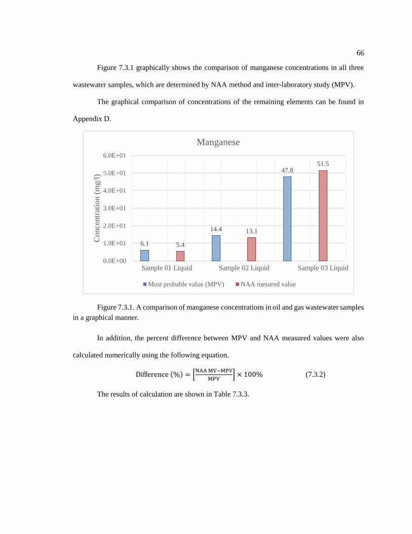
66
Figure 7.3.1 graphically shows the comparison of manganese concentrations in all three
wastewater samples, which are determined by NAA method and inter-laboratory study (MPV).
The graphical comparison of concentrations of the remaining elements can be found in
Appendix D.
Figure 7.3.1. A comparison of manganese concentrations in oil and gas wastewater samples
in a graphical manner.
In addition, the percent difference between MPV and NAA measured values were also
calculated numerically using the following equation.
Difference (%) = [NAA MV−MPV
MPV] × 100% (7.3.2)
The results of calculation are shown in Table 7.3.3.
6.1 5.4
14.4 13.1
47.851.5
0.0E+00
1.0E+01
2.0E+01
3.0E+01
4.0E+01
5.0E+01
6.0E+01
Con
centr
atio
n (
mg/l
)
Sample 01 Liquid Sample 02 Liquid Sample 03 Liquid
Manganese
Most probable value (MPV) NAA mesured value

67
Table 7.3.3. The percent difference magnitudes between MPV and NAA measured
values.
Element Sample 01 Liquid Sample 02 Liquid Sample 03 Liquid
Sodium 8.3 16.6 53.2
Potassium --- --- 0.6
Calcium 25.7 32.0 9.1
Strontium 0.1 10.1 56.5
Barium 5.6 7.4 16.9
Iron 16.1 12.8 2.3
Manganese 11.6 8.7 7.8
If the quality evaluation ranges are set as <20% is acceptable, 20%-40% questionable, and
>40% unacceptable, the NAA provided two questionable (calcium) and two unacceptable
(strontium and sodium) out of 19 values. The barium, iron, and manganese concentration values
agreed with most probable values, since all these elements have the best combination of NAA-
relevant half-time period, relatively high gamma ray energy and intensity.

68
Chapter 8
Conclusion and Future Works
This research determined the multi-elemental characterization of fifteen solid (soil and
sediment) and seven liquid (wastewater) hydraulic fracturing samples collected from wellbores
within Pennsylvania. The characterization was performed using the comparative neutron activation
analysis (CNAA) method for several reasons, such as availability of standard reference materials
(SRM) for comparison, less sensitivity to changes in measurement parameters, similar structure
and geometries of the SRM, powder (soil and sediment), and small crystals (dried wastewater)
samples, as well as less complexity in data analysis. The Buffalo River Sediment and Montana Soil
SRMs obtained from National Institute of Standards and Technology (NIST) were selected as the
standard comparators, since most of the test samples are soil and sediment. In addition, these SRMs
contain almost all of 23 target elements (except chlorine in Montana Soil) for this study, which
includes Al, B, Na, K, Mg, Ca, Sr, Ba, Cr, Mn, Fe, Ni, Cu, Zn, As, Np (uranium activation product),
Pb, Pa (thorium activation product), Cl, Br, Se, Ag, and Hg.
In order to ensure safety and high efficiency with respect to the neutron exposure rate and
time, the neutron flux magnitudes were measures at different axial levels along Dry Tube 1 (DT1)
for the PSBR Core 58 loading. The thermal and resonance (epithermal) neutron flux profiles within
DT1 were determined by irradiating and counting of the bare and cadmium covered aluminum-
gold (0.112% gold) wires. The peak of the thermal and resonance fluxes was determined at 10.25
inches above the DT1 bottom and reached magnitudes of 1.09x10¹³ n/cm2s and 7.6x10¹¹ n/cm2s
respectively.
Further, using the determined neutron flux values, Dr. Dağistan Şahin’s Activity Predictor
program [28] was used to develop an experimental design in terms of sample preparation,

69
irradiation and decay times, and radiation counting durations. All solid fracking samples and SRMs
were weighed, placed into ampoules made from the Heraeus Suprasil 310 quartz tubes, and then
sealed. The liquid samples were dehydrated under the heat lamps until they turned into crystals,
which were subsequently also weighed and encapsulated in the same manner. Such encapsulation
allows to preserve the integrity of the sample matrices after prolonged irradiation and to avoid
internal contamination of the irradiation fixture. Moreover, pure quartz will not be easily activated,
so it negligibly contributes to the total activity of the samples and to the background radiation
during the counting. Then, all samples were placed into two small aluminum buckets following the
pattern shown in Figure 6.2.4. There were two short and two long irradiations conducted for this
research. The short irradiations designed for quantitative analysis of the elements with short-lived
(T1/2 ≤ 15 hours) radionuclides. The short irradiations lasted for 6 minutes at the reactor power of
110 kW and 10 kW with Bucket #1 and Bucket #2 respectively. Long irradiations aimed to analyze
the intermedium-lived (15 hours < T1/2 < 7 days), and long-lived (T1/2 ≥ 7 days) radioisotopes.
Each long irradiation was executed at the reactor power 800 kW for 10 hours. The long irradiations
were split for two reactor operation days, and this fact would not make any difference, since test
samples and comparators would undergo the same neutron fluence and be analyzed using the
CNAA method. To collect data on the short-lived radionuclides, the samples were counted for 15
minutes using the HPGe detector located in a lead cave. Due to high deadtime caused by high
sodium concentrations, the samples were counted in multiple rounds with a range of the decay
period from eight hours to two days. The intermedium-lived radioisotopes were counted for 50
minutes at decay period range of 6-12 days. To acquire a sufficient data on the long-lived
radionuclides, each sample was measured for 3 hours after 22-28 days elapsed from the irradiation.
After collecting gamma ray spectra from all measurements, they were analyzed. The data
analysis started from selecting the NAA suitable isotopes for each target element based on the
natural abundance, neutron absorption cross-section, half-life period, and gamma ray emission

70
intensity and energy characteristics. After this step, the initial list of elements of interest was
reduced to 14 elements, since nine of the desired elements did not have any NAA-relevant isotopes.
During further analysis it was noticed that the photo-peaks with energy corresponding to Eu-152m,
La-140, Rb-86, Sc-46, and Cs-134 isotopes often present in gamma ray spectra of the samples, so
the list of the target elements was updated again. Finally, all samples were analyzed on the
concentration values of 19 trace elements given in Table 7.1.1. After determining the
concentrations of trace elements in each sample, the error analysis was conducted via mass,
measured activity, and decay time uncertainties. The experimentally measured trace element
concentration and error values in weigh percent (wt%) are shown in Tables 7.1.3 and 7.1.4.
Moreover, the elemental concentrations for each individual sample can be found in Table 7.1.2 and
in Appendix D.
To check and verify experimentally measured values, a quality control analysis was
performed using both SRMs. As a result of this analysis, the magnitude of the error in chlorine and
cesium concentrations was not verified, therefore their values were declared non-certified. Arsenic,
mercury, strontium, and selenium demonstrated a high (>20%) percentage of error in certain
measurements (Tables 7.2.1 and 7.2.2). The high error in arsenic concentration is probably
associated with high deadtime. After a short irradiation, the Bucket #2 contents were measured
only once because of the limited time interval caused by the scheduled renovation of the PSBR. In
addition, a high error in selenium concentration can be explained by the lack of irradiation time.
Mercury and strontium may have needed one more counting round with a decay period over 30
days.
Another accuracy check was carried out by comparison of the NAA measured values with
the most probable values (MPV) obtained through inter-laboratory study. In this study participated
15 different laboratories from the US, Canada, and Germany, which used a variety of methods to
determine the trace element concentration of three oil and gas wastewaters. The collected results
71
were evaluated and analyzed using the nonparametric statistical method that allows to identify the
most probable concentration value and approximate standard deviation (Table 7.3.1). According to
the interlaboratory study, the NAA method seems to be provide less accurate results than the
inductively coupled plasma (ICP) method, which traditionally is used for determining trace element
concentrations in oil and gas wastewaters [1]. The comparison of NAA measured values at the
RSEC and the most probable values obtained through inter-laboratory study showed the percent
difference between 0.1% and 56.6%. The relatively large differences in these values might be
caused by several reasons. First, all three samples are liquid wastewaters, which contain a high
concentration of hydride even after the dehydration process. Secondly, due to the evaporation and
absorption of water from the air, it was challenging to weigh both liquid and dried crystalline
samples; thus, the mass error might be high. Thirdly, to avoid a large amount of water absorption,
the crystals were not pulverized, which could cause heterogeneity of the test samples. Finally,
during dehydration, liquid samples were placed from vial to vial, which may lead to a loss of
accuracy.
As the results of this research showed, the NAA and in particular CNAA is a satisfactory
method for conducting quantitative analysis of particular (NAA suitable) elements in the hydraulic
fracturing soil, sediment, and wastewater samples. This technique can be useful as a secondary
analysis to double check results of the prime characterization conducted using the traditional
methods. Moreover, the interlaboratory comparison was conducted for only three liquid samples
and was not the case for any solid samples. Thus, there is a possibility that the NAA may perform
better than other conventional methods in determining the trace element concentrations in fracking
soil and sediments.
Based on the results obtained in this study, the experiment design can be improved for
future work in terms of irradiation, decay, and radiating counting periods. The optimization of the
experiment will reduce detection limits, and subsequently provide more numerical values. Also,
72
the preparation of the liquid samples can be advanced by eliminating mistakes that were made
during the dehydration process in this work.
The range of target elements can be expanded by adding more elements that are typically
challenging for NAA determination. The pneumatic transport system at the Radiation Science and
Engineering Center (RSEC) can be involved to irradiate fracking samples for a short period at low
reactor power, which allows counting samples with short decay period and analyzed very short-
lived radionuclides, such as Mg-27, Br-80, Ag-110, etc. Due to deposition of the partial energy
caused by Compton scattering of gamma rays in the detector, the Compton continuum appears in
the gamma ray spectrum, which obscures most of the low energy photopeaks; thus, it is challenging
to analyze the radioisotopes with lower energy gamma ray emission. However, the Radionuclear
Applications Laboratory (RAL) at the RSEC is equipped with a Compton Suppression System that
reduces the intensity of Compton continuum and more accurately identify the low-energy
photopeaks located within the Compton plateau [23]. This analysis may allow to characterize
radioisotopes such as Mg-28, Np-239, etc.

73
References
[1] Tasker T. L., Burgos B., Ajemigbitse M., Warner N. , "Accuracy of methods for reporting
inorganic element concentrations and radioactivity in oil and gas wastewaters from the
Appalachian Basin, U.S. based on an inter-laboratory comparison," Environmental
Science: Processes and Impacts , 2018.
[2] S. Entrekin, "Rapid expansion of natural gas development poses a threat to surface waters,"
Frontiers in Ecology and the Environment, vol. 9, no. 9, pp. 503-511, 2011.
[3] Q. Meng, S. Ashby, "Distance: A critical aspect for environmental impact assessment of
hydraulic fracking," The Extractive Industries and Society, vol. 1, no. 2, pp. 124-126, 2014.
[4] I. Ferrer, E. Thurman, "Chemical constituents and analytical approaches for hydraulic
fracturing water," Trends in Environmental Analytical Chemistry, vol. 5, pp. 18-25, 2015.
[5] E. R. Adlard, "Michael D. Holloway and Oliver Rudd: Fracking—The Operations and
Environmental Consequences of Hydraulic Fracturing," Chromatographia, vol. 78, no. 7-
8, pp. 601-602, 2015.
[6] Annual Energy Outlook 2014 with projections to 2040, DOE/EIA-0383(2014),
Washington, DC: U.S. Energy Informations Administration (EIA), 2014.
[7] E. Kiviat, "Risks to biodiversity from hydraulic fracturing for natural gas in the Marcellus
and Utica shales," Annals of the New York Academy of Sciences, vol. 1286, no. 1, pp. 1-
14, 2013.
[8] U. D. (. D. o. Energy), "Modern shale gas development in the United States: a primer," in
DC: US DOE. DoE-FG26-04NTl 5455, Washington, 2009.
[9] A. Vengosh, "The Effects of Shale Gas Exploration and Hydraulic Fracturing on the
Quality of Water Resources in the United States," Procedia Earth and Planetary Science,
vol. 7, pp. 863-866, 2013.
[10] K. Ferrar, " Assessment of Effluent Contaminants from Three Facilities Discharging
Marcellus Shale Wastewater to Surface Waters in Pennsylvania," Environmental Science
& Technology, vol. 47, no. 7, pp. 3472-3481, 2013.
[11] E. Barbot, "Spatial and Temporal Correlation of Water Quality Parameters of Produced
Waters from Devonian-Age Shale following Hydraulic Fracturing," Environmental
Science & Technology, vol. 47, no. 6, pp. 2562-2569, 2013.

74
[12] T. Myers, "Potential Contaminant Pathways from Hydraulically Fractured Shale to
Aquifers," Ground Water, vol. 50, no. 6, pp. 872-882, 2012.
[13] E. Chapman, "Geochemical and Strontium Isotope Characterization of Produced Waters
from Marcellus Shale Natural Gas Extraction," Environmental Science & Technology, vol.
46, no. 6, pp. 3545-3553, 2012.
[14] C. C. Wilson, "Radiochemistry and nuclear methods of analysis," Talanta, Vols. 41, (9),
no. ISBN 0-471-30628-2, pp. 1610-1610, 1994.
[15] R. R. Greenberg, P. Bode and De Nadai Fernandes, Elisabete A, "Neutron activation
analysis: A primary method of measurement," Spectrochimica Acta, Vols. 66, (3), no. Part
B: Atomic Spectroscopy, pp. 193-241, 2011.
[16] Lamarsh, J. R., & Baratta, A. J. , Introduction to nuclear engineering, Upper Saddle River,
N.J: Prentice Hal, 2001.
[17] D. K. Hauck, "Dendrochemistry: Seeing the Forest through the Trees," ProQuest
Dissertations Publishing, Vols. 70-11, no. 9781109468861, pp. 71-81, 2009.
[18] M. D. Glascock and H. Neff, "Neutron activation analysis and provenance research in
archaeology," Measurement Science and Technology, Vols. vol. 14, (9), pp. 1516-1526,
2003.
[19] Amanda M. Johnsen, Kenan Ünlü, "Neutron activation analysis capabilities and
applications at the Penn State Radiation Science and Engineering Center," Forensic
Chemistry, vol. 7, pp. 56-64, March 2018.
[20] Chad B. Durrant, "Characterization of Italian Tile Samples Using Comparative Neutron
Activation Analysis in The Penn State Breazeale Nuclear Reactor," M. Sc. thesis in
Mechanical and Nuclear Engineering, Penn State University, State College, May 2014.
[21] A. Simonits, F. De Corte, J. Hoste, "Single-Comparator Methods in Reactor Neutron
Activation Analysis," Journal of Radioanalytical Chemistry, vol. 24, pp. 31-46, 1975.
[22] RSEC, "The Penn State Breazeale Reactor: A Facility for the Past, Present, and Future of
the Pennsylvania State University," PSU, 1993. [Online]. Available:
http://www.rsec.psu.edu/pages/home. [Accessed October 2018].
[23] S. Sarnoski. a. K. Ünlü, "Validation of Performance Measurements of the Penn State
Compton Suppression System," Pennsylvania State University, University Park, 2016.
[24] Danielle Hauck, Kenan Ünlü, "Dendrochemistry: Seeing the forest through the trees,"
Dissertation Abstracts International, Vols. 70-11, pp. 71-81, 2009.

75
[25] D. Şahin, "Activity, Exposure Rate and Gamma Spectrum Prediction for Neutron
irradiated Materials at Radiation Science and Engineering Center," PhD Thesis in Nuclear
Engineering Pennsylvania State University, University Park, State College, PA, December
2008.
[26] International Atomic Energy Agency, "Nuclear Structure and Decay Data," March 2018.
[Online]. Available: www-nds.iaea.org/relnsd/vcharthtml/VChartHTML.html..
[27] D. Hughes, " Pile Neutron Research," Addison-Wesley Publishing Company Inc, 1953.
[28] Sahin, D., & Unlu, K., "Activity, exposure rate and spectrum prediction with java
programming," Journal of Radioanalytical and Nuclear Chemistry, vol. 282(1), no.
doi:10.1007/s10967-009-0316-z, pp. 161-165, 2009.
[29] G. M. (1991), "Tables for Neutron Activation Analysis," The University of Missouri,
Columbia, 1991.
[30] Berger M, Hubbell J, Seltzer S, Chang J, Coursey J, Sukumar R, Zucker D, "XCOM:
photon cross sections database," 1990. [Online]. Available: http:// physics.nist.gov/
PhysRefData/Xcom/Text/XCOM.html.
[31] Chu S, Ekstro¨m L, Firestone R, "Lund/LBNL nuclear data search," 1999. [Online].
Available: http://nucleardata.nuclear.lu.se/nucleardata/toi.
[32] H. Q. Properties, "wilmad-labglass," Heraeus Quartz, [Online]. Available: http://www.
wilmad-labglass.com/uploadedFiles/Main_Site/Pages/Support/Heraeus_Quartz
Properties.pdf.
[33] T. F. Scientific, Alfa Aesar., 2018. [Online]. Available: https://www.alfa.com/en/catalog/
088094/. [Accessed October 2018].
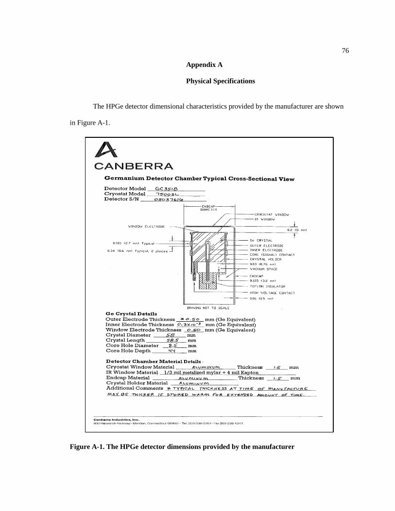
76
Appendix A
Physical Specifications
The HPGe detector dimensional characteristics provided by the manufacturer are shown
in Figure A-1.
Figure A-1. The HPGe detector dimensions provided by the manufacturer
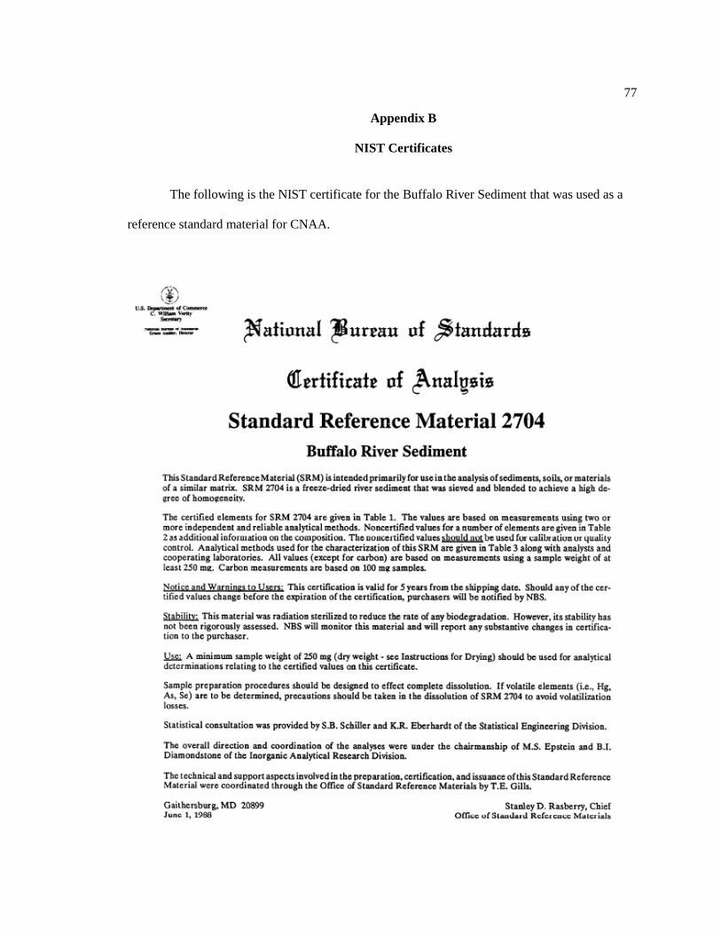
77
Appendix B
NIST Certificates
The following is the NIST certificate for the Buffalo River Sediment that was used as a
reference standard material for CNAA.

78
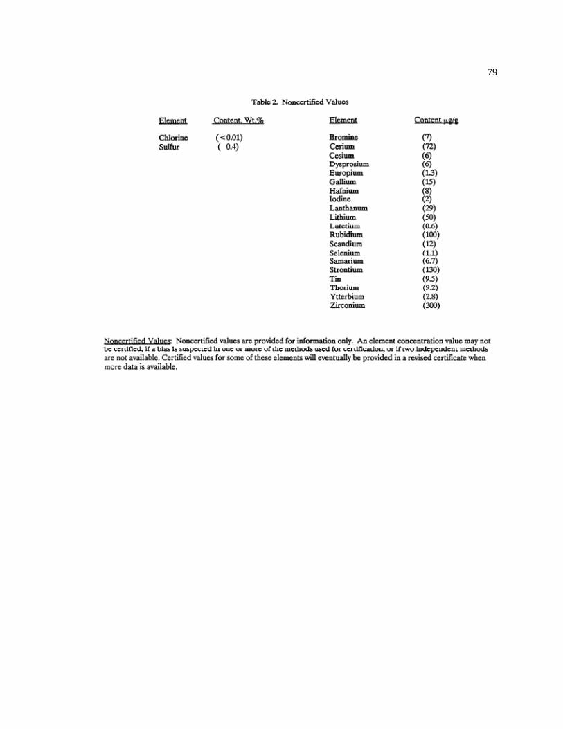
79

80
The following is the NIST certificate for the Montana Soil that was used for the quality
control of the results.
81

82

83

84
Appendix C
Activity Prediction Results
The calculated activity and dose rate values at the end of irradiation are demonstrated in
Tables C-1 through C-4. The values were obtained for Buffalo River Sediment standard reference
material using the Activity Predictor program developed by Dr. Dağistan Şahin. Due to the length
of used tweezers the gamma exposure rate was calculated for 1, 10, and 30 cm distances. The mass
of the sample was given as 0.075 g.
Table C-1. Calculated activities and dose rates for the end of short irradiation of Bucket
#1 content after a decay period of 48 hours.
Isotope Mass (g) Activity (mCi) Gamma Exposure Rate (mrem/hr)
Decay 48 h 1 cm 10 cm 30 cm
Na-24 4.58E-03 5.70E-02 1.61E+04 1.61E+02 1.79E+01
Ca-47 7.80E-08 7.03E-06 3.23E-02 3.23E-04 3.58E-05
Mn-54 1.79E-04 2.04E-06 9.53E-03 9.53E-05 1.06E-05
Cr-51 1.79E-04 1.59E-04 9.79E-02 9.79E-04 1.09E-04
Mn-56 2.83E-03 8.27E-06 6.08E-02 6.08E-04 6.76E-05
Fe-59 8.63E-06 1.58E-04 8.57E-01 8.57E-03 9.52E-04
P-32 7.49E-05 9.92E-04 2.64E+02 2.64E+00 2.93E-01
K-42 1.01E-04 1.76E-02 2.09E+01 2.09E-01 2.32E-02
Si-31 6.76E-04 2.58E-06 4.84E-01 4.84E-03 5.37E-04
Sc-46 2.74E-05 2.22E-04 2.10E+00 2.10E-02 2.33E-03
Sc-47 2.50E-05 5.00E-06 2.33E-03 2.33E-05 2.59E-06
Sc-48 2.53E-04 1.04E-06 1.60E-02 1.60E-04 1.78E-05
Sb-122 1.63E-07 6.75E-05 1.44E-01 1.44E-03 1.60E-04
Sb-124 1.21E-07 2.37E-06 1.92E-02 1.92E-04 2.14E-05
As-76 1.76E-06 8.36E-04 1.53E+00 1.53E-02 1.70E-03
Ba-131 3.29E-08 5.87E-06 1.63E-02 1.63E-04 1.82E-05
Ba-133m 3.14E-08 1.76E-06 6.94E-04 6.94E-06 7.71E-07
Ba-135m 7.50E-07 8.21E-06 4.78E-03 4.78E-05 5.31E-06
Cd-115 7.43E-08 1.32E-06 2.97E-03 2.97E-05 3.30E-06
Co-60 1.05E-06 1.26E-05 1.43E-01 1.43E-03 1.59E-04
Co-58 1.05E-06 1.46E-07 7.69E-04 7.69E-06 8.54E-07
Cu-64 5.12E-06 1.70E-03 2.06E+00 2.06E-02 2.29E-03
Hg-203 3.29E-08 6.01E-07 0.00E+00 0.00E+00 0.00E+00
Zn-65 1.60E-05 2.60E-05 1.23E-01 1.23E-03 1.37E-04
Zn-69m 6.18E-06 3.68E-05 8.08E-02 8.08E-04 8.98E-05
S-35 1.26E-04 3.82E-04 0.00E+00 0.00E+00 0.00E+00
Br-80m 2.66E-07 7.08E-07 4.35E-03 4.35E-05 4.84E-06
Br-82 2.59E-07 7.95E-05 9.92E-01 9.92E-03 1.10E-03
Ce-137 1.03E-08 1.09E-06 6.73E-04 6.73E-06 7.48E-07
Ce-137m 1.03E-08 6.65E-07 3.23E-04 3.23E-06 3.59E-07

85
Ce-141 4.78E-06 2.08E-05 8.10E-03 8.10E-05 9.00E-06
Ce-143 5.98E-07 3.96E-05 6.38E-02 6.38E-04 7.09E-05
Cs-134 4.50E-07 4.96E-06 3.77E-02 3.77E-04 4.18E-05
Dy-165 1.27E-07 4.87E-07 2.08E-05 2.08E-07 2.31E-08
Eu-152 4.66E-08 1.34E-05 6.99E-02 6.99E-04 7.77E-05
Eu-152m 4.66E-08 2.63E-03 3.16E+00 3.16E-02 3.51E-03
Eu-154 5.09E-08 1.18E-06 6.47E-03 6.47E-05 7.19E-06
Ga-72 4.49E-07 5.56E-06 2.27E+00 2.27E-02 2.53E-03
La-140 2.17E-06 1.37E-03 1.37E+01 1.37E-01 1.52E-02
Lu-176m 4.38E-08 1.15E-07 7.02E-06 7.02E-08 7.80E-09
Lu-177 1.17E-09 6.11E-05 9.09E-03 9.09E-05 1.01E-05
Rb-86 5.41E-06 5.59E-05 2.52E-02 2.52E-04 2.80E-05
Se-75 7.43E-10 1.43E-07 2.52E-04 2.52E-06 2.80E-07
Sr-85 5.46E-08 2.33E-07 1.32E-03 1.32E-05 1.47E-06
Sr-89 8.05E-06 3.68E-07 1.60E-07 1.60E-09 1.78E-10
Sm-153 1.34E-07 1.78E-03 7.30E-01 7.30E-03 8.11E-04
Yb-169 2.73E-10 5.88E-06 9.35E-03 9.35E-05 1.04E-05
Yb-175 6.68E-08 3.04E-04 5.66E-02 5.66E-04 6.29E-05
Zr-95 3.91E-06 1.25E-06 4.46E-03 4.46E-05 4.96E-06
Zr-97 6.30E-07 1.05E-06 4.19E-03 4.19E-05 4.65E-06
Table C-1 values were calculated for 6-minute irradiation at the reactor power of 110
kW.
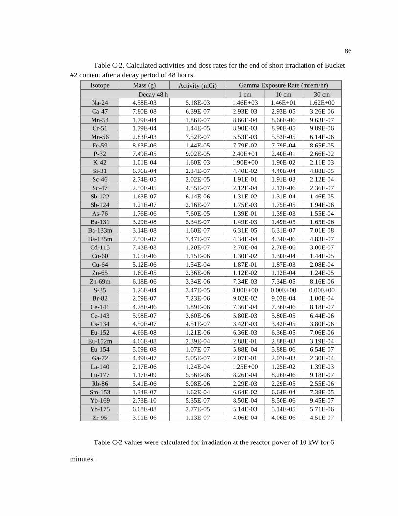
86
Table C-2. Calculated activities and dose rates for the end of short irradiation of Bucket
#2 content after a decay period of 48 hours.
Isotope Mass (g) Activity (mCi) Gamma Exposure Rate (mrem/hr)
Decay 48 h 1 cm 10 cm 30 cm
Na-24 4.58E-03 5.18E-03 1.46E+03 1.46E+01 1.62E+00
Ca-47 7.80E-08 6.39E-07 2.93E-03 2.93E-05 3.26E-06
Mn-54 1.79E-04 1.86E-07 8.66E-04 8.66E-06 9.63E-07
Cr-51 1.79E-04 1.44E-05 8.90E-03 8.90E-05 9.89E-06
Mn-56 2.83E-03 7.52E-07 5.53E-03 5.53E-05 6.14E-06
Fe-59 8.63E-06 1.44E-05 7.79E-02 7.79E-04 8.65E-05
P-32 7.49E-05 9.02E-05 2.40E+01 2.40E-01 2.66E-02
K-42 1.01E-04 1.60E-03 1.90E+00 1.90E-02 2.11E-03
Si-31 6.76E-04 2.34E-07 4.40E-02 4.40E-04 4.88E-05
Sc-46 2.74E-05 2.02E-05 1.91E-01 1.91E-03 2.12E-04
Sc-47 2.50E-05 4.55E-07 2.12E-04 2.12E-06 2.36E-07
Sb-122 1.63E-07 6.14E-06 1.31E-02 1.31E-04 1.46E-05
Sb-124 1.21E-07 2.16E-07 1.75E-03 1.75E-05 1.94E-06
As-76 1.76E-06 7.60E-05 1.39E-01 1.39E-03 1.55E-04
Ba-131 3.29E-08 5.34E-07 1.49E-03 1.49E-05 1.65E-06
Ba-133m 3.14E-08 1.60E-07 6.31E-05 6.31E-07 7.01E-08
Ba-135m 7.50E-07 7.47E-07 4.34E-04 4.34E-06 4.83E-07
Cd-115 7.43E-08 1.20E-07 2.70E-04 2.70E-06 3.00E-07
Co-60 1.05E-06 1.15E-06 1.30E-02 1.30E-04 1.44E-05
Cu-64 5.12E-06 1.54E-04 1.87E-01 1.87E-03 2.08E-04
Zn-65 1.60E-05 2.36E-06 1.12E-02 1.12E-04 1.24E-05
Zn-69m 6.18E-06 3.34E-06 7.34E-03 7.34E-05 8.16E-06
S-35 1.26E-04 3.47E-05 0.00E+00 0.00E+00 0.00E+00
Br-82 2.59E-07 7.23E-06 9.02E-02 9.02E-04 1.00E-04
Ce-141 4.78E-06 1.89E-06 7.36E-04 7.36E-06 8.18E-07
Ce-143 5.98E-07 3.60E-06 5.80E-03 5.80E-05 6.44E-06
Cs-134 4.50E-07 4.51E-07 3.42E-03 3.42E-05 3.80E-06
Eu-152 4.66E-08 1.21E-06 6.36E-03 6.36E-05 7.06E-06
Eu-152m 4.66E-08 2.39E-04 2.88E-01 2.88E-03 3.19E-04
Eu-154 5.09E-08 1.07E-07 5.88E-04 5.88E-06 6.54E-07
Ga-72 4.49E-07 5.05E-07 2.07E-01 2.07E-03 2.30E-04
La-140 2.17E-06 1.24E-04 1.25E+00 1.25E-02 1.39E-03
Lu-177 1.17E-09 5.56E-06 8.26E-04 8.26E-06 9.18E-07
Rb-86 5.41E-06 5.08E-06 2.29E-03 2.29E-05 2.55E-06
Sm-153 1.34E-07 1.62E-04 6.64E-02 6.64E-04 7.38E-05
Yb-169 2.73E-10 5.35E-07 8.50E-04 8.50E-06 9.45E-07
Yb-175 6.68E-08 2.77E-05 5.14E-03 5.14E-05 5.71E-06
Zr-95 3.91E-06 1.13E-07 4.06E-04 4.06E-06 4.51E-07
Table C-2 values were calculated for irradiation at the reactor power of 10 kW for 6
minutes.
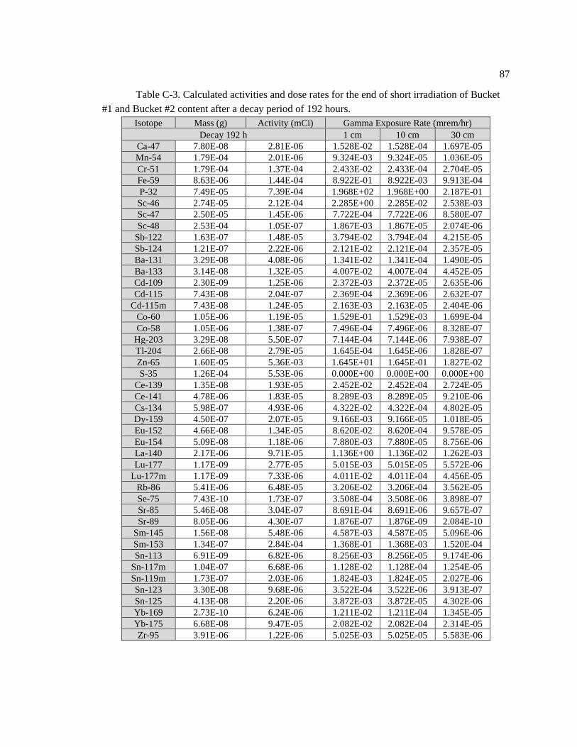
87
Table C-3. Calculated activities and dose rates for the end of short irradiation of Bucket
#1 and Bucket #2 content after a decay period of 192 hours.
Isotope Mass (g) Activity (mCi) Gamma Exposure Rate (mrem/hr)
Decay 192 h 1 cm 10 cm 30 cm
Ca-47 7.80E-08 2.81E-06 1.528E-02 1.528E-04 1.697E-05
Mn-54 1.79E-04 2.01E-06 9.324E-03 9.324E-05 1.036E-05
Cr-51 1.79E-04 1.37E-04 2.433E-02 2.433E-04 2.704E-05
Fe-59 8.63E-06 1.44E-04 8.922E-01 8.922E-03 9.913E-04
P-32 7.49E-05 7.39E-04 1.968E+02 1.968E+00 2.187E-01
Sc-46 2.74E-05 2.12E-04 2.285E+00 2.285E-02 2.538E-03
Sc-47 2.50E-05 1.45E-06 7.722E-04 7.722E-06 8.580E-07
Sc-48 2.53E-04 1.05E-07 1.867E-03 1.867E-05 2.074E-06
Sb-122 1.63E-07 1.48E-05 3.794E-02 3.794E-04 4.215E-05
Sb-124 1.21E-07 2.22E-06 2.121E-02 2.121E-04 2.357E-05
Ba-131 3.29E-08 4.08E-06 1.341E-02 1.341E-04 1.490E-05
Ba-133 3.14E-08 1.32E-05 4.007E-02 4.007E-04 4.452E-05
Cd-109 2.30E-09 1.25E-06 2.372E-03 2.372E-05 2.635E-06
Cd-115 7.43E-08 2.04E-07 2.369E-04 2.369E-06 2.632E-07
Cd-115m 7.43E-08 1.24E-05 2.163E-03 2.163E-05 2.404E-06
Co-60 1.05E-06 1.19E-05 1.529E-01 1.529E-03 1.699E-04
Co-58 1.05E-06 1.38E-07 7.496E-04 7.496E-06 8.328E-07
Hg-203 3.29E-08 5.50E-07 7.144E-04 7.144E-06 7.938E-07
Tl-204 2.66E-08 2.79E-05 1.645E-04 1.645E-06 1.828E-07
Zn-65 1.60E-05 5.36E-03 1.645E+01 1.645E-01 1.827E-02
S-35 1.26E-04 5.53E-06 0.000E+00 0.000E+00 0.000E+00
Ce-139 1.35E-08 1.93E-05 2.452E-02 2.452E-04 2.724E-05
Ce-141 4.78E-06 1.83E-05 8.289E-03 8.289E-05 9.210E-06
Cs-134 5.98E-07 4.93E-06 4.322E-02 4.322E-04 4.802E-05
Dy-159 4.50E-07 2.07E-05 9.166E-03 9.166E-05 1.018E-05
Eu-152 4.66E-08 1.34E-05 8.620E-02 8.620E-04 9.578E-05
Eu-154 5.09E-08 1.18E-06 7.880E-03 7.880E-05 8.756E-06
La-140 2.17E-06 9.71E-05 1.136E+00 1.136E-02 1.262E-03
Lu-177 1.17E-09 2.77E-05 5.015E-03 5.015E-05 5.572E-06
Lu-177m 1.17E-09 7.33E-06 4.011E-02 4.011E-04 4.456E-05
Rb-86 5.41E-06 6.48E-05 3.206E-02 3.206E-04 3.562E-05
Se-75 7.43E-10 1.73E-07 3.508E-04 3.508E-06 3.898E-07
Sr-85 5.46E-08 3.04E-07 8.691E-04 8.691E-06 9.657E-07
Sr-89 8.05E-06 4.30E-07 1.876E-07 1.876E-09 2.084E-10
Sm-145 1.56E-08 5.48E-06 4.587E-03 4.587E-05 5.096E-06
Sm-153 1.34E-07 2.84E-04 1.368E-01 1.368E-03 1.520E-04
Sn-113 6.91E-09 6.82E-06 8.256E-03 8.256E-05 9.174E-06
Sn-117m 1.04E-07 6.68E-06 1.128E-02 1.128E-04 1.254E-05
Sn-119m 1.73E-07 2.03E-06 1.824E-03 1.824E-05 2.027E-06
Sn-123 3.30E-08 9.68E-06 3.522E-04 3.522E-06 3.913E-07
Sn-125 4.13E-08 2.20E-06 3.872E-03 3.872E-05 4.302E-06
Yb-169 2.73E-10 6.24E-06 1.211E-02 1.211E-04 1.345E-05
Yb-175 6.68E-08 9.47E-05 2.082E-02 2.082E-04 2.314E-05
Zr-95 3.91E-06 1.22E-06 5.025E-03 5.025E-05 5.583E-06
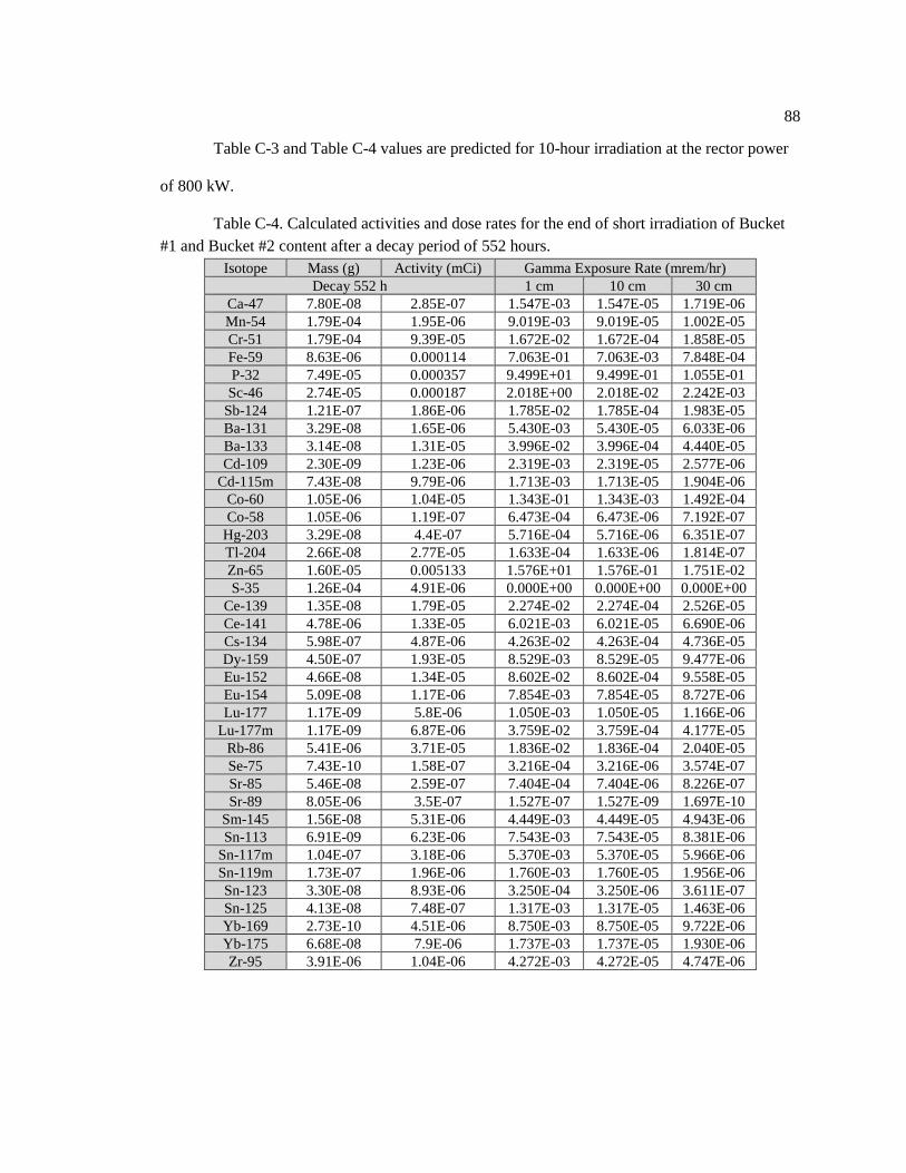
88
Table C-3 and Table C-4 values are predicted for 10-hour irradiation at the rector power
of 800 kW.
Table C-4. Calculated activities and dose rates for the end of short irradiation of Bucket
#1 and Bucket #2 content after a decay period of 552 hours.
Isotope Mass (g) Activity (mCi) Gamma Exposure Rate (mrem/hr)
Decay 552 h 1 cm 10 cm 30 cm
Ca-47 7.80E-08 2.85E-07 1.547E-03 1.547E-05 1.719E-06
Mn-54 1.79E-04 1.95E-06 9.019E-03 9.019E-05 1.002E-05
Cr-51 1.79E-04 9.39E-05 1.672E-02 1.672E-04 1.858E-05
Fe-59 8.63E-06 0.000114 7.063E-01 7.063E-03 7.848E-04
P-32 7.49E-05 0.000357 9.499E+01 9.499E-01 1.055E-01
Sc-46 2.74E-05 0.000187 2.018E+00 2.018E-02 2.242E-03
Sb-124 1.21E-07 1.86E-06 1.785E-02 1.785E-04 1.983E-05
Ba-131 3.29E-08 1.65E-06 5.430E-03 5.430E-05 6.033E-06
Ba-133 3.14E-08 1.31E-05 3.996E-02 3.996E-04 4.440E-05
Cd-109 2.30E-09 1.23E-06 2.319E-03 2.319E-05 2.577E-06
Cd-115m 7.43E-08 9.79E-06 1.713E-03 1.713E-05 1.904E-06
Co-60 1.05E-06 1.04E-05 1.343E-01 1.343E-03 1.492E-04
Co-58 1.05E-06 1.19E-07 6.473E-04 6.473E-06 7.192E-07
Hg-203 3.29E-08 4.4E-07 5.716E-04 5.716E-06 6.351E-07
Tl-204 2.66E-08 2.77E-05 1.633E-04 1.633E-06 1.814E-07
Zn-65 1.60E-05 0.005133 1.576E+01 1.576E-01 1.751E-02
S-35 1.26E-04 4.91E-06 0.000E+00 0.000E+00 0.000E+00
Ce-139 1.35E-08 1.79E-05 2.274E-02 2.274E-04 2.526E-05
Ce-141 4.78E-06 1.33E-05 6.021E-03 6.021E-05 6.690E-06
Cs-134 5.98E-07 4.87E-06 4.263E-02 4.263E-04 4.736E-05
Dy-159 4.50E-07 1.93E-05 8.529E-03 8.529E-05 9.477E-06
Eu-152 4.66E-08 1.34E-05 8.602E-02 8.602E-04 9.558E-05
Eu-154 5.09E-08 1.17E-06 7.854E-03 7.854E-05 8.727E-06
Lu-177 1.17E-09 5.8E-06 1.050E-03 1.050E-05 1.166E-06
Lu-177m 1.17E-09 6.87E-06 3.759E-02 3.759E-04 4.177E-05
Rb-86 5.41E-06 3.71E-05 1.836E-02 1.836E-04 2.040E-05
Se-75 7.43E-10 1.58E-07 3.216E-04 3.216E-06 3.574E-07
Sr-85 5.46E-08 2.59E-07 7.404E-04 7.404E-06 8.226E-07
Sr-89 8.05E-06 3.5E-07 1.527E-07 1.527E-09 1.697E-10
Sm-145 1.56E-08 5.31E-06 4.449E-03 4.449E-05 4.943E-06
Sn-113 6.91E-09 6.23E-06 7.543E-03 7.543E-05 8.381E-06
Sn-117m 1.04E-07 3.18E-06 5.370E-03 5.370E-05 5.966E-06
Sn-119m 1.73E-07 1.96E-06 1.760E-03 1.760E-05 1.956E-06
Sn-123 3.30E-08 8.93E-06 3.250E-04 3.250E-06 3.611E-07
Sn-125 4.13E-08 7.48E-07 1.317E-03 1.317E-05 1.463E-06
Yb-169 2.73E-10 4.51E-06 8.750E-03 8.750E-05 9.722E-06
Yb-175 6.68E-08 7.9E-06 1.737E-03 1.737E-05 1.930E-06
Zr-95 3.91E-06 1.04E-06 4.272E-03 4.272E-05 4.747E-06

89
Appendix D
Analysis Results
The trace element concentrations for each of the tested hydraulic fracturing samples are
shown in Tables D-1 through D-21. The <*> sign in the first column represents non-certified
values that have not passed quality control; also, the BDL stands for below detection limit.
Table D-1. Experimentally determined trace element concentrations of HR SaH sample
using NAA method.
Element Nuclide Half-life
(h)
Short
(wt%) Error
Medium
(wt%) Error
Long
(wt%) Error
Chlorine* Cl-39 0.9367 BDL --- Manganese Mn-56 2.5789 BDL --- Europium Eu-152m 9.3116 BDL --- Potassium K-42 12.355 8.94E-02 1.01E-01 Sodium Na-24 14.997 3.08E+01 3.27E-02 Arsenic As-76 26.24 4.93E-02 5.32E-03
Lanthanum La-140 40.2852 BDL --- BDL --- BDL ---
Calcium Ca-47 108.864 1.40E+00 2.31E-01 1.40E+00 1.01E-01
Barium Ba-131 276 7.53E-03 1.60E-03 7.43E-03 4.44E-04
Rubidium Rb-86 447.408 BDL --- 1.01E-04 2.27E-05
Protactinium Pa-233 647.4 BDL --- BDL ---
Chromium Cr-51 664.896 BDL --- BDL ---
Iron Fe-59 1067.88 BDL --- 6.90E-04 4.23E-04
Mercury Hg-203 1118.26 BDL --- BDL ---
Strontium Sr-85 1556.38 2.37E-01 4.02E-03 2.97E-01 1.88E-03
Scandium Sc-46 2010.96 3.82E-07 2.50E-07 1.32E-07 4.17E-08
Selenium Se-75 2874.72 BDL --- BDL ---
Zinc Zn-65 5854.32 BDL --- 6.76E-05 1.33E-05
Cesium Cs-134 18091.1 BDL --- 2.28E-05 6.13E-07

90
Table D-2. Experimentally determined trace element concentrations of BO1 sample using
NAA method.
Element Nuclide Half-life
(h)
Short
(wt%) Error
Medium
(wt%) Error
Long
(wt%) Error
Chlorine* Cl-39 0.9367 2.70E-02 6.41E-03 Manganese Mn-56 2.5789 1.99E-02 3.62E-02 Europium Eu-152m 9.3116 BDL --- Potassium K-42 12.355 1.48E-01 4.01E-02 Sodium Na-24 14.997 1.24E+00 4.45E-03 Arsenic As-76 26.24 BDL ---
Lanthanum La-140 40.2852 BDL --- BDL --- BDL ---
Calcium Ca-47 108.864 1.44E+00 8.15E-02 1.13E+00 9.41E-02
Barium Ba-131 276 4.45E+01 2.97E-02 4.11E+01 2.43E-02
Rubidium Rb-86 447.408 2.72E-04 3.82E-05 5.64E-04 2.86E-05
Protactinium Pa-233 647.4 BDL --- BDL ---
Chromium Cr-51 664.896 1.65E-02 1.03E-03 1.26E-02 3.72E-04
Iron Fe-59 1067.88 1.28E-02 3.96E-03 1.43E-02 9.86E-04
Mercury Hg-203 1118.26 BDL --- BDL ---
Strontium Sr-85 1556.38 7.75E-00 1.78E-02 9.14E-00 1.06E-02
Scandium Sc-46 2010.96 5.36E-07 1.78E-07 6.33E-07 2.62E-10
Selenium Se-75 2874.72 BDL --- BDL ---
Zinc Zn-65 5854.32 BDL --- 4.67E-05 2.77E-05
Cesium Cs-134 18091.1 3.20E-05 3.71E-06 7.69E-06 1.16E-06
Table D-3. Experimentally determined trace element concentrations of BO2 sample using
NAA method.
Element Nuclide Half-life
(h)
Short
(wt%) Error
Medium
(wt%) Error
Long
(wt%) Error
Chlorine* Cl-39 0.9367 3.17E-02 1.67E-02 Manganese Mn-56 2.5789 5.68E-03 7.68E-03 Europium Eu-152m 9.3116 BDL --- Potassium K-42 12.355 2.50E-01 5.92E-02 Sodium Na-24 14.997 1.01E+00 4.04E-03 Arsenic As-76 26.24 BDL ---
Lanthanum La-140 40.2852 BDL --- BDL --- BDL ---
Calcium Ca-47 108.864 1.19E+00 8.86E-02 1.30E+00 9.69E-02
Barium Ba-131 276 4.53E+01 3.04E-02 4.23E+01 2.51E-02
Rubidium Rb-86 447.408 3.75E-04 4.69E-05 4.30E-04 1.84E-05
Protactinium Pa-233 647.4 BDL --- 7.59E-06 2.35E-08
Chromium Cr-51 664.896 BDL --- BDL ---
Iron Fe-59 1067.88 1.17E-02 1.60E-03 1.14E-02 8.79E-04
Mercury Hg-203 1118.26 BDL --- BDL ---
Strontium Sr-85 1556.38 6.56E+00 1.20E-02 8.10E-00 8.52E-03
Scandium Sc-46 2010.96 4.70E-07 1.29E-07 4.87E-07 5.68E-08
Selenium Se-75 2874.72 BDL --- BDL ---
Zinc Zn-65 5854.32 1.66E-03 9.56E-05 4.04E-04 2.64E-05
Cesium Cs-134 18091.1 BDL --- BDL ---

91
Table D-4. Experimentally determined trace element concentrations of Sample 02 Solid
sample using NAA method.
Element Nuclide Half-life
(h)
Short
(wt%) Error
Medium
(wt%) Error
Long
(wt%) Error
Chlorine* Cl-39 0.9367 4.88E-02 1.03E-02 Manganese Mn-56 2.5789 BDL --- Europium Eu-152m 9.3116 1.53E-04 4.06E-06 Potassium K-42 12.355 1.42E+00 3.63E-02 Sodium Na-24 14.997 5.21E-02 9.37E-04 Arsenic As-76 26.24 2.64E-03 9.58E-05
Lanthanum La-140 40.2852 3.11E-03 1.54E-04 2.54E-03 9.79E-06 1.35E-02 4.10E-04
Calcium Ca-47 108.864 BDL --- BDL ---
Barium Ba-131 276 5.63E-02 2.61E-03 4.85E-02 1.79E-03
Rubidium Rb-86 447.408 7.45E-03 1.55E-04 6.99E-03 9.65E-05
Protactinium Pa-233 647.4 1.00E-07 5.37E-09 5.47E-05 1.06E-06
Chromium Cr-51 664.896 6.02E-04 1.34E-05 1.36E-02 2.14E-04
Iron Fe-59 1067.88 8.09E-01 7.33E-03 1.16E+00 6.02E-03
Mercury Hg-203 1118.26 BDL --- 2.63E-04 2.37E-05
Strontium Sr-85 1556.38 BDL --- BDL ---
Scandium Sc-46 2010.96 1.64E-03 3.81E-06 1.59E-03 2.16E-06
Selenium Se-75 2874.72 2.89E-04 2.24E-05 5.58E-04 2.03E-05
Zinc Zn-65 5854.32 BDL --- BDL ---
Cesium Cs-134 18091.1 BDL --- BDL ---
Table D-5. Experimentally determined trace element concentrations of Sample 03 Solid
sample using NAA method.
Element Nuclide Half-life
(h)
Short
(wt%) Error
Medium
(wt%) Error
Long
(wt%) Error
Chlorine* Cl-39 0.9367 4.97E-02 1.97E-02 Manganese Mn-56 2.5789 4.65E-02 3.53E-03 Europium Eu-152m 9.3116 6.15E-05 2.79E-06 Potassium K-42 12.355 5.67E-01 2.67E-02 Sodium Na-24 14.997 8.71E-02 1.18E-03 Arsenic As-76 26.24 1.66E-03 1.83E-04
Lanthanum La-140 40.2852 1.72E-03 1.52E-04 1.49E-03 7.15E-06 1.69E-03 1.98E-04
Calcium Ca-47 108.864 BDL --- BDL ---
Barium Ba-131 276 5.15E-01 2.41E-03 4.23E-01 2.47E-03
Rubidium Rb-86 447.408 2.86E-03 1.31E-04 2.99E-03 8.79E-05
Protactinium Pa-233 647.4 1.60E-03 1.36E-05 3.98E-04 2.24E-06
Chromium Cr-51 664.896 1.02E-03 2.48E-05 1.73E-02 1.81E-04
Iron Fe-59 1067.88 4.10E+00 1.76E-02 5.49E+00 1.26E-02
Mercury Hg-203 1118.26 BDL --- 1.09E-04 9.73E-06
Strontium Sr-85 1556.38 8.92E-02 3.44E-03 1.25E-01 2.94E-03
Scandium Sc-46 2010.96 6.41E-04 2.35E-06 6.30E-04 1.31E-06
Selenium Se-75 2874.72 2.13E-05 1.41E-05 BDL ---
Zinc Zn-65 5854.32 7.02E-03 2.20E-04 6.67E-03 1.14E-04
Cesium Cs-134 18091.1 1.27E-04 1.08E-06 1.43E-04 1.98E-06
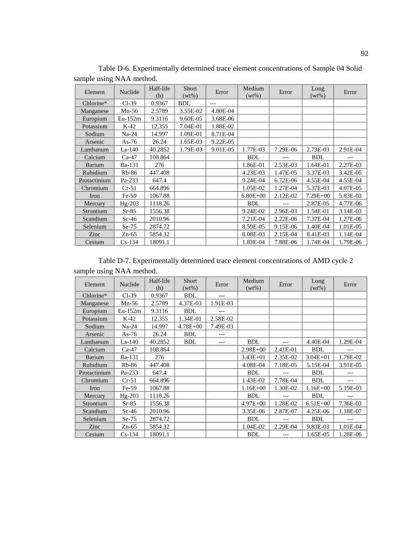
92
Table D-6. Experimentally determined trace element concentrations of Sample 04 Solid
sample using NAA method.
Element Nuclide Half-life
(h)
Short
(wt%) Error
Medium
(wt%) Error
Long
(wt%) Error
Chlorine* Cl-39 0.9367 BDL --- Manganese Mn-56 2.5789 3.55E-02 4.80E-04 Europium Eu-152m 9.3116 9.60E-05 3.68E-06 Potassium K-42 12.355 7.04E-01 1.88E-02 Sodium Na-24 14.997 1.09E-01 8.71E-04 Arsenic As-76 26.24 1.65E-03 9.22E-05
Lanthanum La-140 40.2852 1.79E-03 9.01E-05 1.77E-03 7.29E-06 2.73E-03 2.91E-04
Calcium Ca-47 108.864 BDL --- BDL ---
Barium Ba-131 276 1.86E-01 2.53E-03 1.64E-01 2.27E-03
Rubidium Rb-86 447.408 4.23E-03 1.47E-05 3.37E-03 3.42E-05
Protactinium Pa-233 647.4 9.24E-04 6.72E-06 4.55E-04 4.55E-04
Chromium Cr-51 664.896 1.05E-02 1.27E-04 5.37E-03 4.07E-05
Iron Fe-59 1067.88 6.80E+00 2.12E-02 7.29E+00 5.83E-03
Mercury Hg-203 1118.26 BDL --- 2.87E-05 4.77E-06
Strontium Sr-85 1556.38 9.24E-02 2.96E-03 1.54E-01 3.14E-03
Scandium Sc-46 2010.96 7.21E-04 2.22E-06 7.37E-04 1.27E-06
Selenium Se-75 2874.72 8.59E-05 9.15E-06 1.40E-04 1.01E-05
Zinc Zn-65 5854.32 8.08E-03 2.15E-04 8.41E-03 1.14E-04
Cesium Cs-134 18091.1 1.83E-04 7.88E-06 1.74E-04 1.79E-06
Table D-7. Experimentally determined trace element concentrations of AMD cycle 2
sample using NAA method.
Element Nuclide Half-life
(h)
Short
(wt%) Error
Medium
(wt%) Error
Long
(wt%) Error
Chlorine* Cl-39 0.9367 BDL --- Manganese Mn-56 2.5789 4.37E-03 1.91E-03 Europium Eu-152m 9.3116 BDL --- Potassium K-42 12.355 1.34E-01 2.58E-02 Sodium Na-24 14.997 4.78E+00 7.49E-03 Arsenic As-76 26.24 BDL ---
Lanthanum La-140 40.2852 BDL --- BDL --- 4.40E-04 1.29E-04
Calcium Ca-47 108.864 2.98E+00 2.41E-01 BDL ---
Barium Ba-131 276 3.43E+01 2.35E-02 3.04E+01 1.78E-02
Rubidium Rb-86 447.408 4.08E-04 7.18E-05 5.15E-04 3.91E-05
Protactinium Pa-233 647.4 BDL --- BDL ---
Chromium Cr-51 664.896 1.43E-02 7.78E-04 BDL ---
Iron Fe-59 1067.88 1.16E+00 1.30E-02 1.16E+00 5.19E-03
Mercury Hg-203 1118.26 BDL --- BDL ---
Strontium Sr-85 1556.38 4.97E+00 1.28E-02 6.51E+00 7.36E-03
Scandium Sc-46 2010.96 3.35E-06 2.87E-07 4.25E-06 1.18E-07
Selenium Se-75 2874.72 BDL --- BDL ---
Zinc Zn-65 5854.32 1.04E-02 2.29E-04 9.83E-03 1.01E-04
Cesium Cs-134 18091.1 BDL --- 1.65E-05 1.28E-06
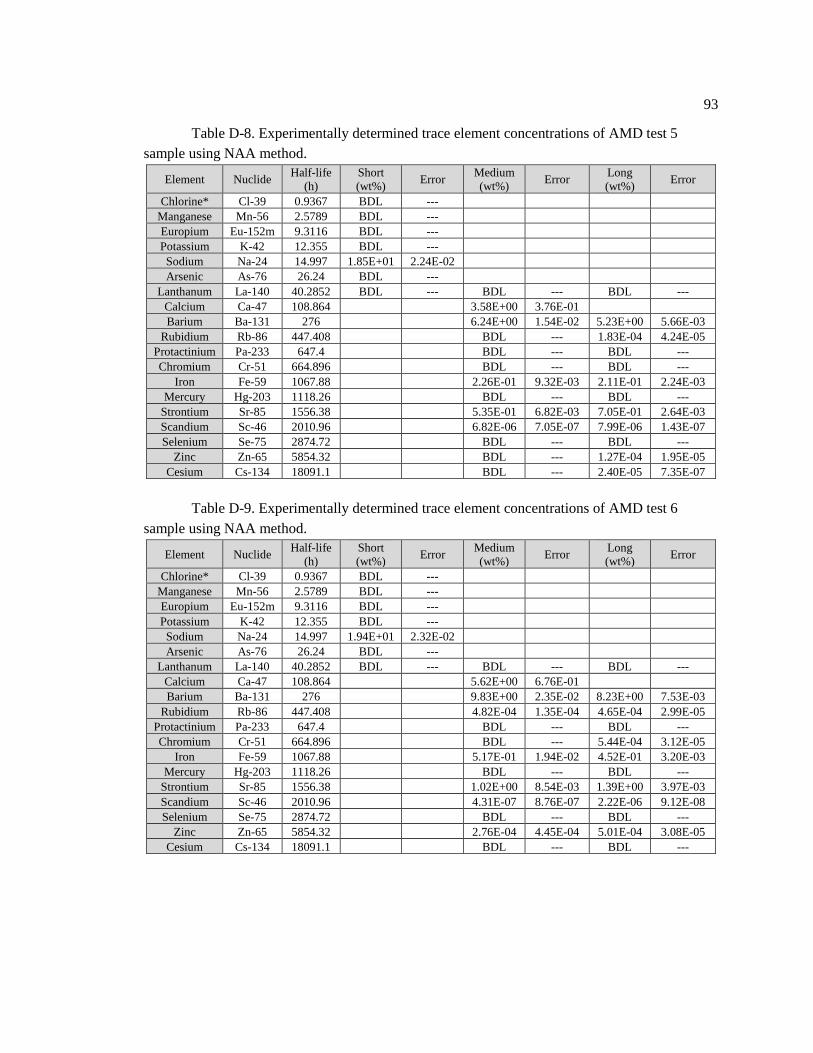
93
Table D-8. Experimentally determined trace element concentrations of AMD test 5
sample using NAA method.
Element Nuclide Half-life
(h)
Short
(wt%) Error
Medium
(wt%) Error
Long
(wt%) Error
Chlorine* Cl-39 0.9367 BDL --- Manganese Mn-56 2.5789 BDL --- Europium Eu-152m 9.3116 BDL --- Potassium K-42 12.355 BDL --- Sodium Na-24 14.997 1.85E+01 2.24E-02 Arsenic As-76 26.24 BDL ---
Lanthanum La-140 40.2852 BDL --- BDL --- BDL ---
Calcium Ca-47 108.864 3.58E+00 3.76E-01 Barium Ba-131 276 6.24E+00 1.54E-02 5.23E+00 5.66E-03
Rubidium Rb-86 447.408 BDL --- 1.83E-04 4.24E-05
Protactinium Pa-233 647.4 BDL --- BDL ---
Chromium Cr-51 664.896 BDL --- BDL ---
Iron Fe-59 1067.88 2.26E-01 9.32E-03 2.11E-01 2.24E-03
Mercury Hg-203 1118.26 BDL --- BDL ---
Strontium Sr-85 1556.38 5.35E-01 6.82E-03 7.05E-01 2.64E-03
Scandium Sc-46 2010.96 6.82E-06 7.05E-07 7.99E-06 1.43E-07
Selenium Se-75 2874.72 BDL --- BDL ---
Zinc Zn-65 5854.32 BDL --- 1.27E-04 1.95E-05
Cesium Cs-134 18091.1 BDL --- 2.40E-05 7.35E-07
Table D-9. Experimentally determined trace element concentrations of AMD test 6
sample using NAA method.
Element Nuclide Half-life
(h)
Short
(wt%) Error
Medium
(wt%) Error
Long
(wt%) Error
Chlorine* Cl-39 0.9367 BDL --- Manganese Mn-56 2.5789 BDL --- Europium Eu-152m 9.3116 BDL --- Potassium K-42 12.355 BDL --- Sodium Na-24 14.997 1.94E+01 2.32E-02 Arsenic As-76 26.24 BDL ---
Lanthanum La-140 40.2852 BDL --- BDL --- BDL ---
Calcium Ca-47 108.864 5.62E+00 6.76E-01
Barium Ba-131 276 9.83E+00 2.35E-02 8.23E+00 7.53E-03
Rubidium Rb-86 447.408 4.82E-04 1.35E-04 4.65E-04 2.99E-05
Protactinium Pa-233 647.4 BDL --- BDL ---
Chromium Cr-51 664.896 BDL --- 5.44E-04 3.12E-05
Iron Fe-59 1067.88 5.17E-01 1.94E-02 4.52E-01 3.20E-03
Mercury Hg-203 1118.26 BDL --- BDL ---
Strontium Sr-85 1556.38 1.02E+00 8.54E-03 1.39E+00 3.97E-03
Scandium Sc-46 2010.96 4.31E-07 8.76E-07 2.22E-06 9.12E-08
Selenium Se-75 2874.72 BDL --- BDL ---
Zinc Zn-65 5854.32 2.76E-04 4.45E-04 5.01E-04 3.08E-05
Cesium Cs-134 18091.1 BDL --- BDL ---
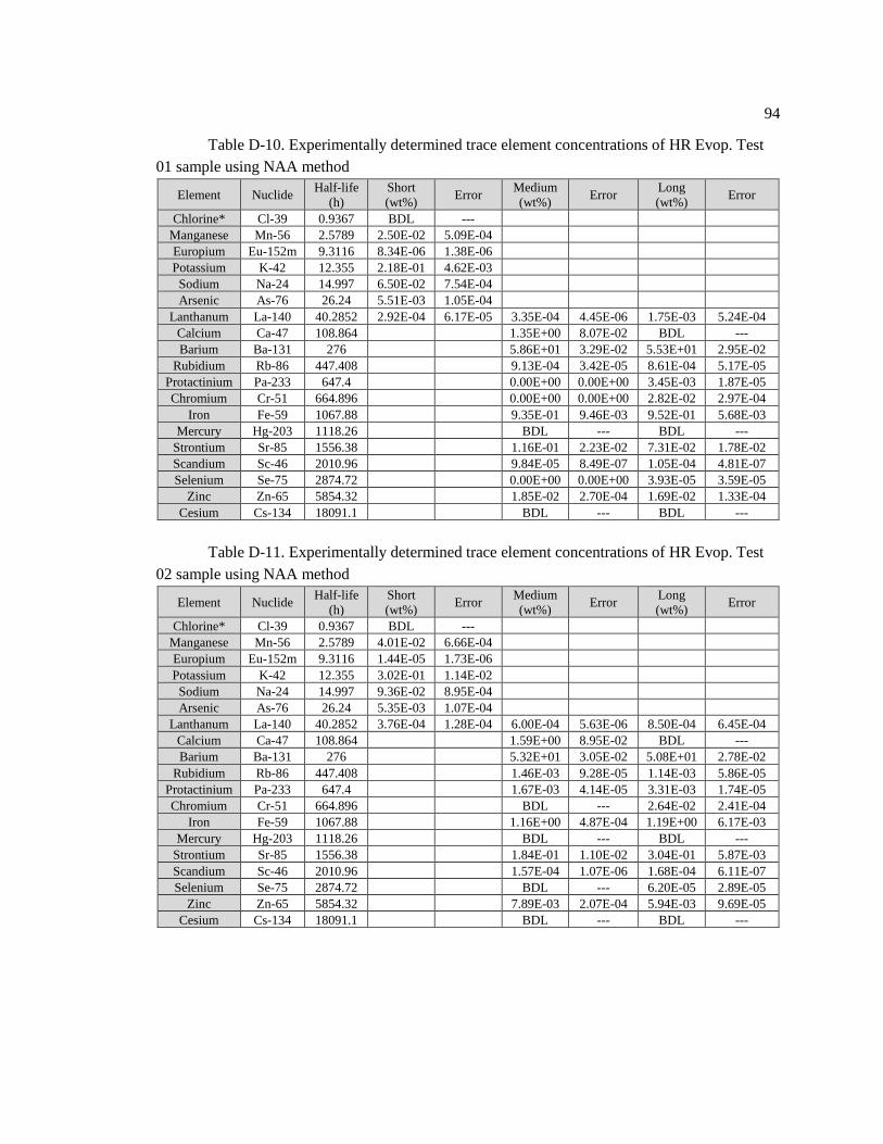
94
Table D-10. Experimentally determined trace element concentrations of HR Evop. Test
01 sample using NAA method
Element Nuclide Half-life
(h)
Short
(wt%) Error
Medium
(wt%) Error
Long
(wt%) Error
Chlorine* Cl-39 0.9367 BDL --- Manganese Mn-56 2.5789 2.50E-02 5.09E-04 Europium Eu-152m 9.3116 8.34E-06 1.38E-06 Potassium K-42 12.355 2.18E-01 4.62E-03 Sodium Na-24 14.997 6.50E-02 7.54E-04 Arsenic As-76 26.24 5.51E-03 1.05E-04
Lanthanum La-140 40.2852 2.92E-04 6.17E-05 3.35E-04 4.45E-06 1.75E-03 5.24E-04
Calcium Ca-47 108.864 1.35E+00 8.07E-02 BDL ---
Barium Ba-131 276 5.86E+01 3.29E-02 5.53E+01 2.95E-02
Rubidium Rb-86 447.408 9.13E-04 3.42E-05 8.61E-04 5.17E-05
Protactinium Pa-233 647.4 0.00E+00 0.00E+00 3.45E-03 1.87E-05
Chromium Cr-51 664.896 0.00E+00 0.00E+00 2.82E-02 2.97E-04
Iron Fe-59 1067.88 9.35E-01 9.46E-03 9.52E-01 5.68E-03
Mercury Hg-203 1118.26 BDL --- BDL ---
Strontium Sr-85 1556.38 1.16E-01 2.23E-02 7.31E-02 1.78E-02
Scandium Sc-46 2010.96 9.84E-05 8.49E-07 1.05E-04 4.81E-07
Selenium Se-75 2874.72 0.00E+00 0.00E+00 3.93E-05 3.59E-05
Zinc Zn-65 5854.32 1.85E-02 2.70E-04 1.69E-02 1.33E-04
Cesium Cs-134 18091.1 BDL --- BDL ---
Table D-11. Experimentally determined trace element concentrations of HR Evop. Test
02 sample using NAA method
Element Nuclide Half-life
(h)
Short
(wt%) Error
Medium
(wt%) Error
Long
(wt%) Error
Chlorine* Cl-39 0.9367 BDL --- Manganese Mn-56 2.5789 4.01E-02 6.66E-04 Europium Eu-152m 9.3116 1.44E-05 1.73E-06 Potassium K-42 12.355 3.02E-01 1.14E-02 Sodium Na-24 14.997 9.36E-02 8.95E-04 Arsenic As-76 26.24 5.35E-03 1.07E-04
Lanthanum La-140 40.2852 3.76E-04 1.28E-04 6.00E-04 5.63E-06 8.50E-04 6.45E-04
Calcium Ca-47 108.864 1.59E+00 8.95E-02 BDL ---
Barium Ba-131 276 5.32E+01 3.05E-02 5.08E+01 2.78E-02
Rubidium Rb-86 447.408 1.46E-03 9.28E-05 1.14E-03 5.86E-05
Protactinium Pa-233 647.4 1.67E-03 4.14E-05 3.31E-03 1.74E-05
Chromium Cr-51 664.896 BDL --- 2.64E-02 2.41E-04
Iron Fe-59 1067.88 1.16E+00 4.87E-04 1.19E+00 6.17E-03
Mercury Hg-203 1118.26 BDL --- BDL ---
Strontium Sr-85 1556.38 1.84E-01 1.10E-02 3.04E-01 5.87E-03
Scandium Sc-46 2010.96 1.57E-04 1.07E-06 1.68E-04 6.11E-07
Selenium Se-75 2874.72 BDL --- 6.20E-05 2.89E-05
Zinc Zn-65 5854.32 7.89E-03 2.07E-04 5.94E-03 9.69E-05
Cesium Cs-134 18091.1 BDL --- BDL ---

95
Table D-12. Experimentally determined trace element concentrations of Raw flowhart
solid sample using NAA method
Element Nuclide Half-life
(h)
Short
(wt%) Error
Medium
(wt%) Error
Long
(wt%) Error
Chlorine* Cl-39 0.9367 BDL ---
Manganese Mn-56 2.5789 7.97E-02 4.95E-04
Europium Eu-152m 9.3116 BDL ---
Potassium K-42 12.355 9.23E-01 6.55E-02
Sodium Na-24 14.997 1.29E+00 9.21E-03
Arsenic As-76 26.24 3.93E-03 9.69E-04
Lanthanum La-140 40.2852 1.02E-03 5.81E-06 3.92E-03 3.20E-04
Calcium Ca-47 108.864 3.67E+00 2.12E-01 3.20E+00 2.81E-01
Barium Ba-131 276 3.33E+00 6.72E-03 3.17E+00 4.97E-03
Rubidium Rb-86 447.408 4.60E-03 1.55E-04 5.29E-03 1.01E-04
Protactinium Pa-233 647.4 2.60E-04 8.17E-06 2.23E-05 9.00E-07
Chromium Cr-51 664.896 5.87E-03 1.38E-04 1.12E-02 8.71E-05
Iron Fe-59 1067.88 5.56E+00 2.52E-02 5.67E+00 1.33E-02
Mercury Hg-203 1118.26 BDL --- 6.73E-05 1.41E-05
Strontium Sr-85 1556.38 8.10E-01 1.39E-02 5.88E-01 4.56E-03
Scandium Sc-46 2010.96 4.50E-04 1.96E-06 4.79E-04 1.15E-06
Selenium Se-75 2874.72 BDL --- 4.08E-04 6.80E-05
Zinc Zn-65 5854.32 1.35E-02 6.30E-04 BDL ---
Cesium Cs-134 18091.1 1.75E-03 1.40E-05 1.90E-03 7.99E-06
Table D-13. Experimentally determined trace element concentrations of FS3 Effluent
sample using NAA method
Element Nuclide Half-life
(h)
Short
(wt%) Error
Medium
(wt%) Error
Long
(wt%) Error
Chlorine* Cl-39 0.9367 1.34E-03 1.62E-02
Manganese Mn-56 2.5789 1.84E-01 8.87E-04
Europium Eu-152m 9.3116 BDL ---
Potassium K-42 12.355 6.35E-01 7.45E-02
Sodium Na-24 14.997 1.72E+00 1.16E-02
Arsenic As-76 26.24 BDL ---
Lanthanum La-140 40.2852 1.46E-03 7.12E-06 1.81E-03 1.83E-04
Calcium Ca-47 108.864 7.74E+00 2.80E-01 6.90E+00 1.55E-01
Barium Ba-131 276 5.87E+00 8.53E-03 5.23E+00 5.96E-03
Rubidium Rb-86 447.408 3.76E-03 1.30E-04 3.67E-03 7.44E-05
Protactinium Pa-233 647.4 4.67E-04 8.82E-06 9.30E-04 5.88E-06
Chromium Cr-51 664.896 6.03E-03 1.38E-04 5.36E-04 2.20E-05
Iron Fe-59 1067.88 1.61E+00 1.55E-02 1.59E+00 6.47E-03
Mercury Hg-203 1118.26 BDL --- BDL ---
Strontium Sr-85 1556.38 1.96E+00 1.49E-02 1.40E+00 5.08E-03
Scandium Sc-46 2010.96 4.39E-04 1.99E-06 4.71E-04 1.18E-06
Selenium Se-75 2874.72 BDL --- 2.68E-04 2.75E-04
Zinc Zn-65 5854.32 7.46E-03 5.51E-04 7.20E-03 1.08E-04
Cesium Cs-134 18091.1 2.14E-04 8.93E-06 1.77E-04 1.87E-06

96
Table D-14. Experimentally determined trace element concentrations of Marcellus
Flowback sample using NAA method
Element Nuclide Half-life
(h)
Short
(wt%) Error
Medium
(wt%) Error
Long
(wt%) Error
Chlorine* Cl-39 0.9367 BDL ---
Manganese Mn-56 2.5789 2.15E-03 3.74E-04
Europium Eu-152m 9.3116 BDL ---
Potassium K-42 12.355 2.46E-02 9.67E-02
Sodium Na-24 14.997 1.46E+01 4.66E-02
Arsenic As-76 26.24 5.79E-04 3.88E-03
Lanthanum La-140 40.2852 BDL --- BDL ---
Calcium Ca-47 108.864 3.79E+00 2.30E-01 3.50E+00 1.54E-01
Barium Ba-131 276 2.15E+00 4.28E-03 1.93E+00 2.94E-03
Rubidium Rb-86 447.408 3.68E-04 1.44E-04 5.11E-04 3.41E-05
Protactinium Pa-233 647.4 1.94E-05 6.59E-06 BDL ---
Chromium Cr-51 664.896 BDL --- BDL ---
Iron Fe-59 1067.88 8.50E-02 6.03E-03 8.64E-02 1.37E-03
Mercury Hg-203 1118.26 BDL --- BDL ---
Strontium Sr-85 1556.38 1.53E+00 9.66E-03 1.04E+00 3.00E-03
Scandium Sc-46 2010.96 1.50E-06 3.39E-07 1.19E-06 6.53E-08
Selenium Se-75 2874.72 BDL --- BDL ---
Zinc Zn-65 5854.32 N/A N/A 4.62E-04 2.90E-05
Cesium Cs-134 18091.1 1.06E-04 3.79E-06 1.22E-04 1.15E-06
Table D-15. Experimentally determined trace element concentrations Franklin discharge
sample using NAA method
Element Nuclide Half-life
(h)
Short
(wt%) Error
Medium
(wt%) Error
Long
(wt%) Error
Chlorine* Cl-39 0.9367 BDL ---
Manganese Mn-56 2.5789 BDL ---
Europium Eu-152m 9.3116 BDL ---
Potassium K-42 12.355 BDL ---
Sodium Na-24 14.997 1.23E+01 5.21E-02
Arsenic As-76 26.24 BDL ---
Lanthanum La-140 40.2852 BDL --- BDL ---
Calcium Ca-47 108.864 8.00E+00 2.74E-01 5.65E+00 1.36E-01
Barium Ba-131 276 7.70E-03 3.69E-03 4.01E-03 2.66E-04
Rubidium Rb-86 447.408 BDL --- 1.85E-04 3.00E-05
Protactinium Pa-233 647.4 BDL --- BDL ---
Chromium Cr-51 664.896 BDL --- BDL ---
Iron Fe-59 1067.88 BDL --- BDL ---
Mercury Hg-203 1118.26 BDL --- BDL ---
Strontium Sr-85 1556.38 1.25E-01 1.99E-02 1.70E-01 1.58E-03
Scandium Sc-46 2010.96 BDL --- BDL ---
Selenium Se-75 2874.72 BDL --- BDL ---
Zinc Zn-65 5854.32 BDL --- BDL ---
Cesium Cs-134 18091.1 BDL --- 6.78E-06 5.06E-07

97
Table D-16. Experimentally determined trace element concentrations Sample 01 liquid
sample using NAA method
Element Nuclide Half-life
(h)
Short
(wt%) Error
Medium
(wt%) Error
Long
(wt%) Error
Chlorine* Cl-39 0.9367 1.36E-02 8.99E-02
Manganese Mn-56 2.5789 4.06E-03 6.59E-04
Europium Eu-152m 9.3116 BDL ---
Potassium K-42 12.355 BDL ---
Sodium Na-24 14.997 1.86E+01 5.58E-01
Arsenic As-76 26.24 BDL ---
Lanthanum La-140 40.2852 BDL --- BDL ---
Calcium Ca-47 108.864 5.60E+00 2.63E-01 4.25E+00 1.70E-01
Barium Ba-131 276 4.69E-01 2.34E-02 4.17E-01 1.48E-02
Rubidium Rb-86 447.408 4.63E-04 1.55E-04 7.30E-04 2.98E-05
Protactinium Pa-233 647.4 BDL --- BDL ---
Chromium Cr-51 664.896 BDL --- BDL ---
Iron Fe-59 1067.88 3.53E-02 7.09E-03 4.09E-02 1.08E-03
Mercury Hg-203 1118.26 BDL --- BDL ---
Strontium Sr-85 1556.38 2.35E+00 1.14E-02 1.63E+00 3.87E-02
Scandium Sc-46 2010.96 BDL --- BDL ---
Selenium Se-75 2874.72 BDL --- BDL ---
Zinc Zn-65 5854.32 BDL --- BDL ---
Cesium Cs-134 18091.1 8.94E-05 2.13E-06 9.76E-05 1.07E-06
Table D-17. Experimentally determined trace element concentrations Sample 02 liquid
sample using NAA method
Element Nuclide Half-life
(h)
Short
(wt%) Error
Medium
(wt%) Error
Long
(wt%) Error
Chlorine* Cl-39 0.9367 BDL ---
Manganese Mn-56 2.5789 5.51E-03 6.85E-04
Europium Eu-152m 9.3116 BDL ---
Potassium K-42 12.355 BDL ---
Sodium Na-24 14.997 1.66E+01 8.62E-01
Arsenic As-76 26.24 BDL ---
Lanthanum La-140 40.2852 BDL --- BDL ---
Calcium Ca-47 108.864 5.64E+00 2.81E-01 3.96E+00 1.36E-01
Barium Ba-131 276 5.12E-01 2.76E-02 4.05E-01 1.53E-02
Rubidium Rb-86 447.408 5.96E-04 8.02E-05 6.92E-04 2.34E-05
Protactinium Pa-233 647.4 BDL --- BDL ---
Chromium Cr-51 664.896 BDL --- 2.17E-04 3.39E-05
Iron Fe-59 1067.88 3.46E-02 2.47E-03 3.91E-02 1.19E-03
Mercury Hg-203 1118.26 BDL --- BDL ---
Strontium Sr-85 1556.38 2.55E+00 1.14E-01 1.71E+00 3.99E-02
Scandium Sc-46 2010.96 BDL --- BDL ---
Selenium Se-75 2874.72 BDL --- BDL ---
Zinc Zn-65 5854.32 BDL --- BDL ---
Cesium Cs-134 18091.1 7.65E-05 2.01E-06 8.66E-05 1.10E-06

98
Table D-18. Experimentally determined trace element concentrations Sample 03 liquid
sample using NAA method
Element Nuclide Half-life
(h)
Short
(wt%) Error
Medium
(wt%) Error
Long
(wt%) Error
Chlorine* Cl-39 0.9367 BDL ---
Manganese Mn-56 2.5789 1.87E-02 2.35E-03
Europium Eu-152m 9.3116 BDL ---
Potassium K-42 12.355 8.01E-01 4.17E-02
Sodium Na-24 14.997 1.14E+01 6.56E-01
Arsenic As-76 26.24 BDL ---
Lanthanum La-140 40.2852 BDL --- BDL ---
Calcium Ca-47 108.864 1.04E+01 7.02E-01 5.39E+00 1.08E-01
Barium Ba-131 276 2.60E-03 3.29E-04 3.27E-03 2.76E-04
Rubidium Rb-86 447.408 9.98E-04 9.16E-05 1.22E-03 2.06E-04
Protactinium Pa-233 647.4 BDL --- BDL ---
Chromium Cr-51 664.896 BDL --- BDL ---
Iron Fe-59 1067.88 6.00E-02 4.78E-03 5.47E-02 1.11E-03
Mercury Hg-203 1118.26 BDL --- BDL ---
Strontium Sr-85 1556.38 2.43E-01 1.91E-02 1.22E+00 3.95E-02
Scandium Sc-46 2010.96 BDL --- 4.05E-08 3.26E-08
Selenium Se-75 2874.72 BDL --- BDL ---
Zinc Zn-65 5854.32 5.64E-04 2.78E-04 6.44E-04 2.97E-05
Cesium Cs-134 18091.1 4.33E-05 1.50E-06 4.30E-05 6.38E-07
Table D-19. Experimentally determined trace element concentrations Sample 04 liquid
sample using NAA method
Element Nuclide Half-life
(h)
Short
(wt%) Error
Medium
(wt%) Error
Long
(wt%) Error
Chlorine* Cl-39 0.9367 1.12E+00 9.09E-01
Manganese Mn-56 2.5789 2.35E-03 1.18E-03
Europium Eu-152m 9.3116 BDL ---
Potassium K-42 12.355 4.17E-01 1.32E-01
Sodium Na-24 14.997 2.86E+00 3.92E-02
Arsenic As-76 26.24 BDL ---
Lanthanum La-140 40.2852 1.29E-04 5.59E-07 8.66E-04 6.88E-04
Calcium Ca-47 108.864 1.93E+00 7.08E-01 1.16E+00 2.32E-01
Barium Ba-131 276 3.25E-03 2.58E-03 5.24E-03 2.34E-03
Rubidium Rb-86 447.408 BDL --- BDL ---
Protactinium Pa-233 647.4 BDL --- BDL ---
Chromium Cr-51 664.896 BDL --- BDL ---
Iron Fe-59 1067.88 2.99E-02 9.75E-03 3.30E-02 4.30E-03
Mercury Hg-203 1118.26 BDL --- 1.26E-04 3.14E-05
Strontium Sr-85 1556.38 BDL --- 2.65E-02 7.36E-03
Scandium Sc-46 2010.96 3.99E-06 8.57E-07 3.59E-06 4.51E-07
Selenium Se-75 2874.72 BDL --- 2.00E-04 1.32E-05
Zinc Zn-65 5854.32 3.06E-03 5.64E-04 3.27E-03 2.86E-04
Cesium Cs-134 18091.1 BDL --- BDL ---

99
Table D-20. Experimentally determined trace element concentrations Sample 05 liquid
sample using NAA method
Element Nuclide Half-life
(h)
Short
(wt%) Error
Medium
(wt%) Error
Long
(wt%) Error
Chlorine* Cl-39 0.9367 BDL ---
Manganese Mn-56 2.5789 1.71E-03 6.32E-04
Europium Eu-152m 9.3116 BDL ---
Potassium K-42 12.355 BDL ---
Sodium Na-24 14.997 3.32E+00 3.18E-02
Arsenic As-76 26.24 BDL ---
Lanthanum La-140 40.2852 6.19E-06 1.49E-08 BDL ---
Calcium Ca-47 108.864 4.48E+00 7.02E-01 1.82E+00 2.38E-01
Barium Ba-131 276 4.85E-02 1.74E-03 5.04E-02 1.53E-03
Rubidium Rb-86 447.408 BDL --- 1.15E-04 4.67E-05
Protactinium Pa-233 647.4 BDL --- BDL ---
Chromium Cr-51 664.896 BDL --- BDL ---
Iron Fe-59 1067.88 BDL --- 2.06E-03 9.00E-04
Mercury Hg-203 1118.26 BDL --- BDL ---
Strontium Sr-85 1556.38 7.93E-02 3.25E-03 4.99E-01 7.73E-03
Scandium Sc-46 2010.96 4.86E-07 1.07E-06 1.64E-06 2.39E-07
Selenium Se-75 2874.72 BDL --- 2.04E-05 6.56E-06
Zinc Zn-65 5854.32 BDL --- BDL ---
Cesium Cs-134 18091.1 1.34E-05 2.55E-06 1.15E-05 1.30E-06
Table D-21. Experimentally determined trace element concentrations HR, Evop Test 03
sample using NAA method
Element Nuclide Half-life
(h)
Short
(wt%) Error
Medium
(wt%) Error
Long
(wt%) Error
Chlorine* Cl-39 0.9367 BDL ---
Manganese Mn-56 2.5789 7.55E-02 5.62E-04
Europium Eu-152m 9.3116 BDL ---
Potassium K-42 12.355 BDL ---
Sodium Na-24 14.997 8.09E-01 6.57E-03
Arsenic As-76 26.24 BDL ---
Lanthanum La-140 40.2852 1.34E-06 4.63E-07 2.76E-04 7.95E-05
Calcium Ca-47 108.864 6.83E-01 6.10E-02 6.00E-01 4.65E-02
Barium Ba-131 276 4.27E+01 2.62E-02 4.46E+01 2.40E-02
Rubidium Rb-86 447.408 5.39E-04 5.51E-05 4.72E-04 2.48E-05
Protactinium Pa-233 647.4 3.17E-03 2.51E-05 BDL ---
Chromium Cr-51 664.896 2.31E-02 1.51E-03 BDL ---
Iron Fe-59 1067.88 1.69E-02 1.93E-03 1.50E-02 9.73E-04
Mercury Hg-203 1118.26 BDL --- BDL ---
Strontium Sr-85 1556.38 4.00E+00 5.84E-03 2.26E+01 1.92E-02
Scandium Sc-46 2010.96 BDL --- 2.39E-07 5.03E-08
Selenium Se-75 2874.72 BDL --- BDL ---
Zinc Zn-65 5854.32 2.24E-03 2.04E-04 4.89E-04 3.40E-05
Cesium Cs-134 18091.1 BDL --- BDL ---
The trace element concentrations determined by NAA method and interlaboratory study
(MPV) are compared and graphically demonstrated in Figures D-1 through D-6.
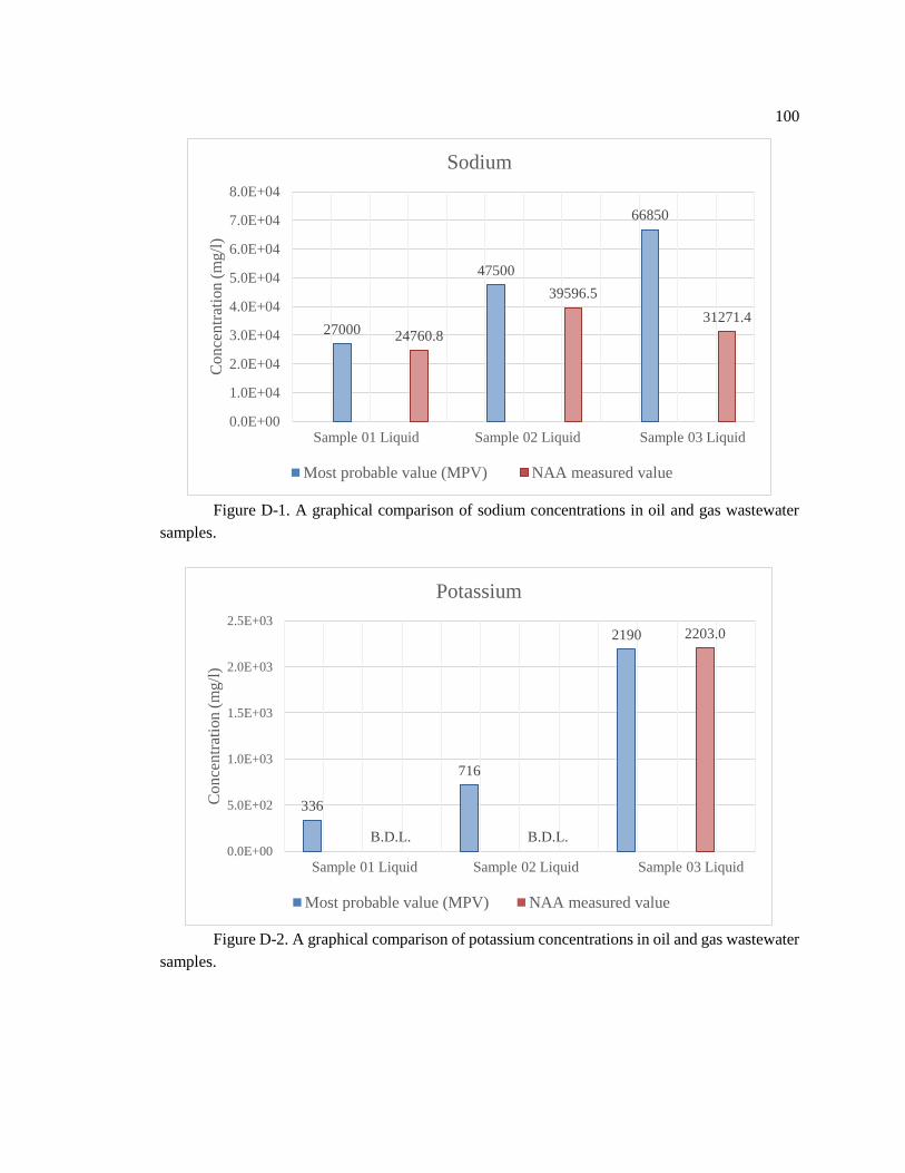
100
Figure D-1. A graphical comparison of sodium concentrations in oil and gas wastewater
samples.
Figure D-2. A graphical comparison of potassium concentrations in oil and gas wastewater
samples.
27000 24760.8
47500
39596.5
66850
31271.4
0.0E+00
1.0E+04
2.0E+04
3.0E+04
4.0E+04
5.0E+04
6.0E+04
7.0E+04
8.0E+04
Co
nce
ntr
atio
n (
mg/l
)
Sample 01 Liquid Sample 02 Liquid Sample 03 Liquid
Sodium
Most probable value (MPV) NAA measured value
336
B.D.L.
716
B.D.L.
2190 2203.0
0.0E+00
5.0E+02
1.0E+03
1.5E+03
2.0E+03
2.5E+03
Conce
ntr
atio
n (
mg/l
)
Sample 01 Liquid Sample 02 Liquid Sample 03 Liquid
Potassium
Most probable value (MPV) NAA measured value
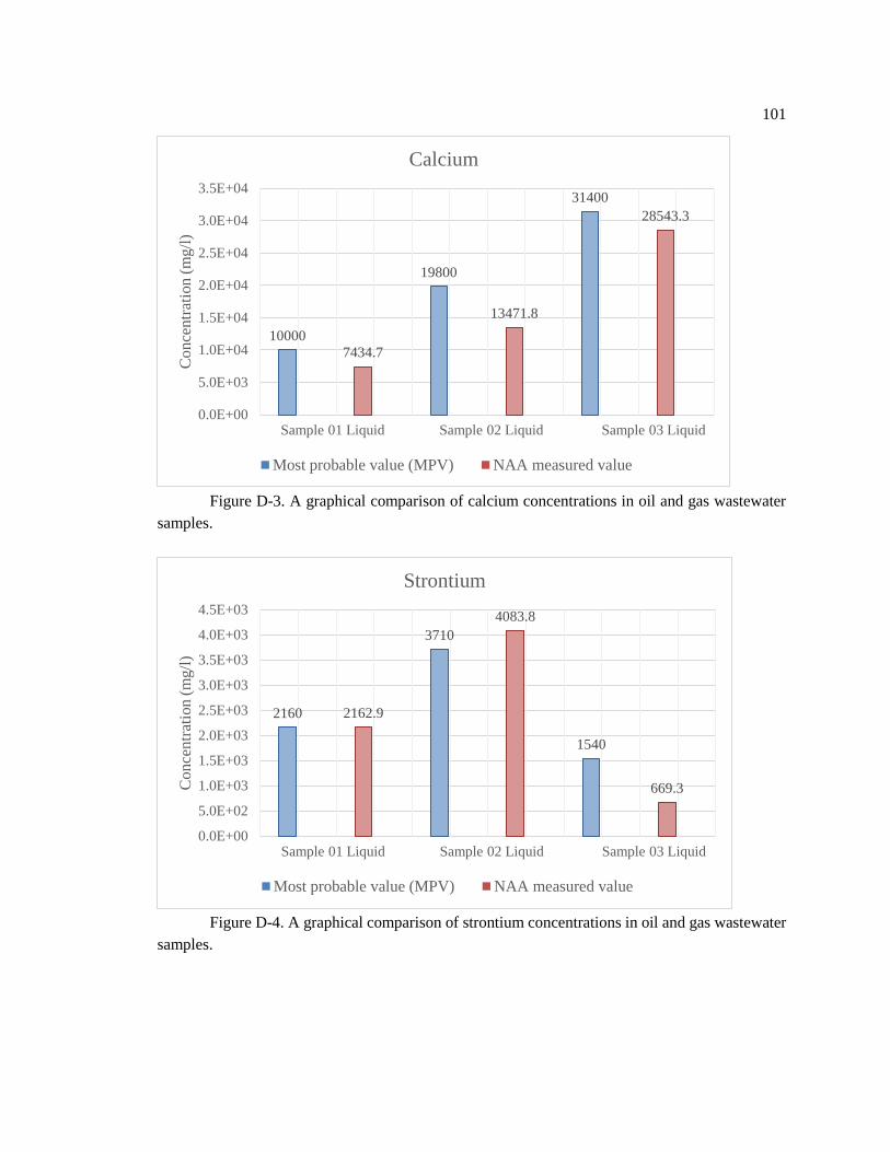
101
Figure D-3. A graphical comparison of calcium concentrations in oil and gas wastewater
samples.
Figure D-4. A graphical comparison of strontium concentrations in oil and gas wastewater
samples.
10000
7434.7
19800
13471.8
31400
28543.3
0.0E+00
5.0E+03
1.0E+04
1.5E+04
2.0E+04
2.5E+04
3.0E+04
3.5E+04C
on
cen
trat
ion
(m
g/l
)
Sample 01 Liquid Sample 02 Liquid Sample 03 Liquid
Calcium
Most probable value (MPV) NAA measured value
2160 2162.9
3710
4083.8
1540
669.3
0.0E+00
5.0E+02
1.0E+03
1.5E+03
2.0E+03
2.5E+03
3.0E+03
3.5E+03
4.0E+03
4.5E+03
Conce
ntr
atio
n (
mg/l
)
Sample 01 Liquid Sample 02 Liquid Sample 03 Liquid
Strontium
Most probable value (MPV) NAA measured value

102
Figure D-5. A graphical comparison of barium concentrations in oil and gas wastewater
samples.
Figure D-6. A graphical comparison of iron concentrations in oil and gas wastewater
samples.
659 622.4
13201221.8
6.12 7.20.0E+00
2.0E+02
4.0E+02
6.0E+02
8.0E+02
1.0E+03
1.2E+03
1.4E+03
1.6E+03
Co
nce
ntr
atio
n (
mg/l
)
Sample 01 Liquid Sample 02 Liquid Sample 03 Liquid
Barium
Most probable value (MPV) NAA measured value
64.854.3
94.982.8
169 165.1
0.0E+00
2.0E+01
4.0E+01
6.0E+01
8.0E+01
1.0E+02
1.2E+02
1.4E+02
1.6E+02
1.8E+02
2.0E+02
Co
nce
ntr
atio
n (
mg/l
)
Sample 01 Liquid Sample 02 Liquid Sample 03 Liquid
Iron
Most probable value (MPV) NAA measured value