characterization of electrical discharge machining plasmas · edm is used in a large number of...
TRANSCRIPT

POUR L'OBTENTION DU GRADE DE DOCTEUR ÈS SCIENCES
PAR
ingénieur physicien diplômé EPFde nationalité suisse et originaire de La Sagne (NE)
acceptée sur proposition du jury:
Lausanne, EPFL2006
Prof. R. Schaller, président du juryDr Ch. Hollenstein, directeur de thèse
Prof. M. Rappaz, rapporteurDr G. Wälder, rapporteurProf. J. Winter, rapporteur
characterization of electrical discharge machining plasmas
Antoine DESCOEUDRES
THÈSE NO 3542 (2006)
ÉCOLE POLYTECHNIQUE FÉDÉRALE DE LAUSANNE
PRÉSENTÉE LE 9 JUIN 2006
à LA FACULTÉ SCIENCES DE BASE
Centre de Recherche en Physique des Plasmas
SECTION DE PHYSIQUE

“La frousse, moi ! ... J’aime autant vousdire, mille tonnerres ! que quand je lerencontrerai, votre yéti, ça va faire desétincelles !”
le capitaine Haddock


Abstract
Electrical Discharge Machining (EDM) is a well-known machining technique since morethan fifty years. Its principle is to use the eroding effect on the electrodes of successiveelectric spark discharges created in a dielectric liquid. EDM is nowadays widely-usedin a large number of industrial areas. Nevertheless, few studies have been done on thedischarge itself and on the plasma created during this process. Further improvements ofEDM, especially for micro-machining, require a better control and understanding of thedischarge and of its interaction with the electrodes. In this work, the different phasesof the EDM process and the properties of the EDM plasma have been systematicallyinvestigated with electrical measurements, with imaging and with time- and spatially-resolved optical emission spectroscopy.
The pre-breakdown phase in water is characterized by the generation of numeroussmall hydrogen bubbles, created by electrolysis. Since streamers propagate more easily ina gaseous medium, these bubbles can facilitate the breakdown process. In oil, no bubblesare observed. Therefore, the breakdown mechanism in oil could be rather enhanced byparticles present in the electrode gap. Fast pulses of current and light are simultaneouslymeasured during the pre-breakdown. These pulses are characteristic of the propagation ofstreamers in the dielectric liquid. The pre-breakdown duration is not constant for givendischarge parameters, but distributed following a Weibull distribution. This shows thatthe breakdown is of stochastic nature.
After the breakdown, the plasma develops very rapidly (< 50 ns) and then remainsstable. The plasma light is particularly intense during the first 500 ns after the breakdownand weaker during the rest of the discharge, depending on the current intensity. While thegap distance is estimated to be around 10−100 µm, the discharge excites a broad volumearound the electrode gap, typically 200 µm in diameter. This volume grows slightly duringthe discharge. Vapor bubbles are generated in water and in oil by the heat released fromthe plasma. At the end of the discharge, the plasma implodes and disappears quickly.Light is still emitted after the discharge by incandescent metallic particles coming from theerosion of the workpiece. Their temperature is measured around 2’200 K, demonstratingthat they are still in a liquid state in the beginning of the post-discharge.
The spectroscopic analysis of the plasma light shows a strong Hα and continuumradiation, with many atomic metallic lines emitted by impurities coming from electrodeand workpiece materials. The EDM plasma is thus composed of species coming fromthe cracking of the dielectric molecules (mainly hydrogen in the case of water and oil),with contamination from the electrodes. The contamination is slightly higher in thevicinity of each electrode, and the contamination from the workpiece increases during the
i

ii ABSTRACT
discharge probably due to vaporization. The electron temperature, measured from copperline intensities with the two-line method, is found to be low. The temperature is around0.7 eV (∼ 8’100 K) in the whole plasma, slightly higher in the beginning of the discharge.The electron density has been measured from Stark broadening and shift measurementsof the Hα line. The density is extremely high, especially at the beginning of the discharge(> 2·1018 cm−3 during the first microsecond). Then it decreases with time, remainingnevertheless above 1016 cm−3 after 50 µs. During the whole discharge, the density isslightly higher in the plasma center. The EDM plasma has such a high density because itis formed from a liquid, and because it is constantly submitted to the pressure imposed bythe surrounding liquid. This extreme density produces spectra with strongly-broadenedspectral lines, especially the Hα line, and with an important continuum. During the firstmicrosecond when the density is at its maximum, spectral lines are so broadened thatthey are all merged into a continuum.
The low temperature and the high density of the EDM plasma make it weakly non-ideal. Its typical coupling parameter Γ is indeed around 0.3, reaching 0.45 during the firstmicrosecond. In this plasma, the Coulomb interactions between the charged particlesare thus of the same order as the mean thermal energy of the particles, which producescoupling phenomena. Spectroscopic results confirm the non-ideality of the EDM plasma.The strong broadening and shift of the Hα line and its asymmetric shape and complexstructure, the absence of the Hβ line, and the merging of spectral lines are typical of non-ideal plasmas. The EDM plasma has thus extreme physical properties, and the physicsinvolved is astonishingly complex.
Keywords: electrical discharge machining, EDM, plasma, spark, discharge, non-ideal plasma, optical emission spectroscopy, spectroscopy, imaging, breakdown, dielectric,liquid.
Version abrégée
L’électro-érosion (ou EDM pour Electrical Discharge Machining) est une technique d’usi-nage bien connue depuis plus de cinquante ans. Son principe est d’utiliser l’effet érosifsur les électrodes d’étincelles électriques successives créées dans un liquide diélectrique.L’électro-érosion est aujourd’hui très utilisée dans un grand nombre de secteurs industriels.Néanmoins, peu d’études ont été menées sur la décharge elle-même et sur le plasma créépendant ce processus. Les améliorations futures de l’électro-érosion, en particulier pourle micro-usinage, passent par un meilleur contrôle et une meilleure compréhension de ladécharge et de ses interactions avec les électrodes. Dans ce travail, les différentes phasesdu processus d’électro-érosion et les propriétés du plasma ont été étudiées de manièresystématique, à l’aide de mesures électriques, d’imagerie et de spectroscopie d’émissionoptique résolue en temps et en espace.
La phase de pré-décharge dans l’eau est caractérisée par la génération de nombreusespetites bulles d’hydrogène, créées par électrolyse. Puisque les streamers se propagent plusfacilement dans un milieu gazeux, ces bulles peuvent faciliter le processus de claquage.Dans l’huile, aucune bulle n’est observée. Ainsi, le mécanisme de claquage dans l’huilepourrait plutôt être facilité par des particules présentes dans l’espace inter-électrodes.Des impulsions rapides de courant et de lumière sont mesurées simultanément durant lapré-décharge. Ces impulsions sont caractéristiques de la propagation de streamers dans leliquide diélectrique. La durée de la pré-décharge n’est pas constante pour des paramètresde décharge donnés, mais elle est distribuée selon une distribution de Weibull. Ceci montreque le claquage est de nature stochastique.
Après le claquage, le plasma se développe très rapidement (< 50 ns) et reste ensuitestable. La lumière du plasma est particulièrement intense durant les premières 500 nssuivant le claquage et plus faible pendant le reste de la décharge, et dépend de l’intensité ducourant. Alors que l’espace inter-électrodes est estimé à environ 10−100 µm, la déchargeexcite un large volume autour des électrodes, d’un diamètre typique de 200 µm. Ce volumecroît légèrement pendant la décharge. Des bulles de vapeur sont générées aussi bien dansl’eau que dans l’huile, dû à la chaleur libérée par le plasma. A la fin de la décharge, leplasma implose et disparaît rapidement. De la lumière est encore émise après la déchargepar des particules métalliques incandescentes, provenant de l’érosion de la pièce. Leurtempérature a été mesurée à environ 2’200 K, ce qui démontre qu’elles sont toujours àl’état liquide au début de la post-décharge.
L’analyse spectroscopique de la lumière du plasma montre un forte radiation de laligne Hα et une forte émission continue, avec la présence de nombreuses lignes atomiquesmétalliques émises par des impuretés provenant des matériaux de l’électrode et de la
iii

iv VERSION ABREGEE
pièce. Ainsi, le plasma d’électro-érosion est composé d’espèces provenant de la dissociationdes molécules du diélectrique (principalement de l’hydrogène dans le cas de l’eau et del’huile), avec une contamination des électrodes. La contamination est légèrement plusforte au voisinage de chaque électrode, et la contamination venant de la pièce augmenteau cours de la décharge, probablement à cause de son évaporation. La température élec-tronique, mesurée à partir des intensités de lignes de cuivre avec la méthode dite two-linemethod, est basse. La température est autour de 0.7 eV (∼ 8’100 K) dans tout le plasma,légèrement plus haute au début de la décharge. La densité électronique a été mesurée àpartir de l’élargissement et du déplacement par effet Stark de la ligne Hα. La densité estextrêmement élevée, particulièrement au début de la décharge (> 2·1018 cm−3 durant lapremière microseconde). Elle décroît ensuite avec le temps, restant néanmoins toujoursau-dessus de 1016 cm−3 après 50 µs. Pendant toute la décharge, la densité est légèrementplus élevée au centre du plasma. Le plasma d’électro-érosion a une densité si élevée caril est formé à partir d’un liquide, et parce qu’il est constamment soumis à la pressionimposée par le liquide environnant. Cette densité extrême produit des spectres avecdes lignes spectrales très élargies, particulièrement la ligne Hα, et avec une importanteradiation continue. Pendant la première microseconde où la densité est à son maximum,les lignes spectrales sont tellement élargies qu’elles fusionnent et ne forment qu’un continu.
La basse température et la haute densité du plasma d’électro-érosion le rendent faible-ment non-idéal. Son paramètre de couplage Γ typique est en effet autour de 0.3, atteignant0.45 pendant la première microseconde. Dans ce plasma, les interactions coulombiennesentre les particules chargées sont ainsi du même ordre que l’énergie thermique moyennedes particules, ce qui produit des phénomènes de couplage. Des résultats de spectroscopieconfirment la non-idéalité du plasma d’électro-érosion. Le fort élargissement et déplace-ment de la ligne Hα ainsi que sa forme asymétrique et sa structure complexe, l’absencede la ligne Hβ, et la fusion des lignes spectrales sont en effet typiques des plasmas non-idéaux. Le plasma d’électro-érosion possède ainsi des propriétés physiques extrêmes, etla physique y relative est étonnamment complexe.
Mots-clés: électro-érosion, EDM, plasma, étincelle, décharge, plasma non-idéal, spec-troscopie d’émission optique, spectroscopie, imagerie, claquage, diélectrique, liquide.
Contents
Abstract i
Version abrégée iii
1 Introduction 11.1 Electrical Discharge Machining (EDM) . . . . . . . . . . . . . . . . . . . . 1
1.1.1 Principles . . . . . . . . . . . . . . . . . . . . . . . . . . . . . . . . 21.1.2 History . . . . . . . . . . . . . . . . . . . . . . . . . . . . . . . . . . 41.1.3 State of the art . . . . . . . . . . . . . . . . . . . . . . . . . . . . . 8
1.2 Purpose and structure of the work . . . . . . . . . . . . . . . . . . . . . . . 8
2 EDM plasmas : Background 112.1 Discharges in gases . . . . . . . . . . . . . . . . . . . . . . . . . . . . . . . 11
2.1.1 Spark, arc, glow & co. . . . . . . . . . . . . . . . . . . . . . . . . . 112.1.2 Sparks and streamers . . . . . . . . . . . . . . . . . . . . . . . . . . 122.1.3 Electric arcs and cathode spots . . . . . . . . . . . . . . . . . . . . 14
2.2 Discharges in dielectric liquids . . . . . . . . . . . . . . . . . . . . . . . . . 182.3 Other similar plasmas . . . . . . . . . . . . . . . . . . . . . . . . . . . . . 22
3 Experimental setup and diagnostics 253.1 Electrical discharge machining device . . . . . . . . . . . . . . . . . . . . . 253.2 Electrical measurements . . . . . . . . . . . . . . . . . . . . . . . . . . . . 27
3.2.1 Discharge measurements . . . . . . . . . . . . . . . . . . . . . . . . 273.2.2 Pre-breakdown measurements . . . . . . . . . . . . . . . . . . . . . 28
3.3 Plasma light intensity measurements . . . . . . . . . . . . . . . . . . . . . 293.4 Imaging . . . . . . . . . . . . . . . . . . . . . . . . . . . . . . . . . . . . . 303.5 Optical emission spectroscopy . . . . . . . . . . . . . . . . . . . . . . . . . 32
3.5.1 Principles . . . . . . . . . . . . . . . . . . . . . . . . . . . . . . . . 323.5.2 Electron temperature measurement . . . . . . . . . . . . . . . . . . 333.5.3 Electron density measurement . . . . . . . . . . . . . . . . . . . . . 353.5.4 General experimental setup . . . . . . . . . . . . . . . . . . . . . . 373.5.5 Experimental setup for time-resolved spectroscopy . . . . . . . . . . 403.5.6 Experimental setup for spatially-resolved spectroscopy . . . . . . . 40
3.6 Experimental difficulties . . . . . . . . . . . . . . . . . . . . . . . . . . . . 41
v

vi CONTENTS
4 Pre-breakdown of EDM discharges 454.1 Bubbles . . . . . . . . . . . . . . . . . . . . . . . . . . . . . . . . . . . . . 454.2 Pre-breakdown current . . . . . . . . . . . . . . . . . . . . . . . . . . . . . 464.3 Pre-breakdown duration . . . . . . . . . . . . . . . . . . . . . . . . . . . . 50
5 Imaging diagnostics of EDM discharges 535.1 Imaging of the EDM process . . . . . . . . . . . . . . . . . . . . . . . . . . 53
5.1.1 Erosion . . . . . . . . . . . . . . . . . . . . . . . . . . . . . . . . . 535.1.2 Bubbles . . . . . . . . . . . . . . . . . . . . . . . . . . . . . . . . . 545.1.3 Short-circuit . . . . . . . . . . . . . . . . . . . . . . . . . . . . . . . 555.1.4 Reproducibility . . . . . . . . . . . . . . . . . . . . . . . . . . . . . 56
5.2 Plasma imaging . . . . . . . . . . . . . . . . . . . . . . . . . . . . . . . . . 565.2.1 Evolution of the plasma light intensity . . . . . . . . . . . . . . . . 565.2.2 Typical plasma image . . . . . . . . . . . . . . . . . . . . . . . . . 585.2.3 Plasma evolution . . . . . . . . . . . . . . . . . . . . . . . . . . . . 595.2.4 Effect of the discharge current . . . . . . . . . . . . . . . . . . . . . 595.2.5 Hα emission . . . . . . . . . . . . . . . . . . . . . . . . . . . . . . . 60
5.3 Beginning of the discharge : Fast imaging . . . . . . . . . . . . . . . . . . 615.4 End of the discharge and post-discharge . . . . . . . . . . . . . . . . . . . 62
6 Optical emission spectroscopy of EDM plasmas 676.1 Time-integrated emission spectra . . . . . . . . . . . . . . . . . . . . . . . 67
6.1.1 Typical spectrum . . . . . . . . . . . . . . . . . . . . . . . . . . . . 676.1.2 Effect of the dielectric . . . . . . . . . . . . . . . . . . . . . . . . . 696.1.3 Effect of the electrode material . . . . . . . . . . . . . . . . . . . . 706.1.4 Effect of the electrode polarity . . . . . . . . . . . . . . . . . . . . . 726.1.5 Effect of the discharge current . . . . . . . . . . . . . . . . . . . . . 736.1.6 Effect of the discharge on-time . . . . . . . . . . . . . . . . . . . . . 746.1.7 First estimation of electron density and temperature . . . . . . . . 75
6.2 Time-resolved emission spectra . . . . . . . . . . . . . . . . . . . . . . . . 766.2.1 Merging of atomic lines . . . . . . . . . . . . . . . . . . . . . . . . . 766.2.2 Evolution of the electron temperature . . . . . . . . . . . . . . . . . 766.2.3 Evolution of the electron density . . . . . . . . . . . . . . . . . . . 77
6.3 Spatially-resolved emission spectra . . . . . . . . . . . . . . . . . . . . . . 796.3.1 Asymmetry of the contamination . . . . . . . . . . . . . . . . . . . 796.3.2 Electron temperature profile . . . . . . . . . . . . . . . . . . . . . . 806.3.3 Electron density profile . . . . . . . . . . . . . . . . . . . . . . . . . 81
6.4 Time- and spatially-resolved emission spectra . . . . . . . . . . . . . . . . 826.4.1 Evolution of the contamination . . . . . . . . . . . . . . . . . . . . 826.4.2 Evolution of the electron temperature profiles . . . . . . . . . . . . 836.4.3 Evolution of the electron density profiles . . . . . . . . . . . . . . . 84
CONTENTS vii
7 Non-ideality of EDM plasmas 877.1 Plasma coupling parameter Γ . . . . . . . . . . . . . . . . . . . . . . . . . 877.2 Spectroscopic signs of the non-ideality . . . . . . . . . . . . . . . . . . . . 90
7.2.1 Broadening and shift of Hα . . . . . . . . . . . . . . . . . . . . . . . 907.2.2 Asymmetry and structure of Hα . . . . . . . . . . . . . . . . . . . . 907.2.3 Absence of Hβ and line merging . . . . . . . . . . . . . . . . . . . . 937.2.4 Inglis-Teller relation . . . . . . . . . . . . . . . . . . . . . . . . . . 94
7.3 Summary of the physical properties of EDM plasmas . . . . . . . . . . . . 95
8 Conclusions 101
A Stark broadening and shift of hydrogen spectral lines 105A.1 The Stark effect on hydrogen levels . . . . . . . . . . . . . . . . . . . . . . 105A.2 Consequences of the Stark effect on Hα emission . . . . . . . . . . . . . . . 107
References 111
Acknowledgments 123
Curriculum Vitae 125

viii CONTENTS
Chapter 1
Introduction
1.1 Electrical Discharge Machining (EDM)
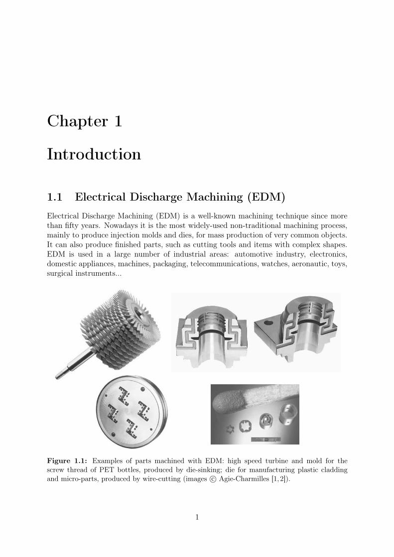
Electrical Discharge Machining (EDM) is a well-known machining technique since morethan fifty years. Nowadays it is the most widely-used non-traditional machining process,mainly to produce injection molds and dies, for mass production of very common objects.It can also produce finished parts, such as cutting tools and items with complex shapes.EDM is used in a large number of industrial areas: automotive industry, electronics,domestic appliances, machines, packaging, telecommunications, watches, aeronautic, toys,surgical instruments...
Figure 1.1: Examples of parts machined with EDM: high speed turbine and mold for thescrew thread of PET bottles, produced by die-sinking; die for manufacturing plastic claddingand micro-parts, produced by wire-cutting (images c© Agie-Charmilles [1, 2]).
1
2 CHAPTER 1. INTRODUCTION
The advantages of EDM over traditional methods such as milling or grinding are mul-tiple. Any material that conducts electricity can be machined, whatever its hardness(hardened steel, tungsten carbide, special alloys for aerospace applications, for example).Furthermore, complex cutting geometry, sharp angles and internal corners can be pro-duced. Final surface state with low rugosity (< 100 nm) and precise machining (∼ 1 µm)are other important advantages. Moreover, there is no mechanical stress on the machinedpiece, no rotation of workpiece or tool is necessary, and the machines have a high au-tonomy. On the other hand, the disadvantages are the relatively low material removalrate (order of 100 mm3/minute), surface modification of the machined workpiece (“whitelayer” and heat affected zone, typical depth ∼ 50 µm), and limited size of workpiece andtool, for example.
1.1.1 Principles
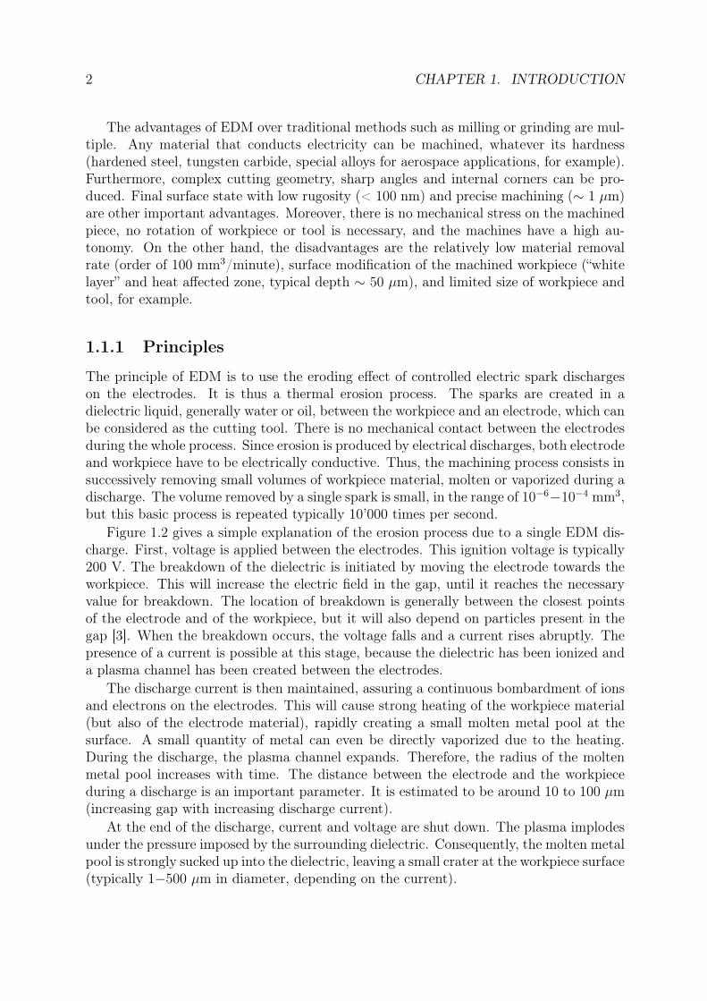
The principle of EDM is to use the eroding effect of controlled electric spark dischargeson the electrodes. It is thus a thermal erosion process. The sparks are created in adielectric liquid, generally water or oil, between the workpiece and an electrode, which canbe considered as the cutting tool. There is no mechanical contact between the electrodesduring the whole process. Since erosion is produced by electrical discharges, both electrodeand workpiece have to be electrically conductive. Thus, the machining process consists insuccessively removing small volumes of workpiece material, molten or vaporized during adischarge. The volume removed by a single spark is small, in the range of 10−6−10−4 mm3,but this basic process is repeated typically 10’000 times per second.
Figure 1.2 gives a simple explanation of the erosion process due to a single EDM dis-charge. First, voltage is applied between the electrodes. This ignition voltage is typically200 V. The breakdown of the dielectric is initiated by moving the electrode towards theworkpiece. This will increase the electric field in the gap, until it reaches the necessaryvalue for breakdown. The location of breakdown is generally between the closest pointsof the electrode and of the workpiece, but it will also depend on particles present in thegap [3]. When the breakdown occurs, the voltage falls and a current rises abruptly. Thepresence of a current is possible at this stage, because the dielectric has been ionized anda plasma channel has been created between the electrodes.
The discharge current is then maintained, assuring a continuous bombardment of ionsand electrons on the electrodes. This will cause strong heating of the workpiece material(but also of the electrode material), rapidly creating a small molten metal pool at thesurface. A small quantity of metal can even be directly vaporized due to the heating.During the discharge, the plasma channel expands. Therefore, the radius of the moltenmetal pool increases with time. The distance between the electrode and the workpieceduring a discharge is an important parameter. It is estimated to be around 10 to 100 µm(increasing gap with increasing discharge current).
At the end of the discharge, current and voltage are shut down. The plasma implodesunder the pressure imposed by the surrounding dielectric. Consequently, the molten metalpool is strongly sucked up into the dielectric, leaving a small crater at the workpiece surface(typically 1−500 µm in diameter, depending on the current).

1.1. ELECTRICAL DISCHARGE MACHINING (EDM) 3voltage
curr
ent
time
time
(a) (b) (c) (d) (e)
(a) Pre-breakdown :voltage applied
between the electrodeand the workpiece
(b) Breakdown :dielectric breakdown,
creation of theplasma channel
(c) Discharge :heating, melting and
vaporizing of theworkpiece material
(d) End of the discharge :plasma implosion,removing of the
molten metal pool
(e) Post-discharge :solidifying and flushingof the eroded particles
by the dielectric
Figure 1.2: Principle of the EDM process.
The liquid dielectric plays a crucial role during the whole process: it cools down theelectrodes, it guarantees a high plasma pressure and therefore a high removing force onthe molten metal when the plasma collapses, it solidifies the molten metal into smallspherical particles, and it also flushes away these particles. The post-discharge is in facta crucial stage, during which the electrode gap is cleaned of the removed particles for thenext discharge. If particles stay in the gap, the electrical conductivity of the dielectricliquid increases, leading to a bad control of the process and poor machining quality. Toenhance the flushing of particles, the dielectric is generally flowing through the gap. Inaddition, the electrode movement can be pulsed, typically every second, performing alarge retreat movement. This pulsing movement also enhances the cleaning, on a largerscale, by bringing “fresh” dielectric into the gap.
The material removal rate can be asymmetrically distributed between the electrode(wear) and the workpiece (erosion). The asymmetry is mostly due to the different ma-terials of the electrodes. But it also depends on the electrode polarity, on the durationof the discharges and on the discharge current. Note that by convention, the polarity iscalled positive when the electrode is polarized positively towards the workpiece, negativeotherwise. By carefully choosing the discharge parameters, 0.1% wear and 99.9% erosioncan be achieved.
4 CHAPTER 1. INTRODUCTION
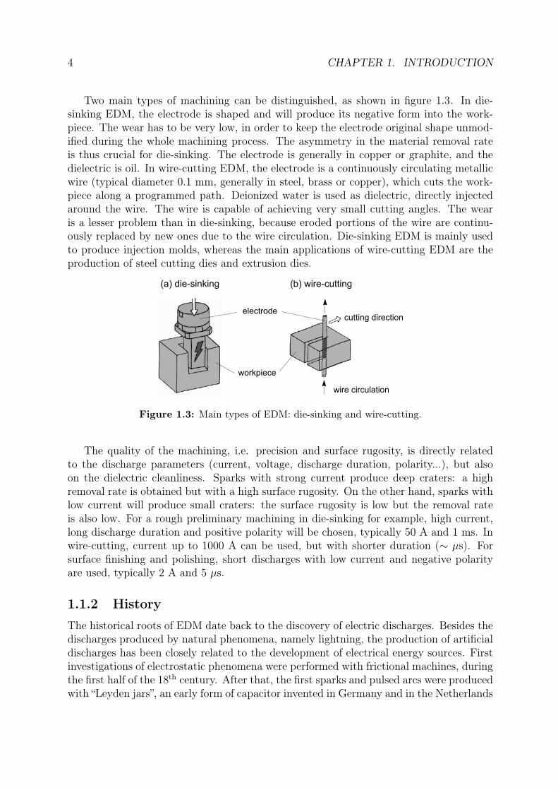
Two main types of machining can be distinguished, as shown in figure 1.3. In die-sinking EDM, the electrode is shaped and will produce its negative form into the work-piece. The wear has to be very low, in order to keep the electrode original shape unmod-ified during the whole machining process. The asymmetry in the material removal rateis thus crucial for die-sinking. The electrode is generally in copper or graphite, and thedielectric is oil. In wire-cutting EDM, the electrode is a continuously circulating metallicwire (typical diameter 0.1 mm, generally in steel, brass or copper), which cuts the work-piece along a programmed path. Deionized water is used as dielectric, directly injectedaround the wire. The wire is capable of achieving very small cutting angles. The wearis a lesser problem than in die-sinking, because eroded portions of the wire are continu-ously replaced by new ones due to the wire circulation. Die-sinking EDM is mainly usedto produce injection molds, whereas the main applications of wire-cutting EDM are theproduction of steel cutting dies and extrusion dies.
(a) die-sinking (b) wire-cutting
electrode
workpiece
cutting direction
wire circulation
Figure 1.3: Main types of EDM: die-sinking and wire-cutting.
The quality of the machining, i.e. precision and surface rugosity, is directly relatedto the discharge parameters (current, voltage, discharge duration, polarity...), but alsoon the dielectric cleanliness. Sparks with strong current produce deep craters: a highremoval rate is obtained but with a high surface rugosity. On the other hand, sparks withlow current will produce small craters: the surface rugosity is low but the removal rateis also low. For a rough preliminary machining in die-sinking for example, high current,long discharge duration and positive polarity will be chosen, typically 50 A and 1 ms. Inwire-cutting, current up to 1000 A can be used, but with shorter duration (∼ µs). Forsurface finishing and polishing, short discharges with low current and negative polarityare used, typically 2 A and 5 µs.
1.1.2 History
The historical roots of EDM date back to the discovery of electric discharges. Besides thedischarges produced by natural phenomena, namely lightning, the production of artificialdischarges has been closely related to the development of electrical energy sources. Firstinvestigations of electrostatic phenomena were performed with frictional machines, duringthe first half of the 18th century. After that, the first sparks and pulsed arcs were producedwith “Leyden jars”, an early form of capacitor invented in Germany and in the Netherlands
1.1. ELECTRICAL DISCHARGE MACHINING (EDM) 5
around 1745 [4] (see figure 1.4 (a)). More powerful discharges were created by puttingseveral Leyden jars in parallel, creating thus a “battery”. Although scientists of this periodsensed that the nature of these artificial discharges was the same as the nature of lightning,the understanding of the observed phenomena was very incomplete.
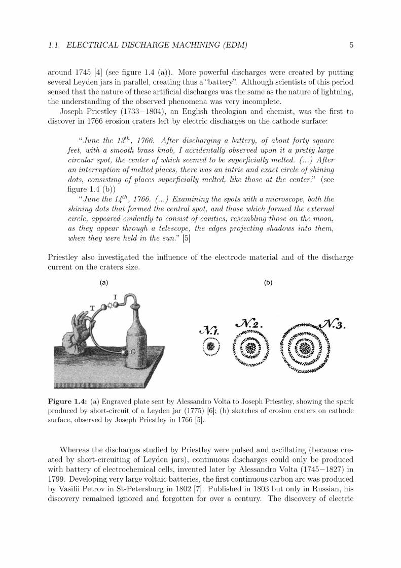
Joseph Priestley (1733−1804), an English theologian and chemist, was the first todiscover in 1766 erosion craters left by electric discharges on the cathode surface:
“June the 13th, 1766. After discharging a battery, of about forty squarefeet, with a smooth brass knob, I accidentally observed upon it a pretty largecircular spot, the center of which seemed to be superficially melted. (...) Afteran interruption of melted places, there was an intrie and exact circle of shiningdots, consisting of places superficially melted, like those at the center.” (seefigure 1.4 (b))
“June the 14th, 1766. (...) Examining the spots with a microscope, both theshining dots that formed the central spot, and those which formed the externalcircle, appeared evidently to consist of cavities, resembling those on the moon,as they appear through a telescope, the edges projecting shadows into them,when they were held in the sun.” [5]
Priestley also investigated the influence of the electrode material and of the dischargecurrent on the craters size.
Figure 1.4: (a) Engraved plate sent by Alessandro Volta to Joseph Priestley, showing the sparkproduced by short-circuit of a Leyden jar (1775) [6]; (b) sketches of erosion craters on cathodesurface, observed by Joseph Priestley in 1766 [5].
Whereas the discharges studied by Priestley were pulsed and oscillating (because cre-ated by short-circuiting of Leyden jars), continuous discharges could only be producedwith battery of electrochemical cells, invented later by Alessandro Volta (1745−1827) in1799. Developing very large voltaic batteries, the first continuous carbon arc was producedby Vasilii Petrov in St-Petersburg in 1802 [7]. Published in 1803 but only in Russian, hisdiscovery remained ignored and forgotten for over a century. The discovery of electric

6 CHAPTER 1. INTRODUCTION
arcs is thus often attributed to Humphry Davy (1778−1829). Unaware of Petrov’s work,he re-discovered independently carbon arcs around 1808, using the huge voltaic battery ofthe Royal Institution of London (see figure 1.5 (a)). By separating two horizontal carbonelectrodes connected to the battery, Davy created a bright and stable discharge. Theshape of this discharge was arched, giving its name to the phenomenon.
Development of devices using electric arcs for lighting purposes followed quickly. Swissnatural philosopher Auguste-Arthur de la Rive (1801−1873) proved in 1820 that arcs canalso burn in vacuum, by creating a discharge in an exhausted glass vessel. Figure 1.5 (b)shows examples of these early carbon arc lamps.
Figure 1.5: (a) Public demonstration of the carbon arc discharge, probably by Humphry Davyin the Royal Institution of London (early 19th century) [7]. The picture below shows the basementfilled with a huge battery, used to create the discharge; (b) early carbon arc lamps in air (left)and in exhausted glass vessel (right), also known as “Davy’s electric eggs” or “de la Rive’s electriceggs” [7].
With sophistication of electric sources and industrialization, Auguste de Meritens(1834−1898) developed in 1881 in France a second major application using electric arcs.He used the heat produced by an arc for joining lead plates, inventing the principle of arcwelding. Nowadays, electric arcs are also used for coating deposition, metal processing,plasma spraying and as high power switches, for example [8].
The history of EDM itself begins in 1943, with the invention of its principle by Russianscientists Boris and Natalya Lazarenko in Moscow. The Soviet government assigned themto investigate the wear caused by sparking between tungsten electrical contacts, a problemwhich was particularly critical for maintenance of automotive engines during the secondworld war. Putting the electrodes in oil, they found that the sparks were more uniformand predictable than in air. They had then the idea to reverse the phenomenon, andto use controlled sparking as an erosion method [9]. Though they could not solve theoriginal wear problem, the Lazarenkos developed during the war the first EDM machines,

1.1. ELECTRICAL DISCHARGE MACHINING (EDM) 7
which were very useful to erode hard metals such as tungsten or tungsten carbide. The“Lazarenko circuit” remained the standard EDM generator for years.
In the 1950’s, progress was made on understanding the erosion phenomenon [10–12].It is also during this period that industries produced the first EDM machines. Swissindustries were involved very early in this market, and still remain leaders nowadays.Agie was founded in 1954, and les Ateliers des Charmilles produced their first machine in1955. Due to the poor quality of electronic components, the performances of the machineswere limited at this time.
2005
1955
Figure 1.6: 50 years of evolution in EDM machines: Eleroda D1 (1955) andRobofil 2050 TW (2005) from Charmilles (images c© Charmilles Technologies [1]).
In the 1960’s, the development of the semi-conductor industry permitted considerableimprovements in EDM machines. Die-sinking machines became reliable and producedsurfaces with controlled quality, whereas wire-cutting machines were still at their verybeginning.
With the introduction of numerical position control in the late 1960’s and early 1970’s,the movements of electrodes became much more precise. This major improvement pushedforward the performance of wire-cutting machines. Computer numerical controlled sys-tems (CNC) improved further the performance of EDM in the mid 1970’s.
During the following decades, efforts were principally made in generator design, processautomatization, servo-control and robotics. Applications in micro-machining became alsoof interest during the 1980’s [13]. It is also from this period that the world market ofEDM began to increase strongly, and that specific applied EDM research took over basicEDM research [14]. Finally, new methods for EDM process control arose in the 1990’s:fuzzy control and neural networks.
8 CHAPTER 1. INTRODUCTION
1.1.3 State of the art
Fifty years after the first industrial machine, EDM has made considerable progress. Recentimprovements in machining speed, accuracy and roughness have been achieved mostlywith improvements in robotics, automatization, process control, dielectric, flushing andgenerator design [15–18]. The other main research domains are the machining of non-conductive materials such as ceramics [19, 20], micro-machining [21–24], characterizationand improvement in the machined surface quality [25, 26], and modelling of the EDMprocess [27–29]. But so far, few studies have been done on the discharge itself, which liesat the heart of the process.
However, in various fields, breakdown in dielectric liquids or solids have already beenstudied: pre-breakdown and breakdown in different liquids [30, 31] and condensed mat-ter [32], exploding wires in water [33], laser produced plasma in transformer oil [34], andTeflon capillary discharges [35] for example. These plasmas have similar properties tothose of the EDM plasma.
Though EDM keeps unmatched abilities such as the machining of hard materials andcomplex geometries, this technique has to evolve constantly in order to stay competitiveand economically interesting in the modern tooling market against other traditional ornew machining techniques [17,18,36].
1.2 Purpose and structure of the work
Further improvements in EDM performances, especially for micro-machining, require abetter control and understanding of the discharge, and of its interaction with the elec-trodes. A better comprehension of the sparking process will also reduce problems relatedto its stochastic nature.
Until now, process optimization relied almost only on empirical methods and recipes.It is necessary to go beyond this empirical optimization, and to use reliable numericalmodels to predict important parameters, such as the material removal rate and wear forexample.
Although EDM is quite old, only a few theoretical and numerical studies on the EDMplasma exist [37–40], mainly due to the complex physics involved in this process. TheEDM process mixes indeed breakdown of liquids, plasma physics, heat transfer, radi-ation, hydrodynamics, materials science, electrodynamics... These models still containseveral parameters which are empirically determined or artificially introduced. Further-more, experimental characterization of the EDM plasma is lacking. Some spectroscopicmeasurements have already been made but remain very incomplete [41, 42]. As we willsee later (section 3.6), the EDM plasma is experimentally difficult to investigate. Thesedifficulties are the main cause for the lack of experimental data, which are neverthelessessential as inputs and for the validation of numerical models.
The purpose of this work is thus a systematic experimental investigation of the EDMplasma, in order to measure its physical properties and to improve the understandingof its complex basic physics. Besides the industrial aspect, the study of this plasma is

1.2. PURPOSE AND STRUCTURE OF THE WORK 9
also of fundamental interest. Other works on similar plasmas, notably measurements oftheir density and temperature (see sections 2.2 and 2.3), showed that they can be classedamong non-ideal or strongly coupled plasmas. Such plasmas have very interesting physicalproperties and are still not well known [43–46]. Strongly coupled plasmas produced inthe lab are interesting also for astrophysical studies, because deep layers of giant planetsand superdense plasmas of the matter of white dwarves are of this kind [43].
This work is one part of a special EDM research project, initiated by the innovationcommittee of the Technology-Oriented Program NANO 21 (project n 5768.2). Thisproject was a collaboration involving:
• Charmilles Technologies, as the industrial partner (Dr G. Wälder);
• the Centre de Recherches en Physique des Plasmas (CRPP) of the Ecole Polytech-nique Fédérale de Lausanne (EPFL), for the study of the plasma (Dr Ch. Hollen-stein);
• the Laboratoire de Simulation des Matériaux (LSMX) of the EPFL, for a numericalmodel of the temperature evolution in the workpiece surface (Prof. M. Rappaz);
• the Département de Physique de la Matière Condensée (DPMC) of the Université deGenève, for the study of metallurgical processes occurring at the workpiece surface(Prof. R. Flükiger);
• the Electrochemistry group of the Bern Universität, for the study of corrosion as-pects of the EDM process (Prof. H. Siegenthaler).
The present manuscript is structured as follows: we will first present in chapter 2 ageneral background for the understanding of EDM plasmas, i.e. a brief summary of exist-ing knowledge about similar phenomena and plasmas. The different experimental setupsand plasma diagnostics used in this work are described in chapter 3, and the experimentalresults are presented and discussed in chapters 4 (results about pre-breakdown), 5 (imag-ing results) and 6 (spectroscopy results). Chapter 7 treats the non-ideal character of EDMplasmas, and also gives a summary of their measured physical properties. Finally, generalconclusions are given in chapter 8.

10 CHAPTER 1. INTRODUCTION

Chapter 2
EDM plasmas : Background
Although EDM discharges take place in a dielectric liquid, the first section of this chapterwill deal with discharges in gases. They have been extensively studied [47–49], and havecommon features with discharges in liquids. After that, a brief review about the specificcharacteristics of discharges in liquids will be given in the second section. Finally, otherplasmas similar to the EDM plasmas are presented in the last section.
2.1 Discharges in gases
2.1.1 Spark, arc, glow & co.
Depending on the gas pressure, the electrode gap and the electrode configuration, severaldischarge regimes can be distinguished. They can be classified according to their current-voltage characteristics, as shown in figure 2.1.
voltage
current
Townsenddischarge
coronaspark
arc
normalglow
abnormalglow
low-pressure
atmospheric pressure
Figure 2.1: Schematic current-voltage characteristics of the different types of discharges ingases [47,48].
11
12 CHAPTER 2. EDM PLASMAS : BACKGROUND
Four main types of steady or quasi-steady processes exist:
• the Townsend’s dark discharge, characterized by a very weak current (∼ 10−8 A);
• the glow discharge, widely used in many industrial processes, operating at lowcurrent (∼ 10−2 A), fairly high voltage (∼ 1 kV) and low pressure (∼ mbar). Theglow plasma is weakly ionized and in a non-equilibrium state, and is visible as auniform glowing column. As in the Townsend’s discharge, electrons are emitted byion impacts on the cold cathode;
• the corona discharge, also at low current (∼ 10−6 A) but at atmospheric pressure.Corona discharges develop locally (typically around sharp ends of wires) in stronglynon-uniform electric field;
• the arc discharge, characterized by high current (∼ 100 A), low voltage (∼ 10 V)and a bright light emission. The arc discharge differs from the glow dischargein the electron emission mechanism. In arcs, electrons are emitted by thermionicprocesses, due to the heating of the cathode. The plasma of high pressure arcs canbe considered to be in a state of thermodynamic equilibrium.
On the contrary to Townsend, glow, corona and arc discharges, the spark dischargeis not a steady process but a transient process, i.e. an unstable transition state of limitedlifetime towards a more stable regime (see figure 2.1). To be perfectly rigorous, it wouldbe more proper to say “spark breakdown” than “spark discharge”, since it is a transitionmechanism and not a state resulting from a transition [48]. However, we will keep (abu-sively but for clarity) the term spark discharge or simply discharge when speaking aboutthe period during which the EDM plasma exists (part c in figure 1.2), and the term break-down will refer to the transition from the no-plasma situation to the plasma situation(part b in figure 1.2).
2.1.2 Sparks and streamers
Since the plasma created during the EDM process is precisely a spark, it is worthwhileto describe this type of discharge in more detail. Note that lightning shows beautifulexamples of giant spark discharges.
The breakdown phenomenon leading to the creation of a spark is complex. The break-down is too fast to be explained by repetitive electron avalanches through secondary cath-ode emission, as in low pressure discharges. It consists rather of a very rapid growth of athin weakly-ionized channel called a streamer, from one electrode to the other.
A streamer is formed from an intensive primary electron avalanche, starting from thecathode (see figure 2.2 (a)). A space charge field is associated with this avalanche, dueto the polarization of charges inside it. This electric field increases with the avalanchepropagation and growth. The avalanche has to reach a certain amplification before itcan create a streamer. As soon as the space charge field is comparable or exceeding theapplied external field, a weakly ionized region can be created due to this amplification ofthe electric field: the streamer is thus initiated.
2.1. DISCHARGES IN GASES 13
(a) electron avalanche (b) positive streamer (c) negative streamer
anode +
cathode -
anode +
cathode -
anode +
cathode -
+
++
+++
++
++
str
eam
er
secondaryavalanches
+ ++
+
+ ++ +++ +
+
_ __ ____
__
_
___
_
_
_ _
_
+
++
+
+ _
+
+_ +
_ _
+
_ __ _ ___
_
_
_
_
_
++
++
+hn
pro
pagation
t > t2 1t1+
+ +___
t > t2 1t1
t > t2 1t1
++ +
_ __+ ++ +
++_
__ +
__
__
+++_
_
+_ _+
++
__
space chargefield
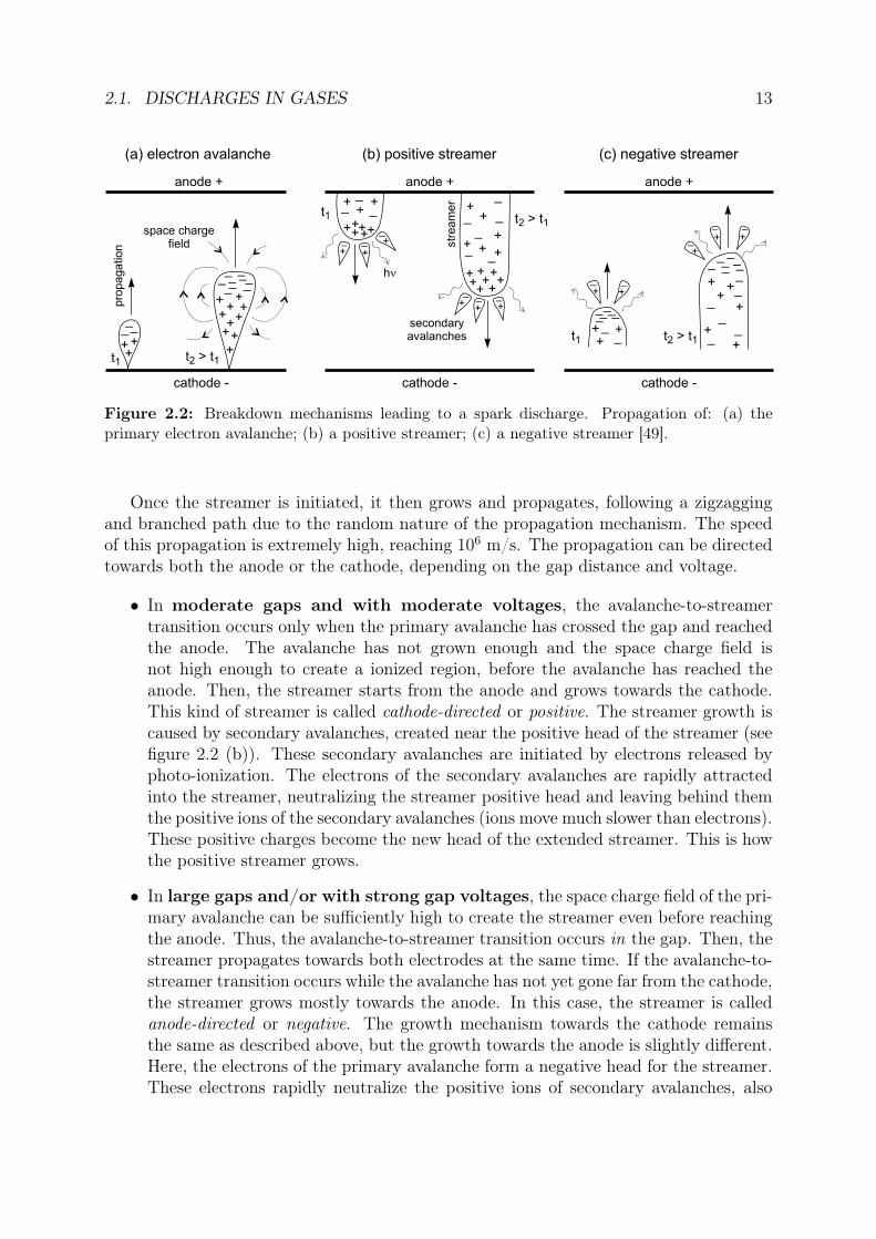
Figure 2.2: Breakdown mechanisms leading to a spark discharge. Propagation of: (a) theprimary electron avalanche; (b) a positive streamer; (c) a negative streamer [49].
Once the streamer is initiated, it then grows and propagates, following a zigzaggingand branched path due to the random nature of the propagation mechanism. The speedof this propagation is extremely high, reaching 106 m/s. The propagation can be directedtowards both the anode or the cathode, depending on the gap distance and voltage.
• In moderate gaps and with moderate voltages, the avalanche-to-streamertransition occurs only when the primary avalanche has crossed the gap and reachedthe anode. The avalanche has not grown enough and the space charge field isnot high enough to create a ionized region, before the avalanche has reached theanode. Then, the streamer starts from the anode and grows towards the cathode.This kind of streamer is called cathode-directed or positive. The streamer growth iscaused by secondary avalanches, created near the positive head of the streamer (seefigure 2.2 (b)). These secondary avalanches are initiated by electrons released byphoto-ionization. The electrons of the secondary avalanches are rapidly attractedinto the streamer, neutralizing the streamer positive head and leaving behind themthe positive ions of the secondary avalanches (ions move much slower than electrons).These positive charges become the new head of the extended streamer. This is howthe positive streamer grows.
• In large gaps and/or with strong gap voltages, the space charge field of the pri-mary avalanche can be sufficiently high to create the streamer even before reachingthe anode. Thus, the avalanche-to-streamer transition occurs in the gap. Then, thestreamer propagates towards both electrodes at the same time. If the avalanche-to-streamer transition occurs while the avalanche has not yet gone far from the cathode,the streamer grows mostly towards the anode. In this case, the streamer is calledanode-directed or negative. The growth mechanism towards the cathode remainsthe same as described above, but the growth towards the anode is slightly different.Here, the electrons of the primary avalanche form a negative head for the streamer.These electrons rapidly neutralize the positive ions of secondary avalanches, also
14 CHAPTER 2. EDM PLASMAS : BACKGROUND
initiated near the streamer head by photo-ionization and by moving electrons (seefigure 2.2 (c)). The electrons of the secondary avalanches then form the new head ofthe extended streamer. Thus, for both positive and negative streamers, the streameris “feeding” on charges created ahead of its tip by secondary avalanches.
When the electrode gap is closed by a streamer, the breakdown phase is completed andthe discharge phase begins. The transition from a weakly-ionized channel (the streamerbridging the gap) to a highly-ionized channel (the spark itself) is poorly understood. It isprobably caused by a “back streamer”, similar to the well-known “return stroke” in light-ning discharges [49]. If we assume that a streamer is perfectly conducting, the head of apositive streamer, for example, is at the same potential as the anode. When the streamerhead is approaching close to the cathode, all the potential fall is located over a very shortdistance, the distance between the cathode and the streamer head. The electric field isso intense in this region that electrons are emitted in great number from the cathode andfrom atoms near the cathode. Once the gap is closed by the streamer, these electrons,multiplied at enormous intensity, are accelerated towards the anode in the initial streamerchannel, causing strong ionization. This ionization front is propagating “backwards” at∼ 107 m/s. The formation of the true spark channel is thus probably caused by thisback streamer, which strongly increases the degree of ionization in the original streamerchannel.
The plasma composing the spark channel is highly ionized and conductive, capableof sustaining a large current (∼ 104 A). The spark is accompanied by a cracking sound(the thunder in the case of lightning), resulting from the shock wave created by the rapidand localized heating of the gas surrounding the plasma channel. The channel radiallyexpands with time, because the surrounding gas is gradually ionized, by heat conductionand by the shock wave. The temperature of a spark is typically around 1.8 eV (20’000 K),and the electron density around 1017 cm−3.
If the power source is capable of delivering the discharge current over a certain amountof time, the spark will naturally transform into an arc, since the spark is a only a transientprocess.
2.1.3 Electric arcs and cathode spots
Existing theories, measurements and models about vacuum and atmospheric arcs areabundant [8, 50–56]. It is still a widely studied subject, because cathode phenomena,for example, remain poorly understood due to their extreme complexity. As in the EDMprocess, it involves solid state, surface and plasma physics, electric and thermal processes.Since arcs erode cathodes by leaving small craters on their surfaces, the knowledge of arcphenomena can be useful to understand the EDM erosion process, although the EDMplasma is not an arc but a spark. Furthermore, the plasma state in a high pressure arccolumn is found to be relatively similar to that in a spark channel [49].
2.1. DISCHARGES IN GASES 15
Cathode region
The cathode is a region of specific interest, because it has to produce the necessary electroncurrent for the arc to survive. A high current density is indeed one of the characteristicfeature of electric arcs. While electrons are simply falling from the plasma into theanode because of its higher electrical potential, the cathode has to develop very efficientemission mechanisms to extract electrons from the metal into the plasma. Electrons ofthe conduction band in the metal need in fact some energy to overcome the energy gapof the metal−plasma interface, also called work function.
The transformation of a spark into an arc is accomplished by the creation of a hotspot on the cathode surface, called cathode spot. This small spot (∼ 10 µm in diameter)has astonishing physical properties and is capable of supplying a great electron current.Electrons are emitted from the cathode spot by:
• thermionic emission (emission of the most energetic electrons from a heated metallicsurface);
• field electron emission (emission by tunnel effect due to the lowering of the externalpotential caused by an electric field at the surface);
• thermionic field emission, also called thermo-field emission, which is a combinationof the two preceding processes. The electric field enhances the thermionic emissionby the Schottky effect. This mechanism dominates by far in electric arc cathodes;
• “thermal runaway”, a non-stationary explosive emission of electrons and explosiveevaporation. A significative quantity of cathode material, typically a protrusionat the surface, can be directly evaporated and transformed into a dense plasma.This occurs when there is a sufficiently rapid heating of the cathode, i.e. whenthe deposited power grows faster than heat conduction in the cathode can removeit [57].
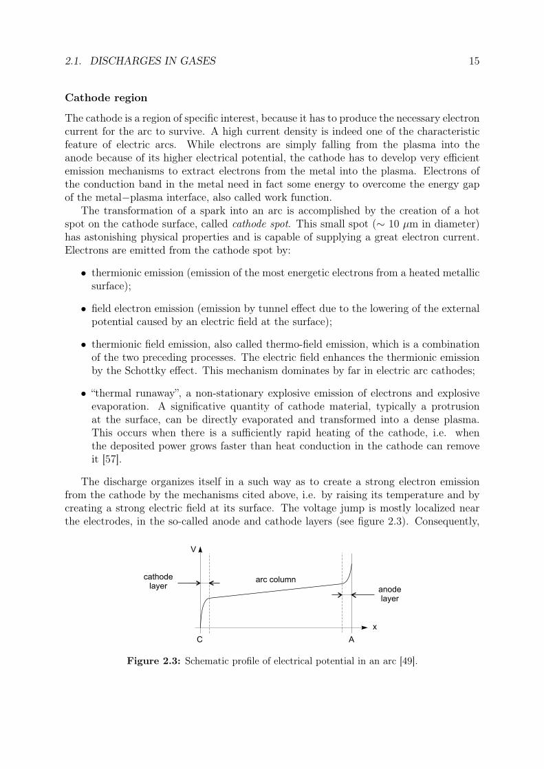
The discharge organizes itself in a such way as to create a strong electron emissionfrom the cathode by the mechanisms cited above, i.e. by raising its temperature and bycreating a strong electric field at its surface. The voltage jump is mostly localized nearthe electrodes, in the so-called anode and cathode layers (see figure 2.3). Consequently,
anodelayer
cathodelayer
arc column
x
V
C A
Figure 2.3: Schematic profile of electrical potential in an arc [49].

16 CHAPTER 2. EDM PLASMAS : BACKGROUND
the electric field is particularly high in these very thin regions. This type of potentialprofile is due to the presence of space charged regions near the electrodes. The plasma inthe cathode layer, usually called cathode spot plasma because it is located in front of thecathode spot, is a small and dense plasma. It remains poorly understood, but its electrontemperature is estimated around 5 eV (60’000 K) and its density around 1020 cm−3. Thecathode spot plasma should thus be dense enough to present non-ideal effects [57].
A detailed structure of the cathode layer is given in figure 2.4. While the plasmaof the arc column is assumed to be in thermal equilibrium, the plasma located in thecathode layer is characterized by deviations from equilibrium [53]. First, a deviation ofthe electron temperature Te from the heavy particles’ temperature Th is present in a layerof thermal relaxation. Then, we have a violation of the ionization equilibrium. In thisionization layer, the production rate of ions is very high due to collisions with energeticelectrons strongly accelerated from the cathode. The ion flux leaving this layer towards thecathode is thus much higher than the flux entering from the layer of thermal relaxation.The dense cathode spot plasma is created in this layer. Finally, the quasineutrality isviolated in a very thin sheath near the cathode, where the ion density n+ is higher thanthe electron density ne. This is the space charged region creating the potential profileshown in figure 2.3, and where almost all the voltage drop is located.
cath
ode
sheath ionization layer layer of thermal relaxation arc column
space charged(n > n )+ e
quasineutral quasineutral
collisionlessionization > recombination ionization = recombination
~ 20 nm(Debye length) ~ 10 mm ~ 100 mm
T > Te h
LocalThermal
Equilibrium(LTE)
e-
+++
e-
+
x
electric potential
+++
Figure 2.4: Schematic structure of the cathode layer (not to scale). The dimensions of thethree layers are evaluated for an argon atmospheric pressure arc plasma at 10’000 K and with acharged particle density of 1017 cm−3 [53].
By this plasma structure, the cathode spot is strongly heated by the ion bombardmentcoming from the ionization layer through the collisionless sheath. This heating leads toevaporation and melting, thermionic emission and thermal runaway in some cases. Theelectron emission is further increased by the electric field produced by the sheath, addingfield emission and thermionic field emission. In return, the electrons coming from thecathode are crucial to create a high ionization rate in the ionization layer, producing
2.1. DISCHARGES IN GASES 17
the ions that will heat the cathode in a self-consistently balanced regime. This coupledion/electron production is the sustaining mechanism of the arc discharge.
The terms involved in the energy balance at the cathode spot are multiple. Theenergy is mainly brought by ion bombardment, but smaller contributions are also givenby Joule heating, atom and electron bombardment, recombination in the cathode, plasmaradiation (almost negligible [57]) and Thomson effect (also negligible). Energy is mostlydissipated by electron emission and heat conduction in the electrode (slow process), butalso by evaporation, surface radiation and droplet emission. The relative importance of allthese energy sources and sinks depend strongly on the arc conditions (pressure, materials,current, etc.). Heating mechanisms of electrodes in EDM sparks should be very similarto those occurring in arcs as described here.
The temperature of a cathode spot is typically around 4’000−5’000 K [57], high abovethe fusion temperatures of metals, which explains the erosive effect of arcs on cathodes.Besides direct evaporation, ejection of cathode melted matter due to the plasma pressureand explosive erosion by thermal runaway, another erosive mechanism can occur also dur-ing the discharge. If energy dissipation dominates at the surface due to a high radiationand electron emission (this is the case if the surface temperature is very high), the maxi-mum temperature is located below the surface, in the cathode spot. This will lead to aninternal explosion, and consequently to ejection of solid or liquid matter into the plasma,in the form of µm droplets [57].
Anode region
At the anode, the situation is also complex, depending strongly on experimental conditionswith several different modes, and not completely understood. Generally, the current isdistributed over a larger surface than at the cathode. The current density is thus lower,and no significative erosion is visible. However, anode spots can develop under certainconditions of current, pressure and anode geometry. In this case, matter can also beevaporated and significant erosion is observed. The plasma structure near the anode hassimilarities with that near the cathode. A negative space charged region is located directlynear the anode surface (ne > n+), because ions are unable to cross the anode potentialbarrier. The metal vapor coming from the anode can thus be ionized in the anode layer,due to this space charged region. Energy is brought to the anode by the electron flux andby recombination with ions in the anode; energy is dissipated through evaporation andheat conduction. The temperature of the anode spot is slightly lower than that of thecathode spot, still being around 3’000 K [49].
Inter-electrode plasma
A large quantity of power is dissipated in the arc column by the Joule effect, heat conduc-tion and radiation. On the axis of the column, the plasma temperature is typically around5 eV (60’000 K) and the electron density around 1016 cm−3, but they depend on the gas,the pressure and the current. These values decrease radially, i.e. towards the edges ofthe column. The plasma of the arc column is thus much less dense than the cathode spotplasma. Due to frequent collisions and thus intensive energy exchange between particles,
18 CHAPTER 2. EDM PLASMAS : BACKGROUND
the plasma of high-pressure arcs is in local thermal equilibrium. The degree of ionizationis also very high, close to 100%.
Arcs in EDM
EDM sparks can sometimes transform into arcs, especially if long discharge durations andgraphite electrodes are used. One hot spot is then created on each electrode surface, andthe following discharges will systematically take place between these two hot spots andinstantly turn into an arc. The result is catastrophic from the erosion point of view, leadingto a localized burn of the workpiece surface and to the destruction of the electrode shape.This is particularly problematic when performing smoothing and polishing operations.Hot spots have to be avoided as much as possible during the EDM process, because oneof the advantages of this technique is precisely to distribute the erosion spots over thewhole workpiece surface. The stochastic change in the localization of the successive sparkdischarges is thus crucial in EDM.
The arcing phenomenon during EDM is well known, and is generally avoided by stop-ping the discharge as soon as the voltage reaches a value below a fixed threshold, typically15−20 V. A decrease in the discharge voltage is the sign of a transition into an arc, becausearcs burn with lower voltage than sparks (see figure 2.1). Other arc detection methodsexist, based on the measurement of the time lag between the voltage application and thebreakdown, on the measurement of the ignition voltage value, or on the measurement ofthe voltage descending flank at the breakdown [58].
2.2 Discharges in dielectric liquids
The principal difference between discharges in gases and discharges in liquids is the den-sity of the medium in which the breakdown occurs. The higher density of liquids makesthem more difficult to break down, i.e. it requires a higher electric field. As describedbelow, the breakdown mechanism is also slightly different, and the plasma properties arestrongly influenced by the pressure imposed by the surrounding liquid.
Breakdown in dielectric liquids have been widely studied, especially for insulationproblems of electric transformers [32]. Published articles on breakdown phenomena inliquids are very numerous, and the existing knowledge is summarized in a few reviewarticles [32, 59–63]. A wide range of liquids have been investigated: water [64], saltedwater solutions [65], oils with different aromatic constituents [30,66,67], silicon fluids [59],liquid argon and nitrogen [31, 68], benzene, toluene, carbon tetrachloride [69], and otherhydrocarbon liquids [70–72] such as propane, pentane, cyclopentene, hexane, cyclohexane,isooctane, decane, etc. The influences of hydrostatic pressure, conductivity [65], viscosity[59], additives [73] and particles [74, 75] on the breakdown mechanism have also beenstudied.
As in high-pressure gases, streamers are involved in breakdown in liquids. Two types ofstreamer exist: the positive streamer starting from the anode, and the negative streamerstarting from the cathode. The use of a point-to-plane geometry permits a separate obser-

2.2. DISCHARGES IN DIELECTRIC LIQUIDS 19
vation of the two types of streamer, depending on the polarity of the electrodes. Contraryto the situation in gases, the structure and propagation speed of positive and negativestreamers are different. As shown in figure 2.5, the positive streamer is “filamentary” and“fast” (∼ 1−10 km/s), and the negative streamer is “bushy” and “slow” (∼ 100 m/s). Inpoint-to-point geometry, the two types of streamer are emitted from both electrodes.
Figure 2.5: Shadowgraphs of negative and positive streamers in oil (taken from [30]).
The sequence of events leading to breakdown can be broken down as follows:
1. Initiation
The initiation of the breakdown mechanism differs from that in gases. Direct prop-agation of electrons into the liquid and impact ionization are difficult, due to thestrong collisions between electrons and molecules occurring in this dense medium.An avalanche of electrons in the liquid phase is thus unlikely, or at least only of shortrange. It is generally accepted that the development of the primary avalanche, whichwill create the streamer, takes place in a region of lower density, created beforehandnear the electrode. If the liquid pressure is not too high, this low density region isa vapor bubble (or a vortex of hot liquid in very viscous liquids [59]).
However, this point is controversial. According to [70, 76], the positive streamerwould be a purely electronic process occurring in the bulk liquid, while negativestreamer would first involve the formation of a bubble. This should explain thedifferent propagation speed of the two types of streamer. On the other hand, otherauthors claim that the breakdown process cannot be initiated without the presenceof bubbles [77, 78]. The effect of the pressure on streamer initiation, for example,is in good agreement with this second theory. Increasing the pressure inhibits infact streamer development and increases the breakdown voltage. This shows thatthe phenomena involved in the breakdown mechanism occur in a gaseous medium.Additional experimental evidence seems to demonstrate that the role of bubbles inthe breakdown triggering is indisputable [79].
Micro-bubbles can pre-exist in the liquid [78] or form electrically, i.e. from heatreleased by small electron avalanches in the liquid or by field emission near electrode

20 CHAPTER 2. EDM PLASMAS : BACKGROUND
asperities [68, 80]. In salted solutions, ionic currents can also slightly enhance theformation of bubbles [62].
2. Streamer formation
The propagation of the primary electron avalanche is strongly facilitated in the bub-ble. Since electrons are continuously heating the liquid in the front of the avalanche,and consequently lowering its density, the bubble is growing (time scale ∼ 10 ns).New avalanches are formed and thus new bubbles grow ahead of the preceding ones.The ionization of a channel in the liquid, i.e. the formation of the streamer, iscaused by this cycle of heating, density lowering and avalanche growth.
3. Streamer propagation
The streamer then grows and propagates according to the mechanism describedabove, governed by a combination of electrostatic and hydrodynamic forces andeven instabilities [32, 59]. This mechanism is quite similar to that in gases, butmore complex. The structure of the streamer is systematically branched, morethan in gases. This reflects the difficulty for the ionization front to propagate in adense medium. It could also be due to other inhomogeneously distributed micro-bubbles leading the streamer path, or due to electrostatic repulsion between adjacentstreamer branches [78]. Small electric currents (in the form of bursts of fast pulses),localized weak light emission and shock waves are associated with the propagationof streamers.
4. Gap completion and breakdown
When the streamer reaches the other electrode, a reverse ionizing front is observedas in gases, starting from the reached electrode and going back towards the initialelectrode. The ionized channel thus thickens, establishing the spark or arc discharge.With negative streamers, the return stroke can even be emitted before the streamerhas reached the anode [76]. Intense emission of light is recorded simultaneously withthe gap completion, as shown in figure 2.6.
This general description of the breakdown mechanism does not take into account theeffects of the numerous experimental parameters. The characteristics of the streamersdepend on the gap voltage and distance, on the electrode materials, geometry and surfacestate, on the liquid pressure, viscosity, density, conductivity, temperature, composition,molecular structure, purity, etc. The presence of particles, for example, strongly facilitatesthe triggering of a breakdown. The contamination of the dielectric is thus as important asits type for the initiation of a breakdown. The addition of so-called “electron scavengers”can also increase the propagation speed of negative streamers by one order of magnitude.This type of additive (e.g. SF6 or C2H5Cl [30]) increases the electronic affinity of thedielectric molecules. Though streamers are of gaseous nature (cf. influence of pressure,shock waves, role of bubbles), this dependence on electron scavenging additives show thatelectronic processes are also operating. The emission of light is another evidence of thisfact.
2.2. DISCHARGES IN DIELECTRIC LIQUIDS 21
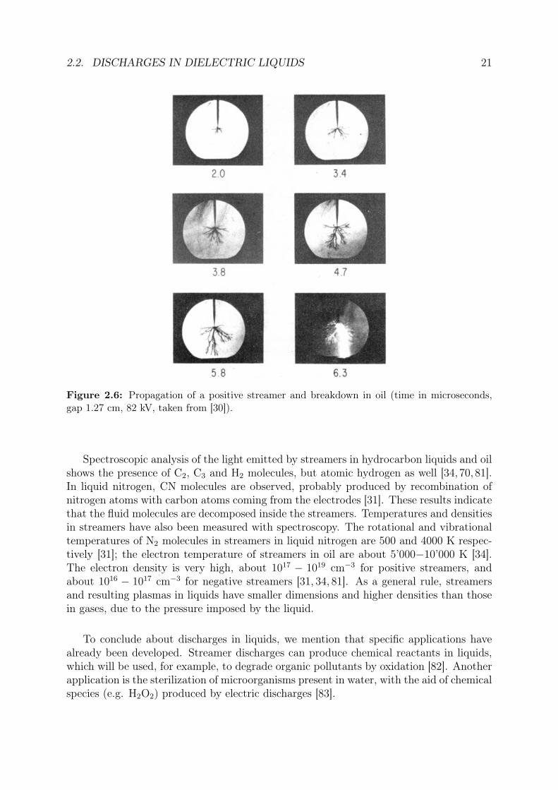
Figure 2.6: Propagation of a positive streamer and breakdown in oil (time in microseconds,gap 1.27 cm, 82 kV, taken from [30]).
Spectroscopic analysis of the light emitted by streamers in hydrocarbon liquids and oilshows the presence of C2, C3 and H2 molecules, but atomic hydrogen as well [34, 70, 81].In liquid nitrogen, CN molecules are observed, probably produced by recombination ofnitrogen atoms with carbon atoms coming from the electrodes [31]. These results indicatethat the fluid molecules are decomposed inside the streamers. Temperatures and densitiesin streamers have also been measured with spectroscopy. The rotational and vibrationaltemperatures of N2 molecules in streamers in liquid nitrogen are 500 and 4000 K respec-tively [31]; the electron temperature of streamers in oil are about 5’000−10’000 K [34].The electron density is very high, about 1017 − 1019 cm−3 for positive streamers, andabout 1016 − 1017 cm−3 for negative streamers [31, 34, 81]. As a general rule, streamersand resulting plasmas in liquids have smaller dimensions and higher densities than thosein gases, due to the pressure imposed by the liquid.
To conclude about discharges in liquids, we mention that specific applications havealready been developed. Streamer discharges can produce chemical reactants in liquids,which will be used, for example, to degrade organic pollutants by oxidation [82]. Anotherapplication is the sterilization of microorganisms present in water, with the aid of chemicalspecies (e.g. H2O2) produced by electric discharges [83].

22 CHAPTER 2. EDM PLASMAS : BACKGROUND
Furthermore, bubbles are of great interest since single-bubble sonoluminescence hasbeen discovered. A gas micro-bubble, trapped in a liquid and periodically driven by intenseacoustic waves, can emit light when it is violently collapsing. This phenomenon is calledsonoluminescence, and still remains puzzling [84]. The emitted light is in the UV range,which implies a high energy density inside the bubble. Recent experiments seem to provethe existence of a plasma inside a sonoluminescing bubble [85]. Its temperature wouldbe above 15’000 K. Thus, these bubbles could possibly be used to produce thermonuclearfusion.
2.3 Other similar plasmas
Besides sparks and high-pressure arcs in gases, other plasmas have similar properties tothose created by electric discharges in dielectric liquids and to EDM plasmas.
Exploding wires
Plasmas in liquids can not only be created by applying high voltage between two im-mersed electrodes. They can also be formed by exploding wires. In such experiments, athin metal wire placed in water is rapidly vaporized due to the flow of a strong current(∼ 100 kA on µs time scale). The plasmas produced in this way have extremely high elec-tron densities (1021− 1022 cm−3) and pressure (∼ 10 kbar), and temperatures of a few eV(10’000−30’000 K) [33,86–88]. These high densities are caused by the strong confinementcreated by the liquid inertia. Such plasmas are so dense that their core is optically highlyopaque. Explosives have even been used to further increase the plasma confinement, andconsequently increase the plasma pressure and density [89].
Capillary discharges
In this type of discharge, the confining medium is a small capillary made of glass oranother dielectric (Teflon, polyethylene, alumina, BeO for example), typically with aninner diameter of 1 mm. This tube is in contact with two electrodes applying a fast currentpulse (∼ 1 kA over 100 ns). The plasma is formed by ablation of the capillary walls. Theelectron densities reached are also high (1016− 1019 cm−3), and the temperatures are of afew eV [35,90–92].
Laser-produced plasmas
Plasmas of metals and alloys can be created by focusing energetic Nd:YAG laser pulseson solid targets, placed in a vacuum chamber. Typical pulses have a power density of1010 W/cm2, a duration of 7 ns, a repetition frequency of 30 Hz, and can be focused on a300 µm diameter spot. These plasmas have an electron density of 1016 − 1018 cm−3, anda temperature of about 1−1.5 eV (10’000−15’000 K) [93–95].
2.3. OTHER SIMILAR PLASMAS 23
Shock waves
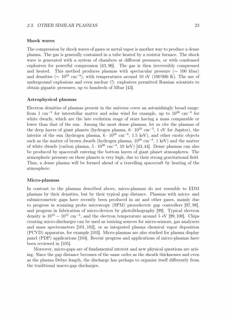
The compression by shock waves of gases or metal vapor is another way to produce a denseplasma. The gas is generally contained in a tube heated by a resistor furnace. The shockwave is generated with a system of chambers at different pressures, or with condensedexplosives for powerful compression [43, 96]. The gas is then irreversibly compressedand heated. This method produces plasmas with spectacular pressure (∼ 100 kbar)and densities (∼ 1023 cm−3), with temperatures around 10 eV (100’000 K). The use ofunderground explosions and even nuclear (!) explosives permitted Russian scientists toobtain gigantic pressures, up to hundreds of Mbar [43].
Astrophysical plasmas
Electron densities of plasmas present in the universe cover an astonishingly broad range:from 1 cm−3 for interstellar matter and solar wind for example, up to 1030 cm−3 forwhite dwarfs, which are the late evolution stage of stars having a mass comparable orlower than that of the sun. Among the most dense plasmas, let us cite the plasmas ofthe deep layers of giant planets (hydrogen plasma, 6 · 1024 cm−3, 1 eV for Jupiter), theinterior of the sun (hydrogen plasma, 6 · 1025 cm−3, 1.5 keV), and other exotic objectssuch as the matter of brown dwarfs (hydrogen plasma, 1028 cm−3, 1 keV) and the matterof white dwarfs (carbon plasma, 5 · 1030 cm−3, 10 keV) [43, 44]. Dense plasmas can alsobe produced by spacecraft entering the bottom layers of giant planet atmospheres. Theatmospheric pressure on these planets is very high, due to their strong gravitational field.Thus, a dense plasma will be formed ahead of a travelling spacecraft by heating of theatmosphere.
Micro-plasmas
In contrast to the plasmas described above, micro-plasmas do not resemble to EDMplasmas by their densities, but by their typical gap distance. Plasmas with micro- andsubmicrometric gaps have recently been produced in air and other gases, mainly dueto progress in scanning probe microscopy (SPM) piezoelectric gap controllers [97, 98],and progress in fabrication of micro-devices by photolithography [99]. Typical electrondensity is 1012 − 1015 cm−3, and the electron temperature around 5 eV [99, 100]. Chipscreating micro-discharges can be used as ionizing sources for micro-sensors, gas analyzersand mass spectrometers [101, 102], or as integrated plasma chemical vapor deposition(PCVD) apparatus, for example [103]. Micro-plasmas are also studied for plasma displaypanel (PDP) applications [104]. Recent progress and applications of micro-plasmas havebeen reviewed in [105].
Moreover, micro-gaps are of fundamental interest and new physical questions are aris-ing. Since the gap distance becomes of the same order as the sheath thicknesses and evenas the plasma Debye length, the discharge has perhaps to organize itself differently fromthe traditional macro-gap discharges.

24 CHAPTER 2. EDM PLASMAS : BACKGROUND
Chapter 3
Experimental setup and diagnostics
The first section of this chapter presents the EDM device used in this work, along withthe machining parameters. The various plasma diagnostics are then described in thefollowing sections. Finally, in the last section we address the specific difficulties relatedto the experimental study of EDM plasmas.
3.1 Electrical discharge machining device
Figure 3.1 presents different views of the machining equipment at the CRPP. We use asmall and versatile die-sinking EDM machine, equipped with a generator of the Roboformtype from Charmilles Technologies. The electrode is cylindrical, with a diameter of 3 or5 mm. In order to better control the localization of the sparks, its tip is conical. Theservo-controlled movement of the electrode is only vertical. The workpiece used in ourexperiments is generally a flat cylinder, 5 cm in diameter. In order to flush the particlescontaminating the electrode gap during machining, the dielectric can be pumped, andre-injected into the gap with a shower. No dielectric cleaning is performed during thisclosed circuit circulation.
The dielectric, the electrode and the workpiece can easily be changed. We use:
• deionized water (typical conductivity 1.5 µS/cm), mineral oil (FluX Elf 2, oil forEDM, viscosity 6) or liquid nitrogen as dielectric. With liquid nitrogen, the work-piece is placed in a dewar to avoid boiling as much as possible;
• electrodes in copper, tungsten, graphite and zinc;
• workpieces in W300 steel (AISI Type H11).
The machining process is completely controlled by the generator. It supplies the dis-charge voltage and current, regulates them, and controls the servomotor for the electrodedisplacement. The generator uses principally the measurement of the gap voltage toregulate and control the process.
25

26 CHAPTER 3. EXPERIMENTAL SETUP AND DIAGNOSTICS
(b)
(c)
(a)
EDM pulsegenerator
electric motor(for servo-controlled
electrode displacement)
pump
dielectricshower
electrode
workpiece
fibre optics (foroptical diagnostics)
dielectric circuit
EDM machine
control
Figure 3.1: EDM device. (a) General view; (b) EDM machine; (c) electrodes.
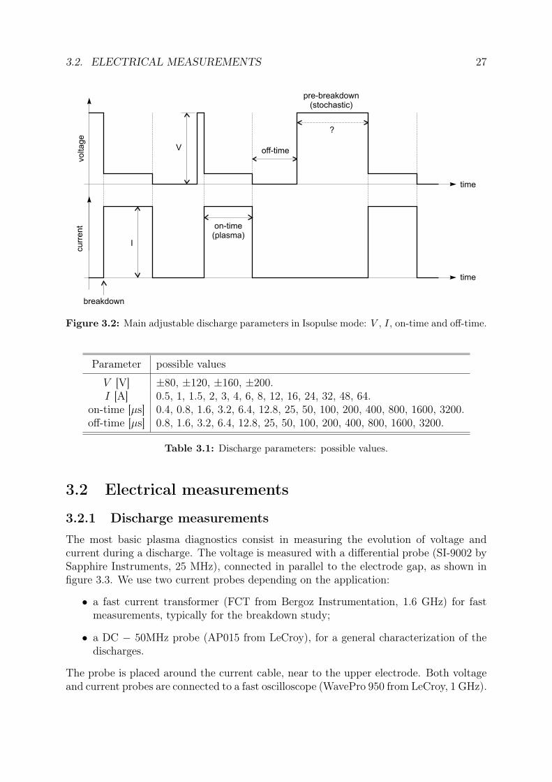
Figure 3.2 shows the discharge parameters which can be set with the generator: igni-tion voltage V , discharge current I, discharge on-time, off-time (pause between the endof a discharge and the voltage rise for the next one), electrode polarity.
It is impossible to control the pre-breakdown duration, i.e. the time lag between thevoltage application and the breakdown, because it depends on the electrode gap and onphysico-chemical properties of the dielectric. Note that the pre-breakdown duration is alsocalled “ignition delay time” or “breakdown time lag”. The value of the voltage during thedischarge can not be set by the generator either. Its value depends on electrode materials,but is typically around 20−25 V. The values that we can choose with our generator forV , I, on-time and off-time are given in table 3.1.
The machining mode schematically presented in figure 3.2 is called Isopulse, becauseevery discharge has the same on-time, independently of the pre-breakdown duration. Thismode is the standard machining mode used in this work. By adding a capacitor in parallelto the gap, it is possible to use the generator in a capacitive mode, generally used for surfacefinishing [106]. The sparks are produced by successive discharges of the capacitor. In thismode, the polarity is always chosen negative. The discharge on-time and current are notcontrolled, and thus can slightly vary from a discharge to the other, in contrary to theIsopulse mode. Typically, with a 10 nF capacitor, the discharge duration is around 1.5 µsand the current around 6 A.
3.2. ELECTRICAL MEASUREMENTS 27
voltage
curr
ent on-time
(plasma)
off-time
time
pre-breakdown(stochastic)
?
breakdown
I
V
time
Figure 3.2: Main adjustable discharge parameters in Isopulse mode: V , I, on-time and off-time.
Parameter possible values
V [V] ±80, ±120, ±160, ±200.I [A] 0.5, 1, 1.5, 2, 3, 4, 6, 8, 12, 16, 24, 32, 48, 64.
on-time [µs] 0.4, 0.8, 1.6, 3.2, 6.4, 12.8, 25, 50, 100, 200, 400, 800, 1600, 3200.off-time [µs] 0.8, 1.6, 3.2, 6.4, 12.8, 25, 50, 100, 200, 400, 800, 1600, 3200.
Table 3.1: Discharge parameters: possible values.
3.2 Electrical measurements
3.2.1 Discharge measurements
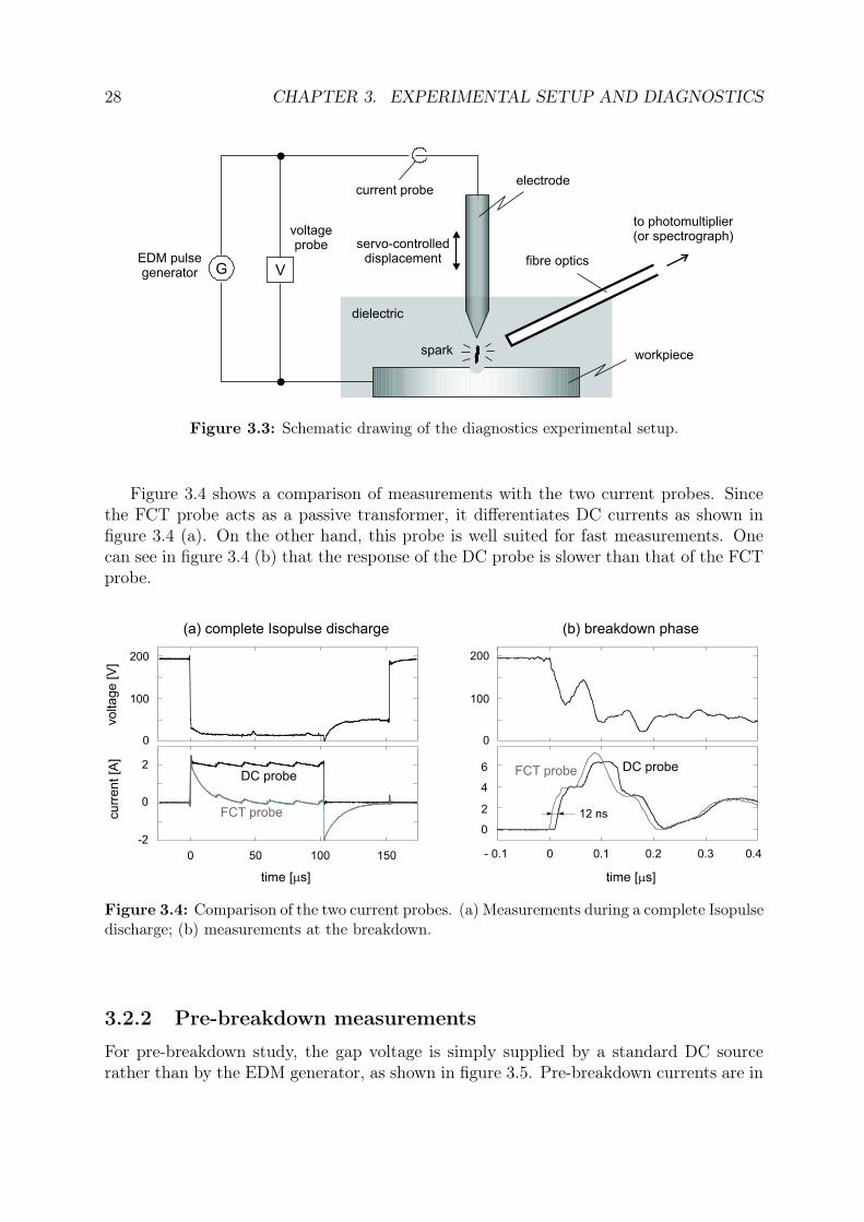
The most basic plasma diagnostics consist in measuring the evolution of voltage andcurrent during a discharge. The voltage is measured with a differential probe (SI-9002 bySapphire Instruments, 25 MHz), connected in parallel to the electrode gap, as shown infigure 3.3. We use two current probes depending on the application:
• a fast current transformer (FCT from Bergoz Instrumentation, 1.6 GHz) for fastmeasurements, typically for the breakdown study;
• a DC − 50MHz probe (AP015 from LeCroy), for a general characterization of thedischarges.
The probe is placed around the current cable, near to the upper electrode. Both voltageand current probes are connected to a fast oscilloscope (WavePro 950 from LeCroy, 1 GHz).
28 CHAPTER 3. EXPERIMENTAL SETUP AND DIAGNOSTICS
workpiece
electrode
fibre optics
dielectric
spark
EDM pulsegenerator G
voltageprobe
current probe
V
to photomultiplier(or spectrograph)
servo-controlleddisplacement
Figure 3.3: Schematic drawing of the diagnostics experimental setup.
Figure 3.4 shows a comparison of measurements with the two current probes. Sincethe FCT probe acts as a passive transformer, it differentiates DC currents as shown infigure 3.4 (a). On the other hand, this probe is well suited for fast measurements. Onecan see in figure 3.4 (b) that the response of the DC probe is slower than that of the FCTprobe.
0
100
200
-2
0
2
0 50 100 150
time [ s]m
0
2
4
6
0 0.1 0.2 0.3 0.4
voltage [V
]curr
ent [A
]
0
100
200
- 0.1
time [ s]m
FCT probe
DC probe FCT probe DC probe
12 ns
(a) complete Isopulse discharge (b) breakdown phase
Figure 3.4: Comparison of the two current probes. (a) Measurements during a complete Isopulsedischarge; (b) measurements at the breakdown.
3.2.2 Pre-breakdown measurements
For pre-breakdown study, the gap voltage is simply supplied by a standard DC sourcerather than by the EDM generator, as shown in figure 3.5. Pre-breakdown currents are in
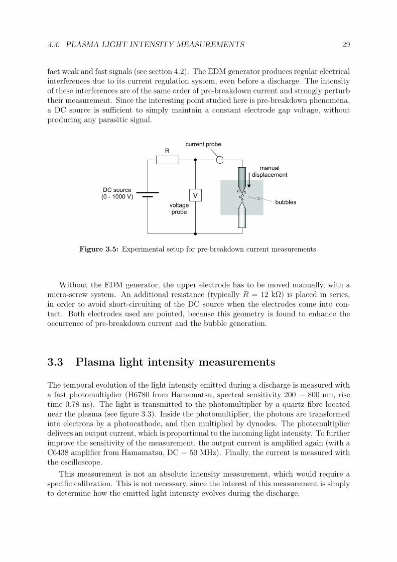
3.3. PLASMA LIGHT INTENSITY MEASUREMENTS 29
fact weak and fast signals (see section 4.2). The EDM generator produces regular electricalinterferences due to its current regulation system, even before a discharge. The intensityof these interferences are of the same order of pre-breakdown current and strongly perturbtheir measurement. Since the interesting point studied here is pre-breakdown phenomena,a DC source is sufficient to simply maintain a constant electrode gap voltage, withoutproducing any parasitic signal.
R
DC source(0 - 1000 V)
manualdisplacement
voltageprobe
current probe
Vbubbles
Figure 3.5: Experimental setup for pre-breakdown current measurements.
Without the EDM generator, the upper electrode has to be moved manually, with amicro-screw system. An additional resistance (typically R = 12 kΩ) is placed in series,in order to avoid short-circuiting of the DC source when the electrodes come into con-tact. Both electrodes used are pointed, because this geometry is found to enhance theoccurrence of pre-breakdown current and the bubble generation.
3.3 Plasma light intensity measurements
The temporal evolution of the light intensity emitted during a discharge is measured witha fast photomultiplier (H6780 from Hamamatsu, spectral sensitivity 200 − 800 nm, risetime 0.78 ns). The light is transmitted to the photomultiplier by a quartz fibre locatednear the plasma (see figure 3.3). Inside the photomultiplier, the photons are transformedinto electrons by a photocathode, and then multiplied by dynodes. The photomultiplierdelivers an output current, which is proportional to the incoming light intensity. To furtherimprove the sensitivity of the measurement, the output current is amplified again (with aC6438 amplifier from Hamamatsu, DC − 50 MHz). Finally, the current is measured withthe oscilloscope.
This measurement is not an absolute intensity measurement, which would require aspecific calibration. This is not necessary, since the interest of this measurement is simplyto determine how the emitted light intensity evolves during the discharge.
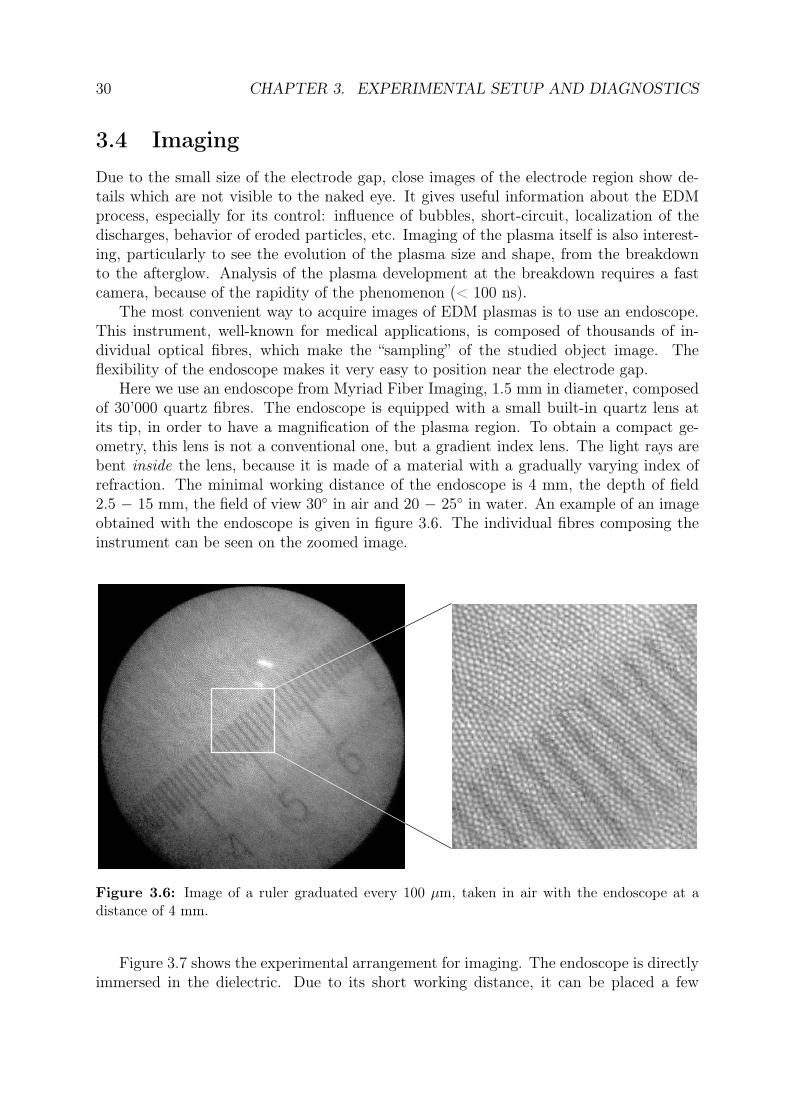
30 CHAPTER 3. EXPERIMENTAL SETUP AND DIAGNOSTICS
3.4 ImagingDue to the small size of the electrode gap, close images of the electrode region show de-tails which are not visible to the naked eye. It gives useful information about the EDMprocess, especially for its control: influence of bubbles, short-circuit, localization of thedischarges, behavior of eroded particles, etc. Imaging of the plasma itself is also interest-ing, particularly to see the evolution of the plasma size and shape, from the breakdownto the afterglow. Analysis of the plasma development at the breakdown requires a fastcamera, because of the rapidity of the phenomenon (< 100 ns).
The most convenient way to acquire images of EDM plasmas is to use an endoscope.This instrument, well-known for medical applications, is composed of thousands of in-dividual optical fibres, which make the “sampling” of the studied object image. Theflexibility of the endoscope makes it very easy to position near the electrode gap.
Here we use an endoscope from Myriad Fiber Imaging, 1.5 mm in diameter, composedof 30’000 quartz fibres. The endoscope is equipped with a small built-in quartz lens atits tip, in order to have a magnification of the plasma region. To obtain a compact ge-ometry, this lens is not a conventional one, but a gradient index lens. The light rays arebent inside the lens, because it is made of a material with a gradually varying index ofrefraction. The minimal working distance of the endoscope is 4 mm, the depth of field2.5 − 15 mm, the field of view 30 in air and 20 − 25 in water. An example of an imageobtained with the endoscope is given in figure 3.6. The individual fibres composing theinstrument can be seen on the zoomed image.
Figure 3.6: Image of a ruler graduated every 100 µm, taken in air with the endoscope at adistance of 4 mm.
Figure 3.7 shows the experimental arrangement for imaging. The endoscope is directlyimmersed in the dielectric. Due to its short working distance, it can be placed a few

3.4. IMAGING 31
millimeters from the spark, assuring therefore a good image magnification and small lightabsorption by the dielectric. When studying the EDM process in general, the endoscopeis placed a few centimeters from the electrode gap and slightly above, in order to havea general view of the electrodes and their surrounding environment. To observe theelectrodes, an external lighting is necessary to illuminate them, because our endoscope isnot equipped with a source for illumination. We use two halogen lamps for this purpose.For plasma imaging, the endoscope is placed much closer to the plasma (5 mm typically),and the flat workpiece is replaced by a pointed one. With this point-to-point geometry,the plasma is thus localized as much as possible.
endoscope
(a) (b)to camera
lens
Figure 3.7: Schematic drawing of the experimental setup for imaging. (a) Imaging of the EDMprocess; (b) plasma imaging.
The endoscope is directly connected to a CCD camera (SensiCam Fast Shutter fromPCO Imaging, 12 bit, exposure time 100 ns − 10 ms, 1280 × 768 pixels). The imagefocusing is done by a lens with adjustable focal length, placed between the end of theendoscope and the CCD camera.
For time-resolved imaging, i.e. acquisition of successive images of short exposure timetaken at different moments of the discharge, the camera can be gated. In this mode,the exposure begins with an external trigger signal, produced by a pulse generator. Thedelay between the breakdown (t = 0) and the beginning of the exposure is set by the pulsegenerator. The t = 0 trigger is obtained by measuring the current rise or the voltage dropwhich occur at the breakdown.
For fast imaging, we use another camera, an intensified CCD camera (ICCD PI-MAXcamera from Princeton Instruments, 16 bit, < 2 ns gating, 1024 × 1024 pixels). Sinceshort exposure time implies low measured intensities, light intensification is required.This is performed in ICCD cameras by a micro-channel plate (MCP) placed just behinda photocathode. The electrons created in the photocathode are multiplied in the MCP,and then re-transformed into photons by a fluorescent screen. The MCP is also used as ashutter for gated exposure. Since the electrons in the MCP can be abruptly blocked byreversing the electric field, fast gating is achievable with ICCD cameras. For time-resolvedimaging with the PI-MAX camera, the delay from the breakdown can be set without apulse generator. The t = 0 trigger is directly sent to the camera controller, and the delayis set by software.
32 CHAPTER 3. EXPERIMENTAL SETUP AND DIAGNOSTICS
3.5 Optical emission spectroscopy
Optical emission spectroscopy (OES) is a classical plasma diagnostic. Several impor-tant plasma measurements can be performed with this non-intrusive method: chem-ical composition, temperatures, densities, electric and magnetic fields present in theplasma [107–109].
3.5.1 Principles
OES consists in the spectral analysis of the light emitted in the visible region by theplasma. The light is dispersed in a spectrograph, generally by a grating, and detected byphotodiodes, a photomultiplier or a CCD camera.
Atoms, ions and molecules emit light with a discrete spectrum when they pass froman excited state to a state of lower energy, i.e. when an electron makes a transition froman upper energy level Ei to a lower energy level Ej inside the atom, ion or molecule. Thewavelength λ of the spectral line emitted during this transition will be
λ =hc
Ei − Ej
, (3.1)
where h is Planck’s constant and c the speed of light. Since the atomic or molecularquantum energy levels are different for every element or molecule, the discrete spectrumemitted by these electronic transitions, called bound-bound transitions, is like a charac-teristic signature of the emitting species. The plasma composition can thus be determinedwith OES by identifying the different emitted spectral lines.
While the wavelength of a spectral line is only determined by the type of the emittingspecies, the intensity of this line depends on the abundance of the emitter, i.e. on itsdensity, and also on the population of the excited state considered. This means that lineintensities are dependent on the plasma temperature.
The energy levels of the hydrogen atom can be exactly calculated with quantum me-chanics. The main levels are the eigenvalues of the Hamiltonian describing the electronof the hydrogen atom, and are given by
En = −13.6 eVn2
, n = 1, 2, 3 ... (3.2)
The energy E = 0 corresponds to the ionization threshold. A special terminology is usedfor the lines emitted by atomic hydrogen. They are given in figure 3.8.
A plasma can also emit light with a continuous spectrum. This occurs when freeelectrons recombine in atoms or molecules: they pass from a state E > 0 in the energycontinuum (i.e. with no defined energy) to a discrete level inside an atom or a molecule.These transitions are called free-bound transitions. Continuous light is also emitted whenfree electrons lose energy by passing near an ion or an atom. This is the well-knownBremsstrahlung, or free-free radiation.

3.5. OPTICAL EMISSION SPECTROSCOPY 33
Balmer series Paschen seriesLyman series
- 13.6
- 3.39
- 1.51
- 0.85- 0.54
0
n=1
n=2
n=3
n=4n=5
∞
eV
Hα Hβ Hγ
Lα Lβ Lγ
Pα Pβ
Lδ
…
…
…
…
Figure 3.8: Main quantum levels and emission lines of the hydrogen atom.
3.5.2 Electron temperature measurement
To determine the different temperatures of the species present in a plasma, several spec-troscopic methods exist [107, 108]. In practice, their respective applicability depends onthe type of spectrum emitted by the plasma studied: atomic lines, ionic lines, molecularbands, continuum emission... Most of these methods require the assumption of thermalequilibrium, or at least of local thermal equilibrium (LTE). They need a theoretical re-lation between the populations of the various excited states and the temperature or thepressure, for example. In case of LTE, this relation is simply given by equilibrium statis-tical mechanics or thermodynamics. In case of non-equilibrium plasmas, it is much morecomplicated to develop a theoretical model.
Here, for the electron temperature determination in EDM plasmas, we use the two-linemethod. This method, which is a particular case of the Boltzmann plot method, is basedon measurements of the intensity ratio of two spectral lines, emitted by atoms or ions ofthe same element [107, 108]. Since it is a relative and not an absolute intensity measure-ment, the calibration of the absolute spectral sensitivity of the optical arrangement is notnecessary.
If we assume that the plasma is in a state of LTE (the validity of this assumption forEDM plasmas will be discussed later, in § 6.1.7), the distribution of atoms and ions inthe different excited states is described by the Boltzmann distribution. Thus, the densityni of a certain type particle, atom or ion, in an excited state i is given by
ni =n0 gi
Z· exp
(− Ei
kB Te
), (3.3)
where n0 is the total density of the considered particles in the plasma, gi the statistical

34 CHAPTER 3. EXPERIMENTAL SETUP AND DIAGNOSTICS
weight of the excited level and Ei its energy, Z the partition function, kB the Boltzmannconstant and Te the electron temperature. In case of LTE, Te is also equal to the iontemperature and to the gas temperature; Te could thus be replaced in (3.3) with a uniqueplasma temperature T .
The emission coefficient ε of the line emitted by the transition from the upper state ito a lower state j is
ε =1
4π· hc
λ· Aij ni , (3.4)
where λ is the line wavelength and Aij the probability for the transition from the state ito the state j. Replacing ni by its expression given in (3.3), we obtain
ε =hc
4π· n0
Z· gi Aij
λ· exp
(− Ei
kB Te
).
Considering now two lines λ1 and λ2 emitted by the same species, i.e. by atoms oreven charged ions of the same element, the ratio of their intensities is given by
I1
I2
=ε1
ε2
=g1 A1
λ1
· λ2
g2 A2
· exp
(E2 − E1
kB Te
),
where gi, Aij and Ei for the line k (k = 1, 2) are noted gk, Ak and Ek respectively.Extracting Te from the preceding equation, we finally obtain
Te =E2 − E1
kB
·[
ln
(I1 λ1 g2 A2
I2 λ2 g1 A1
) ]−1
. (3.5)
The ratio I1/I2 is experimentally determined from an emission spectrum. The electrontemperature can be thus calculated with equation (3.5) if Ek, λk, gk and Ak are knownvalues for the two lines.
Practically, the choice of the two lines is of importance. Since the relative error on thetemperature is
∆Te
Te
=kB Te
|E2 − E1| ·∆ (I1/I2)
I1/I2
according to (3.5), it is crucial to choose two lines with a difference |E2 − E1| as largeas possible. Moreover, the chosen lines have to be intense and isolated from other lines,in order to avoid overlapping and to minimize ∆ (I1/I2). It is also desirable that λ1
and λ2 are close to each other. In this case, the absorption by the dielectric and thespectral sensitivity of the optical arrangement can be considered equal for the two lines.No spectral correction is then required for the calculation of I1/I2. Finally, the lines haveto be non-resonant ones, to avoid self-absorption. It has to be emphasized that with thetwo-line method, a minimum error of 10% on Te is expected [107].

3.5. OPTICAL EMISSION SPECTROSCOPY 35
As we will see in chapter 6, copper lines are emitted by EDM plasmas when usinga copper electrode. Three atomic copper lines fulfil the conditions cited above. Theirparameters are given in table 3.2. Since |E2 − E1| must be large, we can use the pairs(a)−(b) and (a)−(c) for the determination of Te with the two-line method.
Line λ [nm] upper state (i) lower state (j) Ei [eV] Ej [eV] gi gj Aij [108s−1]
(a) 510.554 4p 2P3/2 4s2 2D5/2 3.817 1.389 4 6 0.02(b) 515.324 4d 2D3/2 4p 2P1/2 6.191 3.786 4 2 0.6(c) 521.820 4d 2D5/2 4p 2P3/2 6.192 3.817 6 4 0.75
Table 3.2: Line parameters of the Cu I lines used for electron temperature determination [110].
In practice, to calculate the line intensities from a spectrum, the background has to besubtracted first. Then the line shapes are fitted with Lorentzian functions (see § 3.5.3),and eventually deconvolved if there are adjacent lines. The line intensity I is not simplythe maximum value of the peak, but the whole area under the Lorentzian fit.
3.5.3 Electron density measurement
With the electron temperature Te, the electron density ne is another important physicalparameter characterizing a plasma, which can also be determined with optical emissionspectroscopy. Again, there are several methods based on measurements of line and con-tinuum intensities, but also on measurements of line profile [107, 108, 111]. The electrondensity has in fact a direct influence on line shapes, while they are relatively insensitiveto electron and ion temperatures. Spectral lines are broadened and shifted from theirtheoretical position, increasingly with the electron density. The influence of the densityon line broadening can be qualitatively explained as follows: the collision frequency willincrease with density, and so the lifetime of atoms in excited states will decrease due tocollisions. By the Heisenberg principle, this will increase the uncertainty on the energylevels, i.e. the uncertainty on the emitted wavelength. Spectral lines are thus more broad-ened in a dense plasma.
There are several broadening mechanisms:
• the natural broadening, due to the finiteness of the lifetime of an atom in an excitedstate;
• the broadening due to collisions, such as:
– the pressure broadening, caused by collisions between emitters and neutralatoms or molecules;
– the Stark broadening, caused by collisions between emitters and charged per-turbers. The atomic quantum levels of emitters are modified by the Starkeffect, due to the electric field created by the colliding ions or electrons;
36 CHAPTER 3. EXPERIMENTAL SETUP AND DIAGNOSTICS
• the Doppler broadening, due to the thermal movements of the emitters along theline of sight.
Stark broadened lines are experimentally valuable for the density determination, be-cause the Stark broadening is particularly sensitive to the electron density. In a denseplasma, and this is the case of EDM plasmas as we will see in chapter 6, this broadeningmechanism will dominate by far all the others [34, 111]. For more details on the Starkeffect and its consequences on line emission, see appendix A.
The Doppler broadening leads to a Gaussian line shape, while processes involving par-ticle impacts, such as the Stark broadening, lead to a line shape close to a Lorentzian. Ifboth effects take place, the line profile will be a Voigt profile, i.e. a combination of thetwo. Since Stark broadening prevails in EDM plasmas, our lines have a shape close to aLorentzian.
In our case, we use the Hα line emitted by atomic hydrogen at 656.28 nm to deter-mine the electron density. Along with Hβ, this line is a classical candidate for densitymeasurement, because the hydrogen atom is particularly sensitive to the Stark effect.Furthermore, Stark broadening and shift of the hydrogen Balmer lines have been wellstudied since many years, because this type of diagnostic is particularly important infusion experiments and astrophysics, for example. Thus, numerous theoretical and ex-perimental works have been published about Stark broadening and shift of the Hα line,especially for electron density calculations from full width at half maximum (FWHM)measurements [112–115] and from shift measurements [113–117].
Computation of spectral lineshapes is quite difficult, because collisions of both elec-trons and ions with the emitter have to be taken into account as the broadening mecha-nism. But in recent years progress has been made to include several dynamic effects incalculations, especially ion dynamics. Here we used the theories of Gigosos and Cardenosoon broadening [112] and of Oks on shift [115] to calculate the electron density.
Figures 3.9 (a) and (b) show respectively the simulation results for the dependence ofthe FWHM and of the shift of Hα on the electron density. Though the plasma temperaturehas a weak influence on the line profile, the simulations of FWHM are calculated fordifferent temperatures and for different reduced mass µ of the emitter−perturbing particlepair. Here, we use the calculation for a plasma of 10’000 K (which is close to the actualEDM plasma temperature, see chapter 6), and with µ = 1 (i.e. hydrogen atoms perturbedby heavy particles). For the shift simulation, we use calculations made for plasmas withtemperatures from 13’000 to 20’000 K. EDM plasmas are cooler, but simulation resultsfor lower temperature are not available. The determination of ne is more precise with theFWHM measurements, because the broadening of Hα is experimentally easily measurablefor densities at which the shift is still very low. At 5 · 1017 cm−3 for example, the FWHMis 3 nm but the shift is only 1.7 Å.
By fitting the simulation results of the figure 3.9, we obtain two equations giving theelectron density as a function of the Hα FWHM and of the Hα shift. Thus, to calculatene from our FWHM and shift measurements, we use the following relations:
ne = 8.8308 · 1016 · (∆λW
)1.6005 (3.6)
3.5. OPTICAL EMISSION SPECTROSCOPY 37
1014
1016
1018
0.01 0.1 1 10
FWHM of the H line [nm]a
ele
ctro
n d
ensi
ty [
cm]
-3
simulationfit
1018
2·1018
3 1018
·
4 1018
·
5 1018
·
5 10 15 20
shift [Å]of the H linea
simulationfit
ele
ctro
n d
ensi
ty [cm
]-3
(a) broadening (b) shift
Figure 3.9: Relation between the electron density and: (a) the full width at half maximum(FWHM) of the Hα line (simulation results for a 10’000 K plasma with µ = 1, according to [112]);(b) the shift of the Hα line (simulation results for plasmas from 13’000 to 20’000 K, according toOks [115]).
with ne in cm−3 and the FWHM ∆λW in nm, and
ne = 1017 · (1.3591 + 2.0757 ·∆λS + 0.0037 ·∆λ2S) (3.7)
with ne in cm−3 and the shift ∆λS in Å.In practice, we have to take into account the broadening caused by the spectrograph.
This experimental broadening is measured with a laser, which theoretically emits a singlewavelength. The Hα line is treated as the copper lines for Te determination: backgroundsubtraction and Lorentzian fit. Then, the line FWHM is obtained by subtracting theexperimental broadening from the FWHM of the Lorentzian fit.
3.5.4 General experimental setup
The general experimental setup for OES is presented in figure 3.10. The emitted light iscollected by a quartz fibre, 1 mm in diameter. The fibre is immersed in the dielectric,located a few millimeters from the spark to optimize the collected light intensity andto reduce absorption from the dielectric. The light is then dispersed by a spectrographequipped with gratings, and detected by a CCD camera or photodiodes. Finally, thesignal is digitalized and treated with a computer.
We use different spectrographs and detectors depending on the application:
• for time-integrated spectroscopy, a 0.275 m spectrograph (SpectraPro 275 fromActon Research Company) with three gratings (150, 600 and 1200 grooves/mm),
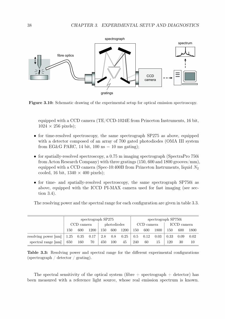
38 CHAPTER 3. EXPERIMENTAL SETUP AND DIAGNOSTICS
spectrum
CCDcamera
fibre optics
spectrograph
gratings
Figure 3.10: Schematic drawing of the experimental setup for optical emission spectroscopy.
equipped with a CCD camera (TE/CCD-1024E from Princeton Instruments, 16 bit,1024 × 256 pixels);
• for time-resolved spectroscopy, the same spectrograph SP275 as above, equippedwith a detector composed of an array of 700 gated photodiodes (OMA III systemfrom EG&G PARC, 14 bit, 100 ns − 10 ms gating);
• for spatially-resolved spectroscopy, a 0.75 m imaging spectrograph (SpectraPro 750ifrom Acton Research Company) with three gratings (150, 600 and 1800 grooves/mm),equipped with a CCD camera (Spec-10:400B from Princeton Instruments, liquid N2
cooled, 16 bit, 1340 × 400 pixels);
• for time- and spatially-resolved spectroscopy, the same spectrograph SP750i asabove, equipped with the ICCD PI-MAX camera used for fast imaging (see sec-tion 3.4).
The resolving power and the spectral range for each configuration are given in table 3.3.
spectrograph SP275 spectrograph SP750iCCD camera photodiodes CCD camera ICCD camera
150 600 1200 150 600 1200 150 600 1800 150 600 1800
resolving power [nm] 1.25 0.35 0.17 2.8 0.8 0.25 0.5 0.12 0.03 0.33 0.09 0.02spectral range [nm] 650 160 70 450 100 45 240 60 15 120 30 10
Table 3.3: Resolving power and spectral range for the different experimental configurations(spectrograph / detector / grating).
The spectral sensitivity of the optical system (fibre + spectrograph + detector) hasbeen measured with a reference light source, whose real emission spectrum is known.
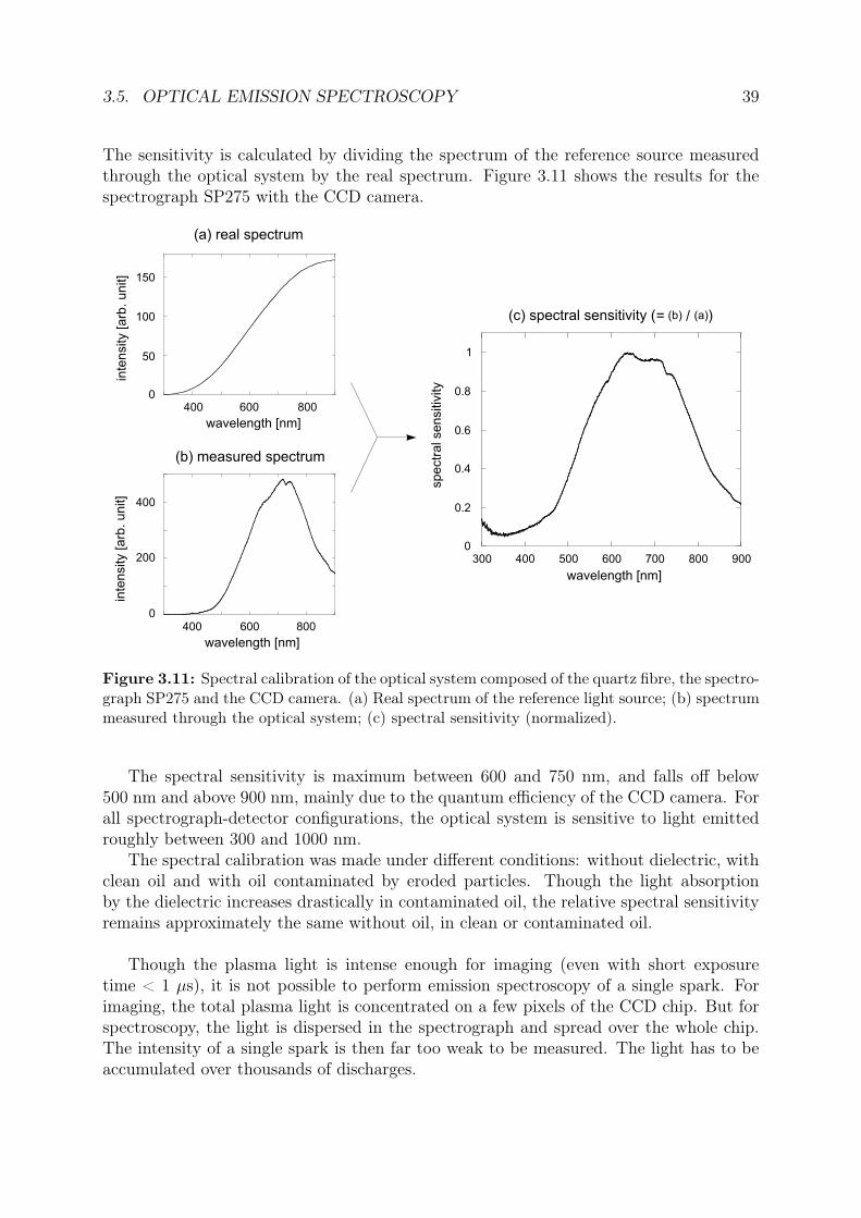
3.5. OPTICAL EMISSION SPECTROSCOPY 39
The sensitivity is calculated by dividing the spectrum of the reference source measuredthrough the optical system by the real spectrum. Figure 3.11 shows the results for thespectrograph SP275 with the CCD camera.
0
50
100
150
400 600 800
wavelength [nm]
inte
nsity [arb
. unit]
(a) real spectrum
0
200
400
400 600 800
wavelength [nm]
inte
nsity [arb
. unit]
(b) measured spectrum
0
0.2
0.4
0.6
0.8
1
300 400 500 600 700 800 900
wavelength [nm]
spectr
al sen
sitiv
ity
(c) spectral sensitivity ( )(b) (a)= /
Figure 3.11: Spectral calibration of the optical system composed of the quartz fibre, the spectro-graph SP275 and the CCD camera. (a) Real spectrum of the reference light source; (b) spectrummeasured through the optical system; (c) spectral sensitivity (normalized).
The spectral sensitivity is maximum between 600 and 750 nm, and falls off below500 nm and above 900 nm, mainly due to the quantum efficiency of the CCD camera. Forall spectrograph-detector configurations, the optical system is sensitive to light emittedroughly between 300 and 1000 nm.
The spectral calibration was made under different conditions: without dielectric, withclean oil and with oil contaminated by eroded particles. Though the light absorptionby the dielectric increases drastically in contaminated oil, the relative spectral sensitivityremains approximately the same without oil, in clean or contaminated oil.
Though the plasma light is intense enough for imaging (even with short exposuretime < 1 µs), it is not possible to perform emission spectroscopy of a single spark. Forimaging, the total plasma light is concentrated on a few pixels of the CCD chip. But forspectroscopy, the light is dispersed in the spectrograph and spread over the whole chip.The intensity of a single spark is then far too weak to be measured. The light has to beaccumulated over thousands of discharges.
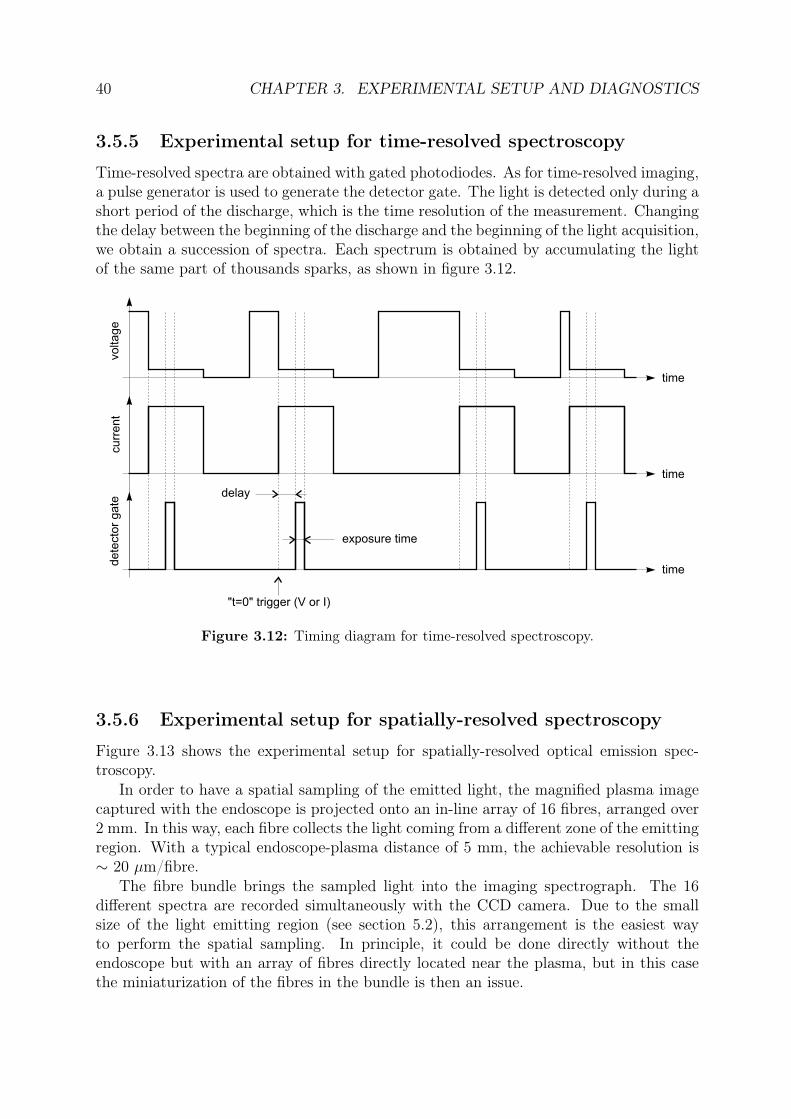
40 CHAPTER 3. EXPERIMENTAL SETUP AND DIAGNOSTICS
3.5.5 Experimental setup for time-resolved spectroscopy
Time-resolved spectra are obtained with gated photodiodes. As for time-resolved imaging,a pulse generator is used to generate the detector gate. The light is detected only during ashort period of the discharge, which is the time resolution of the measurement. Changingthe delay between the beginning of the discharge and the beginning of the light acquisition,we obtain a succession of spectra. Each spectrum is obtained by accumulating the lightof the same part of thousands sparks, as shown in figure 3.12.
delay
exposure time
voltage
curr
ent
dete
cto
r gate
time
"t=0" trigger (V or I)
time
time
Figure 3.12: Timing diagram for time-resolved spectroscopy.
3.5.6 Experimental setup for spatially-resolved spectroscopy
Figure 3.13 shows the experimental setup for spatially-resolved optical emission spec-troscopy.
In order to have a spatial sampling of the emitted light, the magnified plasma imagecaptured with the endoscope is projected onto an in-line array of 16 fibres, arranged over2 mm. In this way, each fibre collects the light coming from a different zone of the emittingregion. With a typical endoscope-plasma distance of 5 mm, the achievable resolution is∼ 20 µm/fibre.
The fibre bundle brings the sampled light into the imaging spectrograph. The 16different spectra are recorded simultaneously with the CCD camera. Due to the smallsize of the light emitting region (see section 5.2), this arrangement is the easiest wayto perform the spatial sampling. In principle, it could be done directly without theendoscope but with an array of fibres directly located near the plasma, but in this casethe miniaturization of the fibres in the bundle is then an issue.
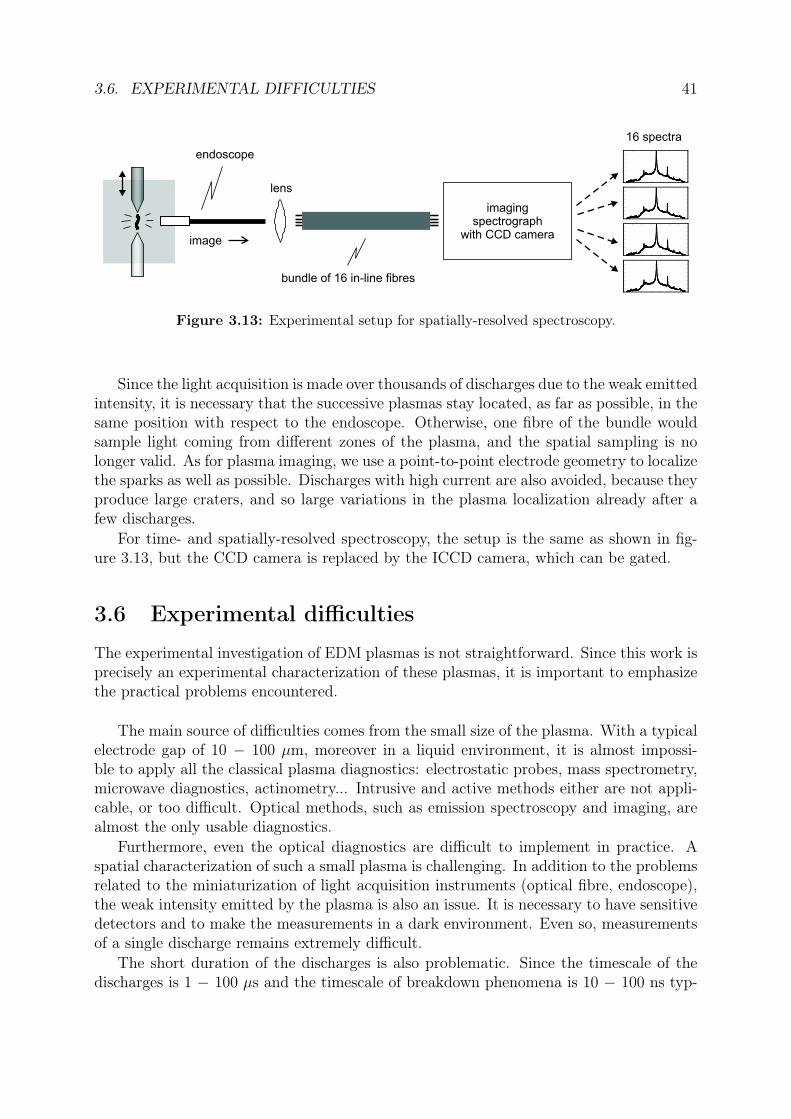
3.6. EXPERIMENTAL DIFFICULTIES 41
endoscope
16 spectra
image
lens
bundle of 16 in-line fibres
imagingspectrograph
with CCD camera
Figure 3.13: Experimental setup for spatially-resolved spectroscopy.
Since the light acquisition is made over thousands of discharges due to the weak emittedintensity, it is necessary that the successive plasmas stay located, as far as possible, in thesame position with respect to the endoscope. Otherwise, one fibre of the bundle wouldsample light coming from different zones of the plasma, and the spatial sampling is nolonger valid. As for plasma imaging, we use a point-to-point electrode geometry to localizethe sparks as well as possible. Discharges with high current are also avoided, because theyproduce large craters, and so large variations in the plasma localization already after afew discharges.
For time- and spatially-resolved spectroscopy, the setup is the same as shown in fig-ure 3.13, but the CCD camera is replaced by the ICCD camera, which can be gated.
3.6 Experimental difficulties
The experimental investigation of EDM plasmas is not straightforward. Since this work isprecisely an experimental characterization of these plasmas, it is important to emphasizethe practical problems encountered.
The main source of difficulties comes from the small size of the plasma. With a typicalelectrode gap of 10 − 100 µm, moreover in a liquid environment, it is almost impossi-ble to apply all the classical plasma diagnostics: electrostatic probes, mass spectrometry,microwave diagnostics, actinometry... Intrusive and active methods either are not appli-cable, or too difficult. Optical methods, such as emission spectroscopy and imaging, arealmost the only usable diagnostics.
Furthermore, even the optical diagnostics are difficult to implement in practice. Aspatial characterization of such a small plasma is challenging. In addition to the problemsrelated to the miniaturization of light acquisition instruments (optical fibre, endoscope),the weak intensity emitted by the plasma is also an issue. It is necessary to have sensitivedetectors and to make the measurements in a dark environment. Even so, measurementsof a single discharge remains extremely difficult.
The short duration of the discharges is also problematic. Since the timescale of thedischarges is 1 − 100 µs and the timescale of breakdown phenomena is 10 − 100 ns typ-
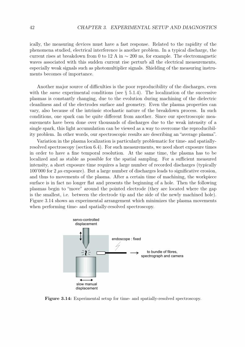
42 CHAPTER 3. EXPERIMENTAL SETUP AND DIAGNOSTICS
ically, the measuring devices must have a fast response. Related to the rapidity of thephenomena studied, electrical interference is another problem. In a typical discharge, thecurrent rises at breakdown from 0 to 12 A in ∼ 200 ns, for example. The electromagneticwaves associated with this sudden current rise perturb all the electrical measurements,especially weak signals such as photomultiplier signals. Shielding of the measuring instru-ments becomes of importance.
Another major source of difficulties is the poor reproducibility of the discharges, evenwith the same experimental conditions (see § 5.1.4). The localization of the successiveplasmas is constantly changing, due to the evolution during machining of the dielectriccleanliness and of the electrodes surface and geometry. Even the plasma properties canvary, also because of the intrinsic stochastic nature of the breakdown process. In suchconditions, one spark can be quite different from another. Since our spectroscopic mea-surements have been done over thousands of discharges due to the weak intensity of asingle spark, this light accumulation can be viewed as a way to overcome the reproducibil-ity problem. In other words, our spectroscopic results are describing an “average plasma”.
Variation in the plasma localization is particularly problematic for time- and spatially-resolved spectroscopy (section 6.4). For such measurements, we need short exposure timesin order to have a fine temporal resolution. At the same time, the plasma has to belocalized and as stable as possible for the spatial sampling. For a sufficient measuredintensity, a short exposure time requires a large number of recorded discharges (typically100’000 for 2 µs exposure). But a large number of discharges leads to significative erosion,and thus to movements of the plasma. After a certain time of machining, the workpiecesurface is in fact no longer flat and presents the beginning of a hole. Then the followingplasmas begin to “move” around the pointed electrode (they are located where the gapis the smallest, i.e. between the electrode tip and the side of the newly machined hole).Figure 3.14 shows an experimental arrangement which minimizes the plasma movementswhen performing time- and spatially-resolved spectroscopy.
endoscope : fixed
slow manualdisplacement
servo-controlleddisplacement
to bundle of fibres,spectrograph and camera
Figure 3.14: Experimental setup for time- and spatially-resolved spectroscopy.
3.6. EXPERIMENTAL DIFFICULTIES 43
The erosion is considerably reduced by using a workpiece with a large flat surface,which is manually and slowly moved horizontally. Even with a large number of sparks,the erosion is distributed over the whole surface, which remains roughly flat. The plasmamovement is thus minimized, permitting a good spatial sampling with a short exposuretime.

44 CHAPTER 3. EXPERIMENTAL SETUP AND DIAGNOSTICS
Chapter 4
Pre-breakdown of EDM discharges
The first of the four chapters presenting experimental results is dedicated to the pre-breakdown phase. The study of the mechanisms leading to breakdown is physically ofgreat interest, but it is also important from the industrial point of view. Since no materialremoval is performed during this phase, it would be interesting to understand it and tocontrol its duration, in order to reduce this “waste of time” as much as possible.
The first section of this chapter summarizes some observations made about the bubblescreated during the pre-breakdown. Current measurements are presented in the secondsection, and finally a short analysis of the pre-breakdown duration is given in the lastsection. These results are certainly not exhaustive, but they give a first insight intopre-breakdown phenomena.
4.1 BubblesDepending on the conditions, small bubbles can be generated at the electrodes as soon asthe gap voltage is applied. One can observe that:
• bubbles are created only in water, and not in oil;
• more bubbles are generated when the electric field in the gap is increased. A fewbubbles are already visible with a gap of 15 mm and 80 V, and the emission isstrongly increased by diminishing the gap distance and/or increasing the gap voltage(see § 5.1.2 for images). Note that no bubbles are generated in oil even with a gapof 100 µm and 1 kV;
• bubbles are created at the cathode;
• the contamination of the water, and consequently its conductivity, has an effect.For example, very few bubbles are generated in clean conditions (water conductivity< 3 µS/cm).
These observations suggest that the bubbles are produced by electrolysis of the water.The flow of a small electric current in the water releases gaseous hydrogen and oxygen atthe electrode surfaces, according to the following reactions:
45
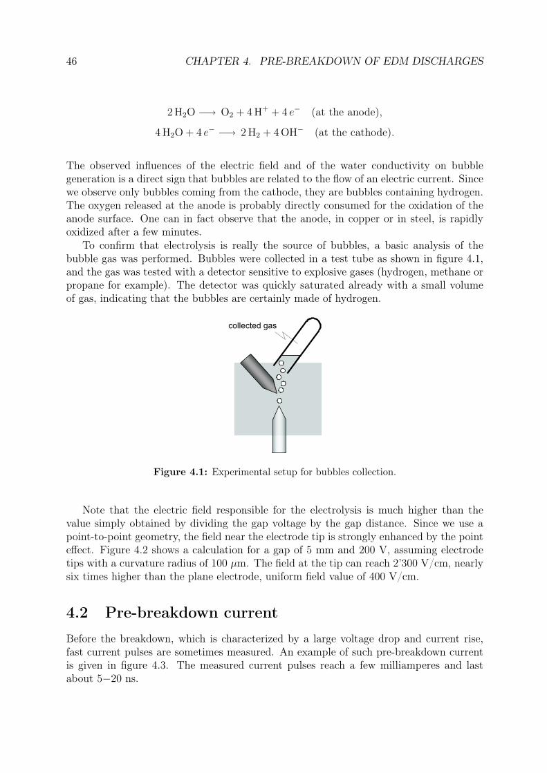
46 CHAPTER 4. PRE-BREAKDOWN OF EDM DISCHARGES
2H2O −→ O2 + 4H+ + 4 e− (at the anode),
4H2O + 4 e− −→ 2H2 + 4OH− (at the cathode).
The observed influences of the electric field and of the water conductivity on bubblegeneration is a direct sign that bubbles are related to the flow of an electric current. Sincewe observe only bubbles coming from the cathode, they are bubbles containing hydrogen.The oxygen released at the anode is probably directly consumed for the oxidation of theanode surface. One can in fact observe that the anode, in copper or in steel, is rapidlyoxidized after a few minutes.
To confirm that electrolysis is really the source of bubbles, a basic analysis of thebubble gas was performed. Bubbles were collected in a test tube as shown in figure 4.1,and the gas was tested with a detector sensitive to explosive gases (hydrogen, methane orpropane for example). The detector was quickly saturated already with a small volumeof gas, indicating that the bubbles are certainly made of hydrogen.
collected gas
Figure 4.1: Experimental setup for bubbles collection.
Note that the electric field responsible for the electrolysis is much higher than thevalue simply obtained by dividing the gap voltage by the gap distance. Since we use apoint-to-point geometry, the field near the electrode tip is strongly enhanced by the pointeffect. Figure 4.2 shows a calculation for a gap of 5 mm and 200 V, assuming electrodetips with a curvature radius of 100 µm. The field at the tip can reach 2’300 V/cm, nearlysix times higher than the plane electrode, uniform field value of 400 V/cm.
4.2 Pre-breakdown current
Before the breakdown, which is characterized by a large voltage drop and current rise,fast current pulses are sometimes measured. An example of such pre-breakdown currentis given in figure 4.3. The measured current pulses reach a few milliamperes and lastabout 5−20 ns.
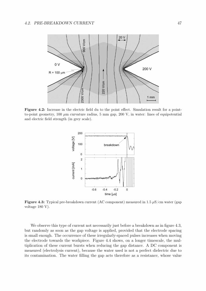
4.2. PRE-BREAKDOWN CURRENT 47
0 V
200 VR = 100 mm
20 V
220 V
/cm
2300 V
/cm
1 mm
900 V
/cm
Figure 4.2: Increase in the electric field du to the point effect. Simulation result for a point-to-point geometry, 100 µm curvature radius, 5 mm gap, 200 V, in water: lines of equipotentialand electric field strength (in grey scale).
0
100
200
0
1
2
-0.6 -0.4 -0.2 0
breakdown
time [ s]m
curr
ent [m
A]
voltage [V
]
Figure 4.3: Typical pre-breakdown current (AC component) measured in 1.5 µS/cm water (gapvoltage 180 V).
We observe this type of current not necessarily just before a breakdown as in figure 4.3,but randomly as soon as the gap voltage is applied, provided that the electrode spacingis small enough. The occurrence of these irregularly-spaced pulses increases when movingthe electrode towards the workpiece. Figure 4.4 shows, on a longer timescale, the mul-tiplication of these current bursts when reducing the gap distance. A DC component ismeasured (electrolysis current), because the water used is not a perfect dielectric due toits contamination. The water filling the gap acts therefore as a resistance, whose value
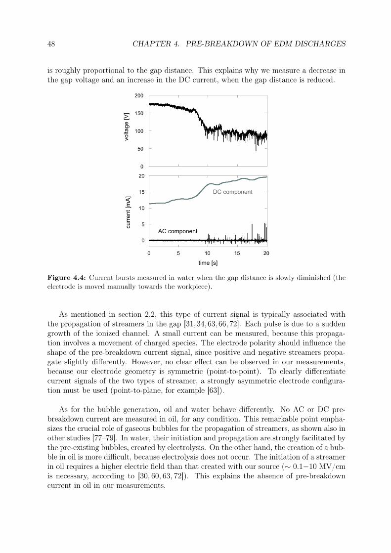
48 CHAPTER 4. PRE-BREAKDOWN OF EDM DISCHARGES
is roughly proportional to the gap distance. This explains why we measure a decrease inthe gap voltage and an increase in the DC current, when the gap distance is reduced.
0
50
100
150
200
0
5
10
15
20
0 5 10
time [s]
15 20
voltage [V
]curr
ent [m
A]
DC component
AC component
Figure 4.4: Current bursts measured in water when the gap distance is slowly diminished (theelectrode is moved manually towards the workpiece).
As mentioned in section 2.2, this type of current signal is typically associated withthe propagation of streamers in the gap [31, 34, 63, 66, 72]. Each pulse is due to a suddengrowth of the ionized channel. A small current can be measured, because this propaga-tion involves a movement of charged species. The electrode polarity should influence theshape of the pre-breakdown current signal, since positive and negative streamers propa-gate slightly differently. However, no clear effect can be observed in our measurements,because our electrode geometry is symmetric (point-to-point). To clearly differentiatecurrent signals of the two types of streamer, a strongly asymmetric electrode configura-tion must be used (point-to-plane, for example [63]).
As for the bubble generation, oil and water behave differently. No AC or DC pre-breakdown current are measured in oil, for any condition. This remarkable point empha-sizes the crucial role of gaseous bubbles for the propagation of streamers, as shown also inother studies [77–79]. In water, their initiation and propagation are strongly facilitated bythe pre-existing bubbles, created by electrolysis. On the other hand, the creation of a bub-ble in oil is more difficult, because electrolysis does not occur. The initiation of a streamerin oil requires a higher electric field than that created with our source (∼ 0.1−10 MV/cmis necessary, according to [30, 60, 63, 72]). This explains the absence of pre-breakdowncurrent in oil in our measurements.

4.2. PRE-BREAKDOWN CURRENT 49
Although the breakdown mechanisms in water and in oil should not be completelydifferent and should follow the general sequence described in section 2.2, they can nev-ertheless be influenced by different parameters. In water, the breakdown triggering iscertainly enhanced by the presence of bubbles. In oil, there are rather the contaminatingparticles that could play this role, by forming a “conductive bridge” [3,75]. Although bothbubbles and particles certainly influence the breakdown in water as in oil, the dominantcontribution is not the same in the two types of dielectric.
As expected, the conductivity of the water has an influence on pre-breakdown current[65]. Figure 4.5 presents measurements in clean water, in water contaminated with erodedparticles, and in a slightly salted solution.
200
100
0
200
100
0
200
100
0
voltage [V
]
time [ s]m
0 1 2 0 5 10 0 8 16
curr
ent [m
A]
0
10
20
30
0
10
20
30
0
10
20
30
time [ s]m time [ s]m
DC component
DC componentDCcomponent
(a) clean water
1.5 S/cmm
(b) contaminated water
7 S/cmm
(c) salted water
20 S/cmm
Figure 4.5: Effect of the water conductivity on pre-breakdown current: (a) clean water; (b) wa-ter contaminated with eroded particles; (c) salted water.
Increasing the conductivity naturally also increases the DC current. Therefore, thebubble generation by electrolysis will be more efficient and pre-breakdown currents morefrequent. This is exactly what we observe in our measurements. In clean water, the DCcurrent is almost zero and current pulses are seldom measured (typically < 1 pulse every10 µs). Then, the average number of current pulses per time unit increases with theconductivity.
The addition of external particles or other additives to the dielectric thus certainlyinfluences and facilitates the breakdown mechanism. But for a stable machining process,these additives should not increase the liquid conductivity too much. The liquid has tokeep some of its insulating properties. In the salted solution (c), short-circuits becomevery frequent. A water conductivity higher than 20 µS/cm will thus lead to an unstablesituation, prejudicial to the quality of the machining process. In real conditions of ma-chining, the dielectric is always contaminated with particles, despite continuous filtering

50 CHAPTER 4. PRE-BREAKDOWN OF EDM DISCHARGES
and cleaning of the liquid. Figure 4.5 (b) thus reflects a more realistic situation than (a)and (c).
Other studies have shown that light is emitted during the propagation of streamers.The light intensity follows the same evolution as the current [31,34,63,66,72]. An exampleof light emission measured with a photomultiplier during the pre-breakdown is given infigure 4.6.
100
120
140
0
4
8
0
0.1
0.2
0.3
-0.8 -0.6 -0.4 -0.2 0
time [ s]m
light in
tensity [arb
. unit]
curr
ent [m
A]
voltage [V
]
Figure 4.6: Light emission associated with pre-breakdown current in water (gap voltage 140 V).
Whereas the light at the breakdown is intense (saturation of the detector), the emissionassociated with streamers is very weak. Therefore, the gain of the photomultiplier has tobe set high, and this produces considerable electronic noise on the output signal. Thiskind of measurement is therefore quite difficult. Nevertheless, one can see that the lightemission is clearly correlated with the current, as expected.
4.3 Pre-breakdown duration
Once the gap voltage is applied, it takes a certain amount of time until a breakdownoccurs. This duration is not constant from a discharge to another, even if they have the

4.3. PRE-BREAKDOWN DURATION 51
same parameters. Statistics of the pre-breakdown duration have been done for differenttypes of discharges. The mean duration differs according to the discharge parameters,but the duration distribution is always of the same kind. Figure 4.7 shows histograms ofthe pre-breakdown duration measured on two types of discharges.
0 10 20 30 40 50 60 70
0
100
200
300
400
500
nu
mb
er
pre-breakdown duration [ s]m
Weibull distribution fit
0
1000
2000
3000
0 100 200 300
pre-breakdown duration [ s]m
nu
mb
er
Weibull distribution fit
(a) (b)
50 150 250
mean = 11.3 sm mean = 46.9 sm
Figure 4.7: Histograms of the pre-breakdown duration. (a) Statistics on 8’000 similar dis-charges: 6 A, 8 µs on-time, 8 µs off-time, −200 V, in water; (b) statistics on 19’000 similardischarges: 6 A, 50 µs on-time, 50 µs off-time, +200 V, in water.
The distribution of pre-breakdown duration can be well fitted with the Weibull distri-bution [118]. The probability density function of this type of distribution is
P (x|a, b) = a b xb−1 · exp(−axb) (x > 0) ,
where a and b are constant parameters. The general shape of this distribution is, startingfrom zero, an increase to a maximum value, followed by an exponential decay. The Weibulldistribution is known for describing, among others, the repartition of the pre-breakdownduration in various dielectric liquids [119,120]. The breakdown process in EDM has thusa strong stochastic nature, which clearly appears in these measurements. Although wecan optimize discharge parameters and experimental conditions to reduce the mean pre-breakdown duration (addition of electron scavengers in the dielectric for example), wewill always have distributed values. The poor reproducibility of EDM discharges canundoubtedly be related to this stochastic aspect of the breakdown.
As we will see in the next chapter, the stochastic nature of the breakdown has apractical consequence for plasma imaging. Since it is impossible to predict precisely whenthe next breakdown will occur, the camera opening for the exposure of a given dischargecan only be triggered with the beginning of this very discharge. We cannot anticipate thebeginning of the next discharge, as could be done with pulsed RF plasmas, for example.

52 CHAPTER 4. PRE-BREAKDOWN OF EDM DISCHARGES

Chapter 5
Imaging diagnostics of EDM discharges
The first section of this chapter presents images taken from films that were recordedduring the EDM machining process. Images of the plasma itself are analyzed in thesecond section. Finally, the third and fourth sections are respectively dedicated to imagesof the plasma at the beginning and at the end of the discharge.
5.1 Imaging of the EDM process
5.1.1 Erosion
Figure 5.1 shows a typical example of what can be observed during machining.
1 2 3 4
5 6 7 8
1 mm
electrode
workpiece spark
bubbles
eroded cavity
Figure 5.1: Images taken during the machining process (1 ms exposure; Cu electrode, steelworkpiece, 8 A, 50 µs on-time, + 200 V, water). Sparks and bubbles are clearly visible. Theduration of the whole sequence is approximatively 40 s.
53

54 CHAPTER 5. IMAGING DIAGNOSTICS OF EDM DISCHARGES
The workpiece surface, completely flat on image 1 before machining, is slightly erodedby the successive sparks. After a few tens of seconds of machining, i.e. after a fewhundreds of thousands of sparks, a small cavity is formed (image 8). Some of these sparksare visible on images 2, 4, 5 and 7. The heat released by the discharges generates vaporbubbles close to the electrode gap. They can be clearly seen on images 3, 6 and 7 forexample.
5.1.2 Bubbles
Different types of bubbles can be observed. As mentioned in section 4.1, hydrogen bubblesare released during pre-breakdown in water by electrolysis. During machining, the heatof the plasma is generating vapor bubbles, in water as in oil. Images of these differentkinds of bubbles are given in figure 5.2.
(a) H bubbles duringin water
2pre-breakdown
(b) vapor bubbles duringerosion in water
(c) vapor bubbles duringerosion in oil
1 mm 1 mm
electrode
1 mm
electrode
Figure 5.2: Different types of bubbles generated during the EDM process: (a) small hydrogenbubbles created by electrolysis during pre-breakdown in water (large and small gap, + 200 V);(b) water vapor bubbles thermally induced during machining (8 A, 50 µs); (c) oil vapor bubblesthermally induced during machining (6 A, 6 µs).
By zooming on the images of figure 5.2 (a), the diameter of the electrolysis bubbles canbe roughly estimated around 30 − 100 µm. The generation of these hydrogen bubbles isstrongly enhanced with an increase in the electric field. With a small gap (bottom imageof figure 5.2 (a)), one can in fact observe numerous bubbles ejected from the gap withhigh velocity, leading even to turbulent phenomena (vortices).
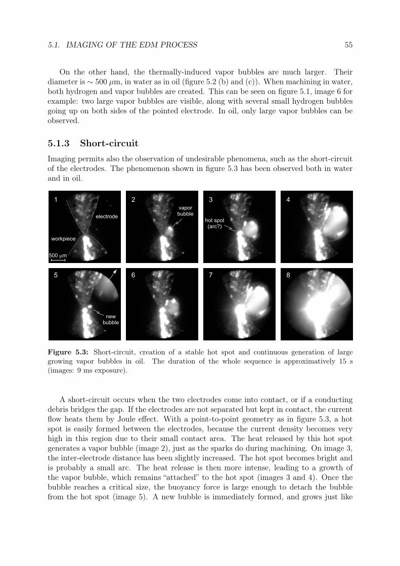
5.1. IMAGING OF THE EDM PROCESS 55
On the other hand, the thermally-induced vapor bubbles are much larger. Theirdiameter is ∼ 500 µm, in water as in oil (figure 5.2 (b) and (c)). When machining in water,both hydrogen and vapor bubbles are created. This can be seen on figure 5.1, image 6 forexample: two large vapor bubbles are visible, along with several small hydrogen bubblesgoing up on both sides of the pointed electrode. In oil, only large vapor bubbles can beobserved.
5.1.3 Short-circuit
Imaging permits also the observation of undesirable phenomena, such as the short-circuitof the electrodes. The phenomenon shown in figure 5.3 has been observed both in waterand in oil.
1 2 3 4
5 6 7 8
hot spot(arc?)
vaporbubble
newbubble
electrode
workpiece
500 mm
Figure 5.3: Short-circuit, creation of a stable hot spot and continuous generation of largegrowing vapor bubbles in oil. The duration of the whole sequence is approximatively 15 s(images: 9 ms exposure).
A short-circuit occurs when the two electrodes come into contact, or if a conductingdebris bridges the gap. If the electrodes are not separated but kept in contact, the currentflow heats them by Joule effect. With a point-to-point geometry as in figure 5.3, a hotspot is easily formed between the electrodes, because the current density becomes veryhigh in this region due to their small contact area. The heat released by this hot spotgenerates a vapor bubble (image 2), just as the sparks do during machining. On image 3,the inter-electrode distance has been slightly increased. The hot spot becomes bright andis probably a small arc. The heat release is then more intense, leading to a growth ofthe vapor bubble, which remains “attached” to the hot spot (images 3 and 4). Once thebubble reaches a critical size, the buoyancy force is large enough to detach the bubblefrom the hot spot (image 5). A new bubble is immediately formed, and grows just like
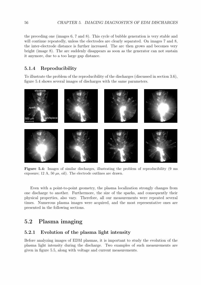
56 CHAPTER 5. IMAGING DIAGNOSTICS OF EDM DISCHARGES
the preceding one (images 6, 7 and 8). This cycle of bubble generation is very stable andwill continue repeatedly, unless the electrodes are clearly separated. On images 7 and 8,the inter-electrode distance is further increased. The arc then grows and becomes verybright (image 8). The arc suddenly disappears as soon as the generator can not sustainit anymore, due to a too large gap distance.
5.1.4 Reproducibility
To illustrate the problem of the reproducibility of the discharges (discussed in section 3.6),figure 5.4 shows several images of discharges with the same parameters.
electrode
workpiece
spark
500 mm
Figure 5.4: Images of similar discharges, illustrating the problem of reproducibility (9 msexposure; 12 A, 50 µs, oil). The electrode outlines are drawn.
Even with a point-to-point geometry, the plasma localization strongly changes fromone discharge to another. Furthermore, the size of the sparks, and consequently theirphysical properties, also vary. Therefore, all our measurements were repeated severaltimes. Numerous plasma images were acquired, and the most representative ones arepresented in the following sections.
5.2 Plasma imaging
5.2.1 Evolution of the plasma light intensity
Before analyzing images of EDM plasmas, it is important to study the evolution of theplasma light intensity during the discharge. Two examples of such measurements aregiven in figure 5.5, along with voltage and current measurements.

5.2. PLASMA IMAGING 57
0
2
4
6
0 2 4 6 8
0
20
40
60
80
100
time [ s]m
curr
ent [A
]lig
ht in
tensity [arb
. un
it]
volta
ge [V
]
0
0.4
0.8
1.2
(a) short discharge (b) long discharge
0
4
8
0
100
200
0
0.8
1.6
0 20 40 60 80 100
time [ s]m
0.4
1.2
2
6
50
150
Figure 5.5: Evolution of the plasma light intensity, of the current and of the voltage during asingle discharge: (a) short discharge (4 A, 8 µs, water); (b) long discharge (8 A, 100 µs, water).
Two phases can be distinguished: the breakdown phase and the discharge phase. Themajor part of the light is emitted during the breakdown phase, i.e. approximately duringthe first 500 ns after the breakdown (see figure 5.5 (a)). During the discharge itself,the light emission is 10 to 150 times less intense. In figure 5.5 (b), the first light peakseems to last much longer than 500 ns. This is an artefact due to the saturation of thephotomultiplier. For this measurement, the gain of the detector has in fact been set higherin order to better visualize the light emission during the discharge phase. The intensityof the first peak is thus in reality much higher and lasts less than 1 µs.
The light emission during the discharge phase becomes much more intense when in-creasing the discharge current. Furthermore, the oscillations observed on light intensitymeasurements in figure 5.5 (b) are correlated to those on current (the current waveformis caused by the regulation system of the generator). This shows that these two physicalvalues are unsurprisingly interdependent.
From the erosion point of view, the first microsecond seems to be very different fromthe rest of the discharge. The high intensity of the first light peak suggests that a massiveflow of energy is brought to the workpiece during the breakdown phase. Due to the shortduration of this event (< 1 µs), it is probable that only the workpiece surface is affected bythis primary energy flow, while the workpiece bulk remains unaffected. A burst of energywill in fact directly evaporate only the very superficial layers of the workpiece. The bulk isnot affected, because it can not absorb this high amount of energy by conduction on such
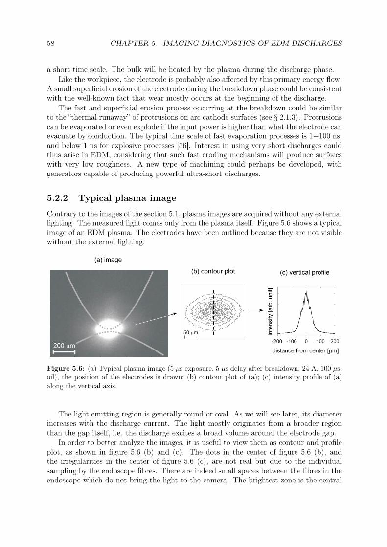
58 CHAPTER 5. IMAGING DIAGNOSTICS OF EDM DISCHARGES
a short time scale. The bulk will be heated by the plasma during the discharge phase.Like the workpiece, the electrode is probably also affected by this primary energy flow.
A small superficial erosion of the electrode during the breakdown phase could be consistentwith the well-known fact that wear mostly occurs at the beginning of the discharge.
The fast and superficial erosion process occurring at the breakdown could be similarto the “thermal runaway” of protrusions on arc cathode surfaces (see § 2.1.3). Protrusionscan be evaporated or even explode if the input power is higher than what the electrode canevacuate by conduction. The typical time scale of fast evaporation processes is 1−100 ns,and below 1 ns for explosive processes [56]. Interest in using very short discharges couldthus arise in EDM, considering that such fast eroding mechanisms will produce surfaceswith very low roughness. A new type of machining could perhaps be developed, withgenerators capable of producing powerful ultra-short discharges.
5.2.2 Typical plasma image
Contrary to the images of the section 5.1, plasma images are acquired without any externallighting. The measured light comes only from the plasma itself. Figure 5.6 shows a typicalimage of an EDM plasma. The electrodes have been outlined because they are not visiblewithout the external lighting.
200 mm
50 mm
(a) image
(b) contour plot (c) vertical profile
-200 -100 0 100 200
distance from center [ m]m
inte
nsity [arb
. unit]
Figure 5.6: (a) Typical plasma image (5 µs exposure, 5 µs delay after breakdown; 24 A, 100 µs,oil), the position of the electrodes is drawn; (b) contour plot of (a); (c) intensity profile of (a)along the vertical axis.
The light emitting region is generally round or oval. As we will see later, its diameterincreases with the discharge current. The light mostly originates from a broader regionthan the gap itself, i.e. the discharge excites a broad volume around the electrode gap.
In order to better analyze the images, it is useful to view them as contour and profileplot, as shown in figure 5.6 (b) and (c). The dots in the center of figure 5.6 (b), andthe irregularities in the center of figure 5.6 (c), are not real but due to the individualsampling by the endoscope fibres. There are indeed small spaces between the fibres in theendoscope which do not bring the light to the camera. The brightest zone is the central
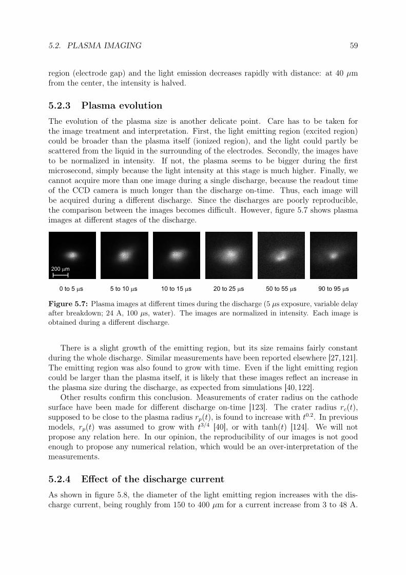
5.2. PLASMA IMAGING 59
region (electrode gap) and the light emission decreases rapidly with distance: at 40 µmfrom the center, the intensity is halved.
5.2.3 Plasma evolution
The evolution of the plasma size is another delicate point. Care has to be taken forthe image treatment and interpretation. First, the light emitting region (excited region)could be broader than the plasma itself (ionized region), and the light could partly bescattered from the liquid in the surrounding of the electrodes. Secondly, the images haveto be normalized in intensity. If not, the plasma seems to be bigger during the firstmicrosecond, simply because the light intensity at this stage is much higher. Finally, wecannot acquire more than one image during a single discharge, because the readout timeof the CCD camera is much longer than the discharge on-time. Thus, each image willbe acquired during a different discharge. Since the discharges are poorly reproducible,the comparison between the images becomes difficult. However, figure 5.7 shows plasmaimages at different stages of the discharge.
0 to 5 sm 5 to 10 sm 10 to 15 sm 20 to 25 sm 50 to 55 sm 90 to 95 sm
200 mm
Figure 5.7: Plasma images at different times during the discharge (5 µs exposure, variable delayafter breakdown; 24 A, 100 µs, water). The images are normalized in intensity. Each image isobtained during a different discharge.
There is a slight growth of the emitting region, but its size remains fairly constantduring the whole discharge. Similar measurements have been reported elsewhere [27,121].The emitting region was also found to grow with time. Even if the light emitting regioncould be larger than the plasma itself, it is likely that these images reflect an increase inthe plasma size during the discharge, as expected from simulations [40,122].
Other results confirm this conclusion. Measurements of crater radius on the cathodesurface have been made for different discharge on-time [123]. The crater radius rc(t),supposed to be close to the plasma radius rp(t), is found to increase with t0.2. In previousmodels, rp(t) was assumed to grow with t3/4 [40], or with tanh(t) [124]. We will notpropose any relation here. In our opinion, the reproducibility of our images is not goodenough to propose any numerical relation, which would be an over-interpretation of themeasurements.
5.2.4 Effect of the discharge current
As shown in figure 5.8, the diameter of the light emitting region increases with the dis-charge current, being roughly from 150 to 400 µm for a current increase from 3 to 48 A.
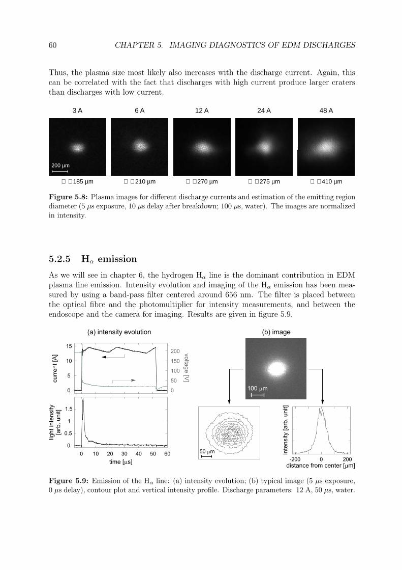
60 CHAPTER 5. IMAGING DIAGNOSTICS OF EDM DISCHARGES
Thus, the plasma size most likely also increases with the discharge current. Again, thiscan be correlated with the fact that discharges with high current produce larger cratersthan discharges with low current.
3 A 6 A 12 A 24 A 48 A
200 mµ
∅ ≅ 185 mµ ∅ ≅ 210 mµ ∅ ≅ 270 mµ ∅ ≅ 275 mµ ∅ ≅ 410 mµ
Figure 5.8: Plasma images for different discharge currents and estimation of the emitting regiondiameter (5 µs exposure, 10 µs delay after breakdown; 100 µs, water). The images are normalizedin intensity.
5.2.5 Hα emission
As we will see in chapter 6, the hydrogen Hα line is the dominant contribution in EDMplasma line emission. Intensity evolution and imaging of the Hα emission has been mea-sured by using a band-pass filter centered around 656 nm. The filter is placed betweenthe optical fibre and the photomultiplier for intensity measurements, and between theendoscope and the camera for imaging. Results are given in figure 5.9.
time [ s]m
curr
ent [A
]lig
ht in
tensity
[arb
. unit]
volta
ge [V
]
(a) intensity evolution (b) image
0
100
200
0
5
10
15
0
0.5
1
1.5
0 20 40 60
100 mm
50 mm
-200 0 200distance from center [ m]m
inte
nsity [arb
. unit]
10 30 50
150
50
Figure 5.9: Emission of the Hα line: (a) intensity evolution; (b) typical image (5 µs exposure,0 µs delay), contour plot and vertical intensity profile. Discharge parameters: 12 A, 50 µs, water.

5.3. BEGINNING OF THE DISCHARGE : FAST IMAGING 61
The intensity evolution of this line is similar to the evolution of the total emission,given previously in figure 5.5. The major part of the light is emitted during the breakdownphase. Similarly, the images obtained with the Hα filter are very similar to those obtainedwithout it (see figure 5.6). The emitting region has the same shape, size and intensityprofiles. We can thus conclude that the Hα line is emitted by the whole plasma volume.
5.3 Beginning of the discharge : Fast imagingFigure 5.10 shows fast imaging of the first 300 ns of the discharge, obtained with the ICCDcamera. This time interval corresponds to the emission of the first light peak and to thefirst fast current rise (see figure 5.5 (a)). This interval is thus important in the plasmaevolution: it is during the very beginning of the discharge that the plasma is forming andthat a high amount of energy is brought into it.
50 to 100 ns
100 to 150 ns
150 to 200 ns
200 to 250 ns
250 to 300 ns
time [ s]m
0 0.5 1
0
0.5
1
0
0.5
1
0
0.5
1
0
0.5
1
0
0.5
1
exposure
V/200 [V]I/8 [A]
Figure 5.10: Fast imaging of the discharge beginning along with current and voltage evolution(50 ns exposure, variable delay; 6 A, water). The images are normalized in intensity. Each imageis obtained during a different discharge.
The exposure time is 50 ns for each image, with variable delays. There is always a 50 nsintrinsic delay between the trigger signal (current rise at the breakdown) and the cameraopening, due to gating electronics and cables. Since we cannot anticipate the breakdown

62 CHAPTER 5. IMAGING DIAGNOSTICS OF EDM DISCHARGES
for the camera triggering as previously mentioned in section 4.3, the first image can onlybe acquired 50 ns after the breakdown.
Between 100 and 200 ns after the breakdown, the current reaches its maximum. Thelight intensity is also at its maximum. However, on the plasma images, no clear evolution isvisible from 50 to 300 ns: size and geometry remain constant. Images obtained with delayslonger than 300 ns are not shown here, but they are similar to those of the figure 5.10.This shows that the plasma develops very rapidly (within 50 ns) after the breakdown,and then remains quite stable.
5.4 End of the discharge and post-discharge
Since the major part of the workpiece material is removed at the end of the dischargewhen the plasma collapses, the transition from the discharge to the post-discharge isparticularly interesting to study. This stage in the EDM process is certainly crucial forthe optimization of the material removal rate.
The evolution of the light intensity at the transition and during the post-discharge ispresented in figure 5.11.
0
150 250 350 450
time [ s]m
2
4
6
8
0
50
100
150
200
volta
ge [V
]in
tensity [arb
. unit]
50
0
1.4
0.7
curr
ent [A
]
post-discharge light
discharge light
Figure 5.11: Evolution of the light intensity during a post-discharge (discharge: 6 A, 50 µs,water).
As soon as the current is shut down, it drops rapidly to zero, and the light intensity issimultaneously also dropping fast. But there is still a weak slowly-decaying light emission,typically until 300 µs after the end of the discharge. The corresponding images of thetransition are given in figure 5.12.
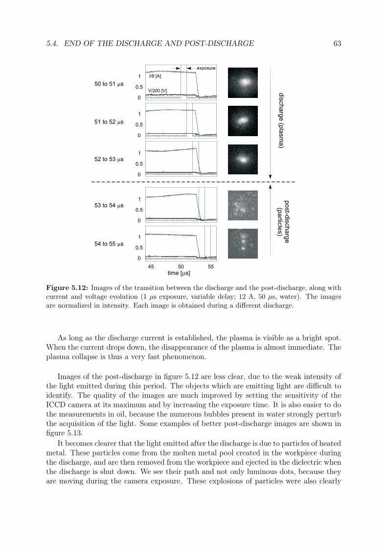
5.4. END OF THE DISCHARGE AND POST-DISCHARGE 63
time [ s]m
45 50
0
0.5
1
exposure
V/200 [V]
I/8 [A]
55
0
0.5
1
0
0.5
1
0
0.5
1
0
0.5
1
dis
charg
e (p
lasm
a)
post-d
ischarg
e(p
artic
les)
50 to 51 sm
51 to 52 sm
52 to 53 sm
53 to 54 sm
54 to 55 sm
Figure 5.12: Images of the transition between the discharge and the post-discharge, along withcurrent and voltage evolution (1 µs exposure, variable delay; 12 A, 50 µs, water). The imagesare normalized in intensity. Each image is obtained during a different discharge.
As long as the discharge current is established, the plasma is visible as a bright spot.When the current drops down, the disappearance of the plasma is almost immediate. Theplasma collapse is thus a very fast phenomenon.
Images of the post-discharge in figure 5.12 are less clear, due to the weak intensity ofthe light emitted during this period. The objects which are emitting light are difficult toidentify. The quality of the images are much improved by setting the sensitivity of theICCD camera at its maximum and by increasing the exposure time. It is also easier to dothe measurements in oil, because the numerous bubbles present in water strongly perturbthe acquisition of the light. Some examples of better post-discharge images are shown infigure 5.13.
It becomes clearer that the light emitted after the discharge is due to particles of heatedmetal. These particles come from the molten metal pool created in the workpiece duringthe discharge, and are then removed from the workpiece and ejected in the dielectric whenthe discharge is shut down. We see their path and not only luminous dots, because theyare moving during the camera exposure. These explosions of particles were also clearly

64 CHAPTER 5. IMAGING DIAGNOSTICS OF EDM DISCHARGES
200 mm
Figure 5.13: Incandescence of the removed particles after a discharge. Each image is takenduring a single post-discharge (100 µs exposure; 12 A, 50 µs, oil).
visible on figure 5.4. However, on these previous images, the exposure time was longenough to record both the spark and the post-discharge. Therefore, the interpretationof these luminous paths was not obvious. They could have been attributed to bubblesfor example, which would scatter the light of the spark. On the other hand, images offigure 5.13 are time-resolved and the light is acquired only during post-discharges. Theinterpretation is thus less ambiguous.
In order to confirm the hypothesis of the metal particles, optical emission spectroscopyof the post-discharge light has been performed. An example of the spectrum is shown infigure 5.14.
400 500 600 700 800
wavelength [nm]
inte
nsity [arb
. unit] blackbody fit
2300 K
Figure 5.14: Optical emission spectrum of the post-discharge light, with a 2’300 K blackbodyfit. The light measurement is time integrated over thousands of post-discharges (50 µs exposure,150 g/mm grating; 16 A, 50 µs, oil).
Spectroscopy shows that the post-discharge light emission is close to a blackbodyradiation, which confirms that the emitters are hot metal particles. The spectrum infigure 5.14 is quite noisy, due to the low intensity of the light emission. Fitting severalpost-discharge spectra with Planck’s law, the temperature of the emitters is found to bearound 2’200 K (± 100 K). Since the melting point of steel is ∼ 1’700 K, the particles arestill in a liquid state in the very beginning of the post-discharge. The temperature found
5.4. END OF THE DISCHARGE AND POST-DISCHARGE 65
is consistent with metallurgical analyses of the modified layers of the workpiece [25,125].In these studies, the maximum temperature of the workpiece surface reached during theEDM process has been estimated to be around 3’000 K.
The particle size can be measured on the images. We found that the largest particleshave a diameter of ∼ 30 µm, which is in good agreement with previous work on spark-eroded particles [126, 127]. The particle speed can also be estimated from images. Themaximum speed is around 3 m/s. Since the particles move in the liquid, their trajectoriesand speed can be affected if a liquid flow velocity is imposed.

66 CHAPTER 5. IMAGING DIAGNOSTICS OF EDM DISCHARGES
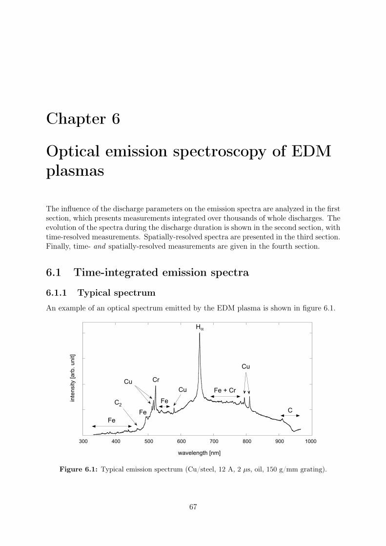
Chapter 6
Optical emission spectroscopy of EDMplasmas
The influence of the discharge parameters on the emission spectra are analyzed in the firstsection, which presents measurements integrated over thousands of whole discharges. Theevolution of the spectra during the discharge duration is shown in the second section, withtime-resolved measurements. Spatially-resolved spectra are presented in the third section.Finally, time- and spatially-resolved measurements are given in the fourth section.
6.1 Time-integrated emission spectra
6.1.1 Typical spectrum
An example of an optical spectrum emitted by the EDM plasma is shown in figure 6.1.
300 400 500 600 700 800 900 1000
Ha
C
Cu
C2
Fe
Cr
Cu
Cu
Fe
Fe
Fe + Cr
wavelength [nm]
inte
nsity [arb
. unit]
Figure 6.1: Typical emission spectrum (Cu/steel, 12 A, 2 µs, oil, 150 g/mm grating).
67

68 CHAPTER 6. OPTICAL EMISSION SPECTROSCOPY OF EDM PLASMAS
The dominant line is the Balmer Hα line emitted by atomic hydrogen, which comesfrom the cracking of the dielectric molecules. Some lines of atomic carbon and C2
molecules (Swan system) are also visible. This indicates that the organic molecules ofoil are almost completely cracked by the discharge. As previously mentioned in § 5.2.5,imaging showed that the Hα line is emitted by the whole plasma volume. This can beunderstood considering the fact that the plasma is formed by cracking and ionizing the di-electric molecules and atoms. Since the hydrogen source is the dielectric, hydrogen atomsare present everywhere in the plasma. Although the Hα line is dominant, the remainingBalmer series lines such as Hβ (486.13 nm) or Hγ (434.05 nm) are not observed. Thisremarkable point will be discussed later, in section 7.2.
The plasma is contaminated by impurities: several lines of atomic copper from theelectrode are present, along with many lines originating from atomic iron, chromium andcarbon of the removed material of the steel workpiece. These lines can be seen in moredetail in figure 6.2.
360 380 400 420 440
460 480 500 520 540 560 900 920 940 960
wavelength [nm]
inte
nsity [arb
. unit]
wavelength [nm]
wavelength [nm]
inte
nsity [arb
. unit]
CC C
C
C
CC
Cr
FeC2
FeFe
Fe
Fe
Fe
Fe
Cu
CuCu
Cr
Fe
C2
Fe
C2
CrFeFe
Cr
Cr
Fe
C2
Fe Fe FeFe
Fe
Fe
Fe
Fe
Fe
FeFe
Fe
Fe
Fe
Fe
Fe
FeFe
Fe
Fe FeFe
Fe
FeFe
Fe
Fe
Figure 6.2: Typical emission spectrum, details (Cu/steel, 12 A, 100 µs, oil, 600 g/mm grating).
The fact that all observed lines are atomic lines (along with a few neutral molecularlines) and that no ionic lines are visible, is a first indication that the plasma is cold. Theexcitation of ions requires indeed higher energy than the excitation of atoms. Furthermore,

6.1. TIME-INTEGRATED EMISSION SPECTRA 69
atoms and ions of metallic elements are easily excited, more easily than those of non-metallic elements. For example, the excited state energies of visible transitions of Fe atomsand of Fe+ ions are respectively around 3 and 11 eV (from the ground state of atoms andions respectively), but for C atoms and for C+ ions they are respectively around 8 and22 eV [128, 129]. Thus, the absence of ionic lines of iron, copper or chromium indicatesclearly that the plasma temperature is low. Since sparks in gases are known to be highlyionized plasmas [49], EDM sparks should nevertheless also be fairly ionized.
The low excitation energy of metallic atoms explains the abundance and the relativelyhigh intensity of their lines in the EDM plasma emission (see for example the numerousFe lines in figure 6.2). It should be noted that this abundance does not mean that alarge amount of metal is present in the plasma. In electric arcs for example, the lightemission is dominated by metallic lines already with a contamination of a few percents ofmetal. It is also well known that metallic impurities strongly cool down fusion plasmasin tokamaks, because of their strong radiation. Thus, a quantitative estimation of themetallic contamination in the EDM plasma from our spectra would be hazardous.
An intense broadband continuum radiation is also observed. The origin of this radia-tion remains unclear. Blackbody fits do not match well with our measurements. Thus, acontinuous emission by heated electrodes or metal particles is unlikely. It is more probablethat this continuum is due to free-bound transitions, i.e. radiation emitted during recom-bination processes. Free-free radiation is also another plausible source. Since moleculesgenerally emit a broadband spectrum, molecules or fragments of molecules from the di-electric certainly also participate to the continuum [34,63].
6.1.2 Effect of the dielectric
Figure 6.3 shows emission spectra obtained in different dielectrics.
400 600 800
(a) water (b) oil (c) liquid nitrogen
inte
nsi
ty [arb
. unit]
600 800 1000500 700 900
wavelength [nm] wavelength [nm] wavelength [nm]
500 700 900 400 600 800500 700 900
CuCu
O
O
Cu
Ha H
a
CuCu
CuC
C2
Cu
Cu
Cu
N
N
NN
N
Figure 6.3: Effect of the dielectric on the emission spectrum (Cu/steel, 150 g/mm grating):(a) water, 12 A, 2 µs; (b) oil, 12 A, 2 µs; (c) liquid nitrogen, 48 A, 2 µs.
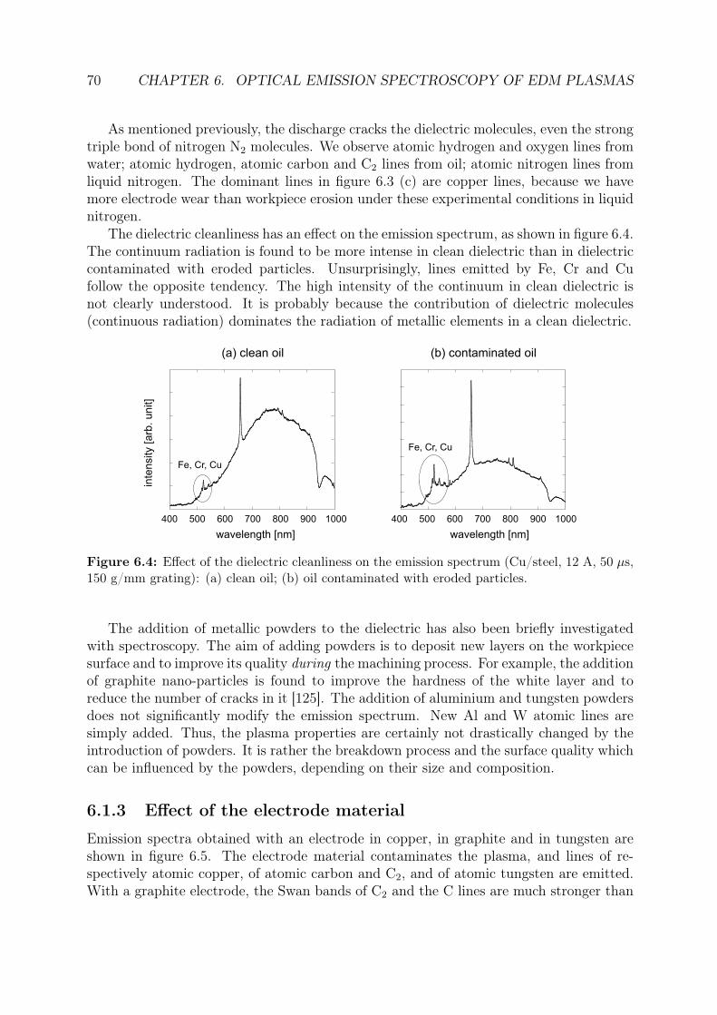
70 CHAPTER 6. OPTICAL EMISSION SPECTROSCOPY OF EDM PLASMAS
As mentioned previously, the discharge cracks the dielectric molecules, even the strongtriple bond of nitrogen N2 molecules. We observe atomic hydrogen and oxygen lines fromwater; atomic hydrogen, atomic carbon and C2 lines from oil; atomic nitrogen lines fromliquid nitrogen. The dominant lines in figure 6.3 (c) are copper lines, because we havemore electrode wear than workpiece erosion under these experimental conditions in liquidnitrogen.
The dielectric cleanliness has an effect on the emission spectrum, as shown in figure 6.4.The continuum radiation is found to be more intense in clean dielectric than in dielectriccontaminated with eroded particles. Unsurprisingly, lines emitted by Fe, Cr and Cufollow the opposite tendency. The high intensity of the continuum in clean dielectric isnot clearly understood. It is probably because the contribution of dielectric molecules(continuous radiation) dominates the radiation of metallic elements in a clean dielectric.
400 600 800
(a) clean oil (b) contaminated oil
inte
nsity [arb
. unit]
wavelength [nm] wavelength [nm]
500 700 900 1000 400 600 800500 700 900 1000
Fe, Cr, Cu
Fe, Cr, Cu
Figure 6.4: Effect of the dielectric cleanliness on the emission spectrum (Cu/steel, 12 A, 50 µs,150 g/mm grating): (a) clean oil; (b) oil contaminated with eroded particles.
The addition of metallic powders to the dielectric has also been briefly investigatedwith spectroscopy. The aim of adding powders is to deposit new layers on the workpiecesurface and to improve its quality during the machining process. For example, the additionof graphite nano-particles is found to improve the hardness of the white layer and toreduce the number of cracks in it [125]. The addition of aluminium and tungsten powdersdoes not significantly modify the emission spectrum. New Al and W atomic lines aresimply added. Thus, the plasma properties are certainly not drastically changed by theintroduction of powders. It is rather the breakdown process and the surface quality whichcan be influenced by the powders, depending on their size and composition.
6.1.3 Effect of the electrode material
Emission spectra obtained with an electrode in copper, in graphite and in tungsten areshown in figure 6.5. The electrode material contaminates the plasma, and lines of re-spectively atomic copper, of atomic carbon and C2, and of atomic tungsten are emitted.With a graphite electrode, the Swan bands of C2 and the C lines are much stronger than

6.1. TIME-INTEGRATED EMISSION SPECTRA 71
in figure 6.1 for example, because the carbon contamination of the plasma due to thegraphite electrode is much greater than the carbon produced by the cracking of the oil.The tungsten lines are very difficult to observe because they are located in the samespectral region as many iron lines, which are more intense.
(a) copper (b) graphite (c) tungsten
400 600 800
inte
nsi
ty [arb
. unit]
wavelength [nm]
500 700 900 400 600 800
wavelength [nm]
500 700 900 400 600 800
wavelength [nm]
500 700 900
CuCu
Cu
C
C2
W
C
Figure 6.5: Effect of the electrode material on the emission spectrum (12 A, 5 µs, oil, 150 g/mmgrating): (a) Cu/steel; (b) graphite/steel; (c) W/steel.
The use of a zinc electrode produces a spectrum quite different from the others, asshown in figure 6.6. It should be noted that zinc is never used as electrode material indie-sinking machines, but only as a coating layer of the wire in wire-cutting machines.
inte
nsity [arb
. unit]
wavelength [nm]
300 400 500 600 700 800 900 1000
Ha
Zn
Zn
Zn
Zn+
Zn+
Zn+
Zn+
C
Figure 6.6: Emission spectrum with a zinc electrode (Zn/steel, 12 A, 12 µs, −200 V, oil,150 g/mm grating).
In addition to the Hα line and C lines, both atomic Zn lines and ionic Zn+ linesare emitted, with high intensities. Zinc is the only material tested in this work thatproduces ionic lines. The wavelengths of these lines, along with those of all other main
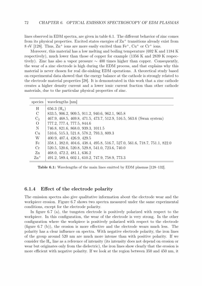
72 CHAPTER 6. OPTICAL EMISSION SPECTROSCOPY OF EDM PLASMAS
lines observed in EDM spectra, are given in table 6.1. The different behavior of zinc comesfrom its physical properties. Excited states energies of Zn+ transitions already exist from8 eV [128]. Thus, Zn+ ions are more easily excited than Fe+, Cu+ or Cr+ ions.
Moreover, this material has a low melting and boiling temperature (692 K and 1184 Krespectively), much lower than those of copper for example (1356 K and 2839 K respec-tively). Zinc has also a vapor pressure ∼ 400 times higher than copper. Consequently,the wear of a zinc electrode is high during the EDM process, and that explains why thismaterial is never chosen for real die-sinking EDM operations. A theoretical study basedon experimental data showed that the energy balance at the cathode is strongly related tothe electrode material properties [28]. It is demonstrated in this work that a zinc cathodecreates a higher density current and a lower ionic current fraction than other cathodematerials, due to the particular physical properties of zinc.
species wavelengths [nm]
H 656.3 (Hα)C 833.5, 906.2, 909.5, 911.2, 940.6, 962.1, 965.8C2 467.9, 468.5, 469.8, 471.5, 473.7, 512.9, 516.5, 563.6 (Swan system)O 777.2, 777.4, 777.5, 844.6N 746.8, 821.6, 868.0, 939.3, 1011.5Cu 510.6, 515.3, 521.8, 578.2, 793.3, 809.3W 400.9, 407.4, 426.9, 429.5Fe 358.1, 382.0, 404.6, 438.4, 495.8, 516.7, 527.0, 561.6, 718.7, 751.1, 822.0Cr 520.5, 520.6, 520.8, 529.8, 541.0, 723.6, 740.0Zn 468.0, 472.2, 481.1, 636.2Zn+ 491.2, 589.4, 602.1, 610.2, 747.9, 758.9, 773.3
Table 6.1: Wavelengths of the main lines emitted by EDM plasmas [128–132].
6.1.4 Effect of the electrode polarity
The emission spectra also give qualitative information about the electrode wear and theworkpiece erosion. Figure 6.7 shows two spectra measured under the same experimentalconditions, except for the electrode polarity.
In figure 6.7 (a), the tungsten electrode is positively polarized with respect to theworkpiece. In this configuration, the wear of the electrode is very strong. In the otherconfiguration where the workpiece is positively polarized with respect to the electrode(figure 6.7 (b)), the erosion is more effective and the electrode wears much less. Thepolarity has a clear influence on spectra. With negative electrode polarity, the iron linesof the group around 520 nm are much more intense than with positive polarity. If weconsider the Hα line as a reference of intensity (its intensity does not depend on erosion orwear but originates only from the dielectric), the iron lines show clearly that the erosion ismore efficient with negative polarity. If we look at the region between 350 and 450 nm, it
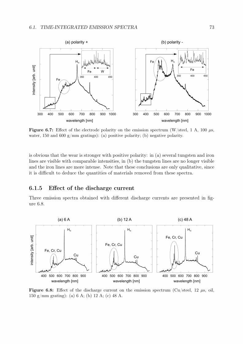
6.1. TIME-INTEGRATED EMISSION SPECTRA 73
(b) polarity -(a) polarity +
inte
nsity [arb
. unit]
wavelength [nm]
300 400 500 600 700 800 900 1000
wavelength [nm]
300 400 500 600 700 800 900 1000
350 400 450
FeFe
W
Fe
FeHa
Ha
350 400 450
Figure 6.7: Effect of the electrode polarity on the emission spectrum (W/steel, 1 A, 100 µs,water, 150 and 600 g/mm gratings): (a) positive polarity; (b) negative polarity.
is obvious that the wear is stronger with positive polarity: in (a) several tungsten and ironlines are visible with comparable intensities, in (b) the tungsten lines are no longer visibleand the iron lines are more intense. Note that these conclusions are only qualitative, sinceit is difficult to deduce the quantities of materials removed from these spectra.
6.1.5 Effect of the discharge current
Three emission spectra obtained with different discharge currents are presented in fig-ure 6.8.
400 600 800
(a) 6 A (b) 12 A (c) 48 A
inte
nsity [arb
. unit]
wavelength [nm] wavelength [nm]
500 700 900 400 600 800500 700 900
wavelength [nm]
400 600 800500 700 900
Ha
Ha
Ha
Fe, Cr, Cu
Fe, Cr, Cu
Fe, Cr, Cu
CuCu
Cu
Figure 6.8: Effect of the discharge current on the emission spectrum (Cu/steel, 12 µs, oil,150 g/mm grating): (a) 6 A; (b) 12 A; (c) 48 A.
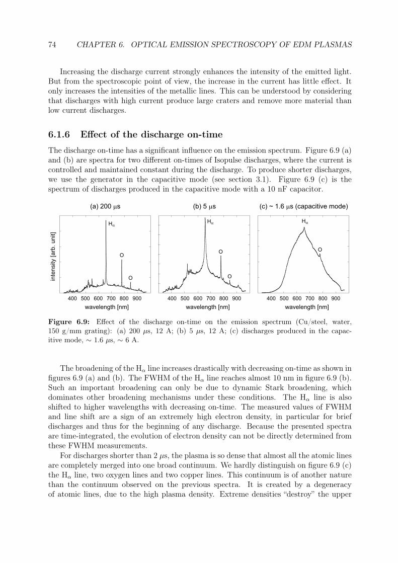
74 CHAPTER 6. OPTICAL EMISSION SPECTROSCOPY OF EDM PLASMAS
Increasing the discharge current strongly enhances the intensity of the emitted light.But from the spectroscopic point of view, the increase in the current has little effect. Itonly increases the intensities of the metallic lines. This can be understood by consideringthat discharges with high current produce large craters and remove more material thanlow current discharges.
6.1.6 Effect of the discharge on-time
The discharge on-time has a significant influence on the emission spectrum. Figure 6.9 (a)and (b) are spectra for two different on-times of Isopulse discharges, where the current iscontrolled and maintained constant during the discharge. To produce shorter discharges,we use the generator in the capacitive mode (see section 3.1). Figure 6.9 (c) is thespectrum of discharges produced in the capacitive mode with a 10 nF capacitor.
400 600 800
(a) 200 sm (b) 5 sm (c) ~ 1.6 s (capacitive mode)m
inte
nsity [arb
. unit]
wavelength [nm] wavelength [nm]
500 700 900 400 600 800500 700 900
wavelength [nm]
400 600 800500 700 900
O
Ha
Ha
Ha
O
O
O
O
Figure 6.9: Effect of the discharge on-time on the emission spectrum (Cu/steel, water,150 g/mm grating): (a) 200 µs, 12 A; (b) 5 µs, 12 A; (c) discharges produced in the capac-itive mode, ∼ 1.6 µs, ∼ 6 A.
The broadening of the Hα line increases drastically with decreasing on-time as shown infigures 6.9 (a) and (b). The FWHM of the Hα line reaches almost 10 nm in figure 6.9 (b).Such an important broadening can only be due to dynamic Stark broadening, whichdominates other broadening mechanisms under these conditions. The Hα line is alsoshifted to higher wavelengths with decreasing on-time. The measured values of FWHMand line shift are a sign of an extremely high electron density, in particular for briefdischarges and thus for the beginning of any discharge. Because the presented spectraare time-integrated, the evolution of electron density can not be directly determined fromthese FWHM measurements.
For discharges shorter than 2 µs, the plasma is so dense that almost all the atomic linesare completely merged into one broad continuum. We hardly distinguish on figure 6.9 (c)the Hα line, two oxygen lines and two copper lines. This continuum is of another naturethan the continuum observed on the previous spectra. It is created by a degeneracyof atomic lines, due to the high plasma density. Extreme densities “destroy” the upper

6.1. TIME-INTEGRATED EMISSION SPECTRA 75
energy levels of the atoms, and the free-bound radiation becomes more important thanline radiation [133,134]. This effect will be discussed in more detail later, in section 7.2.
6.1.7 First estimation of electron density and temperature
With a Hα FWHM of almost 10 nm for short discharges (figure 6.9 (b)), the order ofmagnitude of the electron density is 1018 cm−3 (equation (3.6)). This is a particularlyhigh value, ∼ 100 times higher than the density of vacuum arcs and 10 times higherthan the density of sparks in gases. This first estimation is in good agreement with otherstudies on discharges in liquids (see section 2.2), and is also confirmed by the spectrumof figure 6.9 (c): this kind of line-merging phenomenon can only occur in extremely denseplasmas. The pressure imposed by the liquid surrounding the plasma is the cause of itshigh density.
With the two-line method applied to copper lines from time-integrated spectra, theelectron temperature is estimated around 0.7 eV ± 0.15 eV (∼ 8’100 K ± 1750 K). Theerrors in intensity measurements are principally due to other overlapping lines locatednear the copper lines. The value found is a low electron temperature, but consistentwith previous studies on EDM plasmas [40, 41] and other similar plasmas [31, 34, 135].It should be noted that this electron temperature estimation does not give informationon the temperature at the electrode surfaces, which would be a useful value to know forsimulations and practical applications. This temperature has to be measured differently.Results can be found in [123,136].
The two-line method is based on the assumption of LTE. It is not an obvious as-sumption, especially for non-ideal plasmas such as EDM plasmas (see chapter 7), wherecoulombian interactions are comparable to thermal interactions. The evolution to theequilibrium state by thermal interactions is thus perturbed by coulombian effects. How-ever, due to the high plasma density, one can assume that the numerous collisions betweenparticles thermalize them rapidly.
A density criterion giving the validity of LTE can be derived theoretically [107, 137].A plasma of temperature T is in complete LTE if its electron density ne is higher than
ne ≥ 9.2 · 1017 ·√
kBT
EH
·(
E2 − E1
EH
)3
[cm−3] , (6.1)
where EH is the ionization energy of the hydrogen atom, E1 the ground state energy ofthe atoms present in the plasma and E2 the energy of their first excited state. Accordingto this criterion, a hydrogen plasma at 0.7 eV is in LTE if
ne ≥ 8.6 · 1016 cm−3 . (6.2)
If we assume that the EDM plasma is mainly composed by hydrogen, its electron densityis sufficiently high for the assumption of LTE to be reasonably accepted. Therefore, evenif we have not measured it separately, the ion temperature can be estimated to be of thesame order as the electron temperature.

76 CHAPTER 6. OPTICAL EMISSION SPECTROSCOPY OF EDM PLASMAS
6.2 Time-resolved emission spectra
6.2.1 Merging of atomic lines
An example of time-resolved emission spectra taken during the first 5 microseconds of thedischarge is given in figure 6.10.
Figure 6.10: Example of time-resolved spectra (Cu/steel, 16 A, water; time resolution 500 ns,150 g/mm grating).
The intensities of the spectra decrease with time, because the light emission is particu-larly intense during the first microsecond of the discharge, as stated previously in § 5.2.1.No lines are clearly identifiable in the very first spectrum. The emission is almost contin-uous. This effect of line merging has already been observed with very short discharges inthe preceding section (figure 6.9). The previous conclusions about the high plasma densityat the beginning of the discharge is thus confirmed by time-resolved measurements.
The merging can be more clearly seen in figure 6.11, which presents spectra of the first3 microseconds of the discharge measured with a better time resolution than in figure 6.10.The spectral region investigated is centered around 520 nm, where the main Cu, Cr andFe lines are located. All the lines are completely merged during approximately the first400 ns. Their shapes then appear, strongly broadened between ∼ 400 ns and 1 µs, muchless afterwards. This is evidence that the electron density is decreasing with time, as wewill see later in § 6.2.3.
6.2.2 Evolution of the electron temperature
The evolution of Te during the discharge is measured by applying the two-line methodon each time-resolved spectrum. Note that it is impossible to measure Te during the firstmicrosecond of the discharge with this method, because of the line merging. The electron
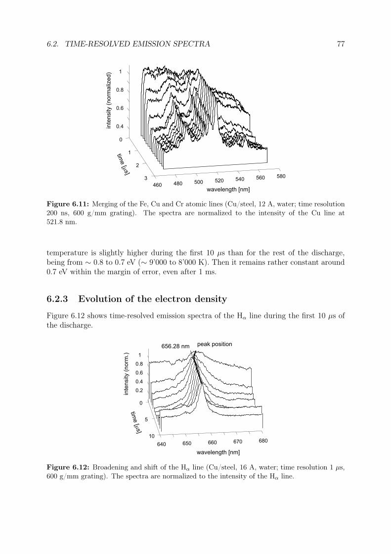
6.2. TIME-RESOLVED EMISSION SPECTRA 77
wavelength [nm]
time
[s]
m
0
1
2
3
460 480 500 520 540 560 580
0.4
0.6
0.8
1
inte
nsity (
norm
aliz
ed)
Figure 6.11: Merging of the Fe, Cu and Cr atomic lines (Cu/steel, 12 A, water; time resolution200 ns, 600 g/mm grating). The spectra are normalized to the intensity of the Cu line at521.8 nm.
temperature is slightly higher during the first 10 µs than for the rest of the discharge,being from ∼ 0.8 to 0.7 eV (∼ 9’000 to 8’000 K). Then it remains rather constant around0.7 eV within the margin of error, even after 1 ms.
6.2.3 Evolution of the electron density
Figure 6.12 shows time-resolved emission spectra of the Hα line during the first 10 µs ofthe discharge.
640 650 660 670 680
0
5
10
656.28 nm peak position
wavelength [nm]
time
[s]
m
0.2
0.4
0.6
0.8
1
inte
nsity (
norm
.)
Figure 6.12: Broadening and shift of the Hα line (Cu/steel, 16 A, water; time resolution 1 µs,600 g/mm grating). The spectra are normalized to the intensity of the Hα line.

78 CHAPTER 6. OPTICAL EMISSION SPECTROSCOPY OF EDM PLASMAS
The very first spectra show extremely broadened and shifted Hα lines. Thus, it isquite difficult to find a good fit for the first spectra, leading to non negligible errors in theFWHM measurements. The black lines on figure 6.12 represent the theoretical positionof the Hα line (656.28 nm) and the measured peak positions. These lines are drawn toeasily visualize the line shift. At the beginning of the discharge, we can measure FWHMup to 10 nm and shift up to 10 Å.
The evolution of ne is calculated from these time-resolved Hα spectra with equa-tions (3.6) and (3.7). Results are given in figure 6.13.
1 10 100
broadeningshift
time [ s]m
ele
ctro
n d
ensi
ty [cm
]-3
1018
1017
Figure 6.13: Evolution of the electron density, deduced from time-resolved broadening andshift measurements of the Hα line (Cu/steel, 16 A, water).
In spite of some differences, the FWHM and the shift measurements give comparabledensity values and evolution. As expected, the electron density is extremely high duringthe first microsecond (above 1018 cm−3) and then decreases rapidly with time. The EDMplasma is created from a liquid, which is a dense medium (∼ 3·1022 water molecules/cm3,for example). This is the main reason for the high plasma density. In the very beginning ofthe discharge, the plasma has to overcome the extreme pressure imposed by the dielectric.Then the plasma expands, which results in a decrease in its density. But during the wholedischarge, the density remains high (always above 1016 cm−3) due to the constant pressureof the surrounding liquid. The density reduction with time is confirmed by other studieson discharges in liquids [34].
The high electron density measured reinforces the assumption of free-bound and free-free radiation for the explanation of the continuum given in § 6.1.1. Since these twotypes of radiation processes involve free electrons, the intensity of free-bound and free-free radiation is in fact directly related to ne. Therefore, the continuum is expected to beintense with such high values of ne. Moreover, the measured continuum decreases withthe discharge on-time (see figure 6.9), which is consistent with the decrease of ne withtime.

6.3. SPATIALLY-RESOLVED EMISSION SPECTRA 79
6.3 Spatially-resolved emission spectraFigure 6.14 shows an example of spatially-resolved spectra along the vertical axis. Theintensities of the spectra located in the center are higher, because the plasma is brighterin this region (see also figure 5.6).
450 500 550 600 650 700
5
10
15# fibre
wavelength [nm]
inte
nsity [arb
. un
it]
Figure 6.14: Example of spatially-resolved spectra, along the vertical axis (Cu/steel, 12 A,4 µs, water, 150 g/mm grating).
Note that the spatially-resolved axis is not calibrated in real distance, but simplygraduated with the numbers of the fibres making the sampling. In order to make theconversion into real distance, we have to know the spatial resolution obtained with thefibre bundle, i.e. the real distance between two points seen by two consecutive fibres. Thisspatial resolution depends on the optical arrangement, mostly on the plasma−endoscopedistance, which is not constant from one set of measurements to another. After eachset of measurements (the simultaneous acquisition of the 16 spectra), the electrodes haveto be changed due to their erosion, and the optical arrangement has to be re-aligned.Thus, an exact calibration for each set of measurements is time-consuming and has notbeen systematically done. The spatial resolution can nevertheless be estimated around20−30 µm/fibre (gap distance ∼ 100 µm), for all the measurements presented here.
6.3.1 Asymmetry of the contamination
As previously said, the spectral region around 520 nm is interesting for a qualitativecharacterization of the plasma contamination, because of the presence of three chromiumlines at 520.45, 520.6 and 520.84 nm, and of the copper line at 521.82 nm. With a copperelectrode and a stainless steel workpiece, the Cu line is emitted by particles comingfrom the electrode and the Cr lines are emitted by particles coming from the workpiece.Figure 6.15 shows spatially-resolved spectra along the vertical axis of this spectral region.

80 CHAPTER 6. OPTICAL EMISSION SPECTROSCOPY OF EDM PLASMAS
500 510 520 530 540 550
67891011
0
0.2
0.4
0.6
0.8
1
# fibrewavelength [nm]
inte
nsity (
norm
aliz
ed)
Cu line (=1)
Cr line
to steelelectrode
to copperelectrode
Figure 6.15: Vertical asymmetry of the plasma contamination (Cu/steel, 6 A, 100 µs, water,150 g/mm grating). The spectra are normalized to the intensity of the Cu line at 521.8 nm.
An asymmetry of the plasma contamination is clearly visible. Near the Cu electrode,the Cu line is more intense than the Cr lines. On the other hand, the Cr lines are moreintense than the Cu line near the steel workpiece. Thus, even if Cu and Cr lines are presenteverywhere in the plasma, we see that each electrode is contaminating the plasma mostlyin a region close to itself. Unsurprisingly, no asymmetry is visible along the horizontalaxis (measurement not shown here).
Depending on the discharge parameters, material transfer from one electrode to theother can sometimes be observed. In this case, the intensity of lines emitted by bothelectrode materials are quite constant across the vertical profile. With the dischargeconditions of figure 6.15, no material transfer is macroscopically visible on the electrodesafter several minutes of machining. This is qualitatively confirmed by the contaminationasymmetry measured by spatially-resolved spectroscopy.
6.3.2 Electron temperature profile
Spatially-resolved spectra of the three Cu lines used for Te calculations are shown infigure 6.16, along with the electron temperature vertical profile calculated from them.The central spectra have a better signal to noise ratio than the outer ones, because thelight intensity is higher in the center. The electron temperature is quite constant overthe whole profile. Measurements along the horizontal axis are not shown here but do notshow any difference. The plasma has thus a homogeneous electron temperature around0.7 eV, as previously measured.
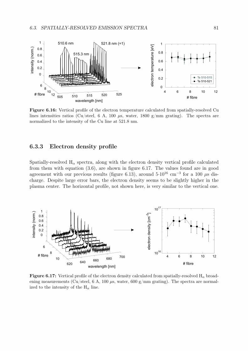
6.3. SPATIALLY-RESOLVED EMISSION SPECTRA 81
505 510 515 520 525
68
1012
0
0.2
0.4
0.6
0.8
1
wavelength [nm]
# fibre# fibre
inte
nsity (
norm
.)
0
0.2
0.4
0.6
0.8
1
4 6 8 10 12
ele
ctr
on tem
pera
ture
[eV
]521.8 nm (=1)
515.3 nm
510.6 nm
Te 510-515
Te 510-521
Figure 6.16: Vertical profile of the electron temperature calculated from spatially-resolved Culines intensities ratios (Cu/steel, 6 A, 100 µs, water, 1800 g/mm grating). The spectra arenormalized to the intensity of the Cu line at 521.8 nm.
6.3.3 Electron density profile
Spatially-resolved Hα spectra, along with the electron density vertical profile calculatedfrom them with equation (3.6), are shown in figure 6.17. The values found are in goodagreement with our previous results (figure 6.13), around 5·1016 cm−3 for a 100 µs dis-charge. Despite large error bars, the electron density seems to be slightly higher in theplasma center. The horizontal profile, not shown here, is very similar to the vertical one.
620 640 660 680 700
6
8
10
0
0.2
0.4
0.6
0.8
1
wavelength [nm]
# fibre 4 6 8 10 12
# fibre
inte
nsi
ty (
norm
.)
ele
ctro
n d
ensi
ty [cm
]-3
1016
1017
Figure 6.17: Vertical profile of the electron density calculated from spatially-resolved Hα broad-ening measurements (Cu/steel, 6 A, 100 µs, water, 600 g/mm grating). The spectra are normal-ized to the intensity of the Hα line.
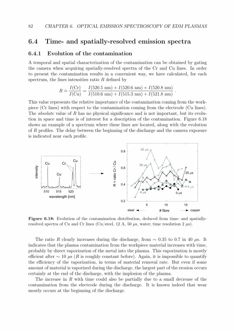
82 CHAPTER 6. OPTICAL EMISSION SPECTROSCOPY OF EDM PLASMAS
6.4 Time- and spatially-resolved emission spectra
6.4.1 Evolution of the contamination
A temporal and spatial characterization of the contamination can be obtained by gatingthe camera when acquiring spatially-resolved spectra of the Cr and Cu lines. In orderto present the contamination results in a convenient way, we have calculated, for eachspectrum, the lines intensities ratio R defined by
R.=
I(Cr)I(Cu)
=I(520.5 nm) + I(520.6 nm) + I(520.8 nm)
I(510.6 nm) + I(515.3 nm) + I(521.8 nm).
This value represents the relative importance of the contamination coming from the work-piece (Cr lines) with respect to the contamination coming from the electrode (Cu lines).The absolute value of R has no physical significance and is not important, but its evolu-tion in space and time is of interest for a description of the contamination. Figure 6.18shows an example of a spectrum where these lines are located, along with the evolutionof R profiles. The delay between the beginning of the discharge and the camera exposureis indicated near each profile.
0.2
0.4
0.6
0.8
5 10 15
510 515 520
# fibre
wavelength [nm]
inte
nsity
Cu Cr
Cu
Cu
R =
ratio C
r / C
u
0 sm
20 sm
30 sm
40 sm
4 sm
8 sm
steel copper
Figure 6.18: Evolution of the contamination distribution, deduced from time- and spatially-resolved spectra of Cu and Cr lines (Cu/steel, 12 A, 50 µs, water; time resolution 2 µs).
The ratio R clearly increases during the discharge, from ∼ 0.35 to 0.7 in 40 µs. Itindicates that the plasma contamination from the workpiece material increases with time,probably by direct vaporization of the metal into the plasma. This vaporization is mostlyefficient after ∼ 10 µs (R is roughly constant before). Again, it is impossible to quantifythe efficiency of the vaporization, in terms of material removal rate. But even if someamount of material is vaporized during the discharge, the largest part of the erosion occurscertainly at the end of the discharge, with the implosion of the plasma.
The increase in R with time could also be partially due to a small decrease of thecontamination from the electrode during the discharge. It is known indeed that wearmostly occurs at the beginning of the discharge.
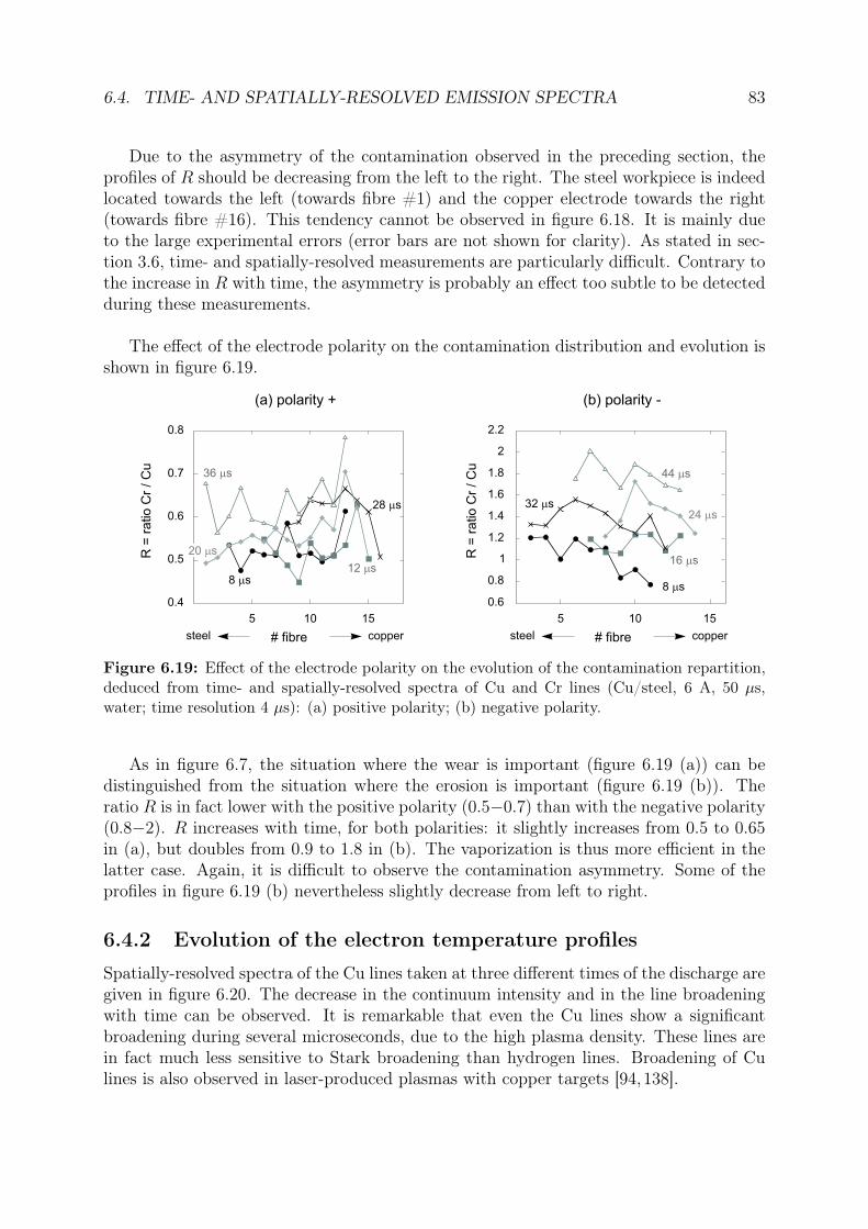
6.4. TIME- AND SPATIALLY-RESOLVED EMISSION SPECTRA 83
Due to the asymmetry of the contamination observed in the preceding section, theprofiles of R should be decreasing from the left to the right. The steel workpiece is indeedlocated towards the left (towards fibre #1) and the copper electrode towards the right(towards fibre #16). This tendency cannot be observed in figure 6.18. It is mainly dueto the large experimental errors (error bars are not shown for clarity). As stated in sec-tion 3.6, time- and spatially-resolved measurements are particularly difficult. Contrary tothe increase in R with time, the asymmetry is probably an effect too subtle to be detectedduring these measurements.
The effect of the electrode polarity on the contamination distribution and evolution isshown in figure 6.19.
0.4
0.5
0.6
0.7
0.8
0.6
0.8
1
1.2
1.4
1.6
1.8
2
2.2
5 10 15
# fibre
R =
ratio C
r / C
u
steel copper
R =
ratio C
r / C
u
5 10 15
# fibresteel copper
(a) polarity + (b) polarity -
8 sm
12 sm
28 sm
36 sm
20 sm
8 sm
16 sm
24 sm
44 sm
32 sm
Figure 6.19: Effect of the electrode polarity on the evolution of the contamination repartition,deduced from time- and spatially-resolved spectra of Cu and Cr lines (Cu/steel, 6 A, 50 µs,water; time resolution 4 µs): (a) positive polarity; (b) negative polarity.
As in figure 6.7, the situation where the wear is important (figure 6.19 (a)) can bedistinguished from the situation where the erosion is important (figure 6.19 (b)). Theratio R is in fact lower with the positive polarity (0.5−0.7) than with the negative polarity(0.8−2). R increases with time, for both polarities: it slightly increases from 0.5 to 0.65in (a), but doubles from 0.9 to 1.8 in (b). The vaporization is thus more efficient in thelatter case. Again, it is difficult to observe the contamination asymmetry. Some of theprofiles in figure 6.19 (b) nevertheless slightly decrease from left to right.
6.4.2 Evolution of the electron temperature profiles
Spatially-resolved spectra of the Cu lines taken at three different times of the discharge aregiven in figure 6.20. The decrease in the continuum intensity and in the line broadeningwith time can be observed. It is remarkable that even the Cu lines show a significantbroadening during several microseconds, due to the high plasma density. These lines arein fact much less sensitive to Stark broadening than hydrogen lines. Broadening of Culines is also observed in laser-produced plasmas with copper targets [94, 138].

84 CHAPTER 6. OPTICAL EMISSION SPECTROSCOPY OF EDM PLASMAS
(a) 0 to 2 sm (c) 48 to 50 sm(b) 4 to 6 sm
500510
520
510
15
wavelength [nm]# fibre
500510
520
510
15500
510520
510
15
Figure 6.20: Time- and spatially-resolved spectra of the Cu lines used for electron temperaturecalculation (Cu/steel, 12 A, 50 µs, water; time resolution 2 µs, 600 g/mm grating): (a) 0 to 2 µs;(b) 4 to 6 µs; (c) 48 to 50 µs.
Figure 6.21 shows the evolution of Te profiles calculated from the previous spectra. Aspreviously mentioned, the electron temperature is slightly higher at the beginning, butremains around 0.7 eV. The profiles are roughly flat within the margin of errors.
0.5
0.6
0.7
0.8
0.9
0 4 8 12 16
# fibre
ele
ctr
on tem
pera
ture
[eV
]
8 sm
12 sm
16 sm
48 sm
28 sm
Figure 6.21: Evolution of the electron temperature profiles (Cu/steel, 12 A, 50 µs, water, timeresolution 2 µs).
6.4.3 Evolution of the electron density profiles
Time- and spatially-resolved Hα spectra are shown in figure 6.22. The spectra are quitenoisy, due to the weak intensity emitted. Nevertheless, the Hα broadening is easily ob-servable.
The evolution of the electron density profiles is presented in figure 6.23. These den-sity measurements are consistent with time-resolved and spatially-resolved measurements

6.4. TIME- AND SPATIALLY-RESOLVED EMISSION SPECTRA 85
(a) 0 to 2 sm (c) 36 to 38 sm(b) 4 to 6 sm
640650
6605
1015# fibre
wavelength [nm]640
650660
510
15
640650
6605
1015
Figure 6.22: Time- and spatially-resolved spectra of the Hα line (Cu/steel, 12 A, 50 µs, water;time resolution 2 µs, 600 g/mm grating): (a) 0 to 2 µs; (b) 4 to 6 µs; (c) 36 to 38 µs.
previously presented (figures 6.13 and 6.17). The density diminishes during the discharge,by almost two orders of magnitude in 50 µs. The density is slightly higher in the plasmacenter, and this tendency is verified during the whole discharge. This temporal and spatialcharacterization of ne can be useful for the validation of EDM plasma simulations.
4 6 8 10 12 14
# fibre
1018
1017
1016
ele
ctro
n d
ensi
ty [cm
]-3
0 sm
12 sm
4 sm
8 sm
16 sm
20 sm
48 sm
36 sm
Figure 6.23: Evolution of the electron density profiles (Cu/steel, 12 A, 50 µs, water, timeresolution 2 µs).

86 CHAPTER 6. OPTICAL EMISSION SPECTROSCOPY OF EDM PLASMAS
Chapter 7
Non-ideality of EDM plasmas
In this chapter, we will show that EDM plasmas are weakly non-ideal. The definition ofa non-ideal plasma is given in the first section. Spectroscopic evidence of the non-idealityof EDM plasmas is discussed in the second section. Finally, the third section presents ageneral summary of the EDM plasma physical properties, measured in this work.
7.1 Plasma coupling parameter Γ
Natural plasmas and artificially-produced plasmas are both very diverse. Generally, theyare classified according to their temperature and density, because the properties of aplasma depend mostly on these two parameters.
In particular, the density n and temperature T define whether a plasma is ideal ornot. In an ideal plasma, the particles are almost free, i.e. their movement is only weaklyinfluenced by other particles. In this case, the mean kinetic energy of particles is muchhigher than the mean Coulomb potential energy between them.
Knowing n and T for a given plasma, we can calculate its coupling parameter Γ, whichquantifies its “degree of ideality”. This parameter represents the ratio of the potentialenergy of Coulomb interaction at the mean inter-particle distance divided by the meanthermal energy of the charged particles in the plasma. It is defined by
Γ.=
Z2e2
4πε0 a kBT, (7.1)
where Z is the charge of the particles (Z=1 for hydrogen ions, for example), e the ele-mentary charge, ε0 the vacuum permittivity, and a the mean inter-particle distance givenby
a =
(3
4πn
)1/3
. (7.2)
Therefore, we see that
Γ ∝ n1/3
T. (7.3)
87

88 CHAPTER 7. NON-IDEALITY OF EDM PLASMAS
The plasma is called:
• ideal if Γ ¿ 1;
• weakly non-ideal if Γ ≤ 1;
• strongly coupled if Γ > 1.
According to equation (7.3), we see that ideal plasmas are characterized by a low densityand a high temperature. Note that Γ is linked with the Debye length λD, defined by
λD.=
√ε0 kBT
e2 n, (7.4)
by the relation
Γ 3/2 ∝ 1
nλ3D
.
Therefore, we see also that, in an ideal plasma, a very large number of particles is con-tained in a Debye sphere. Nevertheless, the higher the number of particles in a Debyesphere, the less the particles interact with each other.
On the other hand, non-ideal and strongly coupled plasmas are dense and/or cold. Insuch plasmas, the inter-particle distance is short enough, and the particle velocity smallenough, to produce significant electrostatic interactions between the charged particles.For a given particle, the microfields created by the others have a significant influence onit.
We have seen in the previous chapter that EDM plasmas have a typical electron tem-perature of 0.7 eV and a typical electron density of 1018 cm−3. Thus, the typical couplingparameter of EDM plasmas is around
Γ ' 0.33 .
If we consider that ne reaches 2.5 · 1018 cm−3 in the very beginning of the discharge (seefigure 6.13), Γ ' 0.45 during the first microsecond. Thus, EDM discharges produce coldand dense plasmas which are weakly non-ideal.
According to equation (7.4), the typical Debye length of EDM plasmas is around 6 nm.The mean inter-particle distance a is also around 6 nm (equation (7.2)). Thus, a Debyesphere is containing roughly only one particle. This is another illustration of the plasmanon-ideality.
Figure 7.1 shows the classification of the main types of natural and artificial plasmas,including EDM plasmas, in a log density−log temperature diagram. Ideal, weakly non-ideal and strongly coupled plasmas can easily be distinguished in such a log-log diagram,because Γ iso-contours are straight lines.

7.1. PLASMA COUPLING PARAMETER Γ 89
log T [eV]
- 2 - 1 0 1 2 3 4 5
log n
[cm
]-3
25
20
15
10
5
0
Earthplasma sheet
Solar wind(1 AU)
Earthiono-
sphere
Flames
Glowdischarge
Solarcorona
Lowpressure
Alkalimetal
plasma
Fusionexperiments
Fusionreactor
Focus
Z-pinches
Laserplasma
Shocktubes
High pressurearcs
EDM
strongly-coupledplasmas
ideal plasmas
wea
kly
non-
idea
l
plas
masJupiter core
30
Sun core
white dwarf
brown dwarf
G=
0.01
G=
0.1
G=
1G
=10
Interstellar gas
activegalacticnucleus
6
log T [K]
2 3 4 5 6 7 8 9 10
Figure 7.1: Classification of plasmas according to their density and temperature (adaptedfrom [45,139]).
One can see in figure 7.1 that the majority of natural and artificial plasmas are ideal.Besides extremely dense astrophysical objects, few non-ideal plasmas exist. From thephysical point of view, their extreme properties make them particularly interesting tostudy. The physics of non-ideal plasmas is complex, differing from “classical” plasma

90 CHAPTER 7. NON-IDEALITY OF EDM PLASMAS
physics theories [43–46]. Corrections have to be made because of deviations from thebinary collision model due to collective effects. For example, the screening mechanismdescribed by the Debye model has to be modified in non-ideal plasmas. Theories havebeen developed quite recently, mainly due to the lack of experimental data before the1980’s. The creation of dense, and therefore non-ideal plasmas, is in fact difficult andrequires considerable experimental resources (see § 2.3). In this context, EDM dischargesappear to be a very simple method to produce such plasmas. EDM plasmas are indeedamongst the most dense artificially-created plasmas. But unfortunately, these plasmasare not the easiest to be investigated experimentally, as repeated several times in thiswork.
7.2 Spectroscopic signs of the non-ideality
In addition, spectroscopic results indicate also that the EDM plasma is non-ideal.
7.2.1 Broadening and shift of Hα
Since non-ideal plasmas are dense, a strong Stark broadening and shift of spectral lines isnaturally a characteristic sign of non-ideality. The microfields deform the energy spectrumof radiating atomic particles, i.e. they perturb the initial and final states of radiativetransitions. The atomic levels are shifted and split, and this results in line broadeningand shift [43,44].
This effect can be clearly observed on optical spectra emitted by EDM plasmas, espe-cially on the Hα line. This fact has already been discussed in detail in chapter 6. Similarstrong broadening and shift of hydrogen lines in dense plasmas have been reported innumerous works [113,115,117,135,140–144].
It should be noted that the calculation of spectral line shapes emitted by dense plasmashas been recently much improved. Simulations in good agreement with experimentaldata are obtained with models including several non-ideal effects, such as the effect ofthe dynamic microfield created by the ions or the influence of electron collisions [45].Calculations are mostly done for lines of the hydrogen atom or hydrogen-like ions, becauseof the “simplicity” of quantum calculations for these species.
7.2.2 Asymmetry and structure of Hα
Besides its broadening and shift, the Hα line gives other useful information. Figure 7.2shows a typical example of a high resolution spectrum of the Hα line. If a lorentzian fitis applied, it is observed that the shape of the line is slightly asymmetric and deviatesfrom the fit. This asymmetry is also due to interactions between ions and the emitter(hydrogen atom in our case), and is another sign of plasma non-ideality [43,114,116].
We also see in figure 7.2 the complex structures around the Hα line. The arrows marksmall bumps which are not due to radiation of other lines. These structures are createdby several phenomena, which occur in dense plasmas [145–153]. Figure 7.3 gives a simpleexplanation for the origin of these structures.
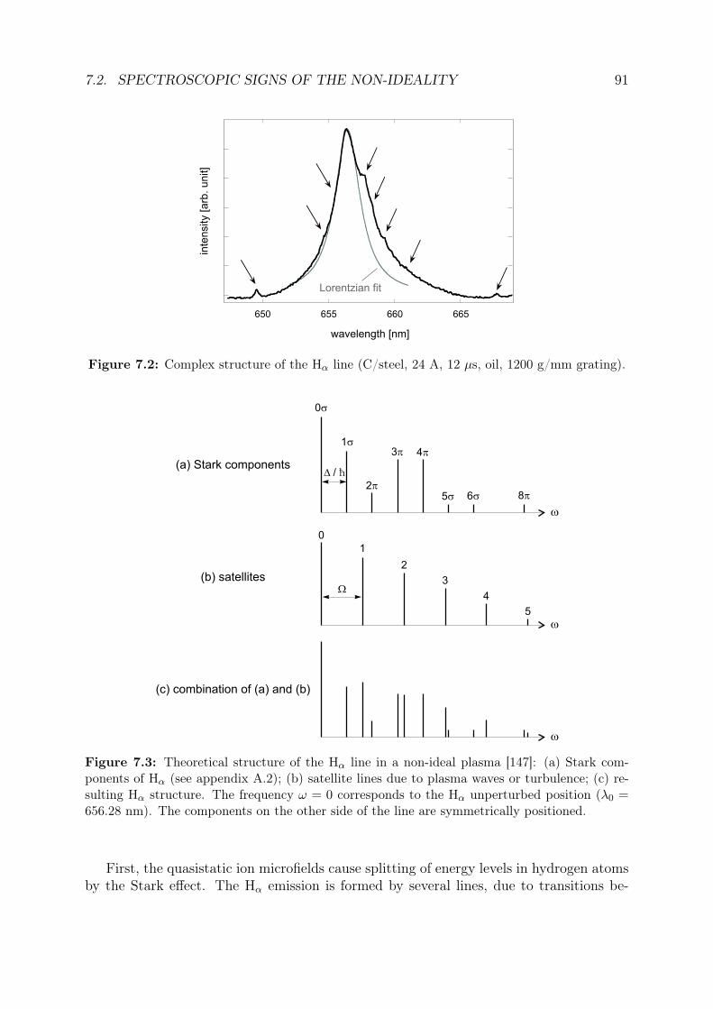
7.2. SPECTROSCOPIC SIGNS OF THE NON-IDEALITY 91
wavelength [nm]
inte
nsity [arb
. unit]
650 655 660 665
Lorentzian fit
Figure 7.2: Complex structure of the Hα line (C/steel, 24 A, 12 µs, oil, 1200 g/mm grating).
w
0s
1s
2p
3p 4p
5s 6s 8p
(a) Stark components
w
(b) satellites
w
(c) combination of (a) and (b)
1
2
3
4
5
0
W
D / ħ
Figure 7.3: Theoretical structure of the Hα line in a non-ideal plasma [147]: (a) Stark com-ponents of Hα (see appendix A.2); (b) satellite lines due to plasma waves or turbulence; (c) re-sulting Hα structure. The frequency ω = 0 corresponds to the Hα unperturbed position (λ0 =656.28 nm). The components on the other side of the line are symmetrically positioned.
First, the quasistatic ion microfields cause splitting of energy levels in hydrogen atomsby the Stark effect. The Hα emission is formed by several lines, due to transitions be-
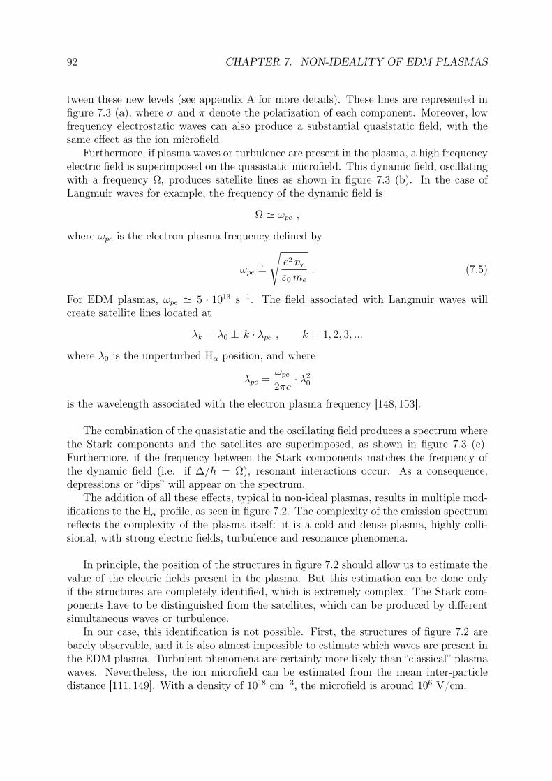
92 CHAPTER 7. NON-IDEALITY OF EDM PLASMAS
tween these new levels (see appendix A for more details). These lines are represented infigure 7.3 (a), where σ and π denote the polarization of each component. Moreover, lowfrequency electrostatic waves can also produce a substantial quasistatic field, with thesame effect as the ion microfield.
Furthermore, if plasma waves or turbulence are present in the plasma, a high frequencyelectric field is superimposed on the quasistatic microfield. This dynamic field, oscillatingwith a frequency Ω, produces satellite lines as shown in figure 7.3 (b). In the case ofLangmuir waves for example, the frequency of the dynamic field is
Ω ' ωpe ,
where ωpe is the electron plasma frequency defined by
ωpe.=
√e2 ne
ε0 me
. (7.5)
For EDM plasmas, ωpe ' 5 · 1013 s−1. The field associated with Langmuir waves willcreate satellite lines located at
λk = λ0 ± k · λpe , k = 1, 2, 3, ...
where λ0 is the unperturbed Hα position, and where
λpe =ωpe
2πc· λ2
0
is the wavelength associated with the electron plasma frequency [148,153].
The combination of the quasistatic and the oscillating field produces a spectrum wherethe Stark components and the satellites are superimposed, as shown in figure 7.3 (c).Furthermore, if the frequency between the Stark components matches the frequency ofthe dynamic field (i.e. if ∆/~ = Ω), resonant interactions occur. As a consequence,depressions or “dips” will appear on the spectrum.
The addition of all these effects, typical in non-ideal plasmas, results in multiple mod-ifications to the Hα profile, as seen in figure 7.2. The complexity of the emission spectrumreflects the complexity of the plasma itself: it is a cold and dense plasma, highly colli-sional, with strong electric fields, turbulence and resonance phenomena.
In principle, the position of the structures in figure 7.2 should allow us to estimate thevalue of the electric fields present in the plasma. But this estimation can be done onlyif the structures are completely identified, which is extremely complex. The Stark com-ponents have to be distinguished from the satellites, which can be produced by differentsimultaneous waves or turbulence.
In our case, this identification is not possible. First, the structures of figure 7.2 arebarely observable, and it is also almost impossible to estimate which waves are present inthe EDM plasma. Turbulent phenomena are certainly more likely than “classical” plasmawaves. Nevertheless, the ion microfield can be estimated from the mean inter-particledistance [111,149]. With a density of 1018 cm−3, the microfield is around 106 V/cm.

7.2. SPECTROSCOPIC SIGNS OF THE NON-IDEALITY 93
7.2.3 Absence of Hβ and line merging
Another important effect of the plasma non-ideality is the transformation of the uppermembers of a spectral series into a continuous spectrum [43, 44, 134]. This effect is dueto:
1. the lowering of the ionization threshold;
2. the merging of spectral lines near the series limit.
First, the ionization potential of atoms is lowered in non-ideal plasmas. Inter-particleinteractions in high density plasmas “destroy” in fact the upper atomic levels. Moreprecisely, the microfields which are superimposed on the Coulomb electric field of anatomic nucleus, transform the upper energy states of this atom into unbound states, asshown in figure 7.4.
r
V(r)
(1) Coulomb potential
(2) microfield
unbound states
bound states
(1) + (2)
Figure 7.4: Lowering of the ionization threshold in non-ideal plasmas, due to the effect ofmicrofields (assumed to be uniform on the atomic scale) [44].
The shift in the ionization energy ∆Ui is given by
∆Ui =Z2e2
4πε0 λD
, (7.6)
where λD is the Debye length [44,46]. In our case, we found ∆Ui ' 0.23 eV. This loweringof the ionization threshold modifies the optical spectrum of the plasma. Figure 7.5 explainsschematically the consequences in the case of an hydrogen plasma.
In an unperturbed atom, all the levels can be populated by electrons (figure 7.5 (a)).Therefore, the different lines of all series can be emitted, in particular those of the Balmerseries: Hα, Hβ, Hγ, etc. Continuous radiation by free-bound transitions is emitted byelectrons coming from the energy continuum, whose threshold is 13.6 eV above the groundstate n = 1 (see figure 3.8).
On the other hand, in a dense plasma, the ionization potential is lowered due to themicrofields. If the “new” threshold is located between levels n = 3 and n = 4 for example

94 CHAPTER 7. NON-IDEALITY OF EDM PLASMAS
n=2
n=3
n=4
n=5
Ha
Hb
Hg
ionization threshold
Ha
continuum
(a) unperturbed H atom (b) H atom in a dense plasma
continuumradiation
continuumradiation
n=2
n=3
ionization threshold
Figure 7.5: Absence of Hβ and increase in the continuum radiation due to the lowering of theionization threshold in a dense hydrogen plasma.
(figure 7.5 (b)), the only Balmer line which can still be emitted is the Hα line, becausethe upper levels of all other Balmer lines are now in the energy continuum. In additionto the disappearance of these lines, another consequence of the lowering of the ionizationthreshold is an increase in the continuum radiation. Free-bound and free-free transitionsbecome much more likely with a lowered threshold.
Secondly, some of the remaining spectral lines, whose upper states are yet below the“new” ionization threshold, can still be “erased”. Although these lines are discrete transi-tions, they appear as a continuum radiation not because their upper state is in the energycontinuum, but because of the Stark broadening. The upper lines of a series are closeto each other in the spectrum. If they are significantly broadened so that their widthsexceed the distance between them, they will overlap with adjacent lines and merge into acontinuum. The continuum formed by this degeneracy of lines is the type of continuumobserved during the first microsecond of the EDM discharge (see § 6.1.6 and § 6.2.1). TheStark broadening of lines near the series limit has thus the same effect as the loweringof the ionization threshold: it transforms the upper members of a spectral series into acontinuous spectrum. Therefore, this second effect can be considered as an apparent oroptical lowering of the ionization threshold [43,44].
As showed in chapter 6, the spectra of EDM plasmas are characterized by the absenceof the Hβ line and other upper Balmer lines, by an strong continuum radiation and bymerging of almost all lines at the beginning of the discharge. All these characteristics canthus be viewed as signs of the non-ideality of the EDM plasma.
7.2.4 Inglis-Teller relation
As previously said, upper spectral lines of a series can be merged if the plasma is dense,due to their overlapping caused by Stark broadening. Since the number of these “erased”
7.3. SUMMARY OF THE PHYSICAL PROPERTIES OF EDM PLASMAS 95
lines depends on the plasma density, the last discernible line gives a rough estimationof the density. For hydrogen Balmer lines, this estimation is given by the Inglis-Tellerrelation:
log n = 23.26− 7.5 · log nmax , (7.7)
where n is the density expressed in cm−3 and nmax the quantum number of the upperenergy level of the last visible transition [43,108,154–156]. This relation is mainly used inastrophysics, to evaluate the electron density in the atmosphere of stars, for example. Thecoefficients of this relation are sometimes slightly different in literature. The uncertaintyfactor of this relation is about 50% [108].
If we observe on EDM spectra the Hα line (transition from level 3 to 2) but no Hβ line(transition from level 4 to 2), then
3 ≤ nmax < 4 ,
and the plasma density is at least 6·1018 cm−3 according to relation (7.7). This roughestimation is of the same order of magnitude as our previous density measurements andconfirms their validity.
Contrary to upper hydrogen Balmer lines which disappear because of their strongbroadening, metallic lines do not merge and can be observed in the EDM plasma spectrum,as shown in chapter 6. The metallic lines are much less sensitive to Stark broadening, andthis explains why they are still observable. The Stark broadening of non-hydrogenic linesis rather poorly documented, and few data are available [157]. Nevertheless, the FWHM ofa few atomic copper lines can be found. For example, in a plasma with an electron densityof 1017 cm−3 and at 10’000 K, the FWHM of the Hα line is 10.8 Å, whereas the FWHM ofthe Cu lines at 510.6, 515.3 and 521.8 nm are 0.43, 1.9 and 2.2 Å respectively [158]. Thisshows that non-hydrogenic lines are not sufficiently broadened to merge and disappearinto a continuum, as upper hydrogen lines do.
7.3 Summary of the physical properties of EDM plas-mas
According to the measurements presented in this work, EDM plasmas have the followingcharacteristics:
• The plasma is composed of species coming from the cracking of the dielectricmolecules, mainly hydrogen, with contamination from the electrode materials.The contamination is slightly higher in the vicinity of the electrodes, and increasesduring the discharge.
• The electron temperature Te is low, around 0.7 eV (8’100 K), slightly higher atthe beginning of the discharge. The temperature is homogeneous in the plasma. The
96 CHAPTER 7. NON-IDEALITY OF EDM PLASMAS
assumption of LTE can be accepted due to the high plasma density, and thereforethe ion temperature Ti should be similar to the electron temperature.
• The electron density ne is extremely high, reaching 2·1018 cm−3 during the firstmicrosecond of the discharge, decreasing rapidly afterwards. The density is slightlyhigher in the plasma center. The ion density ni should be roughly equal to the elec-tron density, since multiple ions are unlikely with such a low electron temperatureand since quasineutrality should hold.
• The plasma is very dense and cold, and therefore presents several non-ideal effects,especially in the beginning of the discharge. The coupling parameter Γ is around0.33, and reaches 0.45 during the first microsecond.
• The Debye length λD is around 6 nm, and the mean inter-particle distance ais also around 6 nm. Therefore, a Debye sphere contains roughly only one particle.Again, this is a sign of the plasma non-ideality.
• The light emitted by the plasma is much more intense during the first microsecondthan during the rest of the discharge.
• Due to its high density, the EDM plasma could be not completely optically thin.The opacity of a plasma increases in fact with the density. For example, ultra-dense plasmas produced by exploding wires in water (ne = 2 · 1021 cm−3) are knownto be highly opaque and to radiate like a blackbody [33]. Consequently, the lightemitted by the very center of the EDM plasma at the beginning of the dischargecould be absorbed within the plasma and not be measured. The opacity can be aproblem for spectroscopic diagnostics, since the core of an opaque plasma cannot becharacterized with such diagnostics. Nevertheless, in our case, the plasma opacitycould be critical only during roughly the first 500 ns of the discharge, when thedensity reaches its maximum. But during this period, Te and ne can anyway notbe measured with the spectroscopic methods used in this work, because of the linemerging.
• Energy is dissipated in the plasma by Joule heating, heat conduction, radiation andmechanical work (plasma expansion). Energy is also used for evaporation, dissoci-ation, ionization and excitation of the dielectric molecules and atoms. The energyreceived by the workpiece is mainly brought by ion bombardment. Thermal run-away of the very superficial layers is also probable in the beginning of the discharge,due to the massive flow of energy at the breakdown.
• For a plasma in LTE, the repartition of the densities of the different species is de-scribed by the Saha equation. For a plasma containing electrons, one type of singlycharged ions and one type of atoms, the Saha equation is
ne ni
na
=Ze Zi
Za
·(
2πme kBT
h2
)3/2
· exp
(−Ui −∆Ui
kBT
), (7.8)
7.3. SUMMARY OF THE PHYSICAL PROPERTIES OF EDM PLASMAS 97
where nk is the density of the species k, Zk its partition function, Ui the ionization en-ergy of the atom, and ∆Ui its correction due to non-ideality (equation (7.6)) [44,159].In principle, this equation can be used for the calculation of the EDM plasma ion-ization degree ne/na. For a hydrogen plasma, Ze = 2, Zi = 1 and
Za =nmax∑n=1
gn exp
(− En
kBT
)=
nmax∑n=1
2n2 exp
(−Ui (1− 1/n2)
kBT
),
where Ui = 13.6 eV and n2max = Ui/∆Ui. In our case, we found Za ' 2. Assuming
in addition ne = ni = 1018 cm−3, we found ne/na = 10−5.
The ionization degree of the EDM plasma is certainly much higher, probably about0.1 as for similar discharges [34]. High-pressure arcs have also similar densitiesas EDM plasmas, and are known to be strongly ionized. The calculation givesne/na = 10−5, then we found na = 1023 cm−3 if we assume that ne = 1018 cm−3.Such a high density of atoms is unlikely, since the density of molecules in the liquidis around 1022 cm−3. This shows that the ionization degree calculated here is notcorrect. The assumptions made are probably too strong. In particular, the Sahaequation as written in (7.8) does not take into account the complex composition ofthe EDM plasma. But for a multi-component plasma, the Saha equation has noanalytical solution and becomes difficult to solve [159].
• Assuming a temperature of 0.7 eV, a density of 2·1018 cm−3 and that the plasma isa fully ionized hydrogen plasma, the plasma pressure p at the beginning of thedischarge is
p = p ideal −∆p = (ne + ni) kB T −∆p ,
where ∆p is a correction due to the plasma non-ideality [44,46] given by
∆p =e2
24πε0 λD
· (ne + ni) .
We found that p ' 4.2 bar. Since the density decreases during the discharge, thepressure is also decreasing. The value found is lower than the pressure calculatedwith the simulation [40] (∼ 103 bar). But the assumption of a fully ionized hy-drogen plasma is obviously a simplification. In reality, the plasma composition ismore complex and the plasma is partially ionized (the Hα line is emitted by neutralhydrogen atoms). The pressure is thus higher than 4.2 bar, depending on the ion-ization degree of the plasma. Nevertheless, the pressure is still much lower than thevalue found with the simulation.
• The estimated dimensions of the plasma are summarized in figure 7.6. The elec-trode gap is around 100 µm, and the plasma radius in the middle of the gap is alsoaround 100− 200 µm, growing with time. The contact surface between the plasma

98 CHAPTER 7. NON-IDEALITY OF EDM PLASMAS
and the electrodes can be estimated from measurements of crater diameter, andis ∼ 10 µm. Therefore, the current density j flowing through the plasma, andespecially through the electrode−plasma interface, is extremely high, in the orderof 106 − 107 A/cm2.
anode
cathode
sheath (E MV/cm)≈
~ 1
00mµ
~ 10 mµ
~ 10 nm
jM
A/ cm
2≈
sheath (E MV/cm)≈
plas
ma
colu
mn
~ 10 nm
E kV/cm≈
hydrogen plasma
n = 10 cme18 -3
T = 0.7 eVe
weakly non-ideal
p 10 bar≈
~ 100 - 200 mµ
Figure 7.6: Schematic image of the general physical properties of the EDM plasma.
• Assuming a potential profile similar to those of electric arcs (see figure 2.3), most ofthe voltage jump is located in thin sheaths near the electrodes. The sheath thicknessis in the order of the Debye length [53], ∼ 10 nm in our case. The electric fieldis thus very intense in these regions, about 106 V/cm. Consequently, electrons areemitted from the cathode mainly by thermo-field emission. The global field in theplasma column is lower, about 102 − 103 V/cm. On the other hand, the microfieldseen by the particles is also around 106 V/cm, due to the high plasma density.
• In a non-ideal plasma, the movement of an electron is mainly influenced by interac-tions with ions. The mean free path of an electron λe is thus given by
λe =1
ni Qei
,
where Qei is the cross section of thermal electron−ion scattering. This cross sectioncan be theoretically calculated for a strongly ionized non-ideal plasma [44]. Theresult is
7.3. SUMMARY OF THE PHYSICAL PROPERTIES OF EDM PLASMAS 99
Qei = 4π
(Ze2
12πε0 kBT
)2
· ln Λ ,
where ln Λ is the Coulomb logarithm. In the case of non-ideal plasma, the usualCoulomb logarithm has to be replaced by
ln Λ =1
2· ln
[1 +
(3
ΓD
)2]
, (7.9)
where ΓD is a parameter similar to the coupling parameter Γ defined by
ΓD.=
Z2e2
4πε0 λD kBT.
Note that ΓD ∝ Γ3/2. For EDM plasmas, ΓD ' 0.33 and therefore ln Λ ' 2.2 .The cross section is thus Qei ' 1.3 · 10−13 cm2 and the electron mean free pathλe ' 80 nm.
• Related to the electron−ion scattering cross section, the plasma electrical con-ductivity σ can be estimated from the Spitzer conductivity, which is valid for fullyionized plasmas where electron−ion collisions are dominant. The Spitzer conduc-tivity is given by
σ = γE · 2 (4πε0)2 (2 kBT )3/2
π3/2 Ze2 m1/2e ln Λ
, (7.10)
where γE is a constant depending on Z, which takes account of electron−electroncollisions [44, 46, 160]. For singly charged ions (Z = 1), we have γE = 0.582 andthus
σ = 1.53 · 10−2 · T 3/2
ln Λ[Ω−1m−1] ,
with T in K. The Spitzer conductivity holds for ideal plasmas (ln Λ ≥ 10), but canbe applied to weakly non-ideal plasmas if the Coulomb logarithm is replaced bythe modified Coulomb logarithm given in equation (7.9) [44]. The value found isσ ' 5·103 Ω−1m−1, much lower than the conductivity of ideal plasmas (∼ 106 Ω−1m−1).
• Besides the discharge on-time, the other discharge parameters (current, dielectric,electrode materials, polarity) have roughly no significant influence on the generalplasma physical properties enumerated here.

100 CHAPTER 7. NON-IDEALITY OF EDM PLASMAS

Chapter 8
Conclusions
Although Electrical Discharge Machining is known, used and studied since the 1950’s, theplasma created during this process remains puzzling. The important lack of knowledgeabout this plasma is mainly due to the complexity of the phenomena occurring duringEDM, but also to the experimental difficulties encountered for its characterization. TheEDM plasma is small, weakly luminous, of short duration, in a difficult environment, ofstochastic nature and poorly reproducible.
To our knowledge, this work is the first systematic investigation of the EDM plasmawith various diagnostics. Considering the significant experimental difficulties related to it,the first success of this work is simply to have shown the applicability of plasma diagnos-tics to the EDM discharges, particularly optical emission spectroscopy. The efforts madefor the application of the diagnostics have been well rewarded. The results obtained arefound to be extremely rich, and have permitted us to draw interesting conclusions aboutthe physical properties of this plasma, and also about the different phases of the EDMprocess in general.
The pre-breakdown in water is characterized by the generation of numerous smallhydrogen bubbles at the cathode, created by electrolysis. These bubbles certainly enhancethe triggering of the breakdown, since the propagation of streamers is strongly facilitatedin a gaseous medium. On the other hand, no bubbles are observed during the pre-breakdown in oil. In this dielectric, the breakdown process can rather be facilitated bythe presence of particles in the gap.
Fast current pulses have been measured during the pre-breakdown, which are associ-ated with the propagation of streamers. The occurrence of these pulses increases with theliquid conductivity. As expected, a weak light emission is also observable and is correlatedwith the pre-breakdown current.
The duration of the pre-breakdown phase is not constant for given discharge param-eters, but the values are distributed following a Weibull distribution. This shows thatthe breakdown process is of stochastic nature, depending strongly on the dielectric andelectrode properties.
101

102 CHAPTER 8. CONCLUSIONS
After the breakdown, the plasma is established very rapidly, in less than 50 ns asobserved with fast imaging. The plasma light intensity is particularly high immediatelyafter the breakdown and approximately during the first 500 ns. This first phase is quitedifferent from the rest of the discharge, and the development of generators capable ofproducing ultra-short discharges could be interesting for a very superficial machining.
During the rest of the discharge, the emitted light is weaker, and its intensity dependsmostly on the discharge current (more intense with higher current). Imaging shows thatthe discharge excites a broad volume around the electrode gap, typically 200 µm in diam-eter, brighter in its center. This volume also clearly increases with the discharge current.The plasma is found to grow slightly during the discharge, as expected according to cratermeasurements reported elsewhere. Vapor bubbles are generated in water as in oil, by theheat released from the plasma.
At the end of the discharge when the current is shut down, the plasma implodes anddisappears quickly. The ejection of eroded metallic particles out of the gap is observ-able with imaging during the post-discharge. These particles emit light by incandescence,which is confirmed by spectroscopic measurements. The spectrum of the post-dischargelight is indeed close to a blackbody spectrum at roughly 2’200 K, demonstrating also thatthe eroded particles are still in a liquid state immediately after the end of the discharge.
The spectroscopic analysis of the plasma light gives information about the plasmacomposition. It is mostly composed by species coming from the cracking of the dielectricmolecules, mainly hydrogen in the case of water and oil. Since the plasma is formed fromthe dielectric, the Hα line, for example, is emitted by the whole plasma volume. The pres-ence of numerous metallic spectral lines indicates that the electrodes are also contaminat-ing the plasma. Time- and spatially-resolved measurements show that the contaminationis slightly higher in the vicinity of each electrode, and that the contamination comingfrom the workpiece increases during the discharge, probably due to vaporization.
Workpiece erosion or electrode wear regime can also qualitatively be differentiated withspectroscopy. Changing the electrode polarity produces in fact very different spectra. Anincrease in the discharge current has also an effect. Since discharges with high currentproduce larger craters, the metallic spectral lines are more intense with a high dischargecurrent.
Almost all the spectral lines observed are atomic lines and not ionic lines, whichindicates that the plasma is cold. The electron temperature, determined with the two-line method from copper line intensity measurements, is around 0.7 eV in the wholeplasma, slightly higher in the beginning of the discharge. This confirms that the EDMplasma has a low temperature.
Discharges with short on-times produce spectra with strongly-broadened lines, es-pecially the Hα line, and with an important continuum radiation. Time-resolved spec-troscopy confirms these observations. During the first microsecond, spectral lines are sobroadened that they are all merged into a continuum. This effect is due to the high plasmadensity in the very beginning of the discharge. Time- and spatially-resolved measurementsof the electron density, based on Stark broadening and shift measurements of the Hα line,show that the density is above 1018 cm−3 in the beginning, and then decreases during
CONCLUSIONS 103
the discharge. But even after 50 µs, the electron density remains high, above 1016 cm−3.During the whole discharge, the density measured is slightly higher in the plasma center.
The EDM plasma has such a high density because it is formed from a liquid, whichis a dense medium, and because it is constantly submitted to the pressure imposed bythe surrounding liquid. The strong intensity of the continuum radiation can be related tothe high electron density. Free-bound and free-free radiations are indeed more likely in adense plasma. The high electron density also indicates that the plasma is certainly in LTE.
As previously mentioned, the EDM plasma is cold and dense. With a typical electrontemperature of 0.7 eV and a typical electron density of 1018 cm−3, its coupling parameterΓ is around 0.3, demonstrating that it is weakly non-ideal. Evaluations of the Debyelength, of the mean inter-particle distance and of the Coulomb logarithm, for example,also show the non-ideality of the EDM plasma.
Furthermore, spectroscopic results confirm this conclusion. The broadening, the shift,the asymmetrical shape and the structure of the Hα line are characteristic signs of thenon-ideality of the plasma. The absence of upper Balmer lines such as the Hβ line, forexample, along with the merging of spectral lines in the beginning of the discharge areother demonstrations of this fact.
The physical properties of this plasma are quite fascinating. In addition to an ex-treme electron density, the electric fields present in the plasma and the current densityare particularly high, for example. It is also remarkable that the general plasma physicalproperties are relatively insensitive to most of the discharge parameters, such as the dis-charge current, the type of dielectric, the electrode materials and polarity. Whereas theseparameters certainly have a significant influence on the machining quality and efficiency,they roughly do not change the plasma densities, fields or temperatures.
Although this work has given many interesting and new results, further investigationsare necessary to have a complete understanding of the EDM plasma and process. For ex-ample, we have only studied discharges used for standard erosion in die-sinking machines.Plasma created during wire-cutting operations could have different properties, since veryhigh currents and short on-times are used (up to 1 kA during 2 µs typically). Dischargeswith low current (< 6 A) have neither been studied, because the plasma intensity withsuch currents is too weak for our optical diagnostics. These discharges are used for pol-ishing operations, where the workpiece is not significantly eroded but just superficiallymelted.
Furthermore, besides density and temperature measurements, optical emission spec-troscopy gives mainly only qualitative results. Quantitative estimations of the plasmacontamination and of the workpiece vaporization would be useful for example, but canunfortunately not be obtained with this diagnostic. The effective temperature at theworkpiece surface is also another important parameter which can not be measured withemission spectroscopy.
It should be noted that the other diagnostics which can still be applied to the EDMplasma are few. With miniaturized optical fibres, active spectroscopic methods withlasers could be possibly developed. Measurement of the electron density could thus be
104 CHAPTER 8. CONCLUSIONS
performed with interferometry, and information about bubbles and eroded particles couldbe obtained with light scattering and absorption measurements. Acoustic diagnosticscould also be developed for the study of the formation, expansion and collapse of theplasma and of bubbles [161].
The implementation of spectroscopic diagnostics on industrial machines could be con-ceivable in the long term. Such diagnostics could be used to control the dielectric clean-liness or to detect transitions into arcs, for example.
This first investigation of the EDM plasma has emphasized its complexity and hasalso opened new questions. It will be important in the future to correlate the propertiesof the plasma with the performances and relevant characteristics of the EDM process,in order to define the “perfect plasma” for EDM. To have a complete comprehension ofthe mechanisms of erosion and wear for example, we should understand precisely howthe energy is distributed between the plasma, the electrode and the workpiece, and howit is transferred to them during the discharge. Until now, we can only compare withsimilar situations, such as cathode spots in high-pressure arcs, for example. But we donot have direct measurements of the heating and transfer mechanisms from the plasmato the electrodes. A deep understanding of this could also explain in detail the origin ofthe asymmetry between wear and erosion, which is a characteristic and crucial feature ofthe EDM process. Moreover, with a better comprehension and control of the breakdownphenomenon, more reproducible discharges could be obtained, which is also importantfrom the industrial point of view.
In conclusion, this work has given a first insight into fundamental aspects of the EDMplasma. In our opinion, we are convinced that such a study is necessary for furtherimprovements of the process, and that other investigations should be carried on. Like anyother fundamental study, it is clear that this work cannot answer now all the questionsrelated to the EDM process, and that no immediate industrial improvements and directapplications can be obtained from it. Nevertheless, some of the results presented here havealready been implemented in a simulation program developed by Charmilles Technologies,which calculates and optimizes the heat exchange during the discharge. This demonstratesthat this work is a first promising step towards a better understanding of the EDM process,and possibly towards future developments of this technique.

Appendix A
Stark broadening and shift of hydrogenspectral lines
The Stark effect is the modification of the energy levels of an atom, a molecule or an ion,due to the presence of an external electric field. The Zeeman effect is the equivalent ofthe Stark effect, but for the magnetic field.
The Stark broadening is the broadening of spectral lines, caused by the modificationof the emitter energy levels by the Stark effect. In this case, the external electric field is alocal micro-field created by charged particles (ions or electrons) colliding with the emitter.Though the Stark broadening affects every atom, we will present here some results for thehydrogen atom only. Since we use the Stark broadening of the Hα line for the electrondensity determination, we will focus especially on the levels n = 2 and n = 3.
A.1 The Stark effect on hydrogen levels
The Hamiltonian H describing the electron of the hydrogen atom exposed to an electricfield is composed of :
• the unperturbed Hamiltonian
H0 =p2
2me
− e2
4πε0R,
where p = −i~~∇ is the impulsion operator, R the position operator, me and e themass and the charge of the electron. Note that if we take into account the spin-orbitinteraction and relativistic effects, the Hamiltonian becomes
H0 =p2
2me
− e2
4πε0R+
1
2m2ec
2
e2
4πε0R3L · S + relativistic terms ,
where L is the angular momentum operator and S the spin operator [162]. ThisHamiltonian describes the fine structure of the hydrogen atom.
105
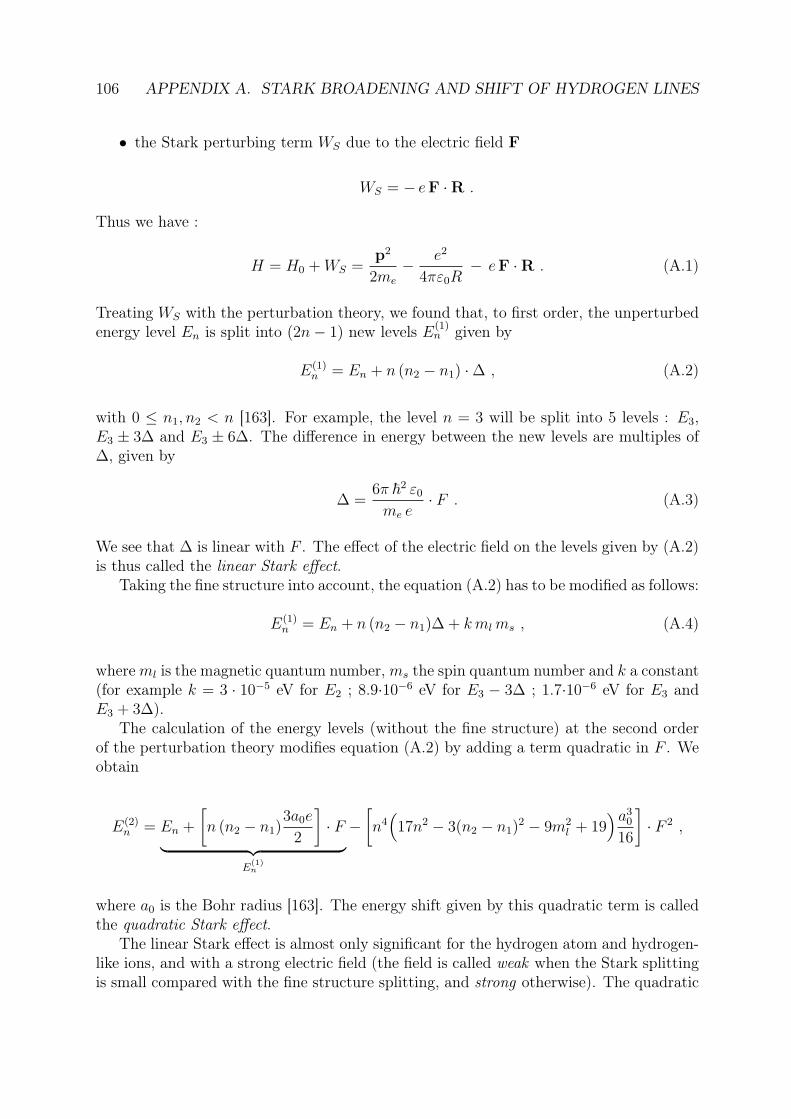
106 APPENDIX A. STARK BROADENING AND SHIFT OF HYDROGEN LINES
• the Stark perturbing term WS due to the electric field F
WS = − eF ·R .
Thus we have :
H = H0 + WS =p2
2me
− e2
4πε0R− eF ·R . (A.1)
Treating WS with the perturbation theory, we found that, to first order, the unperturbedenergy level En is split into (2n− 1) new levels E
(1)n given by
E(1)n = En + n (n2 − n1) ·∆ , (A.2)
with 0 ≤ n1, n2 < n [163]. For example, the level n = 3 will be split into 5 levels : E3,E3 ± 3∆ and E3 ± 6∆. The difference in energy between the new levels are multiples of∆, given by
∆ =6π ~2 ε0
me e· F . (A.3)
We see that ∆ is linear with F . The effect of the electric field on the levels given by (A.2)is thus called the linear Stark effect.
Taking the fine structure into account, the equation (A.2) has to be modified as follows:
E(1)n = En + n (n2 − n1)∆ + k ml ms , (A.4)
where ml is the magnetic quantum number, ms the spin quantum number and k a constant(for example k = 3 · 10−5 eV for E2 ; 8.9·10−6 eV for E3 − 3∆ ; 1.7·10−6 eV for E3 andE3 + 3∆).
The calculation of the energy levels (without the fine structure) at the second orderof the perturbation theory modifies equation (A.2) by adding a term quadratic in F . Weobtain
E(2)n = En +
[n (n2 − n1)
3a0e
2
]· F
︸ ︷︷ ︸E
(1)n
−[n4
(17n2 − 3(n2 − n1)
2 − 9m2l + 19
)a30
16
]· F 2 ,
where a0 is the Bohr radius [163]. The energy shift given by this quadratic term is calledthe quadratic Stark effect.
The linear Stark effect is almost only significant for the hydrogen atom and hydrogen-like ions, and with a strong electric field (the field is called weak when the Stark splittingis small compared with the fine structure splitting, and strong otherwise). The quadratic
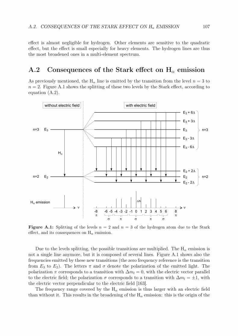
A.2. CONSEQUENCES OF THE STARK EFFECT ON Hα EMISSION 107
effect is almost negligible for hydrogen. Other elements are sensitive to the quadraticeffect, but the effect is small especially for heavy elements. The hydrogen lines are thusthe most broadened ones in a multi-element spectrum.
A.2 Consequences of the Stark effect on Hα emissionAs previously mentioned, the Hα line is emitted by the transition from the level n = 3 ton = 2. Figure A.1 shows the splitting of these two levels by the Stark effect, according toequation (A.2).
n=2
n=3
without electric field with electric field
E3
E2
E3
E2
E + 33 D
E + 63 D
E - 33 D
E - 63 D
E + 22 D
E - 22 D
Ha
n
Ha
emission
n=3
n=2
n
D/h
0 1 2 3 4-1-2-3-4
p s p
5 6 8-8 -6 -5pp
ss
Figure A.1: Splitting of the levels n = 2 and n = 3 of the hydrogen atom due to the Starkeffect, and its consequences on Hα emission.
Due to the levels splitting, the possible transitions are multiplied. The Hα emission isnot a single line anymore, but it is composed of several lines. Figure A.1 shows also thefrequencies emitted by these new transitions (the zero frequency reference is the transitionfrom E3 to E2). The letters π and σ denote the polarization of the emitted light. Thepolarization π corresponds to a transition with ∆ml = 0, with the electric vector parallelto the electric field; the polarization σ corresponds to a transition with ∆ml = ±1, withthe electric vector perpendicular to the electric field [163].
The frequency range covered by the Hα emission is thus larger with an electric fieldthan without it. This results in the broadening of the Hα emission: this is the origin of the
108 APPENDIX A. STARK BROADENING AND SHIFT OF HYDROGEN LINES
Stark broadening. If the plasma density increases, the electric field seen by the emitterwill also increase, because the charged perturbing particles will be closer. As a result, ∆will be larger according to equation (A.3). So we qualitatively see that the Hα frequencyrange, i.e. the Stark broadening of Hα, increases with density.
Taking into account the fine structure of the hydrogen atom, the Hα emission is com-posed of several lines even without electric field, because a splitting of the levels alreadyexist with F = 0. But the number of lines is also increased by the Stark effect, as shownin figure A.2 according to equation (A.4).
n=2
n=3
no field(fine structure)
weak field strong field
D5/2
P3/2 , D3/2
S1/2 , P1/2
P3/2
S1/2 , P1/2
n
0 1 2 3 4-1-2-3-4
p s p
5 6 8-8 -6 -5pp
ss
Ha
lines(strong field)
E3
E2
E + 33 D
E + 63 D
E - 33 D
E - 63 D
E + 22 D
E - 22 D
Figure A.2: Fine structure of the levels n = 2 and n = 3 of the hydrogen atom, splitting dueto the Stark effect in weak and strong field, and Hα emission in strong field.
In addition to the broadening, the Hα emission is also shifted to higher wavelengths.Equation (A.4) shows that the center of gravity of the Hα emission (E3 − E2) is shiftedfrom its position without field, due to the last term. However, this is not sufficient toexplain the measured shifts of hydrogen lines. While we can give a simple explanationfor the Stark broadening, the origin of the Stark shift of spectral lines is much morecomplicated. It involves several effects such as the quadratic Stark effect, interaction withfield gradient and emitters-electrons collisions, whereas Stark broadening involves mainlyemitter−ion collisions [107].

A.2. CONSEQUENCES OF THE STARK EFFECT ON Hα EMISSION 109
Although the origin of line shape modification by Stark effect can be simply understoodas presented here, the precise calculations of line broadening and shift require sophisticatedmodels [112–117].

110 APPENDIX A. STARK BROADENING AND SHIFT OF HYDROGEN LINES

References
[1] http://www.charmilles.ch .
[2] http://www.agie-charmilles.com .
[3] B. M. Schumacher, “After 60 years of EDM the discharge process remains stilldisputed”, J. Mater. Process. Technol., 149, 376–381 (2004).
[4] A. Anders, “Tracking down the origin of arc plasma science, I. Early pulsed andoscillating discharges”, IEEE Trans. Plasma Sci., 31(4), 1052–1059 (2003).
[5] J. Priestley, “Experiments on the circular spots made on pieces of metal by largeelectrical explosions”, in The history and present state of electricity with originalexperiments, vol. II, 3rd ed., London (1775).
[6] B. Dibner, Galvani - Volta, A controversy that led to the discovery of useful elec-tricity, CT: Burndy Library, Norwalk (1952).
[7] A. Anders, “Tracking down the origin of arc plasma science, II. Early continuousdischarges”, IEEE Trans. Plasma Sci., 31(4), 1060–1069 (2003).
[8] Handbook of vacuum arc science and technology, fundamentals and applications,edited by R. L. Boxman, D. M. Sanders and P. J. Martin, Noyes publications, ParkRidge (1995).
[9] B. R. Lazarenko, About the inversion of metal erosion and methods to fight ravageof electric contacts, WEI-Institut, Moscow (in Russian) (1943).
[10] L. H. Germer and F. E. Haworth, “Erosion of electrical contacts on make”, J. Appl.Phys., 20(11), 1085–1109 (1949).
[11] J. D. Cobine and E. E. Burger, “Analysis of electrode phenomena in the high-currentarc”, J. Appl. Phys., 26(7), 895–900 (1955).
[12] A. S. Zingerman, “The effect of thermal conductivity upon the electrical erosion ofmetals”, Sov. Phys. Tech. Phys., 1, 1945–1958 (1956).
[13] T. Sato, T. Mizutani, and K. Kawata, “Electro-discharge machine for microholedrilling”, National Technical Report, 31, 725–733 (in Japanese) (1985).
111

112 REFERENCES
[14] D. F. Dauw and B. Van Coppenolle, “On the evolution of EDM research, part 2:From fundamental research to applied research”, in Proceedings of the 11th Interna-tional Symposium for Electro Machining (ISEM-11), 133–142 (Lausanne, Switzer-land, 1995).
[15] K. Kobayashi, “The present and future developments of EDM and ECM”, in Pro-ceedings of the 11th International Symposium for Electro Machining (ISEM-11),29–47 (Lausanne, Switzerland, 1995).
[16] R. Löttgen, “EDM die-sinking - state of the art”, in Proceedings of the 12th Interna-tional Symposium for Electro Machining (ISEM-12), 341–350 (Aachen, Germany,1998).
[17] K. H. Ho and S. T. Newman, “State of the art electrical discharge machining(EDM)”, Int. J. Mach. Tools and Manufacture, 43(13), 1287–1300 (2003).
[18] K. H. Ho, S. T. Newman, S. Rahimifard, and R. D. Allen, “State of the art in wireelectrical discharge machining (WEDM)”, Int. J. Mach. Tools and Manufacture,44(12-13), 1247–1259 (2004).
[19] B. Lauwers, J.-P. Kruth, W. Liu, W. Eeraerts, B. Schacht, and P. Bleys, “Investi-gation of material removal mechanisms in EDM of composite ceramic materials”, J.Mater. Process. Technol., 149, 347–352 (2004).
[20] T. Tani, Y. Fukuzawa, N. Mohri, N. Saito, and M. Okada, “Machining phenomena inWEDM of insulating ceramics”, J. Mater. Process. Technol., 149, 124–128 (2004).
[21] H. Takezawa, H. Hamamatsu, N. Mohri, and N. Saito, “Development of micro-EDM-center with rapidly sharpened electrode”, J. Mater. Process. Technol., 149, 112–116(2004).
[22] J. Fleischer, T. Masuzawa, J. Schmidt, and M. Knoll, “New applications for micro-EDM”, J. Mater. Process. Technol., 149, 246–249 (2004).
[23] I. Beltrami, C. Joseph, R. Clavel, J.-P. Bacher, and S. Bottinelli, “Micro- and nano-electric discharge machining”, J. Mater. Process. Technol., 149, 263–265 (2004).
[24] C. Joseph, Contribution à l’accroissement des performances du processus de micro-EDM par l’utilisation d’un robot à dynamique élevée et de haute précision, PhDthesis, Ecole Polytechnique Fédérale de Lausanne, Switzerland (2005).
[25] G. Cusanelli, A. Hessler-Wyser, F. Bobard, R. Demellayer, R. Perez, andR. Flükiger, “Microstructure at submicron scale of the white layer produced byEDM technique”, J. Mater. Process. Technol., 149, 289–295 (2004).
[26] F. Klocke, D. Lung, G. Antonoglou, and D. Thomaidis, “The effects of powdersuspended dielectrics on the thermal influenced zone by electrodischarge machiningwith small discharge energies”, J. Mater. Process. Technol., 149, 191–197 (2004).

REFERENCES 113
[27] S. Das, M. Klotz, and F. Klocke, “EDM simulation: finite element-based calculationof deformation, microstructure and residual stresses”, J. Mater. Process. Technol.,142(2), 434–451 (2003).
[28] R. Perez, H. Rojas, G. Wälder, and R. Flükiger, “Theoretical modeling of energybalance in electroerosion”, J. Mater. Process. Technol., 149, 198–203 (2004).
[29] H.-P. Schulze, R. Herms, H. Juhr, W. Schätzing, and G. Wollenberg, “Comparison ofmeasured and simulated crater morphology for EDM”, J. Mater. Process. Technol.,149, 316–322 (2004).
[30] J. C. Devins, S. J. Rzad, and R. J. Schwabe, “Breakdown and prebreakdown phe-nomena in liquids”, J. Appl. Phys., 52(7), 4531–4545 (1981).
[31] P. E. Frayssines, N. Bonifaci, A. Denat, and O. Lesaint, “Streamers in liquid nitro-gen: characterization and spectroscopic determination of gaseous filament temper-ature and electron density”, J. Phys. D: Appl. Phys., 35(4), 369–377 (2002).
[32] E. O. Forster, “Progress in the understanding of electrical breakdown in condensedmatter”, J. Phys. D: Appl. Phys., 23(12), 1506–1514 (1990).
[33] E. A. Martin, “Experimental investigation of a high-energy density, high-pressurearc plasma”, J. Appl. Phys., 31(2), 255–267 (1960).
[34] P. Barmann, S. Kröll, and A. Sunesson, “Spectroscopic measurements of streamerfilaments in electric breakdown in a dielectric liquid”, J. Phys. D: Appl. Phys.,29(5), 1188–1196 (1996).
[35] S. V. Kukhlevsky, Cs. Ver, J. Kaiser, L. Kozma, L. Palladino, A. Reale, G. Tomas-setti, F. Flora, and G. Giordano, “Generation of pure, high-density metal-vaporplasma by capillary discharge”, Appl. Phys. Let., 74(19), 2779–2781 (1999).
[36] G. Wälder, “New technologies and EDM”, in Proceedings of the 12th InternationalSymposium for Electro Machining (ISEM-12), 331–340 (Aachen, Germany, 1998).
[37] F. Van Dijck, Physico-mathematical analysis of the electro discharge machining pro-cess, PhD thesis, Catholic University of Leuven, Belgium (1973).
[38] D. D. DiBitonto, P. T. Eubank, M. R. Patel, and M. A. Barrufet, “Theoreticalmodels of the electrical discharge machining process. I. A simple cathode erosionmodel”, J. Appl. Phys., 66(9), 4095–4103 (1989).
[39] M. R. Patel, M. A. Barrufet, P. T. Eubank, and D. D. DiBitonto, “Theoreticalmodels of the electrical discharge machining process. II. The anode erosion model”,J. Appl. Phys., 66(9), 4104–4111 (1989).
[40] P. T. Eubank, M. R. Patel, M. A. Barrufet, and B. Bozkurt, “Theoretical modelsof the electrical discharge machining process. III. The variable mass, cylindricalplasma model”, J. Appl. Phys., 73(11), 7900–7909 (1993).

114 REFERENCES
[41] K. Albinski, K. Musiol, A. Miernikiewicz, S. Labuz, and M. Malota, “The tem-perature of a plasma used in electrical discharge machining”, Plasma Sources Sci.Technol., 5(4), 736–742 (1996).
[42] B. W. Pillans, M. H. Evensen, H. F. Taylor, P. T. Eubank, and L. Ma, “Fiber opticdiagnostic techniques applied to electrical discharge machining sparks”, J. Appl.Phys., 91(4), 1780–1786 (2002).
[43] V. E. Fortov and I. T. Iakubov, Physics of nonideal plasma, Hemisphere, New York(1990).
[44] Transport and optical properties of nonideal plasma, edited by G. A. Kobzev,I. T. Iakubov and M. M. Popovich, Plenum Press, New York (1995).
[45] R. Redmer, “Physical properties of dense, low-temperature plasmas”, Phys. Rep.,282(2-3), 35–157 (1997).
[46] K. Günther and R. Radtke, Electric properties of weakly nonideal plasmas,Birkhäuser Verlag, Basel (1984).
[47] J. M. Meek and J. D. Craggs, Electrical breakdown of gases, Clarendon Press, Oxford(1953).
[48] L. B. Loeb, “Electrical breakdown of gases with steady or direct current impulsepotentials”, in Encyclopedia of Physics, volume XXII: Gas discharges II, edited byS. Flügge, Springer Verlag, Berlin (1956).
[49] Y. P. Raizer, Gas discharge physics, Springer-Verlag, Berlin (1991).
[50] A. E. Guile and B. Jüttner, “Basic erosion processes of oxidized and clean metalcathodes by electric arcs”, IEEE Trans. Plasma Sci., 8(3), 259–269 (1980).
[51] C. W. Kimblin, “A review of arcing phenomena in vacuum and in the transition toatmospheric pressure arcs”, IEEE Trans. Plasma Sci., 10(4), 322–330 (1982).
[52] V. I. Rakhovsky, “State of the art of physical models of vacuum arc cathode spots”,IEEE Trans. Plasma Sci., 15(5), 481–487 (1987).
[53] M. S. Benilov and A. Marotta, “A model of the cathode region of atmosphericpressure arcs”, J. Phys. D: Appl. Phys., 28(9), 1869–1882 (1995).
[54] R. L. Boxman, S. Goldsmith, and A. Greenwood, “Twenty-five years of progress invacuum arc research and utilization”, IEEE Trans. Plasma Sci., 25(6), 1174–1186(1997).
[55] I. I. Beilis, “State of the theory of vacuum arcs”, IEEE Trans. Plasma Sci., 29(5),657–670 (2001).
[56] E. Hantzsche, “Mysteries of the arc cathode spot: a retrospective glance”, IEEETrans. Plasma Sci., 31(5), 799–808 (2003).
REFERENCES 115
[57] B. Jüttner, V. F. Puchkarev, E. Hantzsche, and I. Beilis, “Cathode spots”, in Hand-book of vacuum arc science and technology, fundamentals and applications, editedby R. L. Boxman, D. M. Sanders and P. J. Martin, Noyes publications, Park Ridge(1995).
[58] A. W. Behrens, J. Ginzel, and F.-L. Bruhns, “Threshold technology and its appli-cation for gap status detection”, J. Mater. Process. Technol., 149, 310–315 (2004).
[59] P. K. Watson, W. G. Chadband, and M. Sadeghzadeh-Araghi, “The role of elec-trostatic and hydrodynamic forces in the negative-point breakdown of liquid di-electrics”, IEEE Trans. Electr. Ins., 26(4), 543–559 (1991).
[60] W. G. Chadband, “The electrical breakdown of insulating oil”, Power EngineeringJournal, , 61–67 (March 1992).
[61] R. Tobazéon, “Prebreakdown phenomena in dielectric liquids”, IEEE Trans. Diel.Electr. Ins., 1(6), 1132–1147 (1994).
[62] H. M. Jones and E. E. Kunhardt, “Development of pulsed dielectric breakdown inliquids”, J. Phys. D: Appl. Phys., 28(1), 178–188 (1995).
[63] A. Beroual, M. Zahn, A. Badent, K. Kist, A. J. Schwabe, H. Yamashita, K. Ya-mazawa, M. Danikas, W. D. Chadband, and Y. Torshin, “Propagation and structureof streamers in liquid dielectrics”, IEEE Electr. Insul. Mag., 14(2), 6–17 (1998).
[64] I. V. Lisitsyn, H. Nomiyama, S. Katsuki, and H. Akiyama, “Thermal processes in astreamer discharge in water”, IEEE Trans. Diel. Electr. Ins., 6(3), 351–356 (1999).
[65] H. M. Jones and E. E. Kunhardt, “The influence of pressure and conductivity onthe pulsed breakdown of water”, IEEE Trans. Diel. Electr. Ins., 1(6), 1016–1025(1994).
[66] O. Lesaint and G. Massala, “Positive streamer propagation in large oil gaps, Ex-perimental characterization of propagation modes”, IEEE Trans. Diel. Electr. Ins.,5(3), 360–370 (1998).
[67] G. Massala and O. Lesaint, “Positive streamer propagation in large oil gaps, Electri-cal properties of streamers”, IEEE Trans. Diel. Electr. Ins., 5(3), 371–381 (1998).
[68] A. Denat, F. Jomni, F. Aitken, and N. Bonifaci, “Thermally and electrically inducedbubbles in liquid argon and nitrogen”, IEEE Trans. Diel. Electr. Ins., 9(1), 17–22(2002).
[69] H. Yamada, T. Sato, and T. Fujiwara, “High-speed photography of prebreakdownphenomena in dielectric liquids under highly non-uniform field conditions”, J. Phys.D: Appl. Phys., 23(12), 1715–1722 (1990).
116 REFERENCES
[70] A. Beroual, C. Marteau, and R. Tobazéon, “Behavior of streamers in liquids understep voltages in point-plane geometry”, IEEE Trans. Electr. Ins., 23(6), 955–959(1988).
[71] H. Yamashita and H. Amano, “Prebreakdown phenomena in hydrocarbon liquids”,IEEE Trans. Electr. Ins., 23(4), 739–750 (1988).
[72] O. Lesaint and P. Gournay, “Initiation and propagation thresholds of positive pre-breakdown phenomena in hydrocarbon liquids”, IEEE Trans. Diel. Electr. Insul.,1(4), 702–708 (1994).
[73] Y. Nakao, H. Itoh, S. Hoshino, Y. Sakai, and H. Tagashira, “Effects of additiveson prebreakdown phenomena in n-hexane”, IEEE Trans. Diel. Electr. Ins., 1(3),383–390 (1994).
[74] T. Zinoulis, I. Argirakis, D. W. Auckland, and W. G. Chadband, “The role ofparticles in discharge initiation in liquids”, in IEEE 11th International Conferenceon Conduction and Breakdown in Dielectric Liquids (ICDL ’93), 421–425 (Baden-Dättwil, Switzerland, 1993).
[75] M. Hara, J. Suheiro, H. Maeda, and H. Nakashima, “DC pre-breakdwon phenom-ena and breakdown characteristics in the presence of conducting particles in liquidnitrogen”, IEEE Trans. Diel. Electr. Ins., 9(1), 23–30 (2002).
[76] W. G. Chadband, “From bubbles to breakdown, or vice-versa”, in IEEE 11th In-ternational Conference on Conduction and Breakdown in Dielectric Liquids (ICDL’93), 184–193 (Baden-Dättwil, Switzerland, 1993).
[77] T. Aka-Ngnui and A. Beroual, “Bubble dynamics and transition into streamers inliquid dielectrics under a high divergent electric field”, J. Phys. D: Appl. Phys.,34(9), 1408–1412 (2001).
[78] J. Qian, R. P. Joshi, J. Kolb, K. H. Schoenbach, J. Dickens, A. Neuber, M. Butcher,M. Cevallos, H. Krompholz, E. Schamiloglu, and J. Gaudet, “Microbubble-basedmodel analysis of liquid breakdown initiation by a submicrosecond pulse”, J. Appl.Phys., 97(11), 113304 (2005).
[79] S. M. Korobeinikov, A. V. Melekhov, and A. S. Besov, “Breakdown initiation inwater with the aid of bubbles”, High Temperature, 40(5), 652–659 (2002).
[80] R. Kattan, A. Denat, and O. Lesaint, “Generation, growth, and collapse of vaporbubbles in hydrocarbon liquids under a high divergent electric field”, J. Appl. Phys.,66(9), 4062–4066 (1989).
[81] A. Denat, N. Bonifaci, and M. Nur, “Spectral analysis of the light emitted by stream-ers in hydrocarbon liquids”, IEEE Trans. Diel. Electr. Ins., 5(3), 382–387 (1998).
[82] H. Akiyama, “Streamer discharges in liquids and their applications”, IEEE Trans.Diel. Electr. Ins., 7(5), 646–653 (2000).

REFERENCES 117
[83] M. Sato, T. Ohgiyama, and J. S. Clements, “Formation of chemical species andtheir effects on microorganisms using a pulsed high-voltage discharge in water”,IEEE Trans. Ind. Appl., 32(1), 106–112 (1996).
[84] M. P. Brenner, S. Hilgenfeldt, and D. Lohse, “Single-bubble sonoluminescence”, Rev.Mod. Phys., 74(2), 425–484 (2002).
[85] D. J. Flannigan and K. S. Suslick, “Plasma formation and temperature measurementduring single-bubble cavitation”, Nature, 434(7029), 52–55 (2005).
[86] J. W. Robinson, M. Ham, and A. N. Balaster, “Ultraviolet radiation from electricaldischarges in water”, J. Appl. Phys., 44(1), 72–75 (1973).
[87] A. W. DeSilva and J. D. Katsouros, “Electrical conductivity of dense copper andaluminium plasmas”, Phys. Rev. E, 57(5), 5945–5951 (1998).
[88] A. Grinenko, A. Sayapin, V. Tz. Gurovich, S. Efimov, J. Felsteiner, and Ya. E.Krasik, “Underwater electrical explosion of a Cu wire”, J. Appl. Phys., 97(2),023303 (2005).
[89] J. W. Robinson, “Measurements of plasma energy density and conductivity from 3to 120 kbar”, J. Appl. Phys., 38(1), 210–216 (1967).
[90] S. V. Kukhlevsky, J. Kaiser, O. Samek, M. Liska, and J. Erostyak, “Stark spec-troscopy measurements of electron density of ablative discharges in Teflon-(CF2)ncapillaries”, J. Phys. D: Appl. Phys., 33(9), 1090–1092 (2000).
[91] Y. Ping, I. Geltner, A. Morozov, and S. Suckewer, “Interferometric measurements ofplasma density in microcapillaries and laser sparks”, Phys. Plasmas, 9(11), 4756–4766 (2002).
[92] L. S. Caballero, H. Chuaqui, M. Favre, I. Mitchell, and E. Wyndham, “Plasma jetemission in fast-pulsed capillary discharges”, J. Appl. Phys., 98(2), 023305 (2005).
[93] C. Colon, G. Hatem, E. Verdugo, P. Ruiz, and J. Campos, “Measurement of theStark broadening and shift parameters for several ultraviolet lines of singly ionizedaluminium”, J. Appl. Phys., 73(10), 4752–4758 (1993).
[94] M. A. Hafez, M. A. Khedr, F. F. Elaksher, and Y. E. Gamal, “Characteristics ofCu plasma produced by a laser interaction with a solid target”, Plasma Sources Sci.Technol., 12(2), 185–198 (2003).
[95] Y. Zhang, L. Li, and G. Zhang, “Spectroscopic measurements of plasma inside thekeyhole in deep penetration laser welding”, J. Phys. D: Appl. Phys., 38(5), 703–710(2005).
[96] V. A. Alekseev and I. T. Iakubov, “Non-ideal plasmas of metal vapours”, Phys. Rep.,96(1), 1–69 (1983).
118 REFERENCES
[97] K. Terashima, L. Howald, H. Haefke, and H.-J. Güntherodt, “Development ofa mesoscale/nanoscale plasma generator”, Thin Solid Films, 281-282, 634–636(1996).
[98] Y. Hirata, M. Fukushima, T. Sano, K. Ozaki, and T. Ohji, “Micro-arc dischargephenomena”, Vacuum, 59(1), 142–151 (2000).
[99] T. Ito, T. Izaki, and K. Terashima, “Development of plasma chip”, Surf. Coat.Technol., 133-134, 497–500 (2000).
[100] C. Penache, M. Miclea, A. Bräuning-Demian, O. Hohn, S. Schlössler, T. Jahnke,K. Niemax, and H. Schmidt-Böcking, “Characterization of a high-pressure microdis-charge using diode laser atomic absorption spectroscopy”, Plasma Sources Sci. Tech-nol., 11(4), 476–483 (2002).
[101] M. Miclea, K. Kunze, J. Franzke, and K. Niemax, “Plasmas for lab-on-the-chipapplications”, Spectrochim. Acta B, 57(10), 1585–1592 (2002).
[102] R. Longwitz, Study of gas ionization in a glow discharge and development of a microgas ionizer for gas detection and analysis, PhD thesis, Ecole Polytechnique Fédéralede Lausanne, Switzerland (2004).
[103] T. Ito, T. Izaki, and K. Terashima, “Application of microscale plasma to materialprocessing”, Thin Solid Films, 386(2), 300–304 (2001).
[104] O. B. Postel and M. A. Cappelli, “Parametric study of the vacuum ultraviolet emis-sion and electrical characteristics of a He-Xe microdischarge”, J. Appl. Phys., 89(9),4719–4726 (2001).
[105] K. H. Becker, K. H. Schoenbach, and J. G. Eden, “Microplasmas and applications”,J. Phys. D: Appl. Phys., 39(3), R55–R70 (2006).
[106] G. Sémon, Guide pratique d’usinage par étincelage, Ateliers des Charmilles S.A.,Genève (1977).
[107] H. R. Griem, Principles of Plasma Spectroscopy, University Press, Cambridge(1997).
[108] R. Rompe and M. Steenbeck, Progress in plasmas and gas electronics, volume 1,Akademie-Verlag, Berlin (1975).
[109] T. Fujimoto, Plasma Spectroscopy, Clarendon Press, Oxford (2004).
[110] K. Fu, M. Jogwich, M. Knebel, and K. Wiesemann, “Atomic transition probabilitiesand lifetimes for the Cu I system”, At. Data Nucl. Data Tables, 61(1), 1–30 (1995).
[111] H. R. Griem, Spectral line broadening by plasmas, Academic, New York (1974).
REFERENCES 119
[112] M. A. Gigosos and V. Cardenoso, “New plasma diagnosis tables of hydrogen Starkbroadening including ion dynamics”, J. Phys. B: At. Mol. Opt. Phys., 29(20),4795–4838 (1996).
[113] S. Böddeker, S. Günter, A. Könies, L. Hitzschke, and H.-J. Kunze, “Shift and widthof the H alpha line of hydrogen in dense plasmas”, Phys. Rev. E, 47(4), 2785–2791(1993).
[114] W. Olchawa, “Computer simulations of hydrogen spectral line shapes in dense plas-mas”, J. Quant. Spectrosc. Radiat. Transfer, 74(4), 417–429 (2002).
[115] S. A. Flih, E. Oks, and Y. Vitel, “Comparison of the Stark widths and shifts of theH-alpha line measured in a flash tube plasma with theoretical results”, J. Phys. B:At. Mol. Opt. Phys., 36(2), 283–296 (2003).
[116] S. Günter and A. Könies, “Shifts and asymmetry parameters of hydrogen Balmerlines in dense plasmas”, Phys. Rev. E, 55(1), 907–911 (1997).
[117] A. Escarguel, E. Oks, J. Richou, and D. Volodko, “Highly nonlinear, sign-varyingshift of hydrogen spectral lines in dense plasmas”, Phys. Rev. E, 62(2), 2667–2671(2000).
[118] W. Weibull, “A statistical distribution function of wide applicability”, J. Appl.Mech., 18, 293–297 (1951).
[119] C. J. Frei, “Weibull statistical analysis of dielectric breakdown in n-hexane”, IEEETrans. on Electr. Insul., 20(2), 303–307 (1985).
[120] C. J. Frei, L. He, and K. Müller, “Implications from the influence of electrohydrody-namic motion on breakdown with respect to the discharge mechanism in dielectricliquids”, IEEE Trans. on Electr. Insul., 24(2), 169–174 (1989).
[121] A. Karden, Der Entladekanal - Was passiert wirklich bei der Funkenerosion?, BerichtNr. 272-1/00, Laboratorium für Werkzeugmaschinen und Betriebslehre, Rheinisch-Westfälischen Technischen Hochschule, Aachen (2001).
[122] E. Gidalevich and R. L. Boxman, “Sub- and supersonic expansion of an arc channelin liquid”, J. Phys. D: Appl. Phys., 39(4), 652–659 (2006).
[123] B. Revaz, G. Witz, and R. Flükiger, “Properties of the plasma channel in liquiddischarges inferred from cathode local temperature measurements”, J. Appl. Phys.,98(11), 113305 (2005).
[124] P. C. Pandey and S. T. Jilani, “Plasma channel growth and the resolidified layer inEDM”, Precis. Eng., 8(2), 104–110 (1986).
[125] G. Cusanelli, PhD thesis, Université de Genève, Switzerland (2004).

120 REFERENCES
[126] A. E. Berkowitz and J. L. Walter, “Spark erosion: a method for producing rapidlyquenched fine powders”, J. Mater. Res., 2(2), 277–288 (1987).
[127] J. Carrey, H. B. Radousky, and A. E. Berkowitz, “Spark-eroded particles: Influenceof processing parameters”, J. Appl. Phys., 95(3), 823–829 (2004).
[128] C. E. Moore, A multiplet table of astrophysical interest, U.S. Department of Com-merce, National Bureau of Standards, Washington (1959).
[129] PLASUS SpecLine Software, http://www.plasus.de .
[130] J. Reader, C. H. Corliss, W. L. Wiese, and G. A. Martin, Wavelengths and transitionprobabilities for atoms and atomic ions, U.S. Department of Commerce, NationalBureau of Standards, Washington (1980).
[131] R. W. B. Pearse and A. G. Gaydon, The identification of molecular spectra, Wiley,New York (1950).
[132] NIST Atomic Spectra Database, http://www.physics.nist.gov/PhysRefData/ASD .
[133] D. J. Heading, G. R. Bennett, J. S. Wark, and R. W. Lee, “Novel plasma source fordense plasma effects”, Phys. Rev. Lett., 74(18), 3616–3619 (1995).
[134] Y. Vitel, M. El Bezzari, T. V. Gavrilova, M. Skowronek, L. G. D’yachkov, andY. K. Kurilenkov, “On dense hydrogen and noble gases plasma spectra”, Physica B,228(1-2), 161–165 (1996).
[135] A. Escarguel, B. Ferhat, A. Lesage, and J. Richou, “A single laser spark in aqueousmedium”, J. Quant. Spectrosc. Radiat. Transfer, 64(4), 353–361 (2000).
[136] B. Revaz, J. Emery, G. Witz, R. Flükiger, R. Perez, J. Carron, and M. Rappaz,“Local temperature response to pulsed discharges in electronic discharge machining(EDM) environment”, IEEE Trans. Plasma Sci., 33(3), 1066–1071 (2005).
[137] H. R. Griem, “Validity of local thermal equilibrium in plasma spectroscopy”, Phys.Rev., 131(3), 1170–1176 (1963).
[138] K. Song, H. Cha, J. Lee, and Y.-I. Lee, “Investigation of the line-broadening mech-anism for laser-induced copper plasma by time-resolved laser-induced breakdownspectroscopy”, Microchem. J., 63(1), 53–60 (1999).
[139] J. D. Huba, NRL Plasma formulary, Naval Research Laboratory, Washington(2004).
[140] M. M. Litvak and D. F. Edwards, “Spectroscopic studies of laser-produced hydrogenplasma”, IEEE J. Quant. Electronics, 2(9), 486–492 (1966).
[141] W. L. Wiese, D. E. Kelleher, and D. R. Paquette, “Detailed study of the Starkbroadening of Balmer lines in a high-density plasma”, Phys. Rev. A, 6(3), 1132–1153 (1972).

REFERENCES 121
[142] Y. Vitel, “Experimental study of Hα broadening and shift in dense argon plasmas”,J. Phys. B: At. Mol. Phys., 20(10), 2327–2337 (1987).
[143] C. Parigger, J. W. L. Lewis, and D. Plemmons, “Electron number density andtemperature mesurement in a laser-induced hydrogen plasma”, J. Quant. Spectrosc.Radiat. Transfer, 53(3), 249–255 (1995).
[144] Y. Vitel, T. V. Gavrilova, L. G. D’yachkov, and Y. K. Kurilenkov, “Spectra of densepure hydrogen plasma in Balmer area”, J. Quant. Spectrosc. Radiat. Transfer, 83(3-4), 387–405 (2004).
[145] A. Cohn, P. Bakshi, and G. Kalman, “Linear Stark effect due to resonant interactionsof static and dynamic fields”, Phys. Rev. Lett., 29(6), 324–327 (1972).
[146] C. C. Gallagher and M. A. Levine, “Balmer-line anomalies in a turbulent plasma”,Phys. Rev. Lett., 30(19), 897–900 (1973).
[147] W. R. Rutgers and H. W. Kalfsbeek, “Calculations and measurements of the dy-namic Stark effect in hydrogen”, Z. Naturforsch., 30(a), 739–749 (1975).
[148] A. I. Zhuzhunashvili and E. A. Oks, “Technique of optical polarization measurementsof plasma Langmuir turbulence spectrum”, Sov. Phys. JETP, 46(6), 1122–1129(1977).
[149] K. H. Finken, R. Buchwald, G. Bertschinger, and H.-J. Kunze, “Investigation of theH alpha line in dense plasmas”, Phys. Rev. A, 21(1), 200–206 (1980).
[150] V. P. Gavrilenko and E. A. Oks, “Intra-Stark spectroscopy of Coulomb radiatorsin a plasma with quasimonochromatic electric field”, Sov. J. Plasma Phys., 13(1),22–28 (1980).
[151] G. Kalman and P. Bakshi, “Microfield effects: strongly coupled plasmas”, J. Quant.Spectrosc. Radiat. Transfer, 44(1), 1–9 (1990).
[152] P. Bakshi and G. Kalman, “Hydrogenic spectroscopy for various unusual plasmas”,J. Quant. Spectrosc. Radiat. Transfer, 44(1), 93–100 (1990).
[153] E. A. Oks, S. Böddeker, and H.-J. Kunze, “Spectroscopy of atomic hydrogen indense plasmas in the presence of dynamic fields: Intra-Stark spectroscopy”, Phys.Rev. A, 44(12), 8338–8347 (1991).
[154] D. R. Inglis and E. Teller, “Ionic depression of series limits in one-electron spectra”,Astrophys. J., 90, 439–448 (1939).
[155] C.-R. Vidal, “Determination of electron density from line merging”, J. Quant. Spec-trosc. Radiat. Transfer, 6(4), 461–477 (1966).
[156] K. M. Roussel and R. F. O’Connell, “A comparison between Debye-Hückel screeningand the stark effect on the determination of the last observable spectral line from ahydrogen-like plasma”, Phys. Lett. A, 51(4), 244–246 (1975).
122 REFERENCES
[157] N. Konjevic, “Plasma broadening and shifting of non-hydrogenic spectral lines:present status and applications”, Phys. Rep., 316(6), 339–401 (1999).
[158] N. Konjevic and W. L. Wiese, “Experimental Stark widths and shifts for spectrallines of neutral and ionized atoms”, J. Phys. Chem. Ref. Data, 19(6), 1307–1385(1990).
[159] M. R. Zaghloul, M. A. Bourham, and J. M. Doster, “A simple formulation andsolution strategy of the Saha equation for ideal and nonideal plasmas”, J. Phys. D:Appl. Phys., 33(8), 977–984 (2000).
[160] L. Spitzer and R. Härm, “Transport phenomena in a completely ionized gas”, Phys.Rev., 89(5), 977–981 (1953).
[161] J. W. Mackersie, I. V. Timoshkin, and S. J. MacGregor, “Generation of high-powerultrasound by spark discharges in water”, IEEE Trans. Plasma Sci., 33(5), 1715–1724 (2005).
[162] C. Cohen-Tannoudji, B. Diu, and F. Laloë, Mécanique quantique, Hermann, Paris(1973).
[163] H. G. Kuhn, Atomic Spectra, Longmans, London (1962).

Acknowledgments
This last chapter is undoubtedly the most pleasant one to write. It would have beenimpossible to complete this thesis without the help of many people. Since they all under-stand my mother tongue, I wish to warmly thank them en français dans le texte.
Mes remerciements vont naturellement tout d’abord au Dr Christoph Hollenstein, di-recteur du groupe des plasmas industriels du CRPP et directeur de ma thèse, sans qui rienn’aurait été possible et grâce à qui j’ai beaucoup appris. Travailler sous sa supervision,et ainsi pouvoir profiter de sa grande expérience et de son sens aigu de la physique, aété un réel plaisir pendant ces cinq ans. Ses qualités scientifiques mais aussi humainesont largement contribué au succès de mon travail de thèse. Merci énormément, Christoph !
Je remercie très sincèrement les personnes de Charmilles Technologies qui ont col-laboré à ce projet, spécialement le Dr Georg Wälder qui m’a suivi pendant tout ce tra-vail et qui m’a fait le plaisir d’être membre de mon jury. Un grand merci également àRené Demellayer et au Dr Roberto Perez, pour avoir partagé leur grande connaissancede l’électro-érosion et pour leurs précieux conseils. Merci à vous tous pour votre soutientechnique et scientifique, ainsi que pour votre enthousiasme face à mon travail.
Je tiens aussi à remercier les Drs Ivano Beltrami et Cédric Joseph ainsi que MarcoBoccadoro de Agie, pour les discussions fructueuses que j’ai eues avec eux et leur intérêtpour mon projet.
Je remercie sincèrement MM. les professeurs Michel Rappaz et Jörg Winter qui ontaccepté de faire partie de mon jury de thèse, ainsi que M. le professeur Robert Schallerqui l’a présidé.
Si le directeur d’un groupe de recherches est essentiel, ses autres membres ne le sontpas moins. Un très très très grand MERCI au Dr Jean-Luc Dorier, qui a toujours suécouter et trouver des réponses à mes questions tant scientifiques que techniques. MerciJean-Luc de m’avoir fait profiter de tes impressionnantes connaissances, et merci de nejamais être à court de gentillesse et de bonne humeur ! Je remercie également les DrsAlan Howling et Laurent Sansonnens pour leur disponibilité et leurs conseils toujourspertinents. Je suis particulièrement reconnaissant envers Alan qui a relu et corrigé cemanuscrit, et qui a ainsi rendu le texte un peu plus oxfordien.
Un grand merci aux doctorants du groupe, Samantha Pavon, Lukas Derendinger,Hannes Schmidt et Benjamin Strahm, mais aussi à il Dottore Raffaello Sobbia, pour avoircontribué à l’excellente ambiance de travail. Evidemment, un merci tout particulier à
123
124 ACKNOWLEDGMENTS
Alban Sublet, ambassadeur de Haute-Savoie en Suisse, qui est devenu au fil de ces annéesbien plus qu’un simple collègue de travail. Merci Alban, collègue physicien, joggeur,fondeur, skieur, vététiste, randonneur, cinéaste, cinéphile, photographe, mélomane, etj’en oublie. T’es un jeune qui n’en veut, moi je dis chapeau.
Je tiens également à remercier les anciens doctorants du groupe, tout spécialementles Drs Thierry Delachaux et Malko Gindrat. Merci les gars pour les très nombreuxmoments de rire passés ensemble, sans vous ce n’est plus pareil... Merci Thierry pourles kilomètres courus en ta compagnie, en particulier ces 26.2 miles de souffrance entreHopkinton et Boston un jour trop chaud d’avril. Et merci Malko, mon voisin de bureaupendant plusieurs années, de m’avoir transmis un peu de ta connaissance inépuisable del’informatique.
Mes remerciements vont bien sûr également aux différents services techniques duCRPP. Merci aux mécaniciens, électriciens, électroniciens, au service du vide et au serviceinformatique, pour les “p’tits boulots” occasionnels sans lesquels on n’avance pas au labo.Un très grand merci au secrétariat pour toutes les tâches administratives, avec mentionspéciale pour Edith Grüter. Merci de tout mon coeur Edith, pour tout et surtout pourtout le reste !
Je tiens aussi à saluer Alexandre Blais, de l’université d’Ottawa certes, mais Québé-cois avant tout. Merci Alex de ton passage en Suisse, et merci mille fois de m’avoir faitdécouvrir les richesses de ta belle province. J’ai eu bin d’s’fonne avec toé, mon go !
Enfin, je remercie infiniment tous les membres de ma famille, les personnes les plusimportantes de ma vie, pour leur soutien tout au long de ces années. Merci à la nouvellegénération, Arthur, Gaspard, Anna, Elise et Camille, pour tout le bonheur que vousme transmettez. Merci à mes indispensables soeurs, Véronique, Noémie et Sarah, maiscomment diable vivrais-je sans vous ?!? Merci à vous d’avoir choisi Françoise, Antoine etStephan, je n’aurais pu faire meilleurs choix... Et un merci incommensurable à Maman età Papa, pour m’avoir soutenu de toutes les manières possibles et m’avoir donné la chancede toujours pouvoir choisir et réaliser ce que j’ai eu envie de faire. Vous m’avez en plusdonné l’amour de la Science, merci de m’avoir fait ce si beau cadeau...
Antoine
Curriculum Vitae
Antoine DESCOEUDRES
Né le 2 février 1978 à Lausanne (VD),de nationalité suisse et originaire de La Sagne (NE).
FORMATION
2002 - 2006 Thèse de doctorateffectuée dans le groupe des plasmas industriels,Centre de Recherches en Physique des Plasmas (CRPP),Ecole Polytechnique Fédérale de Lausanne (EPFL).Assistant pour divers cours de Physique générale.
1996 - 2001 Diplôme d’ingénieur physicien, EPFLTravail de diplôme effectué au CRPP.
1993 - 1996 Baccalauréat ès lettres (mention latin-mathématiques) etCertificat de maturité - type A (latin-grec)Gymnase cantonal du Bugnon, Lausanne.
PUBLICATIONS
A. Descoeudres, L. Sansonnens and C. Hollenstein, “Attachment-induced ionization insta-bility in electronegative capacitive RF discharges”, Plasma Sources Sci. Technol., 12(2),152-157 (2003).
A. Descoeudres, C. Hollenstein, R. Demellayer and G. Wälder, “Optical emission spec-troscopy of electrical discharge machining plasma”, J. Phys. D: Appl. Phys., 37(6),875-882 (2004).
A. Descoeudres, C. Hollenstein, R. Demellayer and G. Wälder, “Optical emission spec-troscopy of electrical discharge machining plasma”, 14th International Symposium for Elec-tromachining (ISEM XIV), April 2004, Edinburgh, Scotland.J. Mater. Process. Technol., 149, 184-190 (2004).
A. Descoeudres, C. Hollenstein, G. Wälder and R. Perez, “Time-resolved imaging andspatially-resolved spectroscopy of electrical discharge machining plasma”, J. Phys. D:Appl. Phys., 38(22), 4066-4073 (2005).