characterization of domains of fractional powers of ... · 282 chen and triggiani where e,, denotes...

JOURNAL OF DIFFERENTIAL EQUATIONS 88, 279-293 (1990)

Characterization of Domains of Fractional Powers of Certain Operators Arising in Elastic Systems,

and Applications

%IJPING CHEN *

Department of Mathematics, Zhejiang University, Hongzhou, China

AND

ROBERTO TRIGGIANI’

Department of Applied Mathematics, Thornton Hall, University of Virginia, Charlottesville, Virginia 22903

Received August 23, 1989

1. INTRODUCTION: STATEMENT OF MAIN RESULT

This note is a continuation of our previous efforts [CTl, CT41 on the second-order abstract equation

R+Bi+Ax=O, on X,

or l~~=~~A yBI ICI on E=z?~(A*/~)xX, (“l)

with X a Hilbert space, where A, the elastic operator, and B, the damping operator, are closed operators in X, with dense domains Q(A) and 9(B), respectively. Moreover, A is throughout assumed to be self-adjoint and strictly positive. Stimulated by two conjectures raised in [CRl] (the most general of which referred to the case LX = f described below), we have already studied the operators &” and SB,, defined respectively by

(1.2)

where p > 0 is a constant, and have obtained a number of results. A subset of these, relevant to the present note, is as follows. Let B be self-adjoint on X, and let B be comparable to A*, 0 < a < 1, in the sense

plAa<B<p2Aa forsome O<p,ep,<oo. (1.3)

* Research partially supported by the National Science Foundation of China. t Research partially supported by the National Science Foundation under Grant DMS-87-

96320 and by the Air Force Offke of Scientific Research under Grant AFOSR-87-0321.

279 0022-0396190 S3.00

Copyright 0 ,990 by Academic Press, Inc. All rights of reproduction in any form reserved.

280 CHEN AND TRIGGIANI

Then, &B is the generator of a S.C. contraction semigroup on E which, if +<a < 1, is moreover analytic on E, [CTl, CT2]; while, if O< z < f, is Gevrey class of order 6 > 1/2a, hence differentiable on E for all t > 0, but generally not analytic here [CT3]. The assumption that B be self-adjoint may be removed and replaced with the assumption that (1.3) reads now with Re(Bx, x) in place of (Bx, x) and that, moreover, 1 Im( Bx, x)1 < KRe(B.u, x), see [CT3, Remark 1.11. Other results, requiring conditions on B*, are also available [CT2, p. 21; CT43; see also [Hl, H2, FOl].

These results imply that elastic systems with a “sufficiently strong” damping as expressed by (1.3), have a parabolic-like behavior. This opens the door to a whole series of new questions. In the present note we specialize to B = pA”, p > 0, 4 d CI Q 1, and study the domains of fractional powers 5?( ( --A,,)‘), 0 < 8 < 1, of the operator ( -J%‘~,) on E, which is well defined. Besides being of interest in itself, this issue has a number of important consequences. A few are taken up in this note for purposes of ‘illustration. Others are considered in separate papers [T2; LTl, Sect. 3; LT2, Sect. 61. Our main result in this note is a characterization of 9( ( -J&)‘) in terms of domains of fractional powers of A.

THEOREM 1.1. Consider the operator JdPx: ~(Jz$,) + E in (1.2) with p>O, ida<l.

(i) Let 0<6<+. Then

9((-dp,)e)=~(A’~*+e(‘-z’)X9(Aze). (1.4)

(ii) Let i6 0 < 1. Then

W( -J$,J8) = iI I

; EE:xE~(A 1j2+0(1-9; yE~(AZ-1/2+e(1--i),

AL-‘x+py~9(Aae) . 1

(1.5)

Note that for a = 4, the third requirement in (1.5) is automatically satislied. The proof of Theorem 1.1, which shows the exact form of the map ( -JZ$,)’ from its domain onto E, and of its inverse ( -JZ$,.)-~ from E onto 9(( -JZ$,,)‘), is given in Sections 2 and 3. We then consider a few applications of Theorem 1.1. In Section 4, we establish that the operator JJ?” in (1.2) generates, under certain conditions, an S.C. analytic semigroup on E without any hypothesis on B*, unlike the results referred to below (1.3). In Section 5, we give one illustration of maximal regularity of the solutions to the corresponding nonhomogeneous problem (Eq. (5.1) below with f~ L,(O, T; X)). Other illustrations are possible, where f may be “a point load” (a-function or its derivative, concentrated at an interior point of a

DOMAINSOFFRACTIONALPOWRS 281

bounded domain a, where the “concrete” partial differential equation corresponding to (5.1) is defined). Indeed, Theorem 1.1 can be used also in the case of elastic systems described by a suitable partial differential equation defined in an open bounded domain 52 c R” with nonhomogeneous term acting on the boundary dQ of Q. These questions are examined in [T2; LTl, Sect. 3; LT2, Sect. 61.

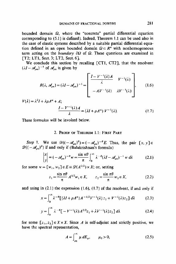
We conclude this section by recalling [CTl, CT2], that the resolvent (AZ- alp,) -’ of zZ,, is given by

R(A, a$,) = (AZ- a$,)-’ = 9 (1.6) -AV-‘(A) IIf-’

V(A) = 12Z+ IpA” + A;

I- v;‘(A)A = (AZ+ PA”) V-‘(n). (1.7)

These formulas will be invoked below.

2. PROOF OF THEOREM 1.1: FIRST PART

Step 1. We use 9( ( -JZ$,)“) = ( -&Pcl)-BE. Thus, the pair [x, y] E 9(( --dP,)‘) if and only if (Balakrishnan’s formula)

for some )t’= [wr, wa] EEc~(A”*)x X, or, setting

sin 7~0 A”*W EX

sin ne z, =- 1 3

n z* = - w* E x,

n (2.2)

and using in (2.1) the expression (1.6), (1.7) of the resolvent, if and only if

x= s ml-“[(1Z+pA”)A-L~2V-1(17.)~I+ V-‘(J)z,] dl (2.3) 0

y= a I-‘[ - I/-‘(&d”*Z, +~V-‘(~)z2] d3, (2.4)

for some [zi, z2] E XxX. Since A is self-adjoint and strictly positive, we have the spectral representation,

A= =pdEP, s clo=+o, (2.5) PO


where E,, denotes the usual family of orthogonal projections. Recalling (1.7), we then rewrite (2.3) and (2.4), respectively, as

Note that dE, is finite measure. Since Fubini’s theorem applies on a smooth set dense on Xx X, we may interchange the order of integrations in (2.6), (2.7): we set

(2.8)

and obtain for all [z,, z2] E Xx X

i

,~=A-1~2g,(A)~,+pA~-1~2g2(A)~,+g2(Aji2; (2.9) y= -A’:*

‘!Y,(A)i, +g,(Ab,. (2.10)

Step 2.

LEMMA 2.1. We have (explicit dependence on p, tl, 8 will be suppressed)

(i) T, = TL.pro = A”g,(A ) is an isomorphism on X, (2.11) (ii) T, = T2,P;r0 - A B+z-e’g2(A) is an isomorphism on X. (2.12)

T, and T, are strictly positive, self-aa’joint operators which commute with any analytic function of A (a fact which we shall use freely below).

The proof of this lemma is given at the end.

Step 3. Using the isomorphisms of Lemma 2.1, we rewrite (2.11) and (2.12) as

i

x~A~~~~--~T,~,+~A-‘~~+~~-~T~~~+A-@-~+~~T~~,; (2.13) I’= -,41,2-0-Y+& Tzi, + A-“‘T,Z2; (2.14)

{

X=A-1’2+eb1,T3Z, +A-Z+6bl,T _ . 2L27 (2.15)

?I= _A’~*-“+8(“~‘)Tzz,+A-JLBTIZ2; (2.16)

after introducing the positive self-adjoint operator,

T, = T3,p.e = A”’ ~ 2b’T, + pT2 : isomorphism on X (2.17)

for $< CI as assumed. We note that all exponents of A in (2.15), (2.16) are nonpositive for i < 016 1; 0 < 0 < 1. So far we have shown that a pair

DOMAINS OF FRACTIONAL POWERS 283

[x, y] ~g(( -z$,)‘) if and only if it can be written as in (2.13), (2.14), or else as in (2.15), (2.16), for a suitable [z,, zz] EXX X.

Step 4. We draw some consequences for x, y as in (2.13)/(2.15), or (2.16); i.e., for [x, ~1 E g(( --LX&)‘). For any [z,, z2] E Xx X, we have

~-I’2+B(a-11)T3Z~E~(Ali2+e~l-“‘), A-1+e(~-lI)T2Z2E~(AJL+e(l-bl)),

(2.18)

and since f+O(l-a)=(a+O-a@)+($-a), where $--ado, we obtain by (2.18) used in (2.15) that

XE9(A l/Z+e(l--a) 1. (2.19)

Moreover, for any [zl, z2] E Xx X, we have

~li2-a+~~.~1)T2Z,E~(AOL~l/2+B(I--a~), A-“0T1z2EG@A~0). (2.20)

But for a 2 4 as assumed

Thus, by (2.20t(2.22) used in (2.16), we obtain

i WA’?, if o<e<i (2.23)

Y E 9(A’- 1/2+.9(1-m) ), if ;<e<i. (2.24)

Finally, we return to (2.13), (2.14): We apply pAa-’ to (2.14) and add up the result to (2.13). After a cancellation of the term pA-1’2fue-eT2~,, we obtain

x+pA U-iy=A-~,‘-CZeT z I I (E S?(A”‘2+ue)

+ A-e-r+aeT2z2 (E WA e+a-ae))

+PA a-l-ae T7 1-2 (E WA ae+‘-a))9 (2.25)

or, since 8+a-a0~c&-a+ 1, as well as $+aeaa8-a+ 1, for ;<a; 8< 1, we have from (2.25),

x+pA r-lyE~(A”e+l--;I), or A I-“x+py~L@(A”~) (2.26)

an “interaction condition.” Note that for x as in (2.19) and y as in (2.23) for 0 < i, the interaction condition (2.26) is automatically satisfied, since (2.19) readily implies ALezx~ LS(A- 1/2+e-eor+a)~L2(Aea) for f3<;, aaf. We have shown

284 C‘HEN AND TRIGGIANI

LEMMA 2.2. Ler [s, ~11 EP(( -s&J”) so that (2.14), (2.15), and (2.16 hold. Then I and y satisj.i* (2.19), (2.23), (2.24), and (2.26); i.e.,

o<e+: ~((-.~,,)“)cy(A’.l+fj(’ l))xp(A”f’) (2.27

$QB<l: Q’(( -dQqc -; :sEGyA’ 2+H”-x’); ii I

J?ES’(A I~I;:+H~l~n);AI-Z.u+p~,E~(AZH) . 1

(2.28)

Step 5. We next invert the transformation ( -s$,))~: X x x 3 cz, 3 z2 ] + [x, y] defined by (2.15), (2.16) in an explicit manner.

Case. 0 < 6 < +.

Here we use only the regularity properties (2.19) for x and (2.23) for y. We apply A 1”2+B-reTl to (2.15) and A’!2-z+eaT2 to (2.16) (both being legal operations; f < c(), subtract the second identity from the first and obtain after cancellation of A’!’ ~ ‘T, T, z2,

A”2+e-oaT x-A’:2-“+~“T2y=T3T,;,+AlI~2a)(1-~’T:Z, I

= T,z,, (2.29)

where we have introduced the positive self-adjoint operator

T4 = T4,Pire = T, T3 + A” - “)” ~ “‘T:: isomorphism on X (2.30)

(since the exponent of A is nonpositive , $ < a), which commutes with any analytic function of A. Thus, from (2.29) we obtain

z = T-I/,1)2+&& T,x- T-~A~.‘:-LT+~Z I 4 4 T2 Y. (2.31)

Inserting (2.31) into (2.16), after the latter has been pre-multiplied by A”, yields

z2 - _A’2”~‘“e~1;2)Al;2+B~aHT2TqI.~+ T,-l

x(1-A ~2cl~~)(~-1/21+l/2--~~~T~)AoL~y~ (2.32)

Equation (2.32) has been written in a form more complicated than necessary to evidence at once that it is well defined for x as in (2.19) and y as in (2.23) ((201.1)(0-- f) < 0, f- tl<O under our present assumptions). Thus, given x as in (2.19) and y as in (2.23), then (2.31), (2.32) produce the pair [z,, zz] EXX A’ which is mapped into [x, y] by ( - JZ’~,) -‘. We have proved

DOMAINSOFFRACTIONAL POWERS 285

LEMMA 2.3. Let 0~ 8 <i. Then

9(A “2+ec’-“‘)~9(Aae)c~((-dp,)o). (2.33)

Step 6, We now invert the transformation ( -szZ~,)-~ defined by (2.13)/(2.15) and (2.16) for $<O< 1. Thus we shall now use only the regularity properties (2.19) for x, (2.24) for y, as well as the “interaction” condition (2.26). We apply A’i2ce~ozT2 to (2.15), Aa-‘12C8(1-‘JL)T3 to (2.16), add the resulting identities, and obtain after a cancellation of T,T,z,,

or, after recalling the definition (2.17) of T3

Aa-ii*-ecr+eT2(Ai-*x+PY)+Al-1/2+2e~30LeT,I!

=A 1/2-UT2 2z2+A('~L'2)(1-2e)T1T3Z2, (2.35)

or, after using the interaction property (2.26) and the definition (2.30) of T,,

A(“-1/*)(1-*e)AZeT2(A’~*x+py)+A(”-i/2~~’-*e)Ae(l-jl)T, v

=A(cL-w-*e)T4z2 (2.36)

Note that all quantities are well defined under present assumptions ((a-$)(l-228)cO and a-i+O-a(?=(~-$)+&l-a), with (a-f)20 so that (2.24) yields y~9(A~“-“). Thus (2.36) yields

z2= T,-‘AaeT2(A1-“x+py)+ T,-‘A”‘-“T,y. (2.37)

We next insert (2.37) into (2.15), after the latter has been premultiplied by A’i2+epe”, to obtain

z1 = T;lAl/*+e- “x- T-1A1!2-“T2T,-1[Ao”T2(A’~a~+py)] 3

- T;‘A w-UT2 T,- IA@' -oI)TL y. (2.38)

Note that all terms in (2.37), (2.38) are well defined for x and )’ satisfying (2.19), (2.24), (2.26). Thus, given such a pair [x, ~1, then (2.37), (2.38) produce the pair [z,, z2] E Xx X which is mapped into [x, JJ] by ( - s$,) -‘. We have proved

LEMMA 2.4. Let i < 0 < 1. Then

c W( -J$de). (2.39)

286 CHEN AND TRIGCiIANI

Then Lemmas 2.2, 2.3. 2.4 prove Theorem 1.1, as soon as we prove Lemma 2.1.

3. COMPLETION OF THE PROOF OF THEOREM 1. I: PROOF OF LEMMA 2.1

Proof of (2.11). We shall show that for each 0 < 8 < 1, there exist two . . postttve constants c,~ and CL0 (depending not only on 8, but also possibly on p0 > 0, p, etc.) such that

0 < c,e d P”%,(P) Q c,e < m, Vp2p()>O. (3.1

Indeed, in the integral, see (2.8)

(3.2

we divide by p both numerator and denominator, introduce a new variable 0 = A/& and obtain

(3.3)

If now 0 < p0 <p d 1, we drop the second integral on the right of (3.3), replace 0 with ,u- Ii2 in the denominator of the first integral in (3.3) and obtain

p*,2KI(~)Bf~“I~2+~blll~,2 P

(1--LizJ(z-e)

+ 1 2 c(pa-“‘2)2 (1 +p)+ 1](2-8)

after majorizing p’ - ‘12 by 1 in the denominator, or

(3.4)

2sr- 1

P ‘%- ‘~2)ePef2g,(/4 2 (2 +p;H2 _ (3)’ O<p,GpGl. (3.5)

Instead, if now p 2 1, we drop the first integral on the right of (3.3), replace P ‘-1!2 by 0, and 1 by cr2, in the denominator of the second integral in (3.3), and obtain

(3.6)


or 1

P (a - 1’2)epe12gl(p) >/ -

2+p’ V/i> 1. (3.7)

Then (3.5) and (3.7) prove the lower bound in (3.1). To show the upper bound in (3.1), we return to (3.3). In the computations below, we first drop the term pa$-1i2 + 1 in the denominator; next we replace gBPE by (,u” ~ ‘~2)(e-E), E c 8 and obtain

o’-edo 1 2&e+E5e-E G /J” - l/Z)(B -&)

Moreover, in the computations below we drop the terms a2 and 1 in the denominator to obtain

5 /p I!2 5 ‘-‘do 1 I;2

0 52+papa-“2+

1 <- #q-‘/2

s @o- a -‘do 0

1 1 =- p( 1 _ 0) /p VW’ vp2po>o. (3.9)

Thus (3.8) and (3.9) together yield by (3.3)

P (OLp “2’epe!2g,(p) G Const,,, < co, VP>Po>O, (3.10)

and the upper bound in (3.1) is also proved.

Proof of (2.12). We shall likewise show that for each 0 < 13 < 1, there exist two positive constants c2B and Cl0 (depending also, possibly, on po, p, etc.) such that

0 < c2e < p e+“-exg2(p)<C2B< cc, VP2Po. (3.11)

Indeed, in the integral, see (2.8),

(3.12)

we introduce a new variable 5 = 1~” - ’ and obtain after dividing numerator and denumerator by p,

(3.13)


where, since CI 2 +,

6 s zc t-“dt

-=c2,<a. 0 p5+1

(3.14)

Then, (3.13) and (3.14) establish (3.11). The proof of Lemma 2.1 is complete.

4. APPLICATIONS OF THEOREM 1.1: GENERATION OF AN S.C. ANALYTIC SEMIGROUP WITH NON-SELF-ADJOINT PERTURBATION

COROLLARY 4.1. Let B = pA” + B,, p > 0, 4 < IX< 1, where B, is a (nor necessarily accreative) closed operator and 9(Aa’) c 9?(B,) for some u, c i if CI < 1; or else c(, = f for M = 1. Then, the operator

generates an S.C. analytic semigroup on E = 512(A”~) x X (of contractions if -B, is also dissipative).

Proof We rewrite s9, as

(4.2)

We have 53(9)=9(AL’2) x 9(B,). For w= [x, y] EQ(~), we have 9% = - B, y and therefore 9 is closed, since B, is closed. Since TV, < i for c(< 1, or else cc,=! if cI= 1, we can select OE($, 1) such that

;-(1-e)(1-GI)=M-~++(1-5q>c11,

sothat ~(A”~‘;2fec’-“‘)c~(Ax1). (4.3)

Hence, it follows from Theorem 1.1, (4.3), and the assumption g(A”)c 9(B,) that for such 8 we have

Q((-dp,j0)c9(9j.

By a known result [Pl, Corollary 6.11, p. 733, we have

II~4E<CCfH-’ Il~~,wll.+te II~~IIEI, 12’ E 9(d,,),

(4.4)

DOMAINSOFFRACTIONAL POWERS 289

where t is any positive real number and C is a constant independent of t. Moreover, Ct’-l can be made arbitrarily small by taking I large enough. Since the S.C. contraction semigroup generated by -o”ptl is also analytic on E [CTl, CT2], we then see that by applying standard perturbation theory [Pl, Theorem 2.1, p. 803 to JZ$, we obtain that &” is likewise the generator of an S.C. analytic semigroup edB’ on E, t > 0. 1

5. APPLICATION OF THEOREM 1.1: REGULARITV OF THE NONHOMOGENEOUS PROBLEM

In this section we consider the corresponding nonhomogeneous problem

2 + pA “k + Ax =f, x(0) =x(), i(0) =x, (5.1) with ix > f (analyticity range [CT2]), where for the applications that we have in mind (see illustrative example at the end), A has compact resolvent. The solution of (5.1) is

COROLLARY 5.1. (i) Let fe L,(O, C X). Then, continuously,

d%lf~ L,(O, T; 2&43”~a) x 9$41’2))

nC([O, T];s?(A’-“‘2)x~(A”‘2)). (5.3)

(ii) Let [x,, x,] E 9( ( -sz$,)‘), s any real, where ifs > 0 we have set ~((-J$,,)-‘) = [WC-~,*,)“I’, h d 1 P t e ua s ace of5?(( - ~4:~)‘) with respect to the E-topologll. Then

edn.r -% I I -Xl

E L,(O, T; 9(( -A&)~+‘.:~ )nC(CO, TI;~(FJ@‘~,)“). (5.4)

Proof: (i) Since the S.C. semigroup e&p is analytic on E [CTl, CT2], it is well known that for f~ L,(O, T; X), we have

.-V-E L,(Q T; g,(~&)) n C(CO, Tl; C%$n,), Ele= ,.‘2L (5.5)

where C , Is is the usual (Hilbert) interpolation space [LM.l 1. (The L,-regularity in (5.4) is usually proved by Laplace [Ll, Appendix A] or by Fourier transform; the C-regularity in (5.4) then follows from 6pf~ L,(O, T; 9(-01J), and dpf/dr E L2(0, T; E); e.g., via [LMl, p. 19, Theorem 3.1, with j= 0, m = 11.) But

[~(-+A Els = g’(( -J&,‘?, 0<8<1. (5.6) This follows from [Tl, p. 103, Theorem 1.15.33: Indeed, (-z$) is a positive operator in the terminology of [Tl, p. 911, being a generator of an

290 C-HEN AND TRIGGIANI

S.C. semigroup; moreover, the assumption required in [Tl, p. 1031 that I( ( --sZ~~)~‘~] < C for --E < t d E can be readily verified in our case, where A has compact resolvent, by using the spectral property that SX& on E is the direct sum of two (explicitly identified) normal operators (plus, possibly some exceptional cases, a finite dimensional component) [CTl, CT2, Appendix]; in particular, that sd,, has a Riesz basis of eigenvectors on E. Then, (5.5) and (5.6) with 0 = 4 yield (5.3), by virtue of Theorem 1.1.

(ii) The C-regularity in (5.4) is obvious, while the &-regularity in (5.4) is a consequence of dPr (being the direct sum of two normal operators, in particular of J&) having a Riesz basis of eigenvectors on E and can be verified directly as, say, in [Ll, Remark 4.11. (Otherwise, for a general analytic semigroup, there is a “loss of E,” see [Ll, Lemma 4.11.) 1

Remark 5.1. The spectral properties of z$, recalled from [CTl, CT21 at the end of the proof of Corollary 5.1 imply that 9(( -dza)“) = 9(( --pl’,d’).

EXAMPLE 5.1. Let Q be a bounded open domain of R”, with sufficiently smooth boundary. We consider the elastic system in the unknown w(t, <)

1

w,, + A2w - p Aw, =f in (0, T] xQ=Q; (5.7a) w~~~~=u’~;l.l’,~,~o=~t’, in 52; (5.7b) wl,rO in (0, T) x r=C; (5.7c) Awl,=0 in Z. (5.7d)

We let X=&(R); Ah=A’h, 9(A)= {~EH~(JZ), hI,=AhIr=O). Then AL’2h= -Ah, ~E~(A”~)=H’(SZ)~H~(~), and problem (5.7) can be written abstractly as problem (5.1) with a = ;. We have with equivalent norms [Gl, LMl]

9(A”4) = H;(Q), FS(A~‘~)- I’= {h~H~(SZ):h(~=dhl~=O). (5.8)

Then, application of Corollary 5.1 to problem (5.7) with a = $ yields by virtue of (5.8) the following regularity result when MJ~ = wt = 0:

C4t); u’t(t)l = (a-)(t) (2 uo, r H4(Q) x m-2)) n C( [O, T]; vx zf@)). (5.9)

On the other hand, for a= $, the initial data [we, w~]E~((-&~,)~‘*)= 9(A3j4) x 9(A’14)= Vx HA(Q) produce the term (see (5.4) with s= $),

e.=$at xo I I x, E L2(09 r; 9(-$,)) n C([O, u; 9(( -Jfp,P2)) (5.10)

= L,(O, r; H4(Q) x w(a)) n C( [O, T]; vx H$2)), (5.11)

which is of the same regularity as the one produced byf:


Remark 5.2. A similar analysis applies, mutatis mutandis, if the BC (5.7cd) are replaced by (awl&) 1 Z = a(dw)/& 1 Z E 0. The case of different BC, where the resulting damping operator is only comparable to A112, is treated in [T2; LTl; Sect. 3; LT2; Sect. 61.

Remark 5.3. In all situations with the damping operator B in (1.1) comparable to the power A” , f < a G 1, of the elastic operator A either in the technical sense (1.3), or as in Corollary 4.1, where we have already established that the operator &B is the generator of an S.C. analytic semigroup e&@ on E, we always have Q(z$,)=~(&‘~). Hence, from (5.6) rewritten now in the notation of [Tl], we have for 0~0~ 1,

~‘((-~~,)e)=(~(~~a),E)1-e,p=2=(~(~~)rE)l-,,,=,, (5.12)

where by [Tl, p. 25, Theorem 1.3.3, Eq. (4)] we have for 0 < 8, < 0 < 1,

(5.13)

On the other hand, the operator ( -JJ~) is likewise positive on E in the terminology of [Tl, p. 311, since J& is a generator of an S.C. semigroup. Thus, [Tl, p. 101, Theorem 1.15.21 applies and gives

Finally, again by [Tl, p. 25, Theorem 1.3.33 with 0 < e2 < 8, < 1 and (5.12)

(~(~~),E),-s,,p=,~(~(~~),E)l-e,,p=2=~((-~~o)e2). (5.15)

Thus, for 0 < 8, < 8, < 8 < 1, we finally have by (5.12~(5.15),

a((-~~,)e)c~((-~~)e’)c~((-~~,)e2). (5.16)

Thus, the results of this note can be applied modulo a “loss of E” to problem (5.1) with pA” there replaced by B now. This allows a variety of different boundary conditions in problems like (5.7), see CT.2; LTl, Sect. 3; LT2, Sect. 61.

Remark 5.4. The case where (5.1) with a = 1 models the wave equation with strong damping: A = -A, 9(A) = H’(Q) n Hi(B), subject to a point load f = S(< - 5”) u(t), 5’ E a, is analyzed in [T2; LT2, Sect. 61. In order to extract best results for the corresponding quadratic optimal control problem, it may be convenient, and even necessary, to regard the operator J;llpa in (1.2) as defined not only on E= .G@(&‘12) x X as done so far, but also on Y = Xx X, where .J$~ still generates a S.C. analytic semigroup (not contraction however): indeed, the resolvent condition I( R(l, s&)jl < c/12(, Re A > 0, in the norm of U(Y), still holds true. Regarding the Riccati

505i88:2-6


theory of the corresponding quadratic optimal control problem, while the stronger norm of E forces the limitation dim 52 = 1 (only), the weaker norm of Y permits the extension to dim Q d 3. (See [T2; LT2, Sect. 61.) In the course of this analysis, one needs the domain of fractional power 9?((-dp,)ej for c(= 1 and 8~ $, where dPpcr is viewed now on Y= Xx X (rather than on E = C@A I”*) x X). Our previous Theorem 1.1 on E allows for a corresponding result on Y, by going through its proof with, now, p;*q=q&f, z*= rr,~X (while before ~7~ was in g(A”*), see (2.2)). We shall confine ourselves here to the result for u = 1 which is invoked in [T2; LT2, Sect. 61 for the wave equation problem in question.

Let c1= 1 and let s$,~ be viebcled as an operator on Y = Xx X. Then

Q((-s$,)“)= {x, yEX:X+pyE9(Ae)}, 0<8<1. (5.17)

To verify (5.17), we note that by proceeding as in the proof of Theorem 1.1 with, now, A -l!*zL = NV, E X, zz = M’*E X, we obtain that the counterpart relations of (2.13), (2.14) and (2.15), (2.16) are now the identities

x=A~BT1~t’,+~T2~~!1+A~‘TZ~2=T3~~!1+A-’T2~Z~X (5.18)

y= -T,w,+A-~T,w,EX. (5.19)

These then readily yield x + DYE g(A”). Thus, the counterpart of Lemma 2.2 is now that the containment c holds true for the two terms in (5.17). To prove the reverse containment 3, we proceed as in Step 6 of Section 2 to invert the transformation [NJ,, u’*] -+ [x, ~1 of (5.18), (5.19) with a priori information that x, 1’ E X, x + py E g(A’). After applying T, on (5.18) and T3 on (5.19) and summing up, we obtain as desired

w*=T,-‘[A~(~+~),)+T,),]EX; wL= T;‘[x-A-‘T~w~]EX.

REFERENCES

[CRl] G. CHEN AND D. L. RUSSELL, A mathematical model for linear elastic systems with structural damping, Quarr. Appl. Mad, Jan. (1982). 433454.

[CTI] S. CHEN AND R. TRIGGIANI, Proof of two conjectures of G. Chen and D. L. Russell on structural damping for elastic systems: The case GL = f, in “Proceedings of the Seminar in Approximation and Optimization held at University of Havana, Cuba, January 12-14, 1987,” Lecture Notes in Mathematics, Vol. 1354, pp. 234256, Springer-Verlag, New York.

[CT21 S. CHEN AND R. TRIGGIANI, Proof of extension of two conjectures on structural damping for elastic systems: The case $ < a C 1, Pacific J. Mad 136, No. 1 (1989), 15-55.

[CT33 S. CHEN AND R. TRIGGIANI, Gevrey class semigroups arising from elastic systems with gentle dissipation: The case O<a< f, 1988, Proc. Amer. Math. Sot. (1990), to appear


[CT43 S. CHEN AND R. TRIGGIANI, Analyticity for elastic systems with non-self-adjoint dissipation: The general case, preprint, 1989.

[FOl] A. FAVINI AND E. OBRECHT, Conditions for parabolicity of second order abstract dilferential equations, preprint, 1989.

[Cl] P. GRISVARD, Caracterization des quelques espaces d’interpolation, Arch. Rafional Mech. Anal. 25 (1967). 4&63.

[Hl] F. L. HUANG, A problem for linear elastic systems with structural damping, Acfa Math. Sci. (Sinica) 6 (1986), 107-113.

[H2] F. L. HUANG, On the mathematical model for linear elastic systems with analytic damping, SIAM J. Control Optim. 26, No. 3 (1988), 715-124.

[Ll] I. LASIECKA, Unified theory for abstract parabolic boundary problems, Appl. Math. Opfim. 6 (1980), 287-333.

[LTl] I. LASIECKA AND R. TRIGGIANI, Algebraic Riccati equations with application to boundary/point control problems: Continuous and approximation theory, in “Perspectives in Control Theory,” pp. 175-210, Birkhauser, Basel, 1989; Proceedings of the Sielpia Conference, Sielpia, Poland, September 1988.

[LT2] I. LASIECKA AND R. TRIGCIANI, Differential and algebraic Riccati equations with applications to boundary/point control problems: Continuous theory and approximation theory, 1990.

[LMl] J. L. LIONS AND E. MAGENES, “Nonhomogeneous Boundary Value Problems and Applications I,” Springer-Verlag, New York, 1970.

[Pl] A. PAZY, “Semigroup of Linear Operators and Applications to Partial Differential Equations,” Springer-Verlag, New York, 1983.

[Rl] D. RUSSELL, Mathematical models for the elastic beam and their control-theoretic implications, in “Lecture Notes in Control and Information Sciences,” pp. 177-216, Springer-Verlag. New York, 1985.

[R2] D. RUSSELL, On the positive square root of the fourth derivative operator, preprint, 1988.

[Tl] H. TRIEBEL, “Interpolation Theory, Function Spaces, Differential Operators,” North- Holland, Amsterdam, 1978

[T2] R. TRIGCXANI, Regularity of structurally damped systems with point/boundary control, J. Math. Anal. Appl., in press.

characterization of domains of fractional powers of ... · 282 chen and triggiani where e,, denotes...

Documents