Int. J. Metrol. Qual. Eng. 8, 18 (2017)© J.D. Brionizio et al., published by EDP Sciences, 2017DOI: 10.1051/ijmqe/2017007

International Journal ofMetrology and Quality Engineering

Available online at:www.metrology-journal.org

RESEARCH ARTICLE

Characterization of a spherical heat source for measuringthermal conductivity and water content of ethanol andwater mixturesJ�ulio Dutra Brionizio1,*, Alcir de Faro Orlando2, and Georges Bonnier3

1 National Institute of Metrology, Quality and Technology (Inmetro), Av. Nossa Senhora das Graças, 50, Xerém,Duque de Caxias, RJ, CEP: 25250-020, Brazil

2 Pontifical Catholic University of Rio de Janeiro (PUC-Rio), Rua Marquês de São Vicente, 225, Gávea, Rio de Janeiro,RJ, CEP: 22451-900, Brazil

3 Georges Bonnier Consultant, Rue Charles Perrault, 14, Montsoult 95560, France

* Correspo

This is an O

Received: 4 July 2016 / Accepted: 2 May 2017

Abstract. The study and the development of measuring methods of thermal conductivity are essential inseveral engineering applications, since as a consequence of the current justified demands on saving and rationaluse of thermal energy, the heat transfer with the maximum efficient as possible is of great relevance. Themeasurement of the water content is also a relevant parameter in several research areas and industrial sectors,since the quantity of water in the substances influences several biological, chemical and physical processes. Theaim of this paper is to present an experimental and theoretical study, following the good metrological practices,of a method based on a spherical heat source in order to measure the thermal conductivity of liquids, focusing onwater, ethanol and their mixtures, with later determination of the water content of the binary samples.

Keywords: thermal conductivity / water content / spherical heat source / metrology

1 Introduction

Due to the environmental needs, the rational use andsaving of thermal energy have become increasingly relevantin the last decades, especially in the industrial sectors.Thus, the heat transfer with the best efficiency is asimportant as minimizing the heat loss through the use ofappropriatematerials. Hence, the knowledge of the thermalconductivity of materials is of great relevance in severalengineering applications where heat transfer plays afundamental role. The water content is also anotherimportant quantity for many industrial sectors andresearch areas, since the amount of water in the substancesinfluences several biological, chemical and physical pro-cesses. Nevertheless, the number of equipment available onthe market for the measurement of these quantities is notvast when compared to other quantities, mainly for liquidsubstances. For this reason, researches on the developmentof alternative measuring techniques have considerablesignificance.

The thermal conductivity is a transport property thatfurnishes an indication of the rate at which energy istransferred by the conduction process (net transfer of

nding author: jdbrionizio@inmetro.gov.br

pen Access article distributed under the terms of the Creative Comwhich permits unrestricted use, distribution, and reproduction

energy by random molecular motion). The measuringmethods of the thermal conductivity are often classified asbeing steady-state and transient. In the case of fluids, itsmeasurement is more difficult than that of solids due to thepossibility of the onset of natural convection, whichconsists in energy transfer due to random molecularmotion and the global motion of the fluid. This fluid motionis due to the buoyancy forces induced by density differencescaused by temperature variations in the fluid.

The thermal conductivity depends on several param-eters, and the water content is one of them. Consequently,the water content can be indirectly determined bymeans ofthe thermal conductivity value of the material, which ishigher as the water content increases, since the thermalconductivity of water is higher than that of manynonmetallic solids, gases and liquids.

For a long while researchers have been working on newapproaches for theoretical estimation of thermal conductivi-ty of liquids, by linking it to other physical property, usuallyusing temperature as a variable, or by deriving amodel fromthe existing ones. Also, several experiments have beendeveloped, using different techniques based on steady-stateand transient methods, in order to measure it properly.

The line heat source probe (hot-wire method) is usuallyrecognized as the most accurate technique for measuringthermal conductivity of liquids. The concept and the initial

mons Attribution License (http://creativecommons.org/licenses/by/4.0),in any medium, provided the original work is properly cited.

2 J.D. Brionizio et al.: Int. J. Metrol. Qual. Eng. 8, 18 (2017)

experiments with heated wires started about 1780, and thefirst transient hot-wire instrument was proposed byStâlhane and Pyk in 1931 to measure the thermalconductivity of solids, powders and some liquids. Since1780, the method has been studied by several researchers[1]. The standard test method for the determination ofthermal conductivity of nonmetallic liquids of the Ameri-can Society for Testing and Materials (ASTM) is based onthis method [2]. An extensive uncertainty assessmentelaborated for the hot-wire method obtained the value of5.8% for the thermal conductivity [3], although otherliteratures claim for uncertainty values better than 5%.

Models based on spherical heat sources have also beenstudied to measure thermal conductivity of differentmaterials (solid, powder, paste, etc.). In this technique,the spherical device simultaneously generates heat andmonitors the temperature response with time. Heat sourcesof spherical symmetry are free of lateral thermal effects andthey yield to the steady-state regime at long times.

In 1933, Gibbs [4] described a device primarilydesigned to determine qualitatively the changes in bloodflow through a tissue or organ by means of an electricallyheated thermocouple. From 1951, Grayson [5–7] discussedthe use of the apparatus for measuring the thermalconductivity, taking into consideration a steady-stateregime in which the relation between heat production andheat loss is represented by equation (2), described byCarslaw [8] in 1921 for an electrically heated sphericalsource in an infinite mass of material. In 1968, Chato [9]was to first to use a thermistor as temperature sensor andheating element for measuring thermal conductivity andthermal diffusivity of biological materials. Several otherresearchers have also applied the thermistor method formeasuring thermal properties of biomaterials [10–15].Woodbury [16] used the thermistor method to measurethermal conductivity of building insulation with varyingdegree of wetness. Fujii et al. [17] employed the techniqueto measure thermal conductivities of liquid mixtures ofwater–ethanol, water–methanol and R113-oil. Dougherty[18] used the thermistor method to perform thermalconductivity measurements in materials ranging from lowviscosity fluids to insulation ones. Kravets [19] used thetechnique to measure thermal conductivity of milk andcream over the range of 25 °C to 125 °C. Holeschovskyet al. [20] used the thermistor method to measure thethermal conductivity of liquids and silica gel. Radhak-rishnan [21] measured the thermal properties of tendifferent seafood in the range from 5 °C to 30 °C. Gelder[22] employed the thermistor technique to measurethermal properties of moist food materials at hightemperatures. In 2003, Zhang et al. [23], based on atransient thermal model of a point heat pulse, developed adual-thermistor probe, in which two thermistor beadsserve as point heater and temperature sensor, in order tomeasure thermal diffusivity and thermal conductivity.From 2005, Kubicar et al. [24–26] presented a sensor tomeasure thermal conductivity, in which a heat source anda thermometer were unified in a single component in theform of a small ball.

In principle, a model based on a spherical heat source isan absolute measuring method of thermal conductivity,which means that the sensor can furnish a result withoutbeing calibrated against a standard or a reference material.Nevertheless, parameters of the model need to bedetermined or obtained by means of calibration.

The research was focused on ethanol because it is astrategic biofuel in Brazil, and also because it is widely usedas feedstock (pure or mixed with water) in severalindustrial sectors, such as pharmaceutical, food processing,hygiene and others. Since the early days, ethanol hashelped fuel motorized transport in Brazil. In 1903, Brazil’sFirst National Congress on Industrial Applications ofAlcohol recommended the development of infrastructure toproduce automotive ethanol. Several ethanol programswere implemented by the Brazilian government since then[27]. As a consequence, many ethanol production plants arespread all over the country, which makes Brazil the world’ssecond largest producer of ethanol fuel. So, studies onethanol are of great relevance for the industries, especiallythose related to measurement processes.

2 Theoretical model

In the measuring principle of the thermal properties byspherical geometry, the sensor is inserted in the medium ofinterest. Electrical power is supplied to the sensor and aconstant heat flow is generated inside. Through the radiusof the sphere, the heat propagates through the surroundingmedium by a radial distance, resulting in temperature riseof the medium until its stabilization. The heat dissipatedby the ball to maintain this temperature rise depends onthe thermal properties of the medium.

The heat transfer model of a spherical heat source isgenerally based on the following hypothesis: the sensor andthe medium are in thermal equilibrium before heating; thesurrounding medium is homogeneous, isotropic andinfinite; the sensor is homogeneous and isotropic; thesensor has spherical shape; the heat is generated uniformlywithin the sensor; there is no thermal contact resistancebetween the sensor and the environment; and the only heattransfer mode acting in the process is conduction.

The temperature rise of the spherical heat source andthe measured medium in the steady-state regime canbe described by the following initial and boundaryconditions:

Ts ¼ Tm ¼ 0 when t ¼ 0Tm !0 when r!∞ and t > 0Ts ¼ Tm when r ¼ rs and t > 0

∂Ts

∂r¼ 0 when r ¼ 0 and t > 0

ks∂Ts

∂r¼ km

∂Tm

∂rwhen r ¼ rs and t > 0;

where the subscripts s and m represent the sphere and themedium, respectively; T is the temperature; t is the time; ris the radial distance; rs is the radius of the sphere; and k isthe thermal conductivity.

Fig. 1. Measuring system (left) and spherical sensors (right).

J.D. Brionizio et al.: Int. J. Metrol. Qual. Eng. 8, 18 (2017) 3

The temperature distribution of a region boundedinternally by a sphere, with initial temperature as zero andconstant heat flux in the interface, is given by [28]:

Tm ¼ q00r2skmr

erfcr� rs2ffiffiffiffiffiffiffiffiamt

p�

�expr� rsrs

þ amt

r2s

� �erfc

r� rs2ffiffiffiffiffiffiffiffiamt

p þffiffiffiffiffiffiffiffiamt

prs

� ��; ð1Þ

where q00 is the heat transfer per unit area (heat flux) anderfc(x) is the complementary error function.

For a temperature measured at the surface of the sphere(r= rs) at long times (t!∞), an equation for determiningthe thermal conductivity of the medium that surrounds thesensor in the steady-state regime can be obtained, aspreviously shown by Carslaw [8]:

km ¼ q00rsTm

¼_Q

4prsTm; ð2Þ

where _Q is the heat transfer rate.The temperature distribution within a sphere, with

initial temperature as zero, considering its heat capacityand the thermal contact resistance between the heatedsphere and the surrounding medium is given by [28]:

Ts ¼_Q

4prskm

1þ rsf

rsf

�

� 2r2sg2f2

p∫∞0

expð�amu2t=r2sÞ

½u2ð1þ rsfÞ � grsf�2 þ ðu3 � grsfuÞ2du

#;

ð3Þwhere g ¼ 4pr3srmðcm=mscsÞ; f=Hc/km=1/kmRc; r is thedensity; c is the specific heat; m is the mass; and Hc is thethermal contact conductance, which is the inverse of thethermal contact resistance (Rc).

For the steady-state regime, the temperature distribu-tion within a sphere, with initial temperature as zero,considering the thermal contact resistance between the

heated sphere and the surroundingmedium is given by [28]:

Ts ¼ _q½r2s � r2 þ 2Rcrsks þ 2r2sðks=kmÞ�

6ks

¼ _Q½r2s � r2 þ ð2=HcÞrsks þ 2r2sðks=kmÞ�

8pksr3s; ð4Þ

where _q is the heat transfer rate per unit volume.

3 Materials and experimental methods

Two commercial measuring systems were used in theexperiments. Each instrument is composed by a remotespherical sensor and an electronic unit. The sensor consistsof a NTC (Negative Temperature Coefficient) thermistorof 47 kV and an electrical resistance of 100V fixed togetherby means of epoxy resin, resulting in a sphere with nominaldiameter of 2mm. The operating range of the thermistor is�40 °C to 150 °C, the temperature response is 0.1 °C to 5 °C,and the power generation range of the device is 1mW to30mW. Figure 1 shows onemeasuring system (left) and thespherical sensors (right).

The rate of heat transfer from the heated sphericalsensor to the medium results from the generating process ofinternal power, which comes from the conversion ofelectrical energy into thermal energy. This phenomenonoccurs due to resistive heating, i.e., an electric current (I)passes through a resistance (R) inside the sensor (controlvolume), electric power is then dissipated at a rate equal toI2R which corresponds to the rate at which thermal energyis released.

The thermistors were calibrated in the range from 15 °Cto 30 °C, in steps of 2.5 °C, by comparison against aplatinum resistance thermometer of 100V (at 0 °C)calibrated by the Thermometry Laboratory of Inmetro.The electrical power values adjusted in the devices werecompared to those calculated by means of voltage andcurrent measurements performed by precise digital multi-meters (of 6½ and 7½ digits of resolution) calibrated by theVoltage and Electric Current Laboratory of Inmetro. Thediameters of the sensors were measured by the DimensionalMetrology Laboratory of Inmetro by means of an optical

Fig. 2. Temperature monitoring during a measurement cycle.

4 J.D. Brionizio et al.: Int. J. Metrol. Qual. Eng. 8, 18 (2017)

microscope traceable to a standard ruler, which in turn wascalibrated by a He-Ne laser interferometer. The measure-ment results of the diameter of the sensors were 2.32mm(sensor 01) and 2.08mm (sensor 02), both having expandedmeasurement uncertainty of 0.03mm, with coverageprobability of 95.45%.

For the measurements, the following samples wereused: distilled water, anhydrous ethanol (purity around99.3%), ethyl alcohol (purity around 95%), solution of75% of ethanol and 25% of water, solution of 50% ofethanol and 50% of water, and solution of 25% of ethanoland 75% of water. The water content of the binarysamples was measured by the Organic Analysis Labora-tory of Inmetro by means of a Karl Fischer coulometrictitration. All the samples were stored in dark borosilicateglass bottles with the same characteristics and size. Thesamples had approximately volume of 1 L, although lowervolumes could be used. In previous works [15,29,30], thevolume of the sample was estimated from 5 to 12 times theradius of the sensor, resulting in values in the order of1 cm3.

Whenmeasuring the thermal conductivity of fluids, it isdesirable that the heat transfer from the measuring systemto the medium should occur only by conduction. So, caremust be taken to prevent the onset of natural convection.In order to detect its onset, the experimental methoddeveloped by Schmidt and Milverton [31] was used. Theresearchers noted that in the heat transfer by conduction,the temperature difference imposed in the fluid increasedlinearly with the power supplied to the heating system ofthe apparatus, and this linearity was interrupted whenconvection started to act. Therefore, the spherical sensorswere immerged in distilled water and ethyl alcohol at 20 °C,and thirty nominal values of electrical power (withincrements of approximately 0.45mW) were set in thedevices in the range from 1mW to 14mW. For bothsensors, it was clearly observed that the relation betweenthe electrical power and the temperature increment waslinear for the whole range. Nevertheless, for ethyl alcohol,

this linearity was interrupted from 8mW and 6mW for thesensors numbered as 01 and 02, respectively, which is anindication of the convection onset.

The spherical sensor of the measuring system wasplaced approximately in the middle of the bottle, which inturn was conditioned at 20 °C in a thermostatic bath withstability lower than 0.02 °C. The sample within the bottlewas completely covered by the fluid of the bath. The sensorwas guided to the middle of the bottle by means of a verysmall hole prepared in the removable lid of the container. Inorder to avoid infiltration of air to the inner of the bottle,the tip and part of the sensor cable were wrapped withpolyvinyl chloride (PVC) film. After removal of thespherical sensor from a sample, it was exhaustively rinsedwith distilled water and dried with paper towel and hot airbefore submerging it on another sample. This was done toprevent cross-contamination.

Before starting themeasurements, the samples were leftfor at least 12 h in the bath so as to guarantee theircompletely stabilization at 20 °C. The nominal electricalpowers set in the electronic units were, respectively, 8mWand 6mW for the spherical sensors 01 and 02. Severalmeasurement cycles were performed for each sensor, whereeach one was composed by temperature monitoring before,during and after the heating of the spherical sensor. Fivemeasurements were acquired before the heating of thesphere, ninety-five measurements were obtained during it,and fifty measurements were collected when the heatingprocess was stopped. The interval between measurementswas 1 s, so that each cycle took 2.5min from the beginningto the end. An interval from 10min to 20min betweencycles was given so as to prevent that the temperature riseof a cycle could affect the following one. This was confirmedby comparing the first measurement of a cycle with the lastone of the previous cycle.

The thermal conductivity of the samples was deter-mined in the steady-state regime. For this reason, it wasvery important to establish when this regime was reached.During the calibration of the thermometers, where several

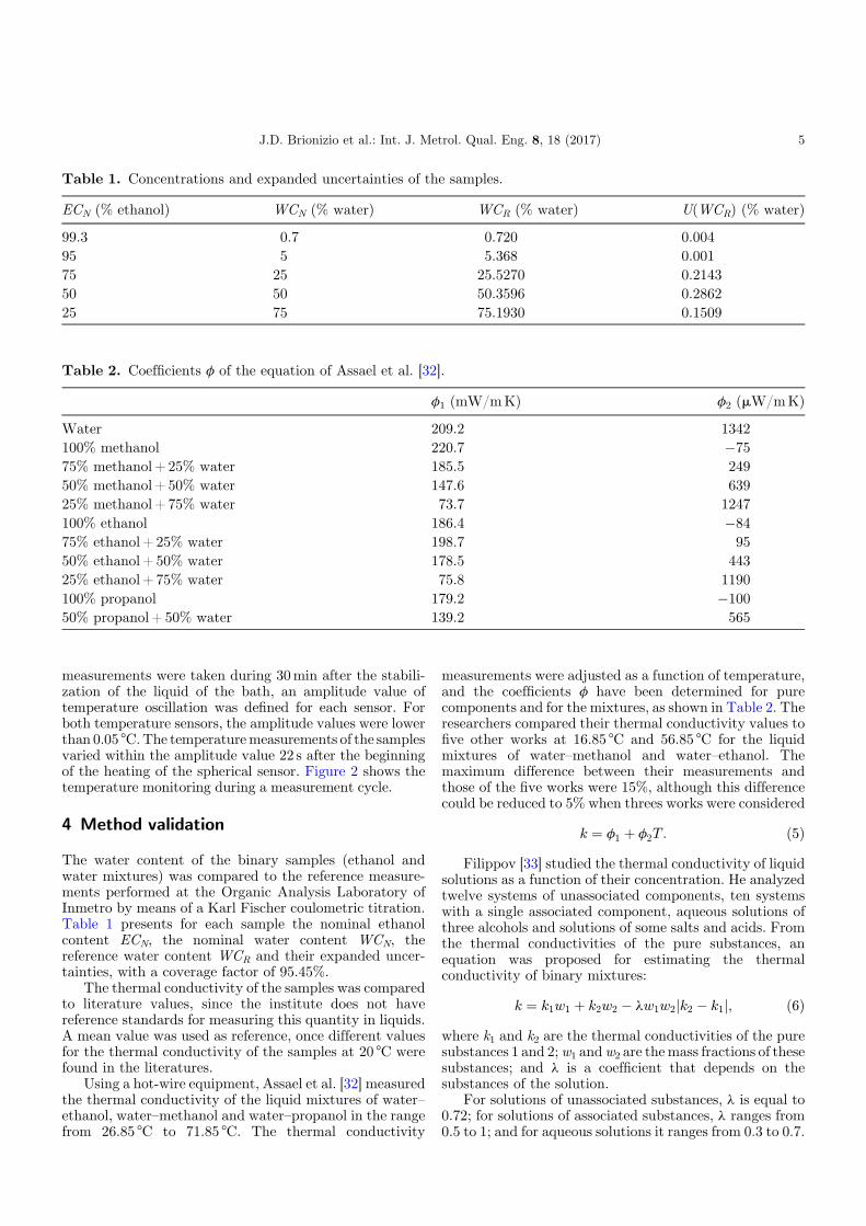
Table 1. Concentrations and expanded uncertainties of the samples.

ECN (% ethanol) WCN (% water) WCR (% water) U(WCR) (% water)

99.3 0.7 0.720 0.00495 5 5.368 0.00175 25 25.5270 0.214350 50 50.3596 0.286225 75 75.1930 0.1509

Table 2. Coefficients f of the equation of Assael et al. [32].

f1 (mW/mK) f2 (mW/mK)

Water 209.2 1342100% methanol 220.7 �7575% methanol+ 25% water 185.5 24950% methanol+ 50% water 147.6 63925% methanol+ 75% water 73.7 1247100% ethanol 186.4 �8475% ethanol+ 25% water 198.7 9550% ethanol+ 50% water 178.5 44325% ethanol+ 75% water 75.8 1190100% propanol 179.2 �10050% propanol+ 50% water 139.2 565

J.D. Brionizio et al.: Int. J. Metrol. Qual. Eng. 8, 18 (2017) 5

measurements were taken during 30min after the stabili-zation of the liquid of the bath, an amplitude value oftemperature oscillation was defined for each sensor. Forboth temperature sensors, the amplitude values were lowerthan 0.05 °C.The temperaturemeasurements of the samplesvaried within the amplitude value 22 s after the beginningof the heating of the spherical sensor. Figure 2 shows thetemperature monitoring during a measurement cycle.

4 Method validation

The water content of the binary samples (ethanol andwater mixtures) was compared to the reference measure-ments performed at the Organic Analysis Laboratory ofInmetro by means of a Karl Fischer coulometric titration.Table 1 presents for each sample the nominal ethanolcontent ECN, the nominal water content WCN, thereference water content WCR and their expanded uncer-tainties, with a coverage factor of 95.45%.

The thermal conductivity of the samples was comparedto literature values, since the institute does not havereference standards for measuring this quantity in liquids.A mean value was used as reference, once different valuesfor the thermal conductivity of the samples at 20 °C werefound in the literatures.

Using a hot-wire equipment, Assael et al. [32] measuredthe thermal conductivity of the liquid mixtures of water–ethanol, water–methanol and water–propanol in the rangefrom 26.85 °C to 71.85 °C. The thermal conductivity

measurements were adjusted as a function of temperature,and the coefficients f have been determined for purecomponents and for the mixtures, as shown in Table 2. Theresearchers compared their thermal conductivity values tofive other works at 16.85 °C and 56.85 °C for the liquidmixtures of water–methanol and water–ethanol. Themaximum difference between their measurements andthose of the five works were 15%, although this differencecould be reduced to 5% when threes works were considered

k ¼ f1 þ f2T : ð5ÞFilippov [33] studied the thermal conductivity of liquid

solutions as a function of their concentration. He analyzedtwelve systems of unassociated components, ten systemswith a single associated component, aqueous solutions ofthree alcohols and solutions of some salts and acids. Fromthe thermal conductivities of the pure substances, anequation was proposed for estimating the thermalconductivity of binary mixtures:

k ¼ k1w1 þ k2w2 � lw1w2jk2 � k1j; ð6Þwhere k1 and k2 are the thermal conductivities of the puresubstances 1 and 2;w1 andw2 are themass fractions of thesesubstances; and l is a coefficient that depends on thesubstances of the solution.

For solutions of unassociated substances, l is equal to0.72; for solutions of associated substances, l ranges from0.5 to 1; and for aqueous solutions it ranges from 0.3 to 0.7.

Table 3. Thermal conductivity values of the samples from literatures (inW/m °C) at 20 °C.

WCN (% water)

0 25 50 75 100

Assael et al. [32] � Eq. (5) 0.162 0.227 0.308 0.425 0.603Fang et al. [41] 0.164 0.229 0.315 0.445 0.598Filippov [33] � Eq. (6) – 0.230 0.322 0.445 –

Reid [34] � Eq. (7) – 0.234 0.321 0.439 –

Melinder [42] – – 0.317 0.438 0.598KDB [37] � Eqs. (11) and (12) 0.169 – – – 0.609IAPWS [38] – – – – 0.598Ramires et al. [35] � Eq. (8) – – – – 0.598Vargaftik [43] 0.168 – – – –

Miller and Yaws [36] � Eq. (9) 0.169 – – – –

Touloukian et al. [34] � Eq. (10) 0.168 – – – –

Mean 0.1666 0.2300 0.3169 0.4384 0.6006Standard deviation of the mean 0.0013 0.0015 0.0025 0.0037 0.0019

6 J.D. Brionizio et al.: Int. J. Metrol. Qual. Eng. 8, 18 (2017)

According to Khan [34], based on 120 data, the value of lfor Filippov’s equation for liquidmixtures of water–ethanolin the range from �70 °C to 60 °C is 0.571066.

Reid et al. have also proposed an equation for estima-ting the thermal conductivity of binary mixtures as afunction of the concentrations and thermal conductivitiesof the pure substances [34]:

k ¼ ðk1wl1 þ k2w

l2Þ1=l: ð7Þ

According to Khan [34], the value of l for the equationof Reid et al. for liquid mixtures of water–ethanol in therange from �70 °C to 60 °C is 0.051892.

From several experimental measurements performedby the hot-wire method, Ramires et al. [35] proposed anequation for estimating the thermal conductivity of waterin the range from 0.85 °C to 96.85 °C at atmosphericpressure:

k ¼ 0:6065

� �1:48445þ 4:12292T

298:15

� �� 1:63866

T

298:15

� �2" #

:

ð8Þ

Miller and Yaws proposed an equation for estimatingthe thermal conductivity of ethanol in the range from�114 °C to 190 °C [36]:

k ¼ 0:26293� 3:8468 � 10�4T þ 2:2106 � 10�7T 2: ð9Þ

Touloukian et al. proposed an equation for estimatingthe thermal conductivity of pure liquids, where for ethanolin the range from �123 °C to 127 °C the coefficients l1 and

l2 are 609.512 and �0.70924, respectively [34]:

k ¼ ðl1 þ l2T Þ � 0:0004187: ð10ÞThe Korea Thermophysical Properties Data Bank

(KDB), which provides information and estimatingmethods for the thermophysical properties of severalsubstances, presents the following equations for estimatingthe thermal conductivities of water (in the range from�0.15 °C to 349.85 °C) and ethanol (in the range from�113.15 °C to 189.85 °C), respectively [37]:

k ¼ �0:3838þ 0:005254T � 6:369 � 10�6T 2; ð11Þ

k ¼ �0:2629� 0:0003847T þ 2:211 � 10�7T 2: ð12ÞThe International Association for the Properties of

Water and Steam (IAPWS), a non-profit associationof national organizations concerned with the properties ofwater and steam, provides in its website an onlinecalculator, prepared by Moscow Power EngineeringInstitute and Russian National Committee of IAPWS,for estimating the thermal conductivity of water as afunction of temperature and density [38]. The calculatorwas based on the “Release on the IAPWSFormulation 2011for the Thermal Conductivity of Ordinary Water Sub-stance” [39]. The density of water was estimated by theequation presented by Tanaka et al. [40]. The output valueof thermal conductivity is presented in Table 3.

For estimating the thermal conductivity values of thebinary samples by means of the equations (6) and (7), thethermal conductivities of the pure substances werenecessary. In these cases, the thermal conductivities ofethanol and water were obtained, respectively, from KDB[37] and IAPWS [38]. Besides the thermal conductivity

J.D. Brionizio et al.: Int. J. Metrol. Qual. Eng. 8, 18 (2017) 7

values estimated by the aforementioned equations forwater, ethanol and their mixtures, Table 3 also presentsvalues which were interpolated or directly obtained intables available in literatures [41–43].

5 Preliminary results

For each sample, three measurement cycles were per-formed, and for each cycle a temperature step wasdetermined as:

DT ¼ Tf � T

i; ð13Þ

where, DT is the temperature step; Tiis the mean

temperature of the five readings before the heating of thesphere; and T

fis the last five readings during the heating of

sphere.As explained before, during the calibration of the

thermometers it was observed that the measurementsvaried within the range of 0.05 °C in a stabilized medium.This parameter was adopted as criterion to determine thesteady-state condition, which was reached 22 s after theheating of the sphere. The temperature step could then bedetermined in approximately 30 s. However, a slightlylonger measuring time was used.

Knowing the radius of the sphere, the heat transfer rate(electrical power) and the temperature step (measured asdetailed in Sect. 3), the thermal conductivities of thesamples could then be determined by means of equation(2). Nevertheless, the estimated results were highlyunsatisfactory, since they were very diverging from theliterature values shown in Table 3. The percentagedifferences from the estimated values to the literatureones increased from approximately 10–130% (sensor 01)and 30–160% (sensor 02) as the ethanol content increased.

Another option could be to use an effective radiusinstead of the geometrical radius of the sphere. An effectiveradius, which can be estimated by the calibration of thespherical sensor in certain substances (selected by the useraccording to his measurement needs), consists of a virtualradius that compensates the lack of knowledge of someparameters involved in the measurement process, so as toaccurately reproduce the thermal conductivities of thesubstances taken as reference. Using the thermal conduc-tivities of the samples as reference (Tab. 3), the heattransfer rate and the temperature steps, the effective radiifor each sensor could be estimated. Nevertheless, for bothsensors, the effective radii varied considerably from onesample to another. The effective radius of the sensorsincreased linearly as the ethanol content increased. Theestimated effective radii for sensors 01 and 02 wererespectively 1.28mm and 1.34mm for distilled water,and 2.67mm and 2.73mm for anhydrous ethanol. Dueto these considerable variations, the results were not usefulfor the measurement of the ethanol and water mixtures,because it would be necessary to use an effec-tive radius value according to the concentration of thesample to be measured, which is usually unknowninformation in practice. Except for the half and halfsample, the use of a mean effective radius is not convenient

either. The percentage differences from the estimatedthermal conductivities to the literature values increased asthe difference of the concentrations of the solutionsincreased, reaching approximately 35% in the pure sub-stances (distilled water and anhydrous ethanol).

The determination of the thermal conductivityvalues of the samples by the previous methods did notsucceed, because equation (2) should only be used in idealmodels, i.e., free from error sources. Nevertheless, the realprocess presents errors. So, a new model needed to bedeveloped.

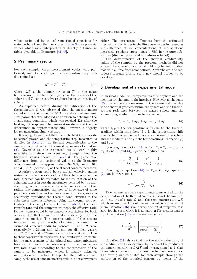
6 Development of an experimental model

In an ideal model, the temperatures of the sphere and themedium are the same in the interface. However, as shown in[25], the temperature measured in the sphere is shifted dueto the thermal gradient within the sphere and the thermalcontact resistance between the heated sphere and thesurrounding medium. It can be stated as:

Ts ¼ Tm þ dTG þ dTR ¼ Tm þ dT ; ð14Þwhere dTG is the temperature shift due to the thermalgradient within the sphere; dTR is the temperature shiftdue to the thermal contact resistance between the sphereand the medium; and dT is the temperature shift due to dTGand dTR.

Rearranging equation (14) as dT=Ts�Tm, and usingequations (2) and (4), dT can be deduced as:

dT ¼_Q

4prs

1

2ks� r2

2ksr2sþ 1

rsHc

� �: ð15Þ

Rearranging equation (14) as Tm=Ts� dT, equation(2) can be rewritten as:

k ¼_Q

4prsðTs � dT Þ : ð16Þ

Two parameters were experimentally measured for thedetermination of the thermal conductivities of the samples:the heat transfer rate _Q and the temperature step DT,which means that k should be expressed as a function ofthem. Equation (16) is valid when the initial temperature iszero; for the cases where it is not zero, DT is used instead ofTs. So, equation (16) can be rearranged as:

k ¼_Q

DT� 1

4prs 1� dTDT

24

35: ð17Þ

Equation (17) shows that the thermal conductivity ofthe medium can be determined by means of the product ofthe experimental ratio _Q=DT and a term, named as j, thattakes into consideration the possible temperature errors.The term j was calculated for each sample through thecalibration of the spherical sensors by means of the

Table 4. Experimental ratios _Q=DT and j for each sample obtained at 20 °C.

WCN (% water) kL Sensor 01 Sensor 02

W/m °C_Q=DT

j_Q=DT

j

W/°C m�1 W/°C m�1

0 0.1666 5.598� 10�3 29.8 5.715� 10�3 29.225 0.2300 6.433� 10�3 35.8 6.692� 10�3 34.450 0.3169 7.556� 10�3 41.9 7.704� 10�3 41.175 0.4384 8.859� 10�3 49.5 8.754� 10�3 50.1

100 0.6006 9.680� 10�3 62.0 10.102� 10�3 59.4

Table 5. Thermal conductivities of the samples by the developed model (inW/m °C) at 20 °C.

Sensor WCN (% water)

100 75 50 25 0

k D% k D% k D% k D% k D%

01 0.598 �0.4 0.441 0.6 0.318 0.3 0.230 0.0 0.165 �1.00.600 �0.1 0.437 �0.3 0.317 0.0 0.231 0.4 0.166 �0.40.603 0.4 0.437 �0.3 0.317 0.0 0.230 0.0 0.170 2.0

02 0.601 0.1 0.434 �1.0 0.314 �0.9 0.225 �2.2 0.166 �0.40.603 0.4 0.440 0.4 0.319 0.7 0.230 0.0 0.167 0.20.597 �0.6 0.439 0.1 0.321 1.3 0.232 0.9 0.167 0.2

8 J.D. Brionizio et al.: Int. J. Metrol. Qual. Eng. 8, 18 (2017)

following equation:

j ¼ kL_Q=DT

; ð18Þ

where kL is the mean thermal conductivity of the sampleobtained from literature.

Table 4 presents for each sample the experimental ratio_Q=DT , which is a mean value of the three measurementcycles, kL and the terms j.

An equation relating the experimental ratios _Q=DT andthe terms j could be adjusted for each sensor. This equationis the calibration curve of the instrument. It means that,knowing _Q and measuring DT, the equation compensatesthe errors of the sensor and gives the thermal conductivityvalue for water, ethanol and any unknownmixture betweenthese substances. Nevertheless, as the thermal conductivi-ties of the binary samples do not vary linearly with thewater content, a polynomial function is the best option.Thus, a third degree equation (with coefficient ofdetermination equals 1) was then chosen for each sensor:

Sensor 01 : � 1:877 � 10�7j3 þ 2:341 � 10�5j2

� 7:873 � 10�4j

þ 1:324 � 10�2 �_Q

DT

� �¼ 0; ð19Þ

Sensor 02 : 1:118 � 10�7j3 � 1:561 � 10�5j2

þ 8:441 � 10�4j

� 8:403 � 10�3 �_Q

DT

� �¼ 0: ð20Þ

Table 5 presents the thermal conductivities of thesamples, determined by means of the equations (19) and(20), for the three measurement cycles, and the percentagedifferences D% from the estimated values to the literatureones.

Unlike the previous cases, the determination of thethermal conductivity values of the samples by thedeveloped model was successful. The thermal conductivi-ties estimated for the measured samples clearly presentsmall divergences from the literature values, which showthat the equations set for the sensors by means ofcalibration are fairly good.

The developed experimental model worked because theerrors of the real measurement process were compensatedby the calibration. As shown by equation (15), some errorsof the measurement process come from the lack of someinformation, such as the thermal conductivity of thesphere, the right positioning of the temperature sensorwithin the sphere and the thermal resistance between thesphere and the medium. In addition, other phenomenamayalso cause errors in the process, such as the influence of the

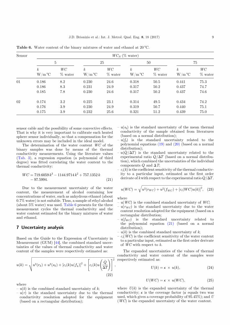
Table 6. Water content of the binary mixtures of water and ethanol at 20 °C.

Sensor WCN (% water)

5 25 50 75

k WC k WC k WC k WCW/m °C % water W/m °C % water W/m °C % water W/m °C % water

01 0.186 8.2 0.230 24.6 0.318 50.5 0.441 75.30.186 8.3 0.231 24.9 0.317 50.2 0.437 74.70.185 7.8 0.230 24.6 0.317 50.2 0.437 74.6

02 0.174 3.2 0.225 23.1 0.314 49.5 0.434 74.20.176 3.9 0.230 24.9 0.319 50.7 0.440 75.10.175 3.9 0.232 25.6 0.321 51.2 0.439 75.0

J.D. Brionizio et al.: Int. J. Metrol. Qual. Eng. 8, 18 (2017) 9

sensor cable and the possibility of some convective effects.That is why it is very important to calibrate each heatedsphere sensor individually, so that a compensation for theunknown errors may be included in the ideal model.

The determination of the water content WC of thebinary samples was done by means of the thermalconductivity measurements. Using the literature values(Tab. 3), a regression equation (a polynomial of thirddegree) was fitted correlating the water content to thethermal conductivity:

WC ¼ 719:6059 k3 � 1144:9714 k2 þ 757:1352 k� 97:5994: ð21Þ

Due to the measurement uncertainty of the watercontent, the measurement of alcohol containing lowconcentrations of water, such as anhydrous ethanol (about0.7% water) is not suitable. Thus, a sample of ethyl alcohol(about 5% water) was used. Table 6 presents for the threemeasurement cycles the thermal conductivity and thewater content estimated for the binary mixtures of waterand ethanol.

7 Uncertainty analysis

;

Based on the Guide to the Expression of Uncertainty inMeasurement (GUM) [44], the combined standard uncer-tainties of the values of thermal conductivity and watercontent of the samples were respectively estimated as:

uðkÞ ¼

ffiffiffiffiffiffiffiffiffiffiffiffiffiffiffiffiffiffiffiffiffiffiffiffiffiffiffiffiffiffiffiffiffiffiffiffiffiffiffiffiffiffiffiffiffiffiffiffiffiffiffiffiffiffiffiffiffiffiffiffiffiffiffiffiffiffiffiffiffiffiffiffiffiffiffiffiffiffiffiffiffiffiffiffiffiffiffiffiffiffiffiffiffiffiffiffiffiffiffiffiffiffiu2ðrkÞ þ u2ðskÞ þ ½ciðkÞuðfkÞ�2 þ ciðkÞu

_Q

DT

!" #2vuutð22Þ

where

– u(k) is the combined standard uncertainty of k; – u(r) is the standard uncertainty due to the thermalconductivity resolution adopted for the equipment(based on a rectangular distribution);

–

u(sk) is the standard uncertainty of the mean thermalconductivity of the sample obtained from literatures(based on a normal distribution);

–

u(fk) is the standard uncertainty related to thepolynomial equations (19) and (20) (based on a normaldistribution);

–

uð _Q=DT Þ is the standard uncertainty related to theexperimental ratio _Q=DT (based on a normal distribu-tion), which combined the uncertainties of the individualcomponents _Q and DT;

–

ci(k) is the coefficient sensitivity of the thermal conductiv-ity to a particular input, estimated as the first orderderivate of kwith respect to the experimental ratio _Q=DT .

uðWCÞ ¼ffiffiffiffiffiffiffiffiffiffiffiffiffiffiffiffiffiffiffiffiffiffiffiffiffiffiffiffiffiffiffiffiffiffiffiffiffiffiffiffiffiffiffiffiffiffiffiffiffiffiffiffiffiffiffiffiffiffiffiffiffiffiffiffiffiffiffiffiffiffiffiffiffiffiffiu2ðrWCÞ þ u2ðfWCÞ þ ½ciðWCÞuðkÞ�2

q; ð23Þ

where

– u(WC) is the combined standard uncertainty of WC; – u(rWC) is the standard uncertainty due to the watercontent resolution adopted for the equipment (based on arectangular distribution;

–

u(fWC) is the standard uncertainty related tothe polynomial equation (21) (based on a normaldistribution);

–

u(k) is the combined standard uncertainty of k; – ci(WC) is the coefficient sensitivity of the water contentto a particular input, estimated as the first order derivateof WC with respect to k.

The expanded uncertainties of the values of thermalconductivity and water content of the samples wererespectively estimated as:

UðkÞ ¼ k � uðkÞ; ð24Þ

UðWCÞ ¼ k � uðWCÞ; ð25Þwhere U(k) is the expanded uncertainty of the thermalconductivity; k is the coverage factor (k equals two wasused, which gives a coverage probability of 95.45%); and U(WC) is the expanded uncertainty of the water content.

Table 7. Uncertainties for the thermal conductivities of the samples.

Sensor WCN (% water) u(rk) u(sk) ci(k)u(fk) ci(k)u( _Q=DT ) u(k) U(k) U(k)W/m °C W/m °C W/m °C W/m °C W/m °C W/m °C %

01 0 0.000289 0.0013 0.0007 0.0032 0.0035 0.007 4.225 0.000289 0.0015 0.0006 0.0053 0.0056 0.011 4.850 0.000289 0.0025 0.0007 0.0074 0.0079 0.016 5.075 0.000289 0.0037 0.0009 0.0087 0.0095 0.019 4.3

100 0.000289 0.0019 0.0011 0.0138 0.0139 0.028 4.7

02 0 0.000289 0.0013 0.0014 0.0047 0.0050 0.010 6.025 0.000289 0.0015 0.0019 0.0055 0.0060 0.012 5.250 0.000289 0.0025 0.0025 0.0088 0.0095 0.019 6.075 0.000289 0.0037 0.0030 0.0132 0.0140 0.028 6.4

100 0.000289 0.0019 0.0029 0.0178 0.0181 0.036 6.0

Table 8. Uncertainties for the water content of the binary mixtures.

Sensor WCN (% water) u(rWC) u(fWC) ci(WC)u(k) u(WC) U(WC)% water % water % water % water % water

01 5 0.029 0.390 1.583 1.63 3.325 0.029 0.390 1.891 1.93 3.950 0.029 0.390 1.980 2.02 4.175 0.029 0.390 1.586 1.63 3.3

02 5 0.029 0.390 2.324 2.36 4.825 0.029 0.390 2.029 2.07 4.250 0.029 0.390 2.315 2.35 4.775 0.029 0.390 2.493 2.52 5.1

10 J.D. Brionizio et al.: Int. J. Metrol. Qual. Eng. 8, 18 (2017)

It is worth pointing out that the reproducibility of DT isdue to the reproducibility of the temperature measure-ments, which was estimated during the calibration of thethermometer (by means of the repetition of the calibrationpoint 20 °C) and included in its uncertainty. Therepeatability of DT was estimated during the temperaturemeasurements of the samples as the standard deviation ofthe mean values (before and during the heating of thesphere). In the case of _Q, the reproducibility consists onhow the equipment reproduces the heat generation. It wasestimated during the characterization of the equipment (bymeans of the repetition of three calibration points) andincluded in its uncertainty. The repeatability of _Q was alsoestimated during the characterization of the equipment bymeans of the standard deviation of the mean values ofvoltage and current and included in its uncertainty.

Table 7 presents the standard uncertainties, thecombined standard uncertainty, the expanded uncertaintyand the percentage expanded uncertainty of the thermalconductivity determined for each sample.

Table 8 presents the standard uncertainties, thecombined standard uncertainty and the expanded uncer-tainty of the water content determined for each sample.

8 Comparing the resultsThe thermal conductivity values reported in someliteratures were not provided with their uncertaintystatements or error estimations. So, the agreement ofthe measured values with the literature ones was checkedby means of the percentage expanded uncertainties of thethermal conductivities determined for the samples. Thepercentage differences between all the values of thermalconductivity given in the literatures (by means of tables orby the equations from (6) to (12)) and the mean thermalconductivity measured for each sample (calculated bymeans of the values of the three measurement cycles) weresmaller than its percentage expanded uncertainty, whichconfirm the agreement of the measured values with theliterature ones. Figures 3 (sensor 01) and 4 (sensor 02) showthe difference between each literature value and the meanthermal conductivity, and the uncertainty of the thermalconductivity measurement of each sample.

It can be clearly seen by means of Figures 3 and 4 thatthere is a good agreement between the measured thermalconductivities and the literature ones for all the samples,which validates the developed method for measuring thethermal conductivity of water, ethanol and their mixtures.

-0.04

-0.03

-0.02

-0.01

0.00

0.01

0.02

0.03

0.04

0 25 50 75 100

erutare tilk

-.

m/W/

de rusaem

kC

Samples at 20 ºC/ %water

Assael et al. Fang et al. Filippov ReidMelinder KDB IAPWS Ramires et al.Vargaftik Miller e Yaws Touloukian et al.

Fig. 4. Differences between literature values and the mean thermal conductivity for sensor 02.

Table 9. Comparison of the measurements of WC of the binary samples (in % water).

WCN WCR U(WCR) Sensor 01 Sensor 02

WC U(WC) En WC U(WC) En

5 5.368 0.001 8.2 3.3 0.8 3.2 4.7 0.58.3 3.3 0.9 3.9 4.7 0.37.8 3.3 0.7 3.9 4.7 0.3

25 25.5270 0.2143 24.6 3.9 0.2 23.1 4.1 0.624.9 3.9 0.2 24.9 4.1 0.224.6 3.9 0.2 25.6 4.1 0.0

50 50.3596 0.2862 50.5 4.0 0.0 49.5 4.7 0.250.2 4.0 0.0 50.7 4.7 0.150.2 4.0 0.0 51.2 4.7 0.2

75 75.1930 0.1509 75.3 3.3 0.0 74.2 5.0 0.274.7 3.3 0.1 75.1 5.0 0.074.6 3.3 0.2 75.0 5.0 0.0

-0.03

-0.02

-0.01

0.00

0.01

0.02

0.03

0 25 50 75 100

erutaretilk

-.

m/W/

deruaem

kC

Samples at 20 ºC / %water

Assael et al. Fang et al. Filippov ReidMelinder KDB IAPWS Ramires et al.Vargaftik Miller e Yaws Touloukian et al.

Fig. 3. Differences between literature values and the mean thermal conductivity for sensor 01.

J.D. Brionizio et al.: Int. J. Metrol. Qual. Eng. 8, 18 (2017) 11

12 J.D. Brionizio et al.: Int. J. Metrol. Qual. Eng. 8, 18 (2017)

In order to validate the water content determined forthe binary samples, these were compared to the referencemeasurements performed at Inmetro and presented inTable 1. The compatibility of the measurements waschecked by means of the normalized error (En), which iscalculated according to the following equation [45]:

En ¼ WC �WCRffiffiffiffiffiffiffiffiffiffiffiffiffiffiffiffiffiffiffiffiffiffiffiffiffiffiffiffiffiffiffiffiffiffiffiffiffiffiffiffiffiffiffiffiffiUðWCÞ2 þ UðWCRÞ2

q : ð26Þ

Table 9 shows the reference measurements of the watercontent of the binary samples, the values determined bythe developed method in this study and the normalizederrors.

A comparison between two measurements is satisfac-tory when |En|� 1. Consequently, the water contentmeasurements of this work and those performed by thereference laboratory are clearly compatible, since all the Envalues were lower than one, validating the developedmethod for measuring the water content of binary samplesof water and ethanol.

9 Conclusions

The method of the spherical heat source, in principle, is anabsolute measuring method of thermal conductivity,which means that the sensor can provide an outputwithout being calibrated against a standard or a referencematerial. However, some parameters of the model need tobe carefully taken into consideration. Thus, to compensatefor the lack of some theoretical evaluations and thedifficulty for obtaining accurately some practical informa-tion, the heated sphere sensors needed to be calibrated bymeans of mediums with known thermal properties. As thedevices have different constructive characteristics fromeach other, the calibration must be done individually.

The use of spherical heat sources in the industrialsectors for measuring the thermal conductivity presentsconsiderable advantages, such as wide measuring range,relatively fast measurements, measurement uncertaintycompatible with other techniques and the possibility ofusing the sensor in situ. The method has also a greatpotential to be employed in research institutes andlaboratories that provide calibration and testing services.

The applicability of the method of the spherical heatsource for measuring the thermal conductivity of water,ethanol and their mixtures proved to be quite satisfactory,since the measurements of this study showed excellentagreement with the values proposed by several researchers.This agreement occurred with values obtained by othermeasurement methods, such as the traditional hot-wiretechnique, as with those obtained bymeans of equations forestimating the thermal conductivity. The applicability ofthe method for determining the water content of the binarysamples was also quite satisfactory, since the results of theproposed method showed good agreement with thoseperformed by the reference equipment from the nationalinstitute (Inmetro).

10 Implications and influences

The paper presents the metrological aspects and thecalibration procedure of a spherical heat source to measurethermal conductivity and water content of some liquidsamples. This will strongly contribute and stimulate futureworks on the investigation of the applicability of thespherical heat source method and its metrological aspectsfor measuring thermal conductivity and water content ofother liquids and other mediums.

References

1. M.J. Assael, K.D. Antoniadis, W.A. Wakeham, Int. J.Thermophys. 31, 1051 (2010)

2. ASTM D-2717-15, Standard Test for Thermal Conductivityof Liquids (American Society for Testing and Materials,Philadelphia, PA, 2009)

3. U. Hammerschmidt, W. Sabuga, Int. J. Thermophys. 21,1255 (2000)

4. F.A. Gibbs, Proc. Soc. Exp. Biol. Med. 31, 141 (1933)5. J. Grayson, J. Physiol. 114 (Suppl.), 29 (1951)6. W. Chester, J. Grayson, Nature 4273, 521 (1951)7. J. Grayson, J. Physiol. 118, 54 (1952)8. H.S. Carslaw, in Introduction to the Mathematical Theory

of the Conduction of Heat in Solids (Macmillan, London,1921), 2nd ed.

9. J.C. Chato, Therm. Prob. Biotechnol. Trans. ASME 16(1968)

10. T.A. Balasubramaniam, H.F. Bowman, J. Heat Trans.Trans. ASME 296 (1974)

11. R.K. Jain, J. Biomech. Eng. Trans. ASME 101, 82 (1979)12. M.M. Chen, K.R. Holmes, V. Rupinskas, J. Biomech. Eng.

Trans. ASME 103, 253 (1981)13. J.W. Valvano, The use of thermal diffusivity to quantify

tissue perfusion, Ph.D. thesis, Harvard University, 198114. G. Hamilton, Investigation of the thermal properties of

human and animal tissues, Ph.D. thesis, University ofGlasgow, 1998

15. H. Zhang, S. Cheng, L. He, A. Zhang, Y. Zheng, D. Gao, CellPreserv. Technol. 1, 141 (2002)

16. K.A. Woodbury, Experimental and analytical investigationof liquid moisture distribution in roof insulating systems,Ph.D. thesis, Virginia Polytechnic Institute and StateUniversity, 1984

17. M. Fujii, H. Takamatsu, T. Fujii, in Proceedings of the 1stAsian Thermophysical Properties Conference, Beijing, 1986,edited by W. Buxuan et al. (China Academic Publishers,Beijing, 1986), pp. 462–467

18. B.P. Dougherty, An automated probe for thermal conduc-tivity measurements, M.Sc. thesis, Virginia PolytechnicInstitute and State University, 1987, cited in [22]

19. R.R. Kravets, Determination of thermal conductivity of foodmaterials using a bead thermistor, Ph.D. thesis, VirginiaPolytechnic Institute and State University, 1988, cited in [22]

20. U.B. Holeschovsky, G.T. Martin, J.W. Tester, Int. J. HeatMass Transf. 39, 1135 (1996)

21. S. Radhakrishnan, Measurement of thermal properties ofseafood, M.Sc. thesis, Virginia Polytechnic Institute andState University, 1997

J.D. Brionizio et al.: Int. J. Metrol. Qual. Eng. 8, 18 (2017) 13

22. M.F. Gelder, A thermistor based method for the measure-ment of thermal conductivity and thermal diffusivity ofmoist food materials at high temperatures, Ph.D. thesis,Virginia Polytechnic Institute and State University, 1998

23. H. Zhang, L. He, S. Cheng, Z. Zhai, D. Gao, Meas. Sci.Technol. 14, 1396 (2003)

24. L. Kubicar, L. Bagel, V. Vretenar, V. Stofanik, inProceedingsof theMeeting of the Thermophysical Society –Thermophysics2005, Kocovce, 2005, edited by P. Matiasovsky, O.Koronthalyova (ICA SAS, Bratislava, 2005), pp. 38–42

25. L. Kubicar, V. Vretenar, V. Stofanik, V. Bohac, Int. J.Thermophys. (2008), doi:10.1007/s10765-008-0544-4

26. L. Kubicar, U. Hammerschmidt, D. Fridrikova, P. Dieska, V.Vretenar, inProceedingsofThermophysics2010,Valtice, 2010(Brno University of Technology, Brno, 2010), pp. 166–171

27. J. Goldemberg, L.A.H. Nogueira, http://bioenergyconnection.org/article/sweetening-biofuel-sector-history-sugarcane-ethanol-brazil, accessed on May 2016

28. H.S. Carslaw, J.C. Jaeger, in Conduction of Heat in Solids(Oxford University Press, London, 1959), 2nd ed.

29. H.F. Bowman, T.A. Balasubramaniam, Cryobiology 13, 572(1976)

30. J.W. Valvano, J.R. Cochran, K.R. Diller, Int. J. Thermo-phys. 6, 301 (1985)

31. R.J. Schmidt, S.W. Milverton, Proc. Roy. Soc. Lond. A:Mater. 152, 586 (1935)

32. M.J. Assael, E. Charitidou, W.A. Wakeham, Int. J.Thermophys. 10, 793 (1989)

33. L.P. Filippov, Int. J. Heat Mass Transf. 11, 331 (1968)34. M.H. Khan, Modeling, simulation and optimization of

ground source heat pump systems, M.Sc. thesis, OklahomaState University, 2004

35. M.L.V. Ramires, C.A.N. de Castro, Y. Nagasaka, A.Nagashima, M.J. Assael, W.A. Wakeham, J. Phys. Chem.Ref. Data 24, 1377 (1995)

36. S. Henke, P. Kadlec, Z. Bubník, J. Food Eng. 99, 497 (2010)37. Korea Thermophysical Properties Data Bank, KDB: Pure

Components Properties (2012), available on http://www.cheric.org, accessed on 2012

38. IAPWS, Online Calculation for General and Scientific Use(2012), available on http://www.iapws.org/relguide/ThCond.html, accessed on 2012

39. IAPWS, Release on the IAPWS Formulation 2011 for theThermal Conductivity of Ordinary Water Substance (2012),available on http://www.iapws.org/release.html, accessedon 2012

40. M. Tanaka, G. Girard, R. Davis, A. Peuto, N. Bignell,Metrologia 38, 301 (2001)

41. L.Q. Fang, L.R. Sen, N.D. Yan, H.Y. Chun, J. Chem. Eng.Data 42, 971 (1997)

42. A. Melinder, Thermophysical properties of aqueous solutionsused as secondary working fluids, Ph.D. thesis, RoyalInstitute of Technology, 2007

43. B.E. Polin, J.M. Prausnitz, J.P. O’Connell, inThe Propertiesof Gases and Liquids (McGraw-Hill, NewYork, 2001), 5th ed.

44. INMETRO, Avaliação de Dados de Medição: Guia para aExpressãoda Incerteza deMedição�GUM2008 (INMETRO,Rio de Janeiro, 2012), 1st ed.

45. Conformity Assessment � General Requirements for Profi-ciency Testing, ISO/IEC 17043 (International Organizationfor Standardization and International ElectrotechnicalCommission, 2010)

Cite this article as: J�ulio Dutra Brionizio, Alcir de Faro Orlando, Georges Bonnier, Characterization of a spherical heat source formeasuring thermal conductivity and water content of ethanol and water mixtures, Int. J. Metrol. Qual. Eng. 8, 18 (2017)