Characterization and Radiative Impact of a Springtime Arctic Mixed-Phase Cloudy Boundary Layer observed during SHEBA

Paquita Zuidema

University of Colorado/NOAA Environmental Technology Laboratory, Boulder, CO

SHEBA Surface Heat Budget of the Arctic

Early May~ 76N, 165 W

WHY ?

• GCMs indicate Arctic highly responsive to increasing greenhouse gases (e.g. IPCC)

• Clouds strongly influence the arctic surface andatmosphere, primarily through radiative interactions

• Factors controlling arctic cloudiness not well known

Observational evidence may support predictions: (Serreze et al. 2000)

Arctic Sea Ice Extent in 2002 strongly diminished relative to 1987-2001 mean

Annual warming dominated by winter and spring spring warming ~ 0.5 C/decade in SHEBA region

Spring 1966-1995 Temperature Trends (Serreze et al., 2000; Jones 1994)

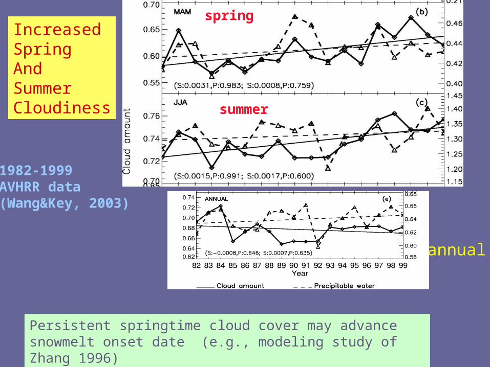
annual

IncreasedSpringAndSummerCloudiness

1982-1999AVHRR data(Wang&Key, 2003)

Persistent springtime cloud cover may advance snowmelt onset date (e.g., modeling study of Zhang 1996)

spring

summer

Project Goal

• characterize a multi-day arctic cloud sequence as best possible• elucidate the underlying cloud physical processes• assess the cloud’s radiative impact.

The Case: May 1- May 10, 1998.Surface-based, mixed-layer, mixed-phase cloud

Overlaps with the first two FIRE.ACE* flights*Arctic Clouds Experiment

The challenge: both ice and liquid phases are present

Surface-based Instrumentation: May 1-8 time series

35 GHz cloud radarice cloud properties

depolarization lidar-determined liquid cloud base

Microwave radiometer-derived liquid water paths

4X daily soundings. Near-surface T ~ -20 C, inversion T ~-10 C

-5-45 -20

1 2 3 4 5 6 7 8day

z

-30C

41 8

2

4

6

8

km

100g/m^2

day

-10C

lidar cloud base

1) Radar-based estimates of ice cloud properties applied to estimate ice component within mixed-phase conditions, requires validation

2) Adiabatic characterization of liquid phase, requires additional info.

ISSUES:

SURFACE INSTRUMENTATION PURPOSE HOW

cloud radar (35 GHz f, 8.6 mm ) Ice phase properties Matrosov et al. (2002,2003)

depolarization lidar liquid water cloud base Intrieri et al. (2002)(0.5235 m )

4X daily soundings T, RH

microwave radiometer (23.8 & 31.8 GHz f) liquid water path Yong Han physical retrieval

ICE

LIQUID (adiabatic characterization)

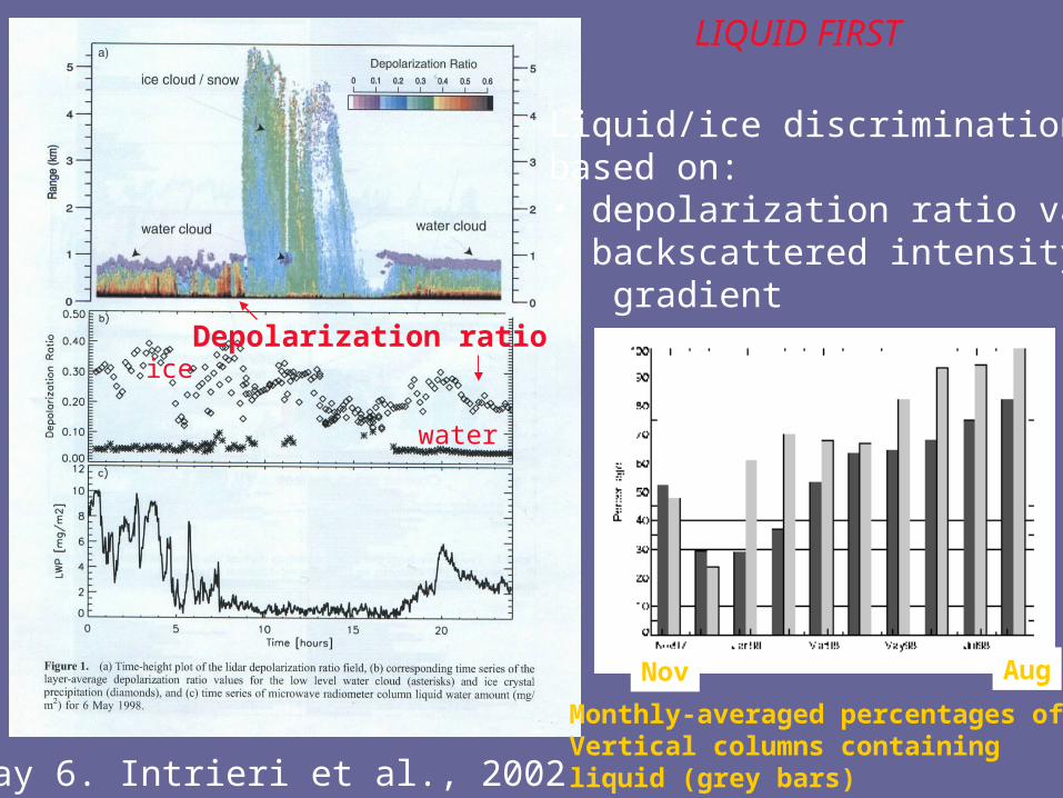
May 6. Intrieri et al., 2002

Depolarization ratioice

water

Liquid/ice discriminationbased on:• depolarization ratio value• backscattered intensity gradient

Monthly-averaged percentages ofVertical columns containing liquid (grey bars)

Nov Aug

LIQUID FIRST

wavelength

Frequency (GHZ)

Clough et al., ‘89

Microwave-radiometer-derivedLiquid water paths:

• microwave radiometer responds to integrated water vapor and liquid water

• physical retrieval also utilizes:- cloud temperature- soundings

• decreased uncertainty (good for Arctic conditions)

• Yong Han, unpublished data

adiabatic calculation constrained by……

May 4 & 7 NCAR C130

Research Flights

• FSSP-100 2-47 liquid, ice size distribution

• 1D OAP-260X (May 4) 40-640 ice size distribution

• 2D OAP (May 7) 25-800 ice shape, size

• Cloud Particle Imager 5-2000 particle phase, shape, size

• King hot-wire probe liquid water content

range (micron) parameterinstrument

establishes liquid droplet concentration and distribution width

Aircraft path

Lidar cloud base

Temperature inversion

Cloud radar reflectivity

time

Hei

gh

t (k

m)

1

2

dBZ0-50-50

May 4

24:0022:00 23:00UTC

Liquid Characterization

Liquid Water Content: Adiabatic Ascent Calculation

• lidar-determined liquid cloud base parcel

• interpolated sounding temperature structure

• constrained w/ microwave radiometer-derived liquid water path

King LWC

adiabatic LWC

CB

excellent correspondencebetween adiabatic calc. andKing probe LWC

May 4

Z(km)

Liquid water content g/m^3

0 0.5

0.6

1.0

Derivation of liquid volume extinction coefficient and effective particle radius re

• Lognormal droplet size distribution

<rk> = <rok>exp(k22/2) (Frisch et

al., ’95,’98,’02)

• mean aircraft cloud droplet conc.

N=222 (14)

• mean aircraft lognormal of geometric standard deviation of droplet size distribution

0.242 (0.04)

May 4

re

adiabatic

aircraft

May 7: thin cloud, low LWP

Lidar depolarization ratio

High aerosols ! Max of 1645/L(Rogers et al., 2001)

Backscattered intensity

May 1 – 10 liquid re, time series

re

day2

0 30

0

3 4 5 86 71 day

0

30

Mean liquid cloud optical depth ~ 10, mean r_e ~4.5

re

May 1-3 Mean Sea Level Pressure

May 4-9 Mean Sea Level Pressure

Weak low N/NW of shipfollowed by weak/broad high moving from SW to NE

Data courtesy of NOAA Climate Diagnostics Center

Boundary-layer depth synchronizes w/ large-scalesubsidence

ICE microphysics retrieval• radar only (Matrosov et al. 2002; 2003)• particle size retrieved from Doppler velocity• particle mass retrieved from reflectivity & particle size

MAY 5

• Radar retrieval developed for ice clouds, not ice+liquid clouds

• Radar not sensitive to the smaller particles

• Another degree of freedom: Particle shape

• for bulk aircraft measurements, complete size distributions difficult to form

Comparison to aircraft data uncertainIWC comparison most reliable (not D or

ISSUES:

May 4 Cloud Particle Imager data

…pristine ice particles from upper cloud

...super-cooled drizzle

May 4 complete size distribution: FSSP (*), CPI (line),260X (triangles)

Robust conclusions:• Radar reflectivity

insensitive to liquid

when ice is present

• Radar retrievals agree with aircraft-derived values given large uncertainties (~4x ?)

• Ice cloud optical depth almost insignificant

dBZ

liquid

radar

Ice aircraft

IWCDeff

What is the radiative impact of the ice ?

• Direct impact negligible: mean ice cloud optical depth ~0.2

BUT:• 1) upper ice cloud sedimentation

associated with near-complete or complete LWP dissipation* (May 4 & 6)

• 2) local IWC variability associated with smaller LWP changes, time scale ~ few hours

* At T=-20C, air saturated wrt water is ~ 20% supersaturated wrt ice

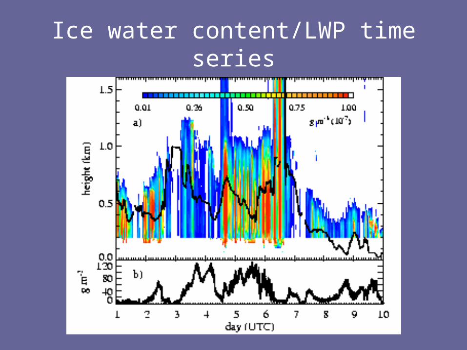
Ice water content/LWP time series

Mechanism for local ice production:

• Liquid droplets of diameter > ~ 20 micron freeze preferentially, grow, fall out

• New ice particles not produced again until collision-coalescence builds up population of larger drops

• Only small population of large drops required• Hobbs and Rangno, 1985; Rangno and Hobbs,

2001; Korolev et al. 2003; Morrison et al. 2004• Little previous documentation within cloud radar

data

Local ice production more evident when boundary layer is deeper and LWPs are higher

May 3 counter-example – variable aerosol entrainment ?

Quick replenishment of liquid: longer-time-scale variability in cloud optical depth related to boundary layer depth changes

Project Goal

• characterize a multi-day arctic cloud sequence as best possible• elucidate the underlying cloud physical processes• assess the cloud’s radiative impact.

The Case: May 1- May 10, 1998.Surface-based, mixed-layer, mixed-phase cloud

Overlaps with the first two FIRE.ACE* flights*Arctic Clouds Experiment

Radiative flux closure and cloud forcing

Implement derived cloud properties within radiative transfer model

Streamer (Key & Schweiger; Key 2001). Medium-bandcode, utilizes DISORT (Stamnes et al. 2000)

Strength: comprehensive, adapted for Arctic climate problems

• Both phases represented within a single volume• Shortwave ice cloud optical properties parameterized for 7 particle habits • Arctic aerosol profile available• surface albedo spectral variation adequately represented

Weakness: 4 gases only, outdated gaseous line information

• SHEBA spectral surface albedo data (Perovich et al.) time-mean broadband albedo = 0.86 (matches surface-flux albedo)

• Arctic haze aerosol profiles constrained with sunphotometer measurements (R. Stone, unpub. data) Aerosol optical depth = 0.135 @ 0.6 micron

• Ozone column amount = 393 DU (TOMS; J. Pinto pers. comm.)

Clear-sky comparison (May 7 & April 25)

Shortwave and infrared calculated and measured Downwelling surface fluxes agree to within 1 W/m^2

Most common ice particle habit: aggregate

(below liquid cloud base)

number area mass

spheresaggregates, small&big

Comparison of modeled to observed surface downwelling radiative fluxes, May 1 -8

• modeled LW > observed LW by 1 W m-2 ; RMS dev. = 13 W m-2 or 13% of observed fluxes

• modeled SW > observed SW by 3 W m-2 ; RMS dev. = 17 W m-2 or 12% of observed fluxes

• Bias slightly larger for low LWP cases

• Small bias encourages confidence in data (better agreement cannot be achieved w/out exceeding estimated uncertaintities)

modeled W m-2

ob

serv

ed

longwave shortwave

How do clouds impact the surface ?

noon = 60o

Clouds decrease surface SW by 55 W m-2 ,increase LW by 49 W m-2

Surface albedo=0.86; most SW reflected backClouds warm the surface, relative to clear skies with same T& T & RH, by time-mean 41 W m-2* (little impact at TOA)

• Can warm 1m of ice by 1.8 K/day, or melt 1 cm of 0C ice per day, barring any other mechanisms !

Shortwave

For cloud optical depth<3, net cloud forcing dominated by longwave=> Sensitive to optical depth changes

Longwave

Net

For cloud optical depth > 6, net cloud forcing dominated by shortwave=> Sensitive to solar zenith angle,surface reflectance changes

Cloud optical depth

~30% of cloud optical depths < 3~60% > 6

How sensitive is the surface to cloudiness changes ?

• Satellite-based study concludes surface cloud forcing most sensitive to changes in cloud amount, surface reflectance, cloud optical depth, cloud top pressure (Pavolonis and Key, 2003)

LWP (g m-2)+5+20-5-20

CF (W m-2)+2+3-3.5-10

surface

+0.05-0.05

CF (W m-2)

+4.5-3.8

Little radiative impact from additional waterSurface reflectance changes may be more radiatively significant

Why is this cloud so long-lived ????

• Measured ice nuclei concentrations are high (mean = 18/L, withMaxima of 73/L on May 4 and 1654/L (!) on May 7 (Rogers et al. 2001)

• This contradicts modeling studies that find quick depletion w/ IN conc of 4/L (e.g. Harrington et al. 1999)

Cloud-top radiative cooling rates can exceed 65 K/day

Strong enough cooling to maintain cloud for any IN value (Pinto 1998) Promotes turbulent mixing down to surface, facilitating surface fluxes

One part of the explanation:

How did this cloud finally dissipate ????

Strong variability in subsidence rates part of answer

Most interesting results:• Radiative flux impact of this mixed-phase cloud is close tothat of a pure liquid cloud

• Two mechanisms by which ice regulates the overall cloud optical depth:1) Sedimentation from upper ice clouds2) A local ice production mechanism, though to reflect the preferred freezing of large liquid droplets

…..but liquid is quickly replenished

Longer-time scale changes in cloud optical depth appear synoptically-driven

CONCLUSIONS DERIVE THEIR AUTHORITY FROM A COMPREHENSIVECHARACTERIZATION OF BOTH LIQUID AND ICE PHASE

What might a future climate change scenariolook like at this location ?

Recent observations indicate increasing springtime Arctic Cloudiness and possibly in cloud optical depth (Stone et al., 2002, Wang & Key, 2003, Dutton et al., 2003)

At this location (76N, 165W) an increase in springtime cloud optical depth may not significantly alter the surface radiation budget, because most cloudy columns are already optically opaque.

A change in the surface reflectance may be more influential

Acknowledgements

Brad BakerPaul LawsonYong HanJeff KeyRobert StoneJanet IntrieriSergey MatrosovMatt ShupeTaneil Uttal

Submitted journal articleavailable throughhttp://www.etl.noaa.gov/~pzuidema

Summary & Conclusions• Arctic mixed-phase clouds are common, radiatively and

climatically important• Can characterize the liquid with an adiabatic ascent calculation

using a saturated air parcel from the lidar-determined liquid cloud base, constrained with the microwave radiometer-derived liquid water path

• The ice component can be characterized with cloud radar retrievals, even when LWC is high

• This was applied to a May 1-10 time series with some success, judging from comparison to aircraft data and comparison of calculated radiative fluxes to those observed.

• For May 1-10: radiative flux behavior is practically that of a pure liquid cloud

• The low ice water contents are consistent with what is required for the maintenance of a long-lived super-cooled (~ -20 C) liquid water cloud (e.g., Pinto, 1998, Harrington, 1999)

• Usefulness of the technique can be improved even further by improving the microwave radiometer retrievals of liquid water path

Characterization and Radiative Impact of a Springtime Arctic Mixed-Phase Cloudy Boundary Layer observed during SHEBA

Paquita Zuidema

University of Colorado/NOAA Environmental Technology Laboratory, Boulder, CO

Aircraft path

Lidar cloud base

Temperature inversion

Cloud radar reflectivity

time

Hei

ght

(km

)

1.0 km

Liquid phase top agrees well with the location of the temperature inversion

Cloud radar top

Temperature inversion

11 1098765432 day

1 km

2 km

Aircraft-adiabatic calc. optical depth comparison

Uses microwave LWP

aircraft

ad

iab

ati

c

with microwave, agreement to 10%

w/out microwave, agreement to a factor of 2

ICE (radar)

• Remote retrieval depends only on cloud radar• Radar-based retrieval developed for all-ice clouds

(Matrosov et al. 2002, 2003) extended to mixed-phase conditions, relies only on Z, V.

• IWC=Z/(G*D^3) where G assumes exponential size distribution, Brown and Francis bulk density-size distribution

• EXT=Z/(X*D^4); X also assumes a mass-area-size relationship for individual particles

• Correction accounts for dry air density variation with height

• DEFINE D_effective=1.5*IWC/(A) (Mitchell 2002; Boudala et al. 2002)