characterization and classification of human …
TRANSCRIPT
The Pennsylvania State University
The Graduate School
College of Engineering
CHARACTERIZATION AND CLASSIFICATION OF HUMAN ACTIVITY IN
DIFFERENT ENVIRONMENTS USING RADAR MICRO-DOPPLER SIGNATURES
A Thesis in
Electrical Engineering
by
Matthew Zenaldin
2016 Matthew Zenaldin
Submitted in Partial Fulfillment
of the Requirements
for the Degree of
Master of Science
August 2016

The thesis of Matthew Zenaldin was reviewed and approved* by the following:
Ram M. Narayanan
Professor of Electrical Engineering
Thesis Advisor
Timothy J. Kane
Professor of Electrical Engineering
Victor Pasko
Professor of Electrical Engineering and Graduate Program Coordinator
*Signatures are on file in the Graduate School

iii
ABSTRACT
This thesis presents the results of our experimental investigation into how different
environments impact the classification of human motion using radar micro-Doppler (MD)
signatures. The environments studied include free space, through-the-wall, leaf tree foliage, and
needle tree foliage. Results are presented on classification of the following three motions: crawling,
walking, and jogging. The classification task was designed how to best separate these movements.
The human motion data were acquired using a monostatic coherent Doppler radar operating in the
C-band at 6.5 GHz from a total of six human subjects. The received signals were analyzed in the
time-frequency domain using the Short-time Fourier Transform (STFT) which was used for feature
extraction. Classification was performed using a Support Vector Machine (SVM) using a Radial
Basis Function (RBF). Classification accuracies in the range 80-90% were achieved to separate
the three movements mentioned.

iv
TABLE OF CONTENTS
List of Figures .......................................................................................................................... v
List of Tables ........................................................................................................................... vi
Acknowledgements .................................................................................................................. vii
Chapter 1 – Introduction and Motivation ................................................................................. 1
Chapter 2 – Hardware and Environment Description .............................................................. 3
2.1 Experimental setup ..................................................................................................... 12
2.2 Environmental description ......................................................................................... 4
2.3 Time-frequency analysis ............................................................................................ 15
2.4 Characteristics of non-ideal I/Q demodulation .......................................................... 18
Chapter 3 – Comprehensive Data Display ............................................................................... 12
3.1 Periodic stationary movmeents .................................................................................. 21
3.2 Non-periodic stationary movements ......................................................................... 22
3.3 Object-free movements .............................................................................................. 24
3.4 Walking while carrying an object .............................................................................. 26
3.5 Multi-target movmeents ............................................................................................. 28
3.6 Variability across human subjects ............................................................................. 30
3.7 Human gait micro-Doppler signature database .......................................................... 36
Chapter 4 – Feature Extraction and Classification ................................................................... 43
4.1 Feature extraction ....................................................................................................... 52
4.2 Classification approach ............................................................................................. 55
4.3 Classification results .................................................................................................. 57
Chapter 5 – Conclusions .......................................................................................................... 50
Bibliography ............................................................................................................................ 51

v
LIST OF FIGURES
Figure 1: Simplified block diagram of the Doppler radar system operating in the C-band at 6.5
GHz.
Figure 2: Experimental setup in each environment: (a) through-the-wall, (b) leaf tree foliage, (c)
and needle tree foliage.
Figure 3: Stationary periodic movements (from left to right): Arm swinging, boxing, and waving.
Figure 4: Through-wall stationary periodic movements (from left to right): Arm swinging,
boxing, and waving.
Figure 5: Stationary non-periodic movements (from left to right): Crouching to standing, sitting to
standing, and squaring up to shoot.
Figure 6: Through-wall stationary non-periodic movements (from left to right): Crouching to
standing, sitting to standing, squaring up to shoot.
Figure 7: Free-space forward-moving (starting from top-left and moving clockwise): Walking,
walking with arms crossed against chest, limping, crawling.
Figure 8: Free-space forward-moving (starting from top-left and moving clockwise): Walking,
walking with arms crossed against chest, limping, crawling.
Figure 9: Forward moving while carrying an object (starting from top-left moving clockwise):
Walking with brick, walking with backpack, holding phone up to ear, corner reflector.
Figure 10: Through-wall forward-moving while carrying an object (starting from top-left moving
clockwise): Walking with brick, walking with backpack, walking with phone up to ear, walking
with corner reflector.
Figure 11: Free-space multi-target movements (starting from top-left moving clockwise): Two
targets walking in opposite directions, two targets walking in the same direction, two targets
running in opposite directions, two targets walking in opposite directions at different speeds.
Figure 12: Through-wall multi-target movements (starting from top-left and moving clockwise):
Two targets walking in opposite directions, two targets walking in the same direction, two targets
running in opposite directions, two targets walking in opposite directions at different speeds.
Figure 13: Stationary arm swinging MDS across subjects (from top left going clockwise):
Subjects 1, 3, 5, and 6.
Figure 14: Crawling MDS across subjects (from top left going clockwise): Subjects 1, 3, 5, and 6.
Figure 15: MDS of stationary human standing still (breathing) in free space.
Figure 16: MDS of human standing still and breathing heavily in free space.
Figure 17: MDS of human standing still and holding breath in free space.
vi
Figure 18: MDS of sitting in chair breathing heavily.
Figure 19: MDS for sitting in chair holding breath.
Figure 20: MDS for single step towards, keep back toe on ground.
Figure 21: MDS for single step towards, bring both feet together.
Figure 22: MDS for two steps toward, keep back toe on ground.
Figure 23: MDS for right arm swing cycle.
Figure 24: MDS for left arm swing cycle.
Figure 25: MDS for both arm swing cycle, same direction.
Figure 26: MDS for both arm swing cycle, opposite direction.
Figure 27: MDS for raise right arm forward once.
Figure 28: MDS for raise left arm forward once.
Figure 29: MDS for raise both arms forward once at same time.
Figure 30: MDS of raise both arms forward once at different time.
Figure 31: MDS for oscillate between raising left and right arm.
Figure 32: MDS for single right hand punch towards starting at boxing position.
Figure 33: MDS of single left hand punch towards starting at boxing position.
Figure 34: MDS of single punch both hands starting at boxing position.
Figure 35: MDS of punch while oscillating between hands.
Figure 36: MDS of turning around, facing towards.
Figure 37: MDS of turning around, facing away.
Figure 38: MDS of kicking away as if running.
Figure 39: MDS of forward hop.
Figure 40: MDS of standing still to sitting.
Figure 41: MDS of standing still to crouching.
Figure 42: MDS of walking towards and stopping.

vii
Figure 43: MDS of sitting to standing still.
Figure 44: Illustration of features extracted from an experimental spectrogram of stationary arm
swinging.
Figure 45: Two-dimensional un-normalized feature space comparison for each environment: (a)
free space, (b) through-the-wall, (c) leaf tree foliage, and (4) needle tree foliage. The two features
used here are mean Doppler frequency and total bandwidth.
Figure 46: Spectrograms of three different types of human motions in the free-space environment:
(a) crawling, (b) walking, and (c) jogging.

viii
LIST OF TABLES
Table 1: Physical characteristics of human subjects
Table 2: List of features useful for free space human activity classification
Table 3: List of features useful for through-the-wall human activity classification
Table 4: Comparison of feature statistics for walking motion across different environments
Table 5: SVM classification rate (10 iterations): 75/15 split
Table 6: Confusion matrix for free space data collection
Table 7: Confusion matrix for through-the-wall data collection
Table 8: Confusion matrix for leaf tree foliage data collection
Table 9: Confusion matrix for needle tree foliage data collection

ix
ACKNOWLEDGEMENTS
This work was partially supported by the US Naval Research Laboratory Contract # N00173-09-
C-2038 through ITT Exelis Subcontract # 387191.
I would first like to thanks my parents for their all their support throughout my life. Next I would
like to thank Dr. Ram Narayanan for his guidance and instruction in the course of my career as an
undergraduate and graduate student. I would also like to thank the students in the lab who helped
me with data collection – Travis Bufler, Matthew Bradsema, Joshua Allebach, Sean Kaiser, and
Sonny Smith. Lastly, I would like to thank Dr. Timothy Kane for volunteering to serve on my
graduate committee.

1
Chapter 1 – Introduction and Motivation
The purpose of this study is to characterize the micro-Doppler features of various human activities
and to investigate the performance of algorithms developed to classify human motions using radar micro-
Doppler signatures in different environments. Micro-motions of radar targets, such as vibrations or
rotations, induce additional frequency modulations about the target’s mean Doppler frequency. These
additional frequency modulations are known as the micro-Doppler effect. The four environments included
in this study are: (1) free space, (2) through wall, (3) leaf tree foliage, and (4) needle tree foliage. The
Short-time Fourier transform (STFT) is used to analyze the signatures in the time-frequency domain. After
the spectrogram is computed, features are extracted and used to train a Support Vector Machine (SVM).
The analysis and classification of human gait is a popular topic in the literature on micro-Doppler
signal analysis1-5. Some researchers have examined the effects of an intervening wall on micro-Doppler
features in through-the-wall radar applications6-9. The micro-Doppler signatures of humans have also been
studied in different environments, such as forests10. Many strategies have also been proposed for human
motion classification including Empirical Mode Decomposition11, Support Vector Machines12, artificial
neural networks13, and linear predictive coding14. In most of these papers, human motions have been usually
studied in only one environment, and no comparisons have been made between different types of scenarios.
Contrarily, this thesis deals with a much wider range of environments for data collection, including foliage
clutter, and investigates the variability in the classification rate for a SVM classifier across each
environment.
The thesis is organized as follows. A description of the experimental setup and the data collection
environments are given in Chapter 2. Chapter 3 outlines the process of feature extraction from the micro-
Doppler spectrogram. Lastly, Chapter 4 shows the classification results for the separation of crawling,

2
walking, and jogging movements across different environments and for different feature spaces. In Chapter
5, we present concluding remarks and explore possibilities for future research.
3
Chapter 2 – Hardware and Environment Description
1. Experimental Setup
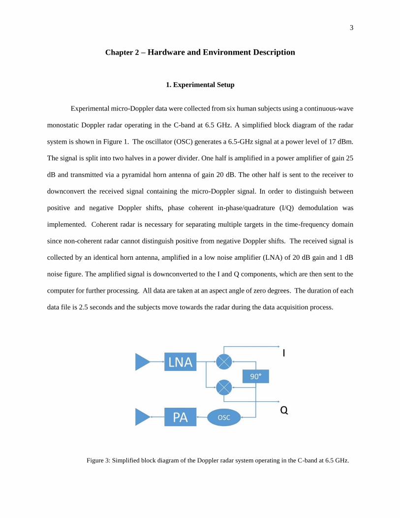
Experimental micro-Doppler data were collected from six human subjects using a continuous-wave
monostatic Doppler radar operating in the C-band at 6.5 GHz. A simplified block diagram of the radar
system is shown in Figure 1. The oscillator (OSC) generates a 6.5-GHz signal at a power level of 17 dBm.
The signal is split into two halves in a power divider. One half is amplified in a power amplifier of gain 25
dB and transmitted via a pyramidal horn antenna of gain 20 dB. The other half is sent to the receiver to
downconvert the received signal containing the micro-Doppler signal. In order to distinguish between
positive and negative Doppler shifts, phase coherent in-phase/quadrature (I/Q) demodulation was
implemented. Coherent radar is necessary for separating multiple targets in the time-frequency domain
since non-coherent radar cannot distinguish positive from negative Doppler shifts. The received signal is
collected by an identical horn antenna, amplified in a low noise amplifier (LNA) of 20 dB gain and 1 dB
noise figure. The amplified signal is downconverted to the I and Q components, which are then sent to the
computer for further processing. All data are taken at an aspect angle of zero degrees. The duration of each
data file is 2.5 seconds and the subjects move towards the radar during the data acquisition process.
Figure 3: Simplified block diagram of the Doppler radar system operating in the C-band at 6.5 GHz.
4
2. Environmental Description
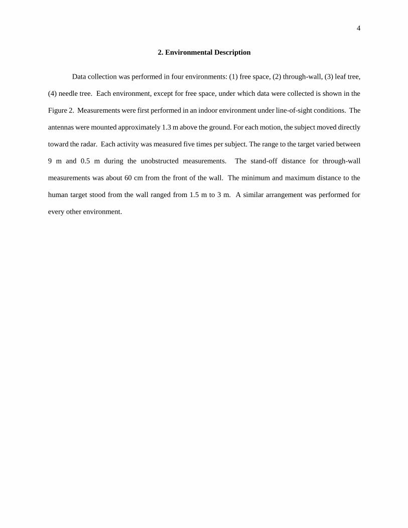
Data collection was performed in four environments: (1) free space, (2) through-wall, (3) leaf tree,
(4) needle tree. Each environment, except for free space, under which data were collected is shown in the
Figure 2. Measurements were first performed in an indoor environment under line-of-sight conditions. The
antennas were mounted approximately 1.3 m above the ground. For each motion, the subject moved directly
toward the radar. Each activity was measured five times per subject. The range to the target varied between
9 m and 0.5 m during the unobstructed measurements. The stand-off distance for through-wall
measurements was about 60 cm from the front of the wall. The minimum and maximum distance to the
human target stood from the wall ranged from 1.5 m to 3 m. A similar arrangement was performed for
every other environment.

5
(a)
(b)
(c)
Figure 4: Experimental setup in each environment: (a) through-the-wall, (b) leaf tree foliage, (c) and needle tree
foliage.
There was a non-negligible wind blowing in the course of outdoor data collection for leaf and
needle tree foliage. This wind factor was characterized by intermittent wind bursts of up to 5–10 mph
which caused relatively greater noise in the received signal for needle tree data. Wind at this speed is
particularly problematic because it is at the same speed typical of human movements of walking and

6
jogging. The wind is definitely an important factor that can affect the classification rate for through-foliage
clutter, which is observed in the relatively large misclassification rate for needle tree foliage shown later in
this thesis.
3. Time-frequency analysis:
The goal of time-frequency analysis is to detect what frequencies are present in a signal, how strong
they are, and how they change over time. The study of signals with time-varying frequency content has
motivated the development of large array time-frequency representations (TFRs). Conventional signal
processing tools, such as the Fourier transform, are unsuitable for signals that contain time-varying
frequency content and thus other tools for analysis must be sought. For the purposes of micro-Doppler
signal analysis, it is not enough to only know what frequencies are present in the received signal. The
theory behind common TFRs along with their application to non-stationary synthetic data will be examined
below. The four TFRs utilized are the short-time Fourier transform, wavelet transform, Wigner-Ville
distribution, and the Hilbert Huang transform. The properties of each transform, along with merits and
demerits of each time-frequency transformation on the synthetic data, will be discussed.
3.1 Short-time Fourier transform
The short-time Fourier transform (STFT) is a linear TFR useful for analyzing piece-wise stationary
signals. It is composed of two steps: first, the signal is divided into two time segments and then the spectrum
of each segment is obtained via the Fourier transform. This procedure results in 3D representation which
displays the evolution of frequency content over time. Mathematically, it is expressed by the following
equation:
STFT(𝑡, 𝑓) = ∫ 𝑥(𝜏)ℎ∗(+∞
−∞
𝜏 − 𝑡)𝑒−𝑗2𝜋𝑓𝜏𝑑𝜏
where ℎ(𝑡) is the time-window centered at 𝑡 = 0 which is used to extract time segments. The requires
the window to have unit energy:

7
∫ |ℎ(𝑡)|2𝑑𝑡 = 1+∞
−∞
The STFT is the most popular TFR and because it has low computational complexity and is simple
to implement. The STFT is limited by the Gabor-Heisenberg uncertainty principle: resolution in time and
frequency cannot be made arbitrarily small simultaneously.
∆𝑡∆𝑤 ≥ 1
2
Thus, an inherent limitation for joint time-frequency resolution exists for the STFT. As the length
of the window increases, time-resolution is lost and frequency-resolution is gained. As the length of the
window decreases, time-resolution is gained while frequency-resolution is lost.
3.2 Continuous Wavelet transform
The continuous wavelet transform (CWT) is a linear TFR obtained by decomposing a signal into
shifted and scaled versions of a mother wavelet. Mathematically, the CWT can be expressed as,
CWT(𝑡, 𝑎) = 1
√𝑎∫ 𝑥(𝜏)𝑤∗ (
𝜏 − 𝑡
𝑎)
+∞
−∞
𝑑𝜏
where 𝑎 is the scale and 𝑤(𝑡) is the mother wavelet. To obtain an admissible representation, 𝑤(𝑡) must
have zero-mean, i.e.
∫ 𝑤(𝑡)𝑑𝑡 = 0+∞
−∞
The most common mother wavelets are Mexican-Hat, Morlet, or Daubechies wavelets. The CWT,
leads to a time-scale representation since it displays the signal time-frequency evolution at different scales.
However, there is a direct correlation between scale and frequency. If the central frequency of the mother
wavelet 𝑤(𝑡) is𝑓0, the scale 𝑎 corresponds to the frequency 𝑓 = 𝑓0/𝑎. In contrast to the STFT, the CWT
is a multi-resolution technique that favors time-resolution at high-frequency and the frequency-resolution
at low-frequencies.

8
3.3 Wigner-Ville distribution
Unlike the previous two TFRs, the Wigner-Ville distribution (WVD) focuses on the decomposition
of the signal energy in the time-frequency plane as opposed to decomposition of the signal itself. The WVD
is expressed mathematically as follows,
WVD(𝑡, 𝑓) = ∫ 𝑥 (𝑡 +𝜏
2) 𝑥∗ (𝑡 −
𝜏
2)
+∞
−∞
𝑒−𝑗2𝜋𝑓𝜏𝑑𝜏
The WVD is not constrained by the Heisenberg-Gabor inequality. However, the nonlinearity of
the WVD introduces cross-term interference. These interference terms can render the time-frequency
representation difficult to interpret. To reduce this interference, the analytic signal of the input signal is
usually analyzed instead of the signal itself.
3.4 Hilbert-Huang Transform
The Hilbert-Huang transform (HHT) is a signal analysis method specifically designed to fill the
void for analysis nonlinear and non-stationary data. Unlike the previous methods, HHT is data-driven,
which means that it does not use a priori basis functions and instead adapts to the signal. The HHT is
composed of two parts: empirical mode decomposition (EMD) and Hilbert spectral analysis (HSA).
The EMD process is as follows. First, the extrema (minima and maxima) of the signal are located
and connected via spline interpolation to form an envelope. The mean of this envelope is designated as 𝑚1
and then subtracted from the original signal, forming the proto-IMF, ℎ1 = 𝑥(𝑡) − 𝑚1. The same process
is then applied to the proto-IMF until the definition of an IMF has been satisfied. ℎ11 = ℎ1 − 𝑚11. This
sifting process is repeated 𝑘 times until ℎ1𝑘is an IMF, that is ℎ1𝑘 = ℎ1(𝑘−1) − 𝑚1𝑘 , thus the first IMF
component is obtained, i.e. IMF1 = ℎ1𝑘. Then separate IMF1 from the original times series by
𝑥(𝑡) − IMF1 = 𝑟1. Treat 𝑟1as the new data and subject it to the same sifting process as above. Repeat this
procedure on all the subsequent 𝑟𝑖s, i.e. 𝑟2 = 𝑟1 − IMF2, … , . 𝑟𝑛 = 𝑟𝑛−1 − IMF𝑛 . The final result is
𝑥(𝑡) = ∑ IMF𝑖(𝑡) + 𝑟𝑛(𝑡)
𝑛
𝑖=1

9
An IMF is defined by the following criterion:
1. In the whole dataset, the number of extrema and the number of zero-crossings must either equal
or differ at most by one.
2. At any point, the mean value of the envelope defined by the local maxima and the envelope
defined by the local minima is zero.
4. Characteristics of non-ideal I/Q demodulation:
To implement ideal I/Q demodulation, the following requirements must be satisfied:
The local oscillator and the transmitter must be identical
The I and Q channels must have perfectly matched transfer functions over the signal bandwidth
The oscillators used to demodulate the I and Q channels must be exactly in quadrature, that is, 90
degrees out of phase with one another
When these requirements are not met, the received signal does not only contain the desired signal
component (with a slightly modified amplitude), but also an image component with a different amplitude
and a conjugated phase function, as well as a complex DC term. The image component is an error resulting
from the amplitude and phase mismatches; the DC component is the direct result of the individual channel
DC offsets. A diagram depicting the differences between ideal and non-ideal I/Q demodulation is shown
below in Figure 2.
a. Correction of I and Q channel imbalances in the time-domain:
An approach to the correction of I and Q imbalance in the time-domain will now be presented.
The non-ideal effects of I/Q demodulation can be represented below by the following equations:
𝐼(𝑡) = Acos(𝑤𝑡 + 𝜑) + 𝑎
𝑄(𝑡) = 𝐴(1 + 𝜖)sin(𝑤𝑡 + 𝜑 + 𝜃) + 𝑏

10
where (1 + 𝜖) represents the amplitude imbalance between channels, 𝜃 represents the phase
imbalance between channels, and 𝑎 and 𝑏 represent the DC offset of each channel respectively.
After subtracting the DC offset, which is simply the mean value of the signal, the I and Q channels
become:
𝐼′(𝑡) = Acos(𝑤𝑡 + 𝜑)
𝑄′(𝑡) = 𝐴(1 + 𝜖)sin(𝑤𝑡 + 𝜑 + 𝜃)
To compensate for the amplitude and phase imbalance, the following matrix can be setup with the
error correction terms 𝑐 and 𝑑.
[𝐼′′(𝑡)
𝑄′′(𝑡)]= [
1 0c d
] [𝐼′(𝑡)
𝑄′(𝑡)]
𝑐 = − tan(𝜃)
𝑑 =1
(1 + 𝜖)cos (𝜃)
Unlike 𝐼(𝑡) and 𝑄(𝑡), 𝐼′′(𝑡) and 𝑄′′(𝑡) are exactly in quadrature with one another. The task now
is to actually relate the 𝑐 and 𝑑 terms to the physical signal at hand. After some derivations, it was shown
in Ref. X that the 𝑐 and 𝑑 terms can be solved for in the following manner:
𝑐 = − (𝐼, 𝑄)
𝑠𝑞𝑟𝑡( ‖𝐼‖2‖𝑄‖2 − (𝐼, 𝑄)2)
𝑑 = ‖𝐼‖2
𝑠𝑞𝑟𝑡( ‖𝐼‖2‖𝑄‖2 − (𝐼, 𝑄)2)

11
where (𝐼, 𝑄) represents the inner product operation and ‖𝐼‖ represents the norm of I. These correction
terms can now be processed to counteract the imbalance errors plaguing the I/Q system.

12
Chapter 3 – Comprehensive Data Display
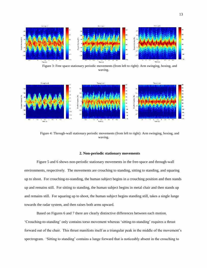
1. Periodic stationary movements
Figures 3 and 4 show typical MDS of the first three stationary movements in a free-space (FS)
and through-wall (TW) environment, respectively. They are arm swinging, boxing, and waving. For arm
swinging, the human subject stands still and swings his/her arms as if walking. For boxing, the human
subject alternates between right hand and left hand punches in the direction of the radar. For waving, the
human subject stands still and gestures back and forth in the direction facing the radar.
All motions have an average Doppler shift of 0 Hz, as expected, since the human is stationary.
What distinguishes each movement is the total Doppler spread, or total bandwidth, the swing rate, and the
sequence in which positive and negative frequency peaks occur. Waving has a smaller Doppler spread of
roughly 100 Hz of the three movements, while the other two have a total bandwidth of about 200 Hz. For
arm-swinging, positive and negative shifts occur simultaneously, whereas in the other movements, there
is a delay between the occurrence of one and the other. In other words, for arm swinging, the positive and
negative shifts occur ‘in parallel’ (simultaneously) but the positive and negative shifts in boxing and
waving occur ‘sequentially’ (one after the other). The overall structure of the signatures remains
unchanged for through-wall MDS, although the lower SNR is observed. Fading effects are not evident in
these signatures since they are stationary.
13
Figure 3: Free space stationary periodic movements (from left to right): Arm swinging, boxing, and
waving.
Figure 4: Through-wall stationary periodic movements (from left to right): Arm swinging, boxing, and
waving.
2. Non-periodic stationary movements
Figure 5 and 6 shows non-periodic stationary movements in the free-space and through-wall
environments, respectively. The movements are crouching to standing, sitting to standing, and squaring
up to shoot. For crouching-to-standing, the human subject begins in a crouching position and then stands
up and remains still. For sitting to standing, the human subject begins in metal chair and then stands up
and remains still. For squaring up to shoot, the human subject begins standing still, takes a single lunge
towards the radar system, and then raises both arms upward.
Based on Figures 6 and 7 there are clearly distinctive differences between each motion.
‘Crouching-to-standing’ only contains torso movement whereas ‘sitting-to-standing’ requires a thrust
forward out of the chair. This thrust manifests itself as a triangular peak in the middle of the movement’s
spectrogram. ‘Sitting to standing’ contains a lunge forward that is noticeably absent in the crouching to

14
standing case. ‘Squaring up to shoot’ involves the human target lunging forward and then raising both
arms toward the radar. It is very similar to ‘sitting to standing’ but one can also see the human raising
their arms, indicated by the vertical peak near the end of the signature. The motion ‘squaring up to shoot’
can be thought of as a sequence of two motions – lunging forward and then raising arms. Again, despite
the attenuation from free-space to through-wall environments, the overall structure of the MDS remains
unchanged. Fading effects are again not evident in these signatures since they are stationary.
Figure 5: Free space stationary non-periodic movements (from left to right): Crouching to standing, sitting
to standing, and squaring up to shoot.
Figure 6: Through-wall stationary non-periodic movements (from left to right): Crouching to standing,
sitting to standing, squaring up to shoot.

15
3. Object-free movements
Figure 7 and 8 shows object-free forward-moving movements in free-space and through-wall
environments, respectively. The movements are walking, walking with arms crossed, limping, and
crawling. For walking, the human subject begins at a distance of about 7.5 meters and walks toward the
radar. The same is the case for walking with arms crossed. For limping, the human subject walks toward
the radar while dragging one foot to simulate being wounded. For crawling, the human subject crawls in
a baby-like manner towards the radar.
Note how the stride rate is exaggerated for the limping motion as opposed to non-limping motion.
There is a noticeable dragging effect that occurs in limping which does not occur for any other walking
motion. Thus, extracting stride rate as a feature for classification may be useful to separate walking
motion from limping, which can potentially be used in a military context for detecting wounded persons.
The stride rate disappears for crawling and we notice a more-or-less flat Doppler shift with small arm
movements atop the main shift. Crawling is characterized by a small Doppler shift with periodic peaks
that indicate arm movement and it has the lowest Doppler shift of each movement. Each walking activity
has approximately the same torso Doppler frequency, as expected, which is about 50 Hz. This Doppler
shift corresponds to a speed of 1.15 m/s, which is how fast humans typically walk. Again, these MDS
signatures are nearly identical to their free-space counterparts, differing only in amplitude.
Fading effects are now obvious in the TW signatures. The change in RCS over the duration of
the MDS indicates fading and may yield insight into whether the target is approaching or receding from
the radar system. Besides the attenuation and fading from FS to TW, the overall structure of the MDS
remains unchanged in each environment.

16
Figure 7: Free-space forward-moving (starting from top-left and moving clockwise): Walking, walking
with arms crossed against chest, limping, crawling.
Figure 8: Free-space forward-moving (starting from top-left and moving clockwise): Walking, walking
with arms crossed against chest, limping, crawling.

17
4. Carrying an object
Figures 9 and 10 show movements for a human target walking toward the radar while holding the
following objects: cylindrical brick, weighted backpack, cell phone up to ear, and corner reflector. Each
movement consists of a human subject walking towards the radar in a casual manner while holding onto
some particular object.
Observe how walking with the corner reflector emphasizes the torso movement of the human
subject. The corner reflector can be used as a surrogate for any object with a high RCS that may be
carried by a human target. A feature that measures the ratio of the torso amplitude to the arm/leg
amplitude may be used to discriminate regular walking from walking with an object with a high RCS.
Observe how walking with the cell phone eliminates the arm movement of one arm (the arm which is
holding the phone up to the ear), but movement of one arm is still visible. Walking while holding the
brick has a similar spectrogram with the walking case, but it has a slightly narrower frequency spread. In
general, carrying different objects does not make a noticeable difference in the spectrograms here except
for the corner reflector. Besides the attenuation and fading from FS to TW, the overall structure of the
MDS remains unchanged in each environment. Fading effects are now obvious in the TW signatures.

18
Figure 9: Free space forward moving while carrying an object (starting from top-left moving clockwise):
Walking with brick, walking with backpack, holding phone up to ear, corner reflector.
Figure 10: Through-wall forward-moving while carrying an object (starting from top-left moving
clockwise): Walking with brick, walking with backpack, walking with phone up to ear, walking with corner
reflector.

19
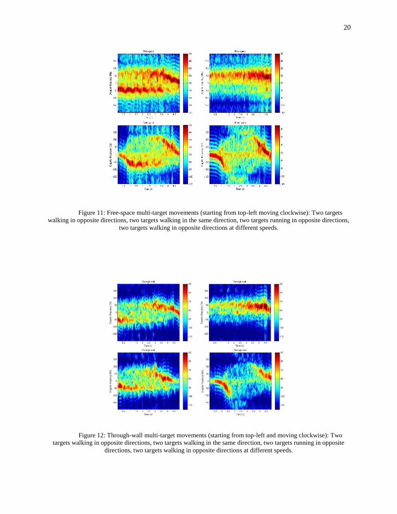
5. Multi-target movements
Figures 11 and 12 show multi-target movements in free-space and through-wall environments,
respectively. The movements are two targets walking in opposite directions, two targets walking towards
the radar, two targets running in opposite direction, and two targets walking in the opposite direction at
different speeds.
Multi-target movements present a challenge because the presence of several people
simultaneously in the radar field of sight could involve interferences. From the figures, we can see that it
is possible to separate multiple targets that are walking in opposite directions if the total bandwidth of
each target’s movement does not interfere with the other. If multiple targets are walking in the same
direction, however, the multiple targets will appear as one target. It gives no indication at all that there
are multiple targets on the scene. Fading effects are present in both the free-space and through-wall
MDS. Total Doppler bandwidth may be useful for distinguishing two targets. Doppler frequencies
would thus be mixed and the received signal could not be easily separated anymore. It was found that
while through-wall propagation affected the magnitude response of the Doppler spectrogram in the form
of attenuation and fading, it only introduced very minor distortions on the actual Doppler frequencies
from the body parts. Besides the attenuation and fading from FS to TW, the overall structure of the MDS
remains unchanged in each environment.
20
Figure 11: Free-space multi-target movements (starting from top-left moving clockwise): Two targets
walking in opposite directions, two targets walking in the same direction, two targets running in opposite directions,
two targets walking in opposite directions at different speeds.
Figure 12: Through-wall multi-target movements (starting from top-left and moving clockwise): Two
targets walking in opposite directions, two targets walking in the same direction, two targets running in opposite
directions, two targets walking in opposite directions at different speeds.

21
6. Variability across human subjects
The degree of variability in MDS across subjects depends on the movement being performed.
Table 1 lists the height and weight of the human subjects on whom data was collected. For movements
that only consist of arm movements such as stationary arm swinging or waving there tend to be less
variability across subjects than movements that involve the whole body such as crawling. Height and
weight have a greater impact on the MDS for movements that involve the entire body than they do for
stationary movements. Figures 13 and 14 show the variability of human MDS across different subjects
for stationary arm swinging and crawling, respectively. Despite there being slight variations in the MDS
across subjects for stationary arm swinging, the overall structure of the MDS remains the same. Some of
the heavier subjects give greater torso responses which can be seen from the increased amplitude in the
MDS – compare the torso response of heavier subject (subject 6) with that of a lighter subject (subject 5).
Unlike stationary arm swing, there appear to be significant structural changes in crawling across subjects.
Some subjects have a more uniform and periodic crawl (subjects 1 and 5) than the others (subjects 3 and
6). Thus it is important to recognize what features remain the same across subjects when designing
classifiers.
TABLE 1: PHYSICAL CHARACTERISTICS OF HUMAN SUBJECTS
Subject Identifier Height (m) Weight (kg)
1 1.73 68
2 1.83 74
3 1.55 54
4 1.75 58
5 1.93 102
6 1.72 77

22
Figure 13: Stationary arm swinging MDS across subjects (from top left going clockwise): Subjects 1, 3, 5,
and 6
Figure 14: Crawling MDS across subjects (from top left going clockwise): Subjects 1, 3, 5, and 6
23
In this thesis, we present the radar MDS of various human activities in free-space and through-
wall environments. The spectrograms show rather interesting and distinct signatures depending on the
activity.
The following experiments were used to analyze the different effects due to through-wall
transmission on human MDS. It was found that while through-wall propagation affected the magnitude
response of the Doppler spectrogram in the form of attenuation and fading, it only introduced very minor
distortions on the actual Doppler frequencies from the body parts. We also see that it is possible to
separate multiple targets that are moving in opposite directions under the proper circumstances. If the
targets are moving at different speeds, then they can be separated no matter what direction each target is
heading towards. But multiple targets can only be separated when they are traveling in the same direction
at different speeds. This may change significantly depending on aspect angle since a target at oblique
incidence only gives a radial component velocity which may cause the appearance of the target to be
slower than it actually is.
The extracted feature values are listed in Tables 2 and 3 for free space and through-wall scenarios,
respectively. The mean and the ±1 standard deviation values for each feature are shown. The standard
deviations account not only for the variability within each subject but also the variability between different
subjects. It is observed that the selected features for each activity are mostly consistent under both free
space and through-wall scenarios, although a few cases show significant differences. The differences may
be possibly be attributed the effects of multiple scattering between the human and the back surface of the
wall. We believe that these feature values would be useful in classification of human activities using radar
micro-Doppler signatures. While our derived features are based upon a 6.5-GHz transmit frequency, the
feature values indicated in Tables 3 and 4 can be scaled to other transmit frequencies since the Doppler
frequency is generally proportional to the actual transmit frequency. For example, we obtained a mean
cadence frequency (Feature 5) value of 1.231 Hz for walking (see Table 3), which when scaled from our
transmit frequency of 6.5 GHz to a 10.525-GHz transmit frequency comes to 1.993 Hz ( 5.6525.10231.1
). This value is virtually identical to a cadence frequency of 2 Hz obtained using a 10.525-GHz system in

24
Ref. 15. Similarly, the mean value of the average Doppler frequency (Feature 1), 66.812 Hz, for walking,
when scaled to a transmit frequency of 2.4 GHz is computed as 24.669 Hz ( 5.64.2812.66 ), which is
quite close to the value of 22.43 Hz listed in Ref. 16.

25
TABLE 2: LIST OF FEATURES USEFUL FOR FREE SPACE HUMAN ACTIVITY CLASSIFICATION
Activity
Mean
Doppler
frequency
(Hz)
Total
bandwidth
(Hz)
Doppler
offset (Hz)
Bandwidth
without MDS
(Hz)
Cadence
frequency
(Hz)
Period (Hz)
Stationary arm swinging 0.842 ± 0.433
270.142 ±
12.452
10.452 ±
3.465
75.642 ±
15.354
- 2.413 ± 1.814
Stationary boxing 1.246 ± 0.422
250.148 ±
16.538
15.321 ±
4.841
150.314 ±
20.003 - 7.165 ± 2.719
Stationary waving 1.184 ± 0.321
184.174 ±
6.910 6.321 ± 2.356 14.395 ± 3.516 - 5.234 ± 2.243
Sitting to standing 1.743 ± 0.456 80.214 ± 8.382 2.143 ± 0.423 2.546 ± 1.613 - -
Crouching to standing 3.412 ± 1.321 40.364 ± 6.290 3.141 ± 1.114 3.134 ± 2.212 - -
Squaring up to shoot 3.417 ± 0.423 120.124 ±
10.103
16.475 ±
2.428
15.243 ± 4.901 - -
Walking
66.812 ±
12.301
59.330 ± 9.776
60.412 ±
12.345
29.741 ± 4.246 1.231 ± 0.421 -
Walking with arms crossed
against chest
64.812 ±
11.325
61.798 ±
10.484
57.146 ±
11.934
30.265 ± 6.348 1.178 ± 0.158 -
Limping
34.013 ±
10.290 72.829 ± 7.298
30.142 ±
4.912 35.841 ± 3.385 1.012 ± 0.612 -
Crawling 18.394 ± 3.621 30.061 ± 4.737
39.647 ±
5.329 15.234 ± 2.458 1.574 ± 0.738 -
Walking with brick 61.174 ± 6.427 58.214 ± 8.406 30.987 ±
3.235
25.145 ± 5.243 4.176 ± 1.184 -
Walking with corner reflector 62.346 ± 5.294 58.997 ±
11.191
29.326 ±
2.195
24.147 ± 6.921 5.174 ± 1.253 -
Walking with backpack 64.184 ± 3.219
60.321 ±
12.348
28.244 ±
2.612
31.364 ± 7.365 4.967 ± 1.285 -
Walking with phone up to ear 65.174 ± 2.486
62.479 ±
13.348
28.471 ±
2.421 32.022 ± 6.388 5.037 ± 1.732 -

26
TABLE 3: LIST OF FEATURES USEFUL FOR THROUGH-WALL HUMAN ACTIVITY CLASSIFICATION
Activity
Mean
Doppler
frequency
(Hz)
Total
bandwidth
(Hz)
Doppler
offset (Hz)
Bandwidth
without
MDS (Hz)
Cadence
frequency
(Hz)
Period (Hz)
Stationary arm swinging 0.921 ±0.246
275.234 ±
20.285
12.234 ±
2.391
77.453 ±
6.556
- 3.012 ± 1.423
Stationary boxing 2.731 ± 1.575
247.831 ±
19.234
16.313 ±
5.728
148.212 ±
18.299 - 6.621 ± 3.718
Stationary waving 1.913 ±1.325
186.322 ±
16.264 8.493 ± 3.199
15.321 ±
1.642 - 6.120 ± 2.914
Sitting to standing 1.621 ± 1.925 78.183 ±
8.345
3.348 ± 2.341 2.857 ± 1.243 - -
Crouching to standing 4.136 ± 2.539
43.312 ±
14.429
2.912 ± 1.824 2.821 ± 1.845 - -
Squaring up to shoot 2.891 ± 1.056
117.233 ±
18.924
18.183 ±
4.516
18.341 ±
3.533
- -
Walking
63.682 ±
8.195
57.385 ±
8.165
63.532 ±
12.324
25.134 ±
6.569
1.779 ± 0.349 -
Walking with arms crossed against
chest
67.062 ±
6.244
55.527 ±
5.404
58.283 ±
5.002
27.436 ±
4.013 1.112 ± 0.806 -
Limping 35.431 ±
8.294
70.737 ±
5.686
27.345 ±
4.208
35.213 ±
4.830
2.119 ± 1.429 -
Crawling 17.635 ±
3.565
24.357 ±
4.380
40.122 ±
11.123
20.038 ±
3.234
3.394 ± 2.544 -
Walking with brick
63.677 ±
7.341
62.481 ±
11.121
30.421 ±
4.348
32.356 ±
7.659
5.120 ± 2.890 -
Walking with corner reflector
60.069 ±
8.294
61.238 ±
9.824
29.123 ±
2.142
30.212 ±
4.592 6.496 ± 1.435 -
Walking with backpack
65.312 ±
7.345
62.219 ±
7.365
28.314 ±
5.429
31.313 ±
4.492 5.712 ± 1.233 -
Walking with phone up to ear 64.213 ±
8.214
57.186 ±
4.233
29.313 ±
7.643
28.213 ±
3.329
6.010 ± 1.276 -
27
7. Human gait micro-Doppler signature database
Human gait micro-Doppler signature database
The spectrograms shown below represent the beginning of an attempt to build a database of
human gait MDS. We plan to fill this database with over 100 movements for multiple human subjects.
These movements may be classified into categories such as fundamental gait movements, transition
movements, communicative hand gestures, common warfare movements, and so on. Examples of
“fundamental gait movements” may include a single step towards the radar or a single arm-swing cycle
while examples of “transition movements” may include crouching-to-standing or standing-to-sitting in a
chair. In future research, we will think of ways to discriminate signatures. In this report however we will
only display the signatures.
The following MDS shown in Figures 15-43 were recorded for a wide variety of activities in an
outdoor environment using a continuous-wave X-band radar system operating at 6.5 GHz. The
spectrogram is used simply because it is convenient to implement and gives a good rough overview of the
signature. The optimal time-frequency representation for classification of human gait MDS is still a topic
we are pursuing. All the signatures shown below were taken from subject #2 from Table 1.

28
Figure 15: MDS of stationary human standing still (breathing) in free space.
Figure 16: MDS of human standing still and breathing heavily in free space.

29
Figure 17: MDS of human standing still and holding breath in free space.
Figure 18: MDS of sitting in chair breathing heavily.
30
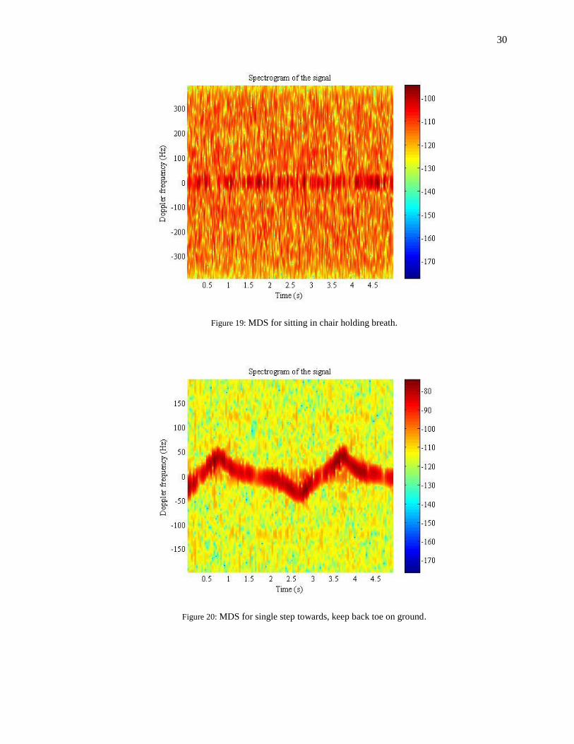
Figure 19: MDS for sitting in chair holding breath.
Figure 20: MDS for single step towards, keep back toe on ground.

31
Figure 21: MDS for single step towards, bring both feet together.
Figure 22: MDS for two steps toward, keep back toe on ground.

32
Figure 23: MDS for right arm swing cycle.
Figure 24: MDS for left arm swing cycle.

33
Figure 25: MDS for both arm swing cycle, same direction.
Figure 26: MDS for both arm swing cycle, opposite direction.

34
Figure 27: MDS for raise right arm forward once.
Figure 28: MDS for raise left arm forward once.

35
Figure 29: MDS for raise both arms forward once at same time.
Figure 30: MDS of raise both arms forward once at different time.

36
Figure 31: MDS for oscillate between raising left and right arm.
Figure 32: MDS for single right hand punch towards starting at boxing position.

37
Figure 33: MDS of single left hand punch towards starting at boxing position.
Figure 34: MDS of single punch both hands starting at boxing position.

38
Figure 35: MDS of punch while oscillating between hands.
Figure 36: MDS of turning around, facing towards.
39
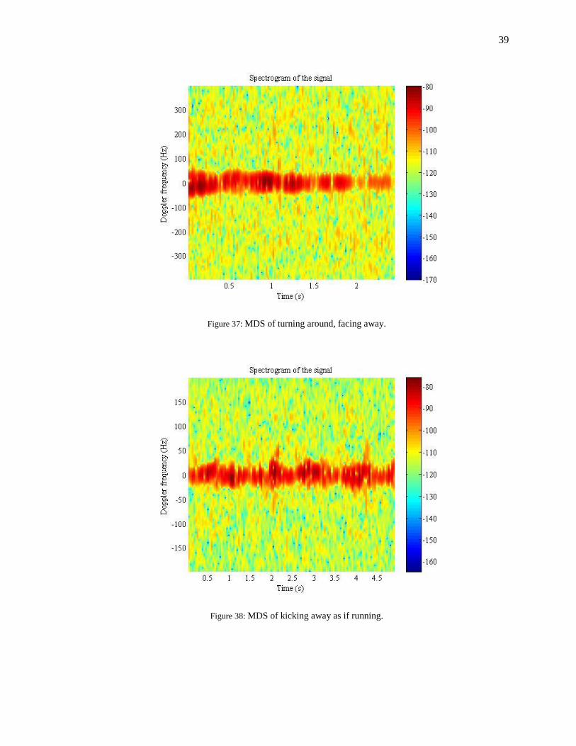
Figure 37: MDS of turning around, facing away.
Figure 38: MDS of kicking away as if running.
40
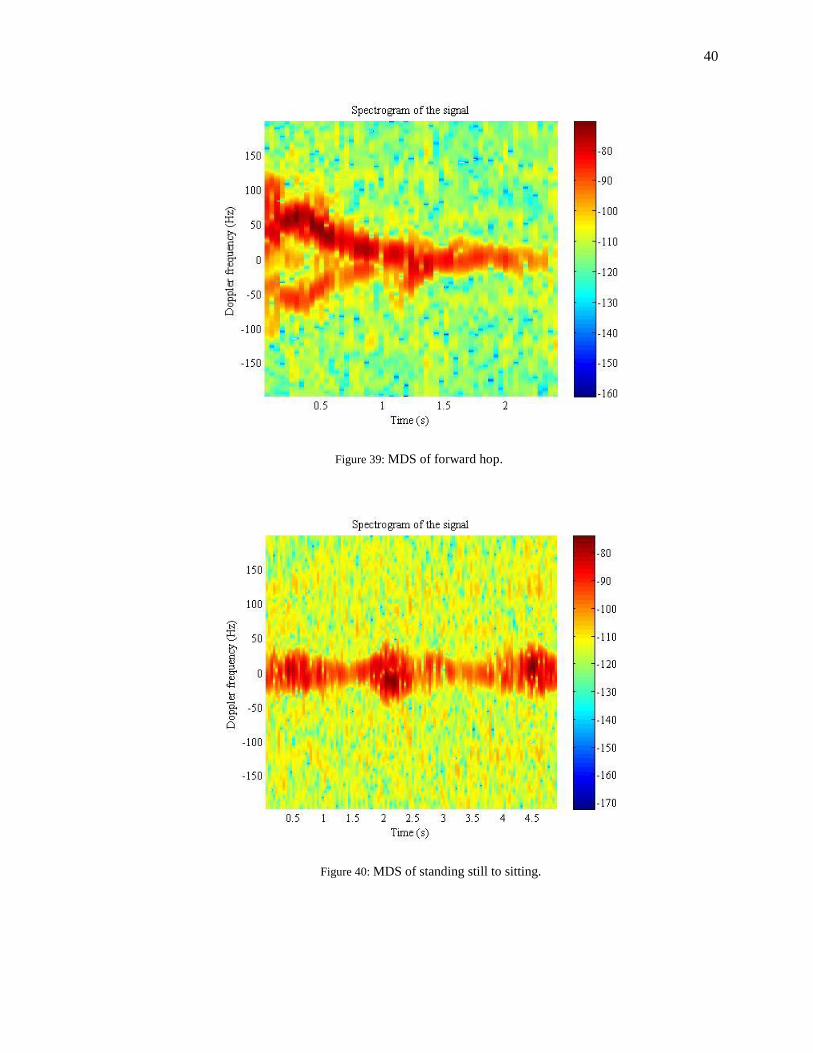
Figure 39: MDS of forward hop.
Figure 40: MDS of standing still to sitting.

41
Figure 41: MDS of standing still to crouching.
Figure 42: MDS of walking towards and stopping.

42
Figure 43: MDS of sitting to standing still.
43
Chapter 4 – Feature Extraction and Classification
1. Feature extraction
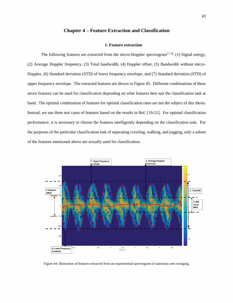
The following features are extracted from the micro-Doppler spectrogram17,18: (1) Signal energy,
(2) Average Doppler frequency, (3) Total bandwidth, (4) Doppler offset, (5) Bandwidth without micro-
Doppler, (6) Standard deviation (STD) of lower frequency envelope, and (7) Standard deviation (STD) of
upper frequency envelope. The extracted features are shown in Figure 45. Different combinations of these
seven features can be used for classification depending on what features best suit the classification task at
hand. The optimal combination of features for optimal classification rates are not the subject of this thesis.
Instead, we use three test cases of features based on the results in Ref. [19-21]. For optimal classification
performance, it is necessary to choose the features intelligently depending on the classification task. For
the purposes of the particular classification task of separating crawling, walking, and jogging, only a subset
of the features mentioned above are actually used for classification.
Figure 44: Illustration of features extracted from an experimental spectrogram of stationary arm swinging.

44
To compare the distribution of features across environments, scatter graphs of features from each
environment are presented in Figure 46. Table 4 shows the numeric distribution of all extracted features
using the mean and standard deviation. The feature space displayed in these graphs does not represent the
actual features used in our classifier.
(a)
(b)
(c)
(d)
Figure 45: Two-dimensional un-normalized feature space comparison for each environment: (a) free-space, (b) through-the-wall,
(c) leaf tree foliage, and (d) needle tree foliage. The feature along the x-axis is mean Doppler frequency while the feature along
the y-axis is the total bandwidth.

45
The feature statistics are shown across environment in Table 4. This table includes all 7 features
extracted from the spectrogram. The increase in standard deviation indicates the noise added in both the
outdoor foliage environments and through-the-wall. This spread in standard deviation is representative
for crawling and jogging as well, but out of interest of space we chose to only include a table for walking.
There is a significant increase in the standard deviation for outdoor tree foliage. The standard deviations
are included. The standard deviation shows how much the average. There is no big increase in Doppler
offset, or in the standard deviation. There is a very large increase for bandwidth, however.
TABLE 4: COMPARISON OF FEATURE STATISTICS FOR WALKING MOTION ACROSS DIFFERENT
ENVIRONMENTS
Environment Energy
(arbitrary
units)
Avg.
Doppler
(Hz)
Total BW
(Hz)
Doppler
offset
(Hz)
BW without
MDS
(Hz)
STD lower
(Hz)
STD upper
(Hz)
Free space 3.157
±
2.482
42.445
±
4.653
154.659
±
20.016
46.247
±
14.347
66.465
±
13.422
53.918
±
12.649
34.423
±
7.316
Through-the-
wall
0.074
±
0.059
29.327
±
3.951
120.980
±
20.290
40.880
±
15.275
35.454
±
25.516
45.640
±
10.740
44.812
±
15.548
Needle tree
foliage
0.046
±
0.114
15.520
±
15.408
203.498
±
47.497
35.805
±
17.222
116.306
±
33.701
44.849
±
19.274
48.414
±
20.761
Leaf tree foliage 0.019
±
0.039
20.877
±
19.985
201.809
±
42.909
33.746
±
12.359
128.292
±
33.835
35.679
±
10.121
40.964
±
15.977
46
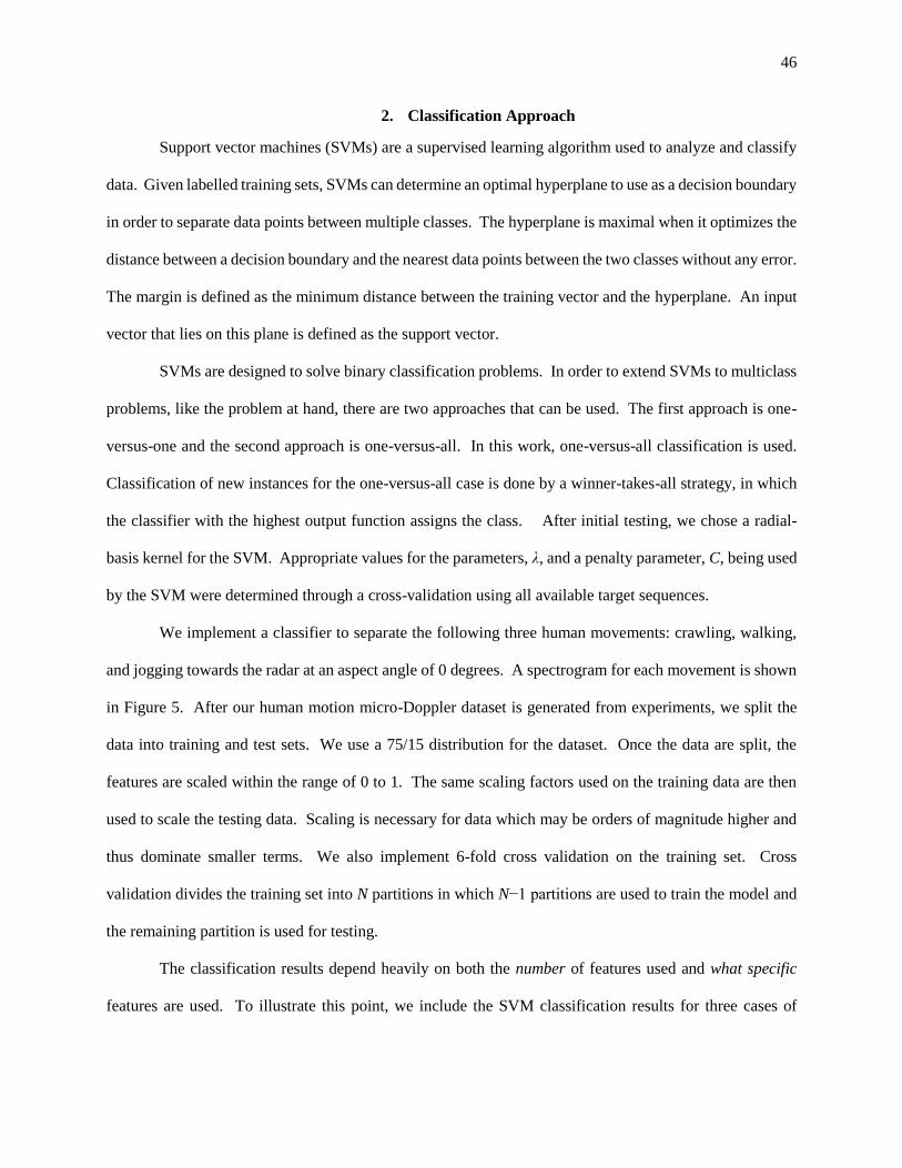
2. Classification Approach
Support vector machines (SVMs) are a supervised learning algorithm used to analyze and classify
data. Given labelled training sets, SVMs can determine an optimal hyperplane to use as a decision boundary
in order to separate data points between multiple classes. The hyperplane is maximal when it optimizes the
distance between a decision boundary and the nearest data points between the two classes without any error.
The margin is defined as the minimum distance between the training vector and the hyperplane. An input
vector that lies on this plane is defined as the support vector.
SVMs are designed to solve binary classification problems. In order to extend SVMs to multiclass
problems, like the problem at hand, there are two approaches that can be used. The first approach is one-
versus-one and the second approach is one-versus-all. In this work, one-versus-all classification is used.
Classification of new instances for the one-versus-all case is done by a winner-takes-all strategy, in which
the classifier with the highest output function assigns the class. After initial testing, we chose a radial-
basis kernel for the SVM. Appropriate values for the parameters, λ, and a penalty parameter, C, being used
by the SVM were determined through a cross-validation using all available target sequences.
We implement a classifier to separate the following three human movements: crawling, walking,
and jogging towards the radar at an aspect angle of 0 degrees. A spectrogram for each movement is shown
in Figure 5. After our human motion micro-Doppler dataset is generated from experiments, we split the
data into training and test sets. We use a 75/15 distribution for the dataset. Once the data are split, the
features are scaled within the range of 0 to 1. The same scaling factors used on the training data are then
used to scale the testing data. Scaling is necessary for data which may be orders of magnitude higher and
thus dominate smaller terms. We also implement 6-fold cross validation on the training set. Cross
validation divides the training set into N partitions in which N−1 partitions are used to train the model and
the remaining partition is used for testing.
The classification results depend heavily on both the number of features used and what specific
features are used. To illustrate this point, we include the SVM classification results for three cases of

47
features. The classification results for different feature spaces are shown here. There are three cases of
features investigated:
Case 1: (1) Average Doppler frequency, (2) Total bandwidth
Case 2: (1) Doppler offset, (2) Bandwidth without MDS, (3) Total bandwidth
Case 3: (1) Average Doppler frequency, (2) Total bandwidth, (3) Doppler offset, (4) Bandwidth without
MDS.
Figure 46: Spectrograms of three different types of human motions in the free-space environment: (a) crawling, (b) walking, and
(c) jogging.
It is not known a priori which set of features will result in the highest classification rate and
therefore they must be experimentally determined. However, it was shown in other works that the most
effective features were the torso frequency, total bandwidth, Doppler offset, and bandwidth without MDS,
which result in the greatest separability for moving human targets5. It was also shown that the classification
rate increases asymptotically as the number of features increases.

48
3. Classification Results
We train a Support Vector Machine (SVM) with the feature vectors mentioned in Section 4.1 using
a radial basis kernel (RBF). We then validate the classifier’s accuracy on unused data (i.e., not used in the
training) and observe the classification results, which are shown below in Table 2. The features introduced
in Section 3 are extracted from the measured spectrograms.
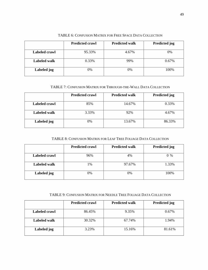
An accessible format for the results of classification is the confusion matrix. The features used are
the same as the features for Case 3. These features were used since they gave the highest classification rate
across the board for each environment, as can be seen in Table 5. Confusion matrices are shown in Tables
6-9 for each data collection environment averaged over 10 iterations.
TABLE 5: SVM CLASSIFICATION RATE (10 ITERATIONS): 75/15 SPLIT
Features
used
Free
space
Through-
the-wall
Leaf
tree foliage
Needle
tree foliage
Case 1 86.00% 72.22% 83.56% 53.88%
Case 2 89.44% 77.44% 88.00% 80.63%
Case 3 98.11% 87.78% 97.89% 81.12%
For this particular classification task, free space gave the highest classification rate at 98.11%. The
second best classification task occurs for leaf tree foliage at 97.89%. The classification rates are highest
for the data collection in free space, as one would expect. Due to windy conditions for needle tree data
collection, the classification rates were the lowest. The importance of the number of features can be seen
here since for Case 1, the classification rate for needle tree data is very low but significantly increases as
the number of features used increases for Case 2 and 3. A wind factor resulted in consistently higher
misclassification rates for the needle tree. It is shown that increasing the number of features generally
increases the classification rate as well. And in windy conditions it can be seen that for two features (Case
1), the needle tree classifier is almost unusable at 46% classification accuracy.
49
TABLE 6: CONFUSION MATRIX FOR FREE SPACE DATA COLLECTION
Predicted crawl Predicted walk Predicted jog
Labeled crawl 95.33% 4.67% 0%
Labeled walk 0.33% 99% 0.67%
Labeled jog 0% 0% 100%
TABLE 7: CONFUSION MATRIX FOR THROUGH-THE-WALL DATA COLLECTION
Predicted crawl Predicted walk Predicted jog
Labeled crawl 85% 14.67% 0.33%
Labeled walk 3.33% 92% 4.67%
Labeled jog 0% 13.67% 86.33%
TABLE 8: CONFUSION MATRIX FOR LEAF TREE FOLIAGE DATA COLLECTION
Predicted crawl Predicted walk Predicted jog
Labeled crawl 96% 4% 0 %
Labeled walk 1% 97.67% 1.33%
Labeled jog 0% 0% 100%
TABLE 9: CONFUSION MATRIX FOR NEEDLE TREE FOLIAGE DATA COLLECTION
Predicted crawl Predicted walk Predicted jog
Labeled crawl 86.45% 9.35% 0.67%
Labeled walk 30.32% 67.74% 1.94%
Labeled jog 3.23% 15.16% 81.61%

50
Chapter 5 – Conclusions
This thesis constitutes a preliminary study on how different radar environments can impact the
classification rate of human movements using radar micro-Doppler signatures. This study has shown that
the data collection environment certainly can have a large impact on human motion classification. It was
found that environments like free space and leaf tree foliage result in the highest classification rate while
environments like through-the-wall and needle tree foliage result in much lower classification rates. It can
be seen how the feature statistics change across environments and consequently the classification rate as
well.
Some suggestions for future work may include the exploration of different features with respect to
aspect angle. It may be the case that some features are more robust with respect to changes in aspect angle
even though they result in less separable feature spaces at zero degree aspect angle (arm swing rate, for
instance). Another suggestion would be the testing of human movements in different weather conditions.

51
Bibliography
[1] Chen, V. C., Li, F., Ho, S.-S, and Wechsler, H., “Analysis of micro-Doppler signatures,” IEEE Proceedings -
Radar, Sonar and Navigation 150(4), 271-276 (2003).
[2] Serir, A., and Bouhafsi Y., “Micro-doppler radar signature classification by time-frequency and time-scale
analysis,”
in [Proc. 11th International Conference on Information Sciences, Signal Processing and their Applications
(ISSPA)], Montreal, QC, 995-1000 (July 2012).
[3] Karabacak, C., Gurbuz, S. G., Gurbuz, A. C., Guldogan, M. B., Hendeby, G., and Gustafsson, F., “Knowledge
exploitation for human micro-Doppler classification,” IEEE Geoscience and Remote Sensing Letters 12(10),
2125-2129 (2015).
[4] Tivive, F. H. C., Phung, S. L, and Bouzerdoum, A. “An image-based approach for classification of human micro-
Doppler radar signatures,” in [Proc. SPIE Conference on Active and Passive Signatures IV], Baltimore, MD,
873406-1-873406-12 (April 2013).
[5] Alemdaroğlu, Ö. T., Candan, Ç., and Koç, S., “The radar application of micro Doppler features from human
motions,” in [Proc. IEEE Radar Conference (RadarCon)], Arlington, VA, 374-379 (May 2015).
[6] Chen, V.C., Li, F., Ho, S.-S, and Wechsler, H., “Analysis of micro-Doppler signatures,” IEEE Proceedings -
Radar, Sonar and Navigation 150, 271-276 (2003).
[7] Chen, V.C., “Doppler signatures of radar backscattering form objects with micro-motion,” IET Signal
Processing 2, 291-300 (2008).
[8] Tahmoush, D., and Silvious, J. (2009). “Angle, elevation, PRF, and illumination in radar microDoppler for
security applications” in [Proc. IEEE Antennas and Propagation Society International Symposium (APSURSI
ʹ09)], Charleston, SC, 1-4 (2009).
[9] Ram, S.S., and Ling, H. (2008). “MicroDoppler signature simulation of computer animated and animal motions,”
in [Proc. IEEE Antennas and Propagation Society International Symposium (APS 2008)], San Diego, CA, 1-4,
(2008).
[10] Kim, Y., Ha, S., and Kwon, J., “Human detection using Doppler radar based on physical characteristics of
targets,” IEEE Geoscience and Remote Sensing Letters 12, 289-293 (2015).
[11] Liu, X., Leung, H., and Lampropoulos, G. A., “Effects of non-uniform motion in through-the-wall SAR
imaging,” IEEE Transactions on Antennas and Propagation 57(11), 3539-3548 (2009).
[12] Ram, S. S., Christianson, C., Kim, Y., and Ling, H., “Simulation and analysis of human micro-Dopplers in
through-wall environments,” IEEE Transactions on Geoscience and Remote Sensing 48(4), 2015-2023 (2010).
[13] Li, J., Zeng, Z., Sun, J., and Liu, F., “Through-Wall detection of human being’s movement by UWB Radar,”
IEEE Geoscience and Remote Sensing Letters 9(6), 1079-1083 (2012).
[14] Narayanan, R. M. and Zenaldin, M., “Radar micro-Doppler signatures of various human activities,” IET Radar,
Sonar & Navigation 9(9), 1205-1215 (2015).
[15] Garcia-Rubia, J. M., Kilic, O., Dang, V., Nguyen, Q., and Tran, N., “Analysis of moving human micro-Doppler
signature in forest environments,” Progress in Electromagnetics Research 148, 1-14 (2014).
[16] Anderson, M.G., [Design of Multiple Frequency Continuous Wave Radar Hardware and Micro-Doppler Based
Detection and Classification Algorithms], Ph.D. Dissertation, University of Texas at Austin (2008).
[17] Björklund, S., Petersson, H., Nezirovic, A., Guldogan, M.B., and Gustafsson, F. (2011). “Millimeter-wave radar
micro-Doppler signatures of human motion,” in [Proceedings of the International Radar Symposium (IRS)],
Leipzig, Germany, 167-174 (2011).
[18] Zhang, J., “Analysis of human gait radar signal using reassigned WVD,” Physics Procedia 24, 1607-1614
(2012).
[19] Zhang, J., “Basic gait analysis based on continuous wave radar,” Gait & Posture 36, 667-671 (2012).
[20] Li, F., Huang, B., Zhang, H., Du, H. (2012). “Human gait recognition using micro-Doppler features,” in [Proc.
5th Global Symposium on Millimeter Waves (GSMM)], Harbin, China, 326-329 (2012).
[21] Otero, M. (2005). “Application of a continuous wave radar for human gait recognition,” in [Proc. SPIE
Conference on Signal Processing, Sensor Fusion, and Target Recognition XIV], Orlando, FL, 538-548 (2005).