characteristics of vlf atmospherics near the resonance

Ann. Geophys., 28, 193–202, 2010www.ann-geophys.net/28/193/2010/© Author(s) 2010. This work is distributed underthe Creative Commons Attribution 3.0 License.

AnnalesGeophysicae

Characteristics of VLF atmospherics near the resonance frequencyof the Earth-ionosphere waveguide 1.6–2.3 kHz by observations inthe auroral region

A. A. Ostapenko1, E. E. Titova1,2, A. P. Nickolaenko3, T. Turunen4, J. Manninen4, and T. Raita4

1Polar Geophysical Institute, Kola Scientific Centre of Russian Academy of Sciences, Apatity 184200, Russia2Space Research Institute, Russian Academy of Sciences, Profsoyuznaya str, 84/32, 117997, Moscow, Russia3Usikov Institute for Radio-Physics and Electronics, Nat. Acad. of Sciences of the Ukraine, 12, Acad. Proskura street,Kharkov 61085, Ukraine4Sodankyla Geophysical Observatory, Tahtelantie 62, 99600 Sodankyla, Finland

Received: 15 June 2009 – Revised: 3 November 2009 – Accepted: 30 November 2009 – Published: 20 January 2010

Abstract. Recordings of ELF-VLF waves with the right-hand (RH) and the left-hand (LH) circular polarization weremade in Northern Finland. Analysis showed a difference be-tween the RH and LH polarized waves. A pronounced max-imum of the wave amplitude was observed at the first crit-ical frequency of the Earth-ionosphere waveguide (the firsttransverse resonance) around 1.6–2.3 kHz. The wave had thecircular LH polarization at this maximum. To interpret ob-servations, we computed the characteristics of the waveguidemodes by using the full wave solution in the night model ofthe ionosphere. Computations show that the spectral maxi-mum at the first transverse resonance frequency arises from asmall absorption of the LH polarized radio wave in the mag-netized ionosphere plasma, forming the upper boundary ofthe Earth-ionosphere waveguide.

Keywords. Radio science (Radio wave propagation)

1 Introduction

Measurement of atmospherics (or sferics) is the moststraightforward way to study the ELF-VLF radio propagationin the Earth-ionosphere cavity. Signals originate from thelightning discharges and propagate over distances of a fewthousand kilometres owing to relatively small attenuation.The sferics carry valuable information about the ionospherealong the propagation path. The idea of using the ELF-VLF natural pulsed radio signals to study the ionosphere and

Correspondence to:E. E. Titova([email protected])

the lightning strokes was addressed in many works (see e.g.Hayakawa et al., 1994, 1995; Rafalsky et al., 1995; Cummer,1997, and references therein).

A cavity formed by conducting the earth and the lowerionosphere is a natural electromagnetic resonator (Nicko-laenko and Hayakawa, 2002). Sferics are natural radio sig-nals that cover a wide frequency band from a few Hz to tensof kHz. They offer a unique opportunity to investigate theEarth-ionosphere cavity in this frequency band.

Signals of the global electromagnetic resonance occupythe lower ELF band (Schumann, 1952). Transverse reso-nance of the Earth-ionosphere cavity is observed at ELF-VLF frequencies which is well documented and interpreted(e.g. Rafalsky et al., 1995). The transverse resonance fre-quencies arefp = p c

2h, wherep=1, 2, . . . is the resonance

mode number,h is the effective height of the ionosphere andc is the light velocity. By assuming thath=65–95 km, oneobtains the basic resonance frequencyf1 ∈ [2.3–1.6] kHz(see e.g. Nickolaenko and Hayakawa, 2002). Special ob-servations of transverse resonance were reported in a fewworks (Belyaev, 1991; Lazebnyi et al., 1988; Rafalsky et al.,1995; Shvets, 1997; Shvets and Hayakawa, 1998; Brundel etal., 2002; Shvets, 2008). Significant maxima of the powerspectra were found at multiples of the frequency∼2 kHz atthe middle and low latitudes. At high latitude, the experi-ments on the ionospheric demodulation of the powerful HFradio signal also showed maxima around these frequencies(Stubbe et al., 1982). The measurements showed charac-teristic low frequency amplitude patterns caused by changesin modulation frequency. The transverse resonance occurswhen the standing waves appear between the ground andthe ionosphere. In radio propagation, these frequencies are

Published by Copernicus Publications on behalf of the European Geosciences Union.

http://creativecommons.org/licenses/by/3.0/

194 A. A. Ostapenko et al.: Characteristics of VLF atmospherics

10

8

64

2

0

10

8

64

2

0

10

8

64

2

0

Kannuslehto N 67.5 , E 26.2o o

November 200620 Nov. 21 Nov. 23 Nov. 24 Nov. 25 Nov. 26 Nov.22 Nov.

00 00 1212 00 00 1212 00 00 1212 00

00 00 1212 00 00 1212 00 00 1212 00 UT

L

E

FT

10

20

30

40

50

60

10

20

30

40

0

10

20

30

40

0

dB

dB

dB

dB

RIG

H

T

00 00 1212 00 UT

kHz

Hx,nT

UT

00

00 1212 00 00 1212 00

10800

11200

11600

T

O

T

A

L

Fig. 1. Sample spectrograms of ELF-VLF waves recorded during the 20–26 November 2006 campaign in the auroral zone. The upper panelshows the spectrogram of the total power, the second panel represents the dynamic spectrum of the LHP, the third panel depicts the RHPdynamic power spectrum and the bottom plot shows variations of theHx component of the geomagnetic field at the Sodankula observatory.A narrow band maximum is clearly seen around the first critical frequency of the Earth-ionosphere duct or at the first transverse resonancefrequency: around 1.6–1.8 kHz.

regarded as the “cut-off” or critical frequencies of the Earth-ionosphere waveguide.

The “tweek” pulsed radio signals contain specific sig-natures of transverse resonance in their amplitude spectra(Ryabov, 1992, 1994; Yedemsky et al., 1992; Rafalsky etal., 1995). The tail of a tweek arriving from a remote strokeusually carries a single (the basic) transverse resonance fre-quency, and its amplitude spectrum has a sharp maximumaround 1.6 kHz (Mikhaylova, 1988). Theoretical results(Ryabov, 1992, 1994; Smirnov and Ostapenko, 1986) showthat peculiarities must be present in the wave polarization atthe eigenmodes of the Earth-ionosphere waveguide, whichdepend on the ionosphere height and plasma anisotropy. Thelatter is characterised by the ratios=ν/ωH, whereν is theelectron-neutral collision frequency andωH is the electrongyrofrequency. The ionospheric gyrotropy becomes signifi-cant whens � 1, i.e., in ambient night conditions when theboundary of lower ionosphere rises to the 85–95 km altitude.Here, the magnetized ionospheric plasma becomes transpar-ent for the right-hand polarized (RHP) waves, while the left-hand polarized waves (LHP) are strongly reflected from the

plasma. This is why the tweek radio signals are observedexclusively during night and are left-handed (Yedemsky etal., 1992; Hayakawa et al., 1994, 1995). The alteration of thewave polarization from the tweek head to its tail was reportedby Shvets and Hayakawa (1998).

Yamashita (1977) investigated the long-distance sub-ionospheric propagation in the presence of an anisotropichomogeneous ionosphere. The numerical computationsshowed a decrease in the attenuation rate at frequencies justabove the first cut-off frequency of the Earth-ionospherewaveguide. These results were applied to explain experimen-tal observations of a sharp maximum in the amplitude spectraof the tweek.

In this paper, we present the experimental amplitude andpolarization spectra of natural radio signals at frequenciesaround the first transverse resonance of the Earth-ionospherecavity (1.6–2.3 kHz). Observations were made at the aurorallatitudes (Northern Finland). We also performed the modelcomputations and compare numerical data with observations.

Ann. Geophys., 28, 193–202, 2010 www.ann-geophys.net/28/193/2010/

A. A. Ostapenko et al.: Characteristics of VLF atmospherics 195

Frequency kHz

Powers at 0215-0228 UT

1.0 1.0

2.0 2.0

3.0 3.0

4.0 4.0

5.0 5.0

Fre

qu

en

cy, kH

z

Fre

qu

en

cy, kH

z

Fre

qu

en

cy, kH

z

0215 0217 0219 0221 0223 0225 0227 UT

dB

65

70

75

80

85

90

95

Po

wer

in d

B

70

75

80

85

90

95

100

Frequency kHz

Frequency kHz

Ratio of R and L powers at 0215-0228 UT1.6

o.8

0

-0.8

-1.6

Lo

g10 o

f p

ow

er

rati

o

Siiselka 06 Oct 2005Siiselka 04 Oct 2005 Siiselka 04 Oct 2005

2335 2337 2339 2341 2343 2345 2347 UT

Po

wer

in d

B

Po

wer

in d

B

1.0 1.5 2.0 2.5 3.0 3.5 4.0 4.5 5.0

1.0 1.5 2.0 2.5 3.0 3.5 4.0 4.5 5.0 1.0 1.5 2.0 2.5 3.0 3.5 4.0 4.5 5.0

1.0 1.5 2.0 2.5 3.0 3.5 4.0 4.5 5.0

1.0 1.5 2.0 2.5 3.0 3.5 4.0 4.5 5.0

1.0 1.5 2.0 2.5 3.0 3.5 4.0 4.5 5.0

Frequency Hz

Lo

g10 o

f p

ow

er

rati

o

Lo

g10 o

f p

ow

er

rati

o

75

85

90

95

100

80

-3.0

-2.0

-1.0

0

1.0

2.0

3.0

1.0

2.0

3.0

4.0

5.0

-2.0

-1.0

0

1.0

2.0

2300 2302 2304 2306 2308 2310 2312 UT

65

75

85

95

105

Frequency kHz Frequency kHz

Frequency kHz

Ratio of R and L powers at 2335-2348 UT Ratio of R and L powers at 2300-2313 UT

Powers at 2335-2348 UT Powers at 2300-2313 UT

Total power

Fig. 2. Typical night-time sferics recorded at the Siselka station during the September–October 2005 campaign. Upper panels show thespectrograms of the total ELF-VLF power at frequencies below 5 kHz. Middle panels depict the power spectra integrated over 13 min< eachof them corresponds to the spectrograms shown by the upper panels. The letters T, L, and R denote the total (blue), the LHP (red), and theRHP (green) power spectra. Bottom plots show the ratio of the LHP to the RHP power. At the Earth-ionosphere waveguide cut-off and justabove (1.6–1.8 kHz), the perfect left-hand circular polarization prevails.

2 Experimental data

The observations of broadband ELF-VLF radio waves weremade in Northern Finland during the measurement cam-paigns during 2005–2008 (Siiselka: September–October2005, Kannuslehto: November 2006, October 2007 andFebruary–March 2008). Continuous recordings cover alto-gether 45 days. Some recordings were made during theFinnish EISCAT campaigns. The ELF-VLF waveformswere digitally sampled by the 24-bit ADC system andwere recorded by the computer together with the GPS tim-ing. The sampling rate was increased from 39.0625 kHzto 78.125 kHz after the 2005 campaign. Two verticalsquare loop antennas (3 m×3 m) were used during Siiselka2005 campaign (geographic coordinates 67.82◦ N, 26.08◦ E,L=5.47). The effective area of the antenna was 2300 m2, andthe receiver is known as the “UEV2300 system”. The loopswere oriented along the magnetic North-South (NS) and theEast-West (EW) directions.

During the campaigns in 2006–2008 at Kannuslehto (geo-graphic coordinates 67.74◦ N, 26.27◦ E, L=5.46), the anten-nas were 10 m×10 m coaxial cable loops with 10 turns, hav-

ing the effective area of 1000 m2. This receiver is known as“VLF100aT”. Since 2007, the loops were oriented along thegeographical North-South and East-West directions. Accu-racy of orientation was based on the theodolite measurementswithin ±10 arcsec.

Both the observation sites Siiselka and Kannuslehto arelocated more than 35 km from the nearest power lines andsettlements. The sensitivity of the UEV2300 system is about1 fT at the 5 kHz, while the VLF100aT receiver reaches thelevel of 100 aT (0.1 fT). Thus, the receiver noise level is be-low the natural electromagnetic signal. A detailed descrip-tion of the Siiselka 2005 experiment and the data analysis isgiven by Manninen (2005).

Figure 1 presents the dynamic ELF-VLF spectra for 20–27 November 2006: the dynamic spectra of the total power,LHP power and RHP power. The wideband spectra of the 0–10 kHz band shows a systematic diurnal variation. The max-imum intensity is observed around local midnight. Intensitydramatically reduces by noon due to the daytime radio waveabsorption in the D-region. The lowest plot in Fig. 1 presentsthe geomagnetic field variations at Sodankyla Geophysical

www.ann-geophys.net/28/193/2010/ Ann. Geophys., 28, 193–202, 2010


z

y

x

k0B(I,m,n)

i

Fig. 3. The coordinate system used in computations. The planeof incidence is the x-z plane. The geomagnetic fieldB is directedalong the (l,m,n) vector.

Observatory. The most disturbed period during the campaignoccurred during 22 to 23 November, when the intensity ofthe sferics decreased. The zero-order mode propagating inthe Earth-ionosphere waveguide is seen in Fig. 1 as strongsignals below the cut-off frequency of the first transverse res-onance mode, around 1.7 kHz.

Figure 1 demonstrates different behaviours of the RH andLH circular polarizations. LHP power exceeds RHP powerat frequencies from the cut-off to about 4–5 kHz. Near thefirst transverse resonance (1.6–2.3 kHz) a narrow maximumis observed in the LHP power during the ambient night con-dition. Relevant maximum is absent in the RHP power.

Typical nighttime electromagnetic activity is shown inFig. 2, recorded at Siiselka. The top panels present the wide-band dynamic spectra, the middle panels depict the powerspectra integrated over the 13 min (from left to right): 02:15–02:28 UT, 23:35–23:48 UT and 23:00–23:13 UT. The bottompanels show the ratio between the RHP and the LHP powers.The letters T, L, and R in the middle plots correspond to theaveraged spectrum of total power (blue curve), the LHP (redcurve) and the RHP power (green curve).

Figure 2 shows that the maximum power is observedaround the critical frequency of the Earth-ionosphere waveg-uide (1.6–1.8 kHz) combined with the left-hand circular po-larization. It is seen, at the bottom, that the LHP power ex-ceeds the RHP power by two orders of magnitude at trans-verse resonance. Characteristic oscillations are observed inthe spectra at 23:35–23:48 UT around 3 kHz, which mightindicate the interference between the first and the secondwaveguide modes (see Rafalsky et al., 1995).

1E+000 1E+002 1E+004

Ne, cm-3

80

90

100

110

z,

km

1E+004 1E+006 1E+008ν, s-1

80

90

100

110

ν Ne

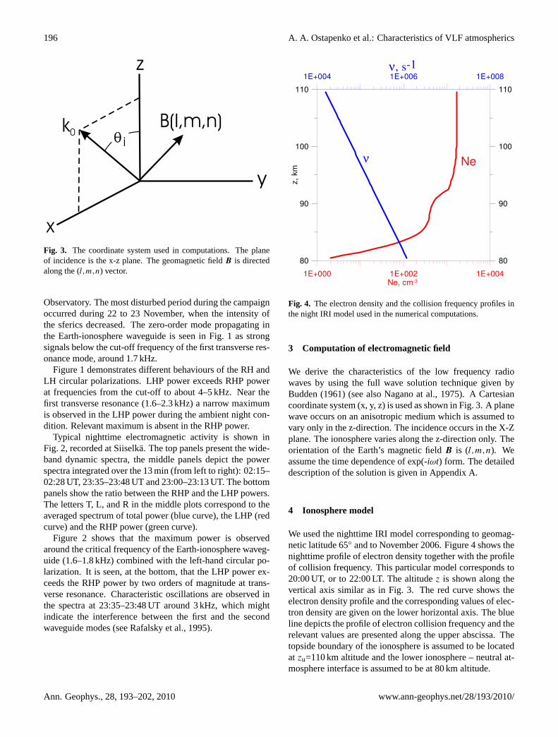
Fig. 4. The electron density and the collision frequency profiles inthe night IRI model used in the numerical computations.

3 Computation of electromagnetic field

We derive the characteristics of the low frequency radiowaves by using the full wave solution technique given byBudden (1961) (see also Nagano at al., 1975). A Cartesiancoordinate system (x, y, z) is used as shown in Fig. 3. A planewave occurs on an anisotropic medium which is assumed tovary only in the z-direction. The incidence occurs in the X-Zplane. The ionosphere varies along the z-direction only. Theorientation of the Earth’s magnetic fieldB is (l,m,n). Weassume the time dependence of exp(-iωt) form. The detaileddescription of the solution is given in Appendix A.

4 Ionosphere model

We used the nighttime IRI model corresponding to geomag-netic latitude 65◦ and to November 2006. Figure 4 shows thenighttime profile of electron density together with the profileof collision frequency. This particular model corresponds to20:00 UT, or to 22:00 LT. The altitudez is shown along thevertical axis similar as in Fig. 3. The red curve shows theelectron density profile and the corresponding values of elec-tron density are given on the lower horizontal axis. The blueline depicts the profile of electron collision frequency and therelevant values are presented along the upper abscissa. Thetopside boundary of the ionosphere is assumed to be locatedat zu=110 km altitude and the lower ionosphere – neutral at-mosphere interface is assumed to be at 80 km altitude.



Fig. 5. The penetration depth of the RHP waves (red curve) and ofthe LHP waves (blue line) at 1600 Hz frequency during the night-time.

5 Estimates of scale depth

During the night, we observe the resonance at a frequencyof about 1.6 kHz (see Fig. 2). Hence, the effective height ofthe ionosphere isλ2 =

c2·f

≈ 94 km. At this altitude, electron

density and collision frequency areNe=1.29×103 cm−3, andν=1.57×104 s−1, respectively. Relevant refractive indicesarenL = 0.05+6.3· i for the LHP andnR = 6.4+0.05· i forthe RHP wave in the magnetized plasma at 65◦ geomagneticlatitude. The LHP field amplitude varies as exp(ik0nLz) =

exp(−0.23·z). Hence, the scale height of this wave is equalto ζ=1/0.23=4.4 km.

We will regard below the scale height as “scale depth”.Figure 5 shows the scale depth of the 1.6 kHz wave as thefunction of altitude. The red curve corresponds to the RHPwave and the blue line shows LHP wave in the ambient nightconditions. It is clear that at 94 km, which correspond tothe first transverse resonance frequency, the scale depths are618 and 4.89 km for the RHP and LHP waves, respectively.The values depart by a factor of 130. This data indicatethat the LHP waves are effectively reflected from the iono-sphere, while the RHP waves have a large “scale depth”and are poorly reflected. In other words, the great “scaledepth” allows the RHP waves to escape into the magneto-sphere through the ionosphere.

6 Waveguide modes in the night ionosphere model

The roots of dispersion equation (A5) are the eigenvalues ofthe waveguide modes and their imaginary part determinesthe wave attenuation. The tangential electric field is equalto zero at the ground surface and the horizontal magnetic

field reaches the maximum here. The wave polarization atthe ground surface is defined as:

HR = Hx + i ·Hy, HL = Hx − i ·Hy, R= |HR|,

L = |HL |, ε =R−L

R+L(1)

We use the ellipticity parameterε, which is +1 for the cir-cular RHP wave and−1 for the circular LHP. In the generalcase, the sign ofε gives the sense (direction) of rotation ofthe field vector. Parameterε is positive for the RHP waves(i.e. the counter-clockwise rotation when the wave propa-gates along the Earth’s magnetic field) and it is negative forthe LHP waves.

Figure 6a shows attenuation coefficients for the first 5modes in the frequency range of 1–4 kHz computed fromEq. (A13). The modes are labelled in accordance to the right(R) or the left (L) polarizations; the numbers denote the modenumber. One may notice in Fig. 6a that the first-order and thesecond-order waveguide modes start to propagate from fre-quencies of 1.6 and 3.2 kHz. The “new-born” waves have ini-tially a large attenuation factor (at frequencies just above thecut-off). The attenuation rapidly decreases with frequencyand soon it reaches the level of the conventional losses in theEarth-ionosphere duct. It is also obvious that the attenua-tion factor of the LHP waves is smaller than that of the RHPwaves at all frequencies.

The real part of the longitudinal or the x-component of therefraction indexnx=kx /k0 is shown in Fig. 6b. It is relatedto the phase velocityVph by the formula Re (nx) = c/Vph.The zero-order modes of the waveguide L0 and R0 satisfythe relation:

n2= n2

x +n2z; nx = 1; nz = 0. (2)

The wave number at the transverse resonance satisfies thecondition:

kz =2π

λz

=π

h; kx =

√k2

0 −k2z ;

nx =kx

k0=

√1−

π2

(k0h)2. (3)

As it can be seen in Fig. 6b, the refraction index Re (nx) ≈ 1for the zero-order modes L0, R0, hence, these are the prop-agating modes. The zero-order mode TH0, which is also re-garded as the E0-wave, does not have the lower cut-off fre-quency. This mode supports the long distance ELF prop-agation at frequencies below the first transverse resonancefrequency (e.g. Kikuchi and Araki, 1979; Nickolaenko andHayakawa, 2002).

Frequency dependence of the L1 mode indicates its cap-ture by the waveguide at the frequency of the first transverseresonance. The refraction indexnx of this mode is equalto zero at the resonance frequency and it grows towards 1with the frequency increase. Electromagnetic energy of the



1 2 3 4

100

101

102

Atten

uatio

n, dB

/1000

km

f, kHz

L1

L0

R0

R1

L2

Fig. 6a. Attenuation factor of different modes for the night IRImodel of ionosphere.

1 2 3 40,0

0,5

1,0L0

R1

R0 L1

Re(n

x)

f, kHz

L2

Fig. 6b. X-component of refraction index for different modes.

first waveguide mode is “trapped” at the first transverse res-onance frequency. Indeed, according to the modal equationk2

= k2x +k2

z , we obtainkx = 0 in this case as 1− (kz)2= 0

at the particular resonance frequency off1 =c

2h. Physically,

the phase front of the trapped radio wave is horizontal, paral-lel to the boundaries. This wave is the standing wave. Owingto the particular frequency, nothing is left in the dispersionrelation for a non-zerokx component responsible for the hor-izontal propagation. Therefore, the wave is captured atf =f1and the Earth-ionosphere cavity acts as a planar Fabry-Perotresonator. All the sites at the ground surface will detect theradio wave with the zero mutual phase shift. A non-zerokx

component appears at higher frequencies and the first-orderwaveguide mode starts to propagate horizontally. The phasedelay appears with the frequency increase, which depends onthe length of the propagation path. This phase shift was ex-ploited for establishing the source-observer distance (Rafal-sky et al., 1995; Brundel et al., 2002). Finally, the wave frontturns into a vertical plane at the infinite frequency.

1 2 3 4-1

0

1 R0R1

L0 L1

ellip

ticity

,

f, kHz

L2

Fig. 6c. Polarization of different modes for the night IRI model ofionosphere.

Polarization ellipticityε is shown in Fig. 6c for differenteigenmodes. One can see that LHP wave has the circularpolarization at resonance frequencies, asε ≈ −1 here. TheLHP have the lowest attenuation rate above the resonancefrequency. This conclusion is confirmed by observations: theleft-hand polarized waves dominate at frequencies above thefirst transverse resonance.

The field amplitude reaches its maximum at the resonancefrequency in conventional resonance phenomena. One couldexpect a similar maximum in the amplitude spectrum oftransverse resonance, as it was observed in experiments withthe HF powerful transmitter of modulated amplitude (Stubbe,1982). However, computations predict a large attenuationfactor at the resonance frequency (Fig. 6a), so that radiowaves cannot propagate effectively in the Earth-ionosphereduct. Two questions arise. In what way does the narrowmaximum appear in the amplitude spectrum of the distantsferics? Does its position depend on the distance betweenthe source and observer?

7 Transverse resonance spectra excited by in-phase pla-nar current

We computed amplitude spectra excited by the in-phase pla-nar current placed below the nighttime ionosphere. The se-lection of the horizontal source current is justified by thefollowing reason. The transverse resonance is associatedwith radio waves trapped between the ground and the lowerionosphere (Lazebny et al., 1988; Rafalsky et al., 1995;Hayakawa et al., 1994, 1995; Nickolaenko and Hayakawa,2002). Such waves propagate vertically; hence, only hori-zontal current might be an effective source of the transverseresonance. In the case where the causative lightning dis-charge has a tilted channel, the horizontal projection of its



current serves as the field source for the transverse resonancesignals.

We use an infinite horizontal in-phase current sheet as thesource, which is positioned at the height of lightning dis-chargesz=7 km. The horizontal planar currentJ ext flowsin the Y-direction, so that only theBx component is present.The amplitude of the current is independent of frequency:J ext=const. Results of field computations are presented inFig. 7, where the source frequency is shown along the ab-scissa in kHz and the amplitude|Bx | is depicted along theordinate in arbitrary units. Our idealized source model al-lows obtaining the transverse resonance in the clearest fash-ion, demonstrated by Fig. 7.

The spectrum of Fig. 7 contains pronounced peaks cor-responding to two transverse resonance modes. The signalamplitude is increased by an order of magnitude owing tothe resonance. Amplitude of the second transverse resonancemode exceeds that of the basic mode. It is explained by thegrowing efficiency of horizontal source when the frequencyincreases.

Thus, in the vicinity of horizontal lightning discharge, onecan expect the amplitude maximum to be elevated over the“podium” by an order of magnitude. In the case of our ob-servations, the major sources were located at distances of afew thousands kilometres.

Figure 6 shows the wave attenuation factor exceeding20 dB per 1000 km at frequencies above the transverse res-onance. Such attenuation would compensate the excess ofthe resonance amplitude, provided that the distance from thesource to observer is 1000 km or more. Therefore, the exper-imental maximum seen in Fig. 1 could hardly be associatedwith the sub-ionospheric propagation: the field sources werea few thousand of kilometres away from the receiver. Thisis why we believe that regularly observed nocturnal spectralmaximum at 1.6–2.3 kHz frequency is connected with the lo-cal sources in the auroral zone.

We now consider the ratioRP of the quality factors per-tinent to the LHP and RHP oscillations. It is the in-verted ratio of the relevant attenuation rates:RP= QL/QR =

ImωR/ImωL . As seen in Fig. 6, the attenuation factor of theLHP waves is two orders of magnitude smaller than that ofthe RHP wave. This point explains why the LHP waves pre-vail in the observed resonance maxima, or in the “tail” oftweek atmospherics detected on the ground. The ionosphereis a rather good reflector for the LHP waves. Simultane-ously, the RHP waves easily penetrate into the ionosphereand escape from the Earth-ionosphere cavity into the mag-netosphere. The idea also explains the origin of “striped”spectral structures of transverse resonance detected on boardthe DEMETER and other satellites (Ferencz et al., 2007).

1 2 3 4

100

101

Bx, r

el. un

its

f, kHzFig. 7. Amplitude spectra of transverse resonance of the Earth-ionosphere cavity when excited by the infinite planar in-phase cur-rent placed at the 7 km altitude above the ground in the ambientnight conditions. The amplitude maxima are observed at transverseresonance frequencies of 1.6 and 3.2 kHz.

8 Discussion

The amplitude and polarization spectra of high latitude sfer-ics are often similar to those observed at the mid-latitudes(Yedemsky et al., 1992; Mikhaylova, 1988) or in the vicinityof the equator (Hayakawa et al., 1994, 1995).

The first-order mode radio wave has the LHP at all fre-quencies and it acquires the circular LHP at the resonance(or the cut-off) frequency of 1.7–1.8 kHz (Yedemsky et al.,1992; Hayakawa et al., 1994, 1995). Tweek amplitude spec-tra have the sharp maximum and a strong dispersion nearbythis frequency (Mikhaylova, 1988). Hayakawa et al. (1994,1995) used the full wave solution when modelling tweek po-larization in the Earth-ionosphere waveguide with a realisticelectron density profile. Our results confirm their conclusionthat the attenuation of the first mode LHP wave is much lowerthan that of the RHP waves. This is the reason why only theLHP waves are observed at frequencies just above the firstcut-off frequency of the Earth-ionosphere waveguide.

However, Hayakawa et al. (1994, 1995) do not explain thewell-pronounced amplitude maximum present in the spec-tra of the long distance tweeks: the peak is positioned atthe cut-off frequency (Mikhaylova, 1988). The emergenceof such a peak was addressed in works by Yamashita (1977)and Ryabov (1992, 1994). They have found that the atten-uation factor of the corresponding waveguide mode has anarrow minimum just above the Earth-ionosphere waveguidecut-off. Thus, the minimum of losses is observed as a sharpmaximum in the amplitude spectrum of tweeks.

Our computations are based on the full wave solution andthe obtained results deviate from those published by Ya-mashita (1977) and Ryabov (1992): we did not find any



minima in the wave attenuation rate around the transverseresonance (the waveguide cut-off) frequency. Therefore, themaximum in the amplitude spectrum of sferics at the criticalfrequency of the waveguide must be attributed to the trans-verse resonance of the Earth-ionosphere duct. Computationsperformed with the planar current source show a pure spec-trum of the transverse electromagnetic resonance, which cor-responds to radio waves captured between ground and theionosphere. Such waves are effectively excited by horizon-tal currents (e.g. Lasebny et al., 1988; Rafalsky et al., 1995;Nickolaenko and Hayakawa, 2002).

In reality, the remote field source has the finite horizon-tal dimension. Therefore, the radio propagation is alwayspresent in the experiment. Guided radio waves travel in aduct as a number of modes. Different modes interfere and theobserved amplitude spectrum becomes substantially modi-fied. A characteristic “mode beating” appears at every fre-quency of the transverse resonance (Rafalsky et al., 1995;Nickolaenko and Hayakawa, 2002). The clear resonance pat-tern might be observed only in the spectrograms of distantsferics.

The transverse resonance in its pure form might be ob-served only for a short distance between the source and ob-server. Such a situation was realised in the experiments ofionospheric HF heating (Stubbe at al., 1982). Sometimes thetransverse resonance is observed in the integrated daytimeELF-VLF power spectra, provided that a thunderstorm oc-curs close to the receiver (Lazebnyi et al., 1988; Belyaev etal., 1991).

9 Conclusion

We made a study of ELF-VLF sferics recorded in North-ern Finland. Sensitive receivers allowed the detection ofnatural radio waves and relevant polarization studies of thefield. Pronounced amplitude maximum was detected near thefirst transverse resonance frequency of the Earth-ionospherewaveguide (∼1.6 kHz) in night conditions. Received radiowaves had the circular LHP, which prevails at frequencies upto 4–5 kHz.

Experimental results are interpreted with the full wavesolution for the particular geometry of the nighttime iono-sphere. We found that the attenuation factor of the LHP waveis much smaller than that of the RHP wave, which allows theleakage of the RHP wave into the magnetosphere through theanisotropic ionosphere.

Transverse resonance spectra were computed for the fieldsource in the form of a planar infinite horizontal currentsheet. Analysis showed that transverse resonance becomesevident when the wave propagates only in the vertical direc-tion. This means that its convincing pattern might be ob-tained for the nearby sources.

The problem remains in the nearby field source at highlatitudes. To resolve this problem one has to treat the ex-

citation efficiency of remote horizontal lightning discharges(the wave propagating in the sub-ionospheric duct) and thisone of the signal arriving from the magnetosphere (the wavespropagating in plasma along the magnetic field lines).

Appendix A

The full wave solution

We derive the characteristics of the low frequency radiowaves by using the technique suggested by Budden (1961)(see also Nagano at al., 1975). A Cartesian coordinate sys-tem (x, y, z) is used as shown in Fig. 3. A plane wave isincident on an anisotropic medium from below at an angleθ

to the z-axis. The incidence occurs in the X-Z plane. Iono-sphere varies along the z-direction only. The orientation ofthe Earth’s magnetic field is (l, m, n). We assume the timedependence of the exp(−iωt) form. Electromagnetic fieldssatisfy the following Maxwell’s equations:

∇ ×H = −iωε0(I +M)E (A1)

∇ ×E = iωµ0B (A2)

whereε0, µ0 are the free space permittivity and permeabil-ity correspondingly,I denotes the unit matrix, andM is thesusceptibility matrix with the following elements:

Mxx = −X(U2− l2Y 2)/U(U2

−Y 2),

Mxy = −X(iUnY −nlY 2)/U(U2−Y 2),

Mxz = −X(−iUmY + lmY 2)/U(U2−Y 2),

Myx = X(−iUnY + lrnY 2)/U(U2−Y 2),

Myy = −X(U −m2Y 2)/U(U2−Y 2),

Myz = −X(iUIY −mnY 2)/U(U2−Y 2),

Mzx = −X(iUmY − lnY 2)/U(U2−Y 2),

Mzy = X(−iUnY )/U(U2−Y 2),

Mzx = −X(U −n2Y 2)/U(U2−Y 2),

Here, we apply the following symbols:U=1+iZ; Z=ν/ω;X=(ωp/ωH )2; ω2

p = e2N /mε0; ωH =eB/m; Y=ωH /ω; ωp isthe plasma circular frequency;ωH is the electron gyro fre-quency;m ande are the electron mass and its charge corre-spondingly;N is the electron density,v is the electron colli-sion frequency.

The ionosphere is the horizontally stratified medium andthe space-time dependence of each field component in the in-cident wave is proportional to exp[−iωt + ik0(nxx +nzz)],where k0 is the propagation constant of the free space,nx =sinθ , nz =cosθ . By eliminating theEz andHz compo-nents from Eqs. (1) and (2) and by applying the Snell’s law,we obtain the following equation (Budden, 1961):

de/dz = ik0Te, (A3)



wheree is the column matrix composed of the horizontalelectric and magnetic field components:

e=

Ex

Ey

Z0Hx

Z0Hy

, Z0 = (µ0/ε0)1/2 ,

andT is the 4×4 matrix

T =

−

nxMzx

1+Mzz

nxMzy

1+Mzz0 1−n2

x+Mzz

1+Mzz

0 0 −1 0MyzMzx

1+Mzz−Myx 1−n2

x +Myy −MyzMzy

1+Mzz0 nxMyz

1+Mzz

1+Mxx −MxzMzx

1+Mzz

MxzMzy

1+Mzz−Mxy 0 −

nxMxz

1+Mzz

.

If the medium is divided into a number of thin homogeneousslabs, formula (A3) becomes a differential equation with aconstant matrixT within each layer. Then, a particular solu-tion of Eq. (A3) corresponds to the factor exp(−ik0qz) com-bined with the complex wave amplitude. We obtain fromEq. (A3)

(T −qI)e= 0 (A4)

The condition of a nontrivial solution of Eq. (4) is:

Det(T −qI) = 0 (A5)

Relation (A5) gives the so-called Booker quadric equationfor q and the relevant eigen values determine the characteris-tic modes of upgoing and downgoing waves being each of theLHP and the RHP types. Equation (A5), within a homoge-neous layer, provides the eigenvalueql and Eq. (A4) allowsfor constructing the corresponding eigenvectors of the prob-lem.

Let us turn to the solution of the equation with a non-zeroright part:

dedz

− ik0Te= µ0J ext, (A6)

whereJ ext is the external source current. The general solu-tion of the fourth-order differential Eq. (A6) has the follow-ing form:

e=

i=4∑i=1

ci ·ei, (A7)

Here, the indexi denotes solutions (and eigenvalues) relevantto the LHP and RHP waves propagating upward (i=1, 2), orto the LHP and RHP waves propagating downward (i=3, 4).

Since the WKB approach is valid at the upper boundary ofthe ionosphere, the reflected waves are absent, and only thewaves travelling upward remain:

e=

i=2∑i=1

ci ·ei for z = zU (A8)

In a “straight marching” procedure, the partial solutionse1ande2 are constructed step by step downward starting at the

upper boundary and finishing at the ground surface. Thecoefficientsc1, c2 remain undefined. To establish them, aparticular solution of inhomogeneous Eq. (A6)enh must beadded to the general solution (A8)

e=

i=2∑i=1

ci ·ei +enh (A9)

Combination (A9) must satisfy the boundary conditions onthe perfectly conducting surface of the Earth and the un-known coefficientsc1, c2 are found.

The field discontinuities might be met. For example, a cur-rent sheetJ extv positioned in the ionosphere at the heightz0causes a discontinuity in the tangential magnetic induction:

{Bx} ≡(Bx2 −Bx1

)∣∣z=z0 = µ0J extv (A10)

while

Ex1

∣∣z=z0 = Ex2

∣∣z=z0 = Ey1

∣∣z=z0 = Ey1

∣∣z=z0 (A11)

or{c1Ex1+c2Ex2+Exnh= 0c1Ey1+c2Ey2+Eynh= 0

}(A12)

The solution of system (A12) is unique when the followingcondition is satisfied:∣∣∣∣∣∣Ex1 (z1) ; Ey1 (z1)

Ex1 (z1) ; Ey2 (z1)

∣∣∣∣∣∣ 6= 0

In the absence of source currentJ ext=0 the following disper-sion relation is obtained:∣∣∣∣∣∣Ex1 (z1) ; Ey1 (z1)

Ex1 (z1) ; Ey2 (z1)

∣∣∣∣∣∣ = 0 (A13)

It defines the complex eigenvalues: the phase velocity of ra-dio waves and the attenuation factor.

Acknowledgements.This work was supported by the RussianAcademy of Sciences (Program for Basic Research “Plasma Pro-cesses in the Solar System”) and EU LAPBIAT program (RITA-CT-2006-025969).

Topical Editor M. Pinnock thanks V. Pilipenko and anotheranonymous referee for their help in evaluating this paper.

References

Belyaev, P. P., Buzunkin, A. A., and Lisov, A. A.: Structure ofelectromagnetic noise spectra in waveguide Earth-ionosphere atfrequency (1–10) kHz., in The low frequency Earth-ionospherewaveguide, Publishing house “Gylym”, 90–96, 1991.

Brundell, J. B., Rodger, C. J., and Dowden, R. L.: Validation ofsingle-station lightning location technique, Radio Sci., 37(4), 12-1, 1059, doi:10.1029/2001RS002477, 2002.

Budden, K. G.: Radio waves in the ionosphere, Cambridge Univer-sity press., 1961.



Cummer, S. A.: Lightning and ionospheric remote sensing usingVLF/ELF radio atmospherics, PhD thesis, Dept. of Electrical En-gineering, Stanford University, Stanford, USA, 1997.

Felsen, L. B. and Marcuvitz, N.: Radiation and Scattering of Waves,Prentice-Hall, Englewood Cliffs, N.J., 888 p., 1973.

Ferencz, O. E., Ferencz, Cs., Steinbach, P., Lichtenberger, J.,Hamar, D., Parrot, M., Lefeuvre, F., and Berthelier, J.-J.: Theeffect of subionospheric propagation on whistlers recorded bythe DEMETER satellite – observation and modelling, Ann. Geo-phys., 25, 1103–1112, 2007,http://www.ann-geophys.net/25/1103/2007/.

Hayakawa, M., Ohta, K., and Baba, K.: Wave characteristics oftweek atmospherics deduced from the direction-finding measure-ment and theoretical interpretation, J. Geophys. Res., 99(05),10733–10743, 1994.

Hayakawa, M., Ohta, K., Shimakura, S., and Baba, K.: Recent find-ings on VLF/ELF sferics, J. Atmos. Terr. Phys., 57(5), 467–477,1995.

Kikuchi, T. and Araki, T.: Horizontal transmission of the polar elec-tric field to the equator, J. Atmos. Terr. Phys., 41, 927–936, 1979.

Lazebnyi, B. V., Nikolaenko, A. P., Rafal’skii, V. A., and Shvets, A.V.: Detection of transverse resonances of the earth-ionospherecavity in the mean spectrum of VLF atmospherics, Geomag-netism and Aeronomy, 28, 329–330, 1988.

Lysak, R. L.: Generilized model of the Ionospheric Alfven Res-onator, Geophys. Monogr. Ser., 80, 121–128, AGU, Washington,D.C., 1993.

Manninen, J.: Some aspects of ELF-VLF emissions in geophys-ical research, Publ. 98, Sodankyla Geophys. Obs., Sodankyla,Finland, available athttp://www.sgo.fi/Publications/SGO/thesis/ManninenJyrki.pdf), 2005.

Mikhailova, G. A. and Kapustina, O. V.: Finite frequency-timestructure of tweek atmospherics and VLF diagnostics of the pa-rameters of the nighttime lower ionosphere, Geomagnetizm iAeronomia, 28, 1015–1018, 1988.

Nagano, I., Mambo, M., and Hutatsuishi, G.: Numerical com-puttion of electromagnetic waves in an anisotropic multilayeredmedium, Radio Sci., 10(6), 611–617, 1975.

Nickolaenko, A. P. and Hayakawa, M.: Resonances in the Earth-ionosphere cavity, Kluwer Academic Publishers, Dordrecht-Boston-London, 380 p., 2002.

Rafalsky, V. A., Nickolaenko, A. P., Shvets, A. V., and Hayakawa,M.: Location of lightning discharges from a single station, J.Geophys. Res., 100(D10), 20829–20838, 1995.

Ryabov, B. S.: Tweek propagation peculiarities in the earth-ionosphere waveguide and low ionosphere parameters, Adv.Space Res., 12(6), 255–258, 1992.

Ryabov, B. S.: Tweek formation peculiarities, Geomagnetism andAeronomy, English Translation, 34(1), 60–66, 1994.

Schumann, W. O.: On the radiation free self-oscillations of a con-ducting sphere which is surrounded by an air layer and an iono-spheric shell, Zeitschrift und Naturfirschung, 7a, 149–154, 1952(in German).

Shvets, A. V. and Hayakawa, M.: Polarisation effects for tweekpropagation, J. Atmos. Solar-Ter. Phys., 60(4), 461–469, 1998.

Shvets, A. V.: On polarization properties of tweeks, Radio-Physicsand Electronics, 2(2), 101–106, 1997.

Shvets, A. V.: ELF-VLF remote sensing of the Earth – iono-sphere cavity, Doctor Degree Dissertastion in Phys-Math sci-ences, Kharkov, IRE, 308 pp., 2008.

Smirnov, V. S. and Ostapenko, A. A.: Transverse resonances ofEarth-ionosphere wave guide in auroral region Geomagnetismand Aeronomy, English Translation, 26(2), 253–257, 1986.

Stubbe, P., Kopka, H., and Rietveld, M. T.: ELF and VLF wave gen-eration by modulated HF heating of the current carrying lowerionosphere J. Atmos. Terr. Phys., 44(12), 1123–1135, 1982.

Yamashita, M.: Propagation of tweek atmospherics, J. Atmos. Terr.Phys., 40, 151–156, 1978.

Yedemsky, D. Y., Ryabov, B. S., Shchokotov, Yu. A., and Yarotsky,V. S.: Experimental investigation of the tweek lieid structure,Adv. Space. Res., 12(6), 251–254, 1992.


http://www.ann-geophys.net/25/1103/2007/

http://www.sgo.fi/Publications/SGO/thesis/ManninenJyrki.pdf

http://www.sgo.fi/Publications/SGO/thesis/ManninenJyrki.pdf

characteristics of vlf atmospherics near the resonance

Documents