characteristics of i/o traffic in personal computer and
TRANSCRIPT

Characteristics of I/O Traffic inPersonal Computer and Server Workloads
Windsor W. Hsu†?
Alan Jay Smith?
†Storage Systems DepartmentAlmaden Research Center
IBM Research DivisionSan Jose, CA 95120
?Computer Science DivisionEECS Department
University of CaliforniaBerkeley, CA 94720
{windsorh,smith}@cs.berkeley.edu
Report No. UCB/CSD-02-1179
April 2002
Computer Science Division (EECS)University of CaliforniaBerkeley, California 94720


Characteristics of I/O Traffic inPersonal Computer and Server Workloads
Windsor W. Hsu†?
Alan Jay Smith?
†Storage Systems DepartmentAlmaden Research CenterIBM Research Division
San Jose, CA [email protected]
?Computer Science DivisionEECS Department
University of CaliforniaBerkeley, CA 94720
{windsorh,smith}@cs.berkeley.edu
Abstract
Understanding the characteristics of physical I/O trafficis increasingly important as the performance gap betweenprocessor and disk-based storage continues to widen. More-over, recent advances in technology, coupled with marketdemands, have led to several new and exciting developmentsin storage, including network storage, storage utilities, andintelligent self-optimizing storage. In this paper, we em-pirically examine the I/O traffic of a wide range of real PCand server workloads with the intent of understanding howwell they will respond to these new storage developments.As part of our analysis, we compare our results with his-torical data and reexamine rules of thumb that have beenwidely used for designing computer systems. Our resultsshow that there is a strong need to focus on improving I/Operformance. We find that the I/O traffic is bursty and ap-pears to exhibit self-similar characteristics. In addition, ouranalysis indicates that there is little cross-correlation in traf-fic volume among the server workloads, which suggests thataggregating these workloads will likely help to smooth outthe traffic and enable more efficient utilization of resources.We also discover that there is a lot of potential for harnessing
Funding for this research has been provided by the State ofCalifornia under the MICRO program, and by AT&T Laboratories,Cisco Corporation, Fujitsu Microelectronics, IBM, Intel Corpora-tion, Maxtor Corporation, Microsoft Corporation, Sun Microsys-tems, Toshiba Corporation and Veritas Software Corporation.
“free” system resources for purposes such as automatic opti-mization of disk block layout. In general, the characteristicsof the I/O traffic are relatively insensitive to the amount ofcaching upstream and our qualitative results apply when theupstream cache is increased in size.
1 Introduction
Processor performance has been increasing at the rateof 60% per year while disk access time, being limited bymechanical delays, has been improving by less than 10%per year [16, 39]. Compounding this widening performancegap between processor and disk storage is the fact thatdisk capacity has been improving by more than 60% peryear [16, 39] so that each disk is responsible for the stor-age and retrieval of rapidly increasing amounts of data. Theoverall result of these technology trends, which show nosigns of easing, is that computer systems are increasinglybottlenecked by disk-based storage systems. The key step inovercoming this bottleneck is to understand how storage isactually used so that new optimization techniques and algo-rithms can be designed.
In addition, new paradigms and developments have re-cently emerged in the storage industry, and determining thereal effect of these requires a focused examination of theI/O characteristics of real workloads. First, storage is in-creasingly placed on some form of general network so that
1

it can be shared and accessed directly by several comput-ers at the same time [48] (e.g.,Network Attached Storage(NAS) for file storage and Storage Area Networks (SANs)for block storage). The performance of such network stor-age hinges on knowing the I/O traffic patterns and opti-mizing the network for such patterns. Second, consolidat-ing the storage now distributed throughout an organization,for instance to storage utilities or Storage Service Providers(SSPs), is expected to become increasingly popular [28].Whether such an approach leads to more efficient poolingof resources among different groups of users depends on thecharacteristics of their workloads, specifically on whetherthe workloads are independent. In practice, we will needrules of thumb that describe the storage and performance re-quirements of each group, as well as realistic traffic models.Third, the rapid growth in available processing power in thestorage system [14, 19] makes it possible to build intelligentstorage systems that can dynamically optimize themselvesfor the workload [22]. The design of these systems requiresa good understanding of how real workloads behave.
In this research, therefore, we empirically examine thestorage usage characteristics of real users and servers fromthe perspective of evaluating these new storage opportuni-ties. A total of 18 traces gathered from a wide range of envi-ronments are examined. We focus in this paper on analyzingthe I/O traffic, specifically, (1) the I/O intensity of the work-loads and the overall significance of I/O in the workloads,(2) how the I/O load varies over time and how it will be-have when aggregated, and (3) the interaction of reads andwrites and how it affects performance. We compare our re-sults with historical data to note any trends and to revalidaterules of thumb that are useful for systems design and sizing.To make our results more broadly applicable, we also studythe effect of increased upstream caching on our analysis. In acompanion paper, we examine how these real workloads areaffected by disk improvements and I/O optimizations such ascaching and prefetching [18]. The insights gained from thisresearch are instrumental to the block reorganization tech-nique outlined in [22].
The rest of this paper is organized as follows. Section 2contains a brief overview of previous work in characterizingI/O behavior. Section 3 discusses our methodology and de-scribes the traces that we use. In Sections 4-7, we analyzethe I/O traffic of our various workloads in detail. Concludingremarks appear in Section 8. Because of the huge amount ofdata that is involved in this study, we present only a charac-teristic cross-section in the main text. More detailed graphsand data are presented in Appendix A. Some of the moreinvolved mathematical material appears in Appendix B.
2 Related Work
I/O behavior at the file system level has been character-ized in some detail (e.g., [4, 8, 36, 42, 51]). There have
also been several studies of the logical I/O characteristicsof large database and scientific systems; see [20, 21] for abrief bibliography. These studies provide valuable insightsfor designing the file system and the database data managerbut they are not very useful for understanding what happensat the physical or storage level. Because of the file systemcache or the database buffer pool, most of the logical ref-erences never reach the physical storage. In addition, thelogical I/O behavior does not reflect the effects of file allo-cation and mapping. Furthermore, many of these studies donot account for system generated traffic such as paging andmetadata access, which can account for a significant fractionof the total I/O [42, 45].
Compared to the analysis of I/O behavior at the logicallevel, physical I/O characterization has received much lessattention in the research community. Part of the reason isthat storage level characteristics are sensitive to the file sys-tem or buffer pool design and implementation so that theresults of any analysis are less broadly applicable. But thisis precisely the reason to analyze the physical I/O character-istics of different systems. Traces collected from large IBMmainframe installations [49] and production VAX/VMS sys-tems [7, 24] have been used to study design issues in diskcaches. There has also been some analysis of the physicalI/O characteristics of Unix systems [45] and Novel NetWarefile servers [17] in academic/research environments. Eventhough personal computers (PCs) running various flavors ofMS Windows are now an integral part of many office ac-tivities, there has, to the best of our knowledge, been nopublished systematic analysis of how storage is used in suchsystems.
3 Methodology
Trace data can generally be gathered at different levels inthe system depending on the purpose of collecting the data.For instance, to evaluate cache policies for the file systembuffer, I/O references have to be recorded at the logical level,before they are filtered by the file system buffer. In general,collecting trace data at the logical level reduces dependen-cies on the system being traced and allows the trace to beused in a wider variety of studies, including simulations ofsystems somewhat different from the original system. Forinstance, to study physical storage systems, we could filter alogical trace through models of the file system layer to ob-tain a trace of the physical I/Os. A commonly used methodfor obtaining such a logical trace is to insert a filter driverthat intercepts all requests to an existing file system deviceand records information about the requests before passingthem on to the real file system device.
However, this approach does not account for I/Os thatbypass the file system interface (e.g.,raw I/O, virtual mem-ory paging and memory-mapped I/O). Recent results [42]show that 15% of reads and nearly 30% of writes in Win-
2

dows NT workloads can be attributed to paging by runningprograms. In addition, 85% of processes now memory-mapfiles compared with 36% that read files and 22% that writethem. From a practical perspective, the approach of startingwith a logical trace to evaluate physical storage systems re-quires that a lot of data be collected, which adds disturbanceto the systems being traced, and then painstakingly filteredaway by simulating not only the buffer cache and prefetcherbut also how the data is laid out and how the metadata isreferenced. For today’s well-tuned systems, each of thesecomponents is complicated and the details of their operationare seldom publicly available. For instance, the file systembuffer on many systems (e.g., Windows NT) is integratedwith the memory manager and dynamically sized based onperceived workload characteristics. Therefore the net resultof taking a logical trace and filtering it through models of thefile system components is not likely to reflect the workloadseen by any real storage system. Since file systems todayare relatively stable and rarely undergo radical changes, webelieve that in general, for the purpose of studying physicalstorage systems, analyzing traces collected at the physicallevel is more practical and realistic. This is the method weuse in this paper.
In order to make our characterization more useful forsubsequent mathematical analyses and modeling by oth-ers, we have fitted our data to various functional formsthrough non-linear regression, which we solved by usingthe Levenberg-Marquardt method [40]. When appropriate,we also fitted standard probability distributions to our databy using the method of maximum likelihood to obtain pa-rameter estimates and then optimizing these estimates by theLevenberg-Marquardt algorithm [40].
3.1 Trace Collection
The traces analyzed in this study were collected fromthree different platforms, namely Windows NT, IBM AIXand HP-UX. A different trace facility was used on eachplatform. The Windows NT traces were collected by usingVTrace [29], a software tracing tool for Intel x86 PCs run-ning Windows NT and Windows 2000. VTrace was primar-ily developed to collect data for energy management studiesfor portable computers. In this study, we are mainly inter-ested in the disk activities, which are collected by VTracethrough the use of device filters. VTrace takes daily snap-shots of the NTFS file system metadata. In addition, it col-lects data on the file system as well as process and threadactivities. We have verified the disk activity collected byVTrace by comparing it with the raw SCSI traffic obtainedby a SCSI analyzer. Details of VTrace and the special tech-niques used to collect the relevant data with minimal intru-sion can be found in [29].
After VTrace is installed on a system, each disk requestgenerates a trace record consisting of the time (based on the
Intel Pentium cycle counter), sequence number, file objectpointer, disk and partition numbers, start address, transfersize, and flags describing the request (e.g.,read, write, syn-chronous). After the disk request has been serviced, a com-pletion record is written. In a post processing step, we matchup the sequence number recorded in the request and comple-tion records to obtain the service times. To better understandthe I/O behavior of the system, it is useful to be able to as-sociate each disk request with the name of the correspond-ing file and process. In most cases, we are able to matchup the file object pointer with a file open record to obtainthe filename. When the match fails, we try to determine thefilename by looking up the block address in a reverse allo-cation map that is constructed from the periodic metadatasnapshots.
Because VTrace is designed to collect data for energymanagement studies, it also gathers data about process andthread creations and deletions as well as thread switches. Byusing the thread create and thread switch trace records, weare able to match up I/O requests with the names of the re-questing processes. In addition, the thread switch recordsenable us to determine the overall significance of I/O in theseworkloads. We will look at this in Section 4.1.
To keep the amount of data collected manageable, pro-cess and thread trace records are gathered only for a span ofone and a half hours every three and a half hours. In addi-tion, all trace collection is turned off ten minutes after thecessation of user mouse and keyboard activity. Newer ver-sions of VTrace collect some trace data all the time but inorder to have a consistent set of data, we have processed thetraces used in this study to delete trace records that occur af-ter ten minutes of user idle time. In other words, we use onlythe trace records that occur from the first user activity afteran idle period to the last user activity before an idle period;we assume that there is no activity in the system during theperiods when the user is idle. We believe that this is a rea-sonable approximation in the PC environment, although it ispossible that we are ignoring some level of activity due toperiodic system tasks such as daemons. This latter type ofactivity should have a negligible effect on the I/O load, al-though it might be important for other types of studies, suchas power usage.
Both the IBM AIX and HP-UX traces were collected us-ing kernel-level trace facilities built into the operating sys-tems. These trace facilities are completely transparent to theuser and adds no noticeable processor load. Among the in-formation collected for each physical I/O are: timing infor-mation, disk and partition numbers, start address, transfersize and flags describing the request. More details about theIBM AIX trace facility can be found in [23]. The HP-UXtrace facility is described in [45].
3

System Configuration Trace CharacteristicsDesign-
ation User TypeSystem Memory
(MB) File Systems StorageUsedi (GB) # Disks Duration Footprintii
(GB)Traffic(GB)
Requests(106)
P1 Engineer 333MHz P6 64 1GB FATi 5GB NTFSi 6 1 45 days (7/26/99 - 9/8/99) 0.945 17.1 1.88
P2 Engineer 200MHz P6 64 1.2, 2.4, 1.2GB FAT 4.8 2 39 days (7/26/99 - 9/2/99) 0.509 9.45 1.15
P3 Engineer 450MHz P6 128 4, 2GB NTFS 6 1 45 days (7/26/99 - 9/8/99) 0.708 5.01 0.679
P4 Engineer 450MHz P6 128 3, 3GB NTFS 6 1 29 days (7/27/99 - 8/24/99) 4.72 26.6 2.56
P5 Engineer 450MHz P6 128 3.9, 2.1GB NTFS 6 1 45 days (7/26/99 - 9/8/99) 2.66 31.5 4.04
P6 Manager 166MHz P6 128 3, 2GB NTFS 5 2 45 days (7/23/99 - 9/5/99) 0.513 2.43 0.324
P7 Engineer 266MHz P6 192 4GB NTFS 4 1 45 days (7/26/99 - 9/8/99) 1.84 20.1 2.27
P8 Secretary 300MHz P5 64 1, 3GB NTFS 4 1 45 days (7/27/99 - 9/9/99) 0.519 9.52 1.15
P9 Engineer 166MHz P5 80 1.5, 1.5GB NTFS 3 2 32 days (7/23/99 - 8/23/99) 0.848 9.93 1.42
P10 CTO 266MHz P6 96 4.2GB NTFS 4.2 1 45 days (1/20/00 – 3/4/00) 2.58 16.3 1.75
P11 Director 350MHz P6 64 2, 2GB NTFS 4 1 45 days (8/25/99 – 10/8/99) 0.73 11.4 1.58
P12 Director 400MHz P6 128 2, 4GB NTFS 6 1 45 days (9/10/99 – 10/24/99) 1.36 6.2 0.514
P13 Grad. Student 200MHz P6 128 1, 1, 2GB NTFS 4 2 45 days (10/22/99 – 12/5/99) 0.442 6.62 1.13
P14 Grad. Student 450MHz P6 128 2, 2, 2, 2GB NTFS 8 3 45 days (8/30/99 – 10/13/99) 3.92 22.3 2.9
P-Avg. - 318MHz 109 - 5.07 1.43 41.2 days 1.59 13.9 1.67
(a) Personal Systems.
System Configuration Trace CharacteristicsDesign-
ationPrimaryFunction System Memory
(MB) File Systems StorageUsedi (GB)
#Disks Duration Footprintii
(GB)Traffic(GB)
Requests(106)
FS1 File Server(NFSiii)
HP 9000/720(50MHz)
32 3 BSDiii FFSiii (3 GB) 3 3 45 days (4/25/92 - 6/8/92) 1.39 63 9.78
FS2iv File Server(AFSiii)
IBM RS/6000 - 23 AIXiii JFSiii (99.1GB) 99.1 17 8am – 6pm (11/6/2000) - 1.70 -
TS1 Time-SharingSystem
HP 9000/877(64MHz)
96 12 BSD FFS (10.4GB) 10.4 8 45 days (4/18/92 - 6/1/92) 4.75 123 20
DS1Database
Server(ERPiii)
IBM RS/6000R30 SMPiii
(4X 75MHz)768
8 AIX JFS (9GB), 3 paging(1.4GB), 30 raw database
partitions (42GB)52.4 13 7 days (8/13/96 – 8/19/96) 6.52 37.7 6.64
S-Avg.v - - 299 - 18.5 8 32.3 days 4.22 74.6 12.1
i Sum of all the file systems and allocated volumes.ii Amount of data referenced at least once (using block size of 512 bytes)iii AFS – Andrew Filesystem, AIX – Advanced Interactive Executive (IBM’s flavor of UNIX), BSD – Berkeley System Development Unix, ERP – Enterprise Resource Planning, FFS – FastFilesystem, JFS – Journal Filesystem, NFS – Network Filesystem, NTFS – NT Filesystem, SMP – Symmetric Multiprocessoriv Only per second I/O statistics were collected.v Excluding FS2.
(b) Servers.
Table 1: Trace Description.
4

0
1
2
3
4
5
6
7
8
0 0.5 1 1.5 2 2.5 3# Requests (Millions)
Ref
eren
ceFo
otpr
int(
GB)
P1 P2 P3 P4P5 P6 P7 P8P9 P10 P11 P12P13 P14 P-Avg. FS1TS1 DS1
Figure 1: Footprint Vs. Number of References.
3.2 Trace Description
In this study, we use traces collected from both serverand personal computer (PC) systems. Table 1 summarizesthe characteristics of the traces. Thefootprint of a trace isdefined as the amount of data referenced at least once in thetrace. Figure 1 plots the trace footprint as a function of thenumber of references, which is a measure of the trace length.Similar plots for the read footprint and the write footprint arein Figure A-1 in Appendix A.
The PC traces are denoted as P1, P2, ..., P14. The term“P-Avg.” represents the arithmetic mean of the results for thePC traces. These traces were collected over a period rang-ing from about a month to well over nine months on PCsrunning Windows NT. In this study, we utilize only the first45 days of the traces. In addition to engineers and graduatestudents, the users of these systems also include a secretaryand several people in senior managerial positions. By hav-ing users ranging from managers and a secretary to hard coreengineers in our sample, we believe that our traces are illus-trative of the PC workloads in many offices, especially thoseinvolved in research and development. Note, however, thatthe traces should not be taken as typical or representative ofany other system. Despite this disclaimer, the fact that manyof our results correspond to those obtained previously, albeitin somewhat different environments, suggest that our find-ings are generalizable to a large extent.
The servers examined include two file servers, a time-sharing system and a database server. Throughout this pa-per, we use the term “S-Avg.” to denote the arithmetic meanof the results for the server workloads. The first file serverworkload (FS1) was taken off a file server for nine clientsat the University of California, Berkeley. This system was
primarily used for compilation and editing. It is referred toas “Snake” in [45]. The second file server workload (FS2)was taken off an Andrew File System (AFS) server at one ofthe major development sites of a leading computer storagevendor. The system was the primary server used to supportthe development effort. For this system, only per-second ag-gregate statistics of the I/O traffic were gathered; addressesfor individual I/Os were not collected. The trace denotedTS1 was gathered on a time-sharing system at an indus-trial research laboratory. It was mainly used for news, mail,text editing, simulation and compilation. It is referred to as“cello” in [45]. The database server trace (DS1) was col-lected at one of the largest health insurers nationwide. Thesystem traced was running an Enterprise Resource Planning(ERP) application on top of a commercial database.
Our traces capture the actual workloads that are pre-sented to the storage system and are therefore likely to besensitive to the amount of filtering by the file system cacheand/or the database buffer pool. However, we believe thatchanging the amount of caching upstream will only affectour characterization quantitatively and that the qualitativeresults still apply. To show that our characterization is rel-atively insensitive to the amount of caching upstream, wefiltered our traces through a Least-Recently-Used (LRU)write-back cache to obtain another set of traces on which torun our analysis. We denote these filtered traces by addingan “f” to the original designation. For instance, the trace ob-tained by filtering P1 is denoted as P1f. We also denote theaverage result for the filtered PC workloads as “Pf-Avg” andthat for the filtered server workloads as “Sf-Avg”. Follow-ing the design of most file systems, we allow a dirty blockto remain in the cache for up to 30 seconds. When a blockis written back, we write out, in the same operation, all thedirty blocks that are physically contiguous up to a maximumof 512 blocks. The size of the cache is chosen to be the sizeof the entire main memory in the original systems (Table 1).
In Table 2, we present the faction of I/O activity that isfiltered out by such a cache. On average, over 50% of theI/O requests are removed by the cache, which shows thatthe amount of caching has been significantly increased overwhat was in the original traced systems. Observe further thatthe traffic volume is reduced less significantly than the num-ber of operations. This is because the smaller requests tendto have a higher chance of hitting in the cache. Furthermore,by delaying the writes, we are able to consolidate them intolarger sequential writes. In Table 3 and Figure 2, we presentthe request size distribution for both the original and the fil-tered traces. Although the average request size of writes isincreased, the request size distributions of the filtered tracestrack those of the original traces remarkably well. That thefiltered traces maintain the qualitative behavior of the origi-nal traces is a result that we will see repeated in the rest ofthe paper.
5

0
20
40
60
80
100
1 10 100Request Size (# 512-byte Blocks)
Cum
ulat
ive
%of
Req
uest
s
P-Avg.
Pf-Avg.
FS1
TS1
DS1
S-Avg.
Sf-Avg.
Read Requests
0
20
40
60
80
100
1 10 100Request Size (# 512-byte Blocks)
Cum
ulat
ive
%of
Req
uest
s
P-Avg.
Pf-Avg.
FS1
TS1
DS1
S-Avg.
Sf-Avg.
Write Requests
Figure 2: Distribution of Request Size.
Number of MBs Number of Requests
Read Write Overall Read Write Overall
P1 0.575 0.176 0.441 0.618 0.575 0.605
P2 0.503 0.173 0.385 0.547 0.495 0.525
P3 0.583 0.163 0.291 0.632 0.498 0.537
P4 0.301 0.175 0.219 0.358 0.630 0.527
P5 0.369 0.232 0.275 0.438 0.620 0.574
P6 0.831 0.190 0.436 0.821 0.548 0.617
P7 0.546 0.143 0.246 0.551 0.548 0.549
P8 0.592 0.239 0.426 0.629 0.657 0.642
P9 0.484 0.146 0.317 0.488 0.471 0.479
P10 0.216 0.162 0.192 0.316 0.537 0.436
P11 0.515 0.245 0.409 0.520 0.641 0.577
P12 0.416 0.179 0.290 0.450 0.721 0.601
P13 0.557 0.257 0.391 0.585 0.615 0.603
P14 0.356 0.221 0.282 0.415 0.683 0.596
P-Avg. 0.489 0.193 0.329 0.526 0.589 0.562
FS1 0.594 0.573 0.582 0.570 0.681 0.633
TS1 0.583 0.394 0.474 0.546 0.454 0.495
DS1 0.057 0.203 0.122 0.133 0.702 0.488
S-Avg. 0.412 0.390 0.393 0.416 0.612 0.539
Table 2: Fraction of I/O Activity that is Filtered.
All Requests Read Requests Write Requests
Avg. Std.Dev. Min. Max. Avg. Std.
Dev. Min. Max. Avg. Std.Dev. Min. Max.
P1 19.1 26.6 1 128 17.7 22 1 128 22.4 35.4 1 128
P2 17.2 27.4 1 1538 19.1 24.4 1 128 14.6 30.9 1 1538
P3 15.5 24.8 1 128 15.5 19.4 1 128 15.5 26.8 1 128
P4 21.7 33.8 1 128 20.4 30.3 1 128 22.5 35.8 1 128
P5 16.3 25 1 298 20.8 28.3 1 129 14.8 23.6 1 298
P6 15.7 23.7 1 128 23.1 25.5 1 128 14.7 23.2 1 128
P7 18.5 30.3 1 128 19.1 23.9 1 128 18.4 31.9 1 128
P8 17.4 25.8 1 128 16.8 20.9 1 128 18.2 30.9 1 128
P9 14.7 21.1 1 128 15.4 20.2 1 128 13.9 21.8 1 128
P10 19.6 30.7 1 128 23.7 32.8 1 128 15.7 28 1 128
P11 15.2 23.1 1 128 19.4 24.7 1 128 11.7 21.1 1 128
P12 25.3 58.6 1 512 27.5 54.6 1 512 23.6 61.4 1 512
P13 12.3 18.2 1 180 14.5 18.8 1 128 11 17.7 1 180
P14 16.1 28.1 1 1539 20.6 31.2 1 128 14 26.2 1 1539
P-Avg. 17.5 28.4 1 373 19.5 26.9 1 156 16.5 29.6 1 373
Pf-Avg. 27.4 64.3 1 512 21.3 29.3 1 155 34.1 84.2 1 512
FS1 13.5 5.08 2 512 12.5 5.47 2 64 14.2 4.65 2 512
TS1 12.9 7.77 2 512 12.4 6.52 2 224 13.3 8.62 2 512
DS1 11.9 21.9 1 512 17.4 27.1 1 512 8.55 17.3 1 256
S-Avg. 12.8 11.6 1.67 512 14.1 13.0 1.67 267 12.0 10.2 1.67 427
Sf-Avg. 16.4 29.8 1.67 512 14.0 13.5 1.67 222 18.9 41.0 1.67 512
Table 3: Request Size (Number of 512-Byte Blocks).
6

0
5
10
15
20
25
30
35
40
P1 P2 P3 P4 P5 P6 P7 P8 P9 P10
P11
P12
P13
P14
P-Av
g.
Workload
Perc
ento
fTim
e
Both Busy
Disk Busy
Proc. Busy
0
10
20
30
40
50
60
70
80
90
100
P1 P2 P3 P4 P5 P6 P7 P8 P9 P10
P11
P12
P13
P14
P-Av
g.
Workload
Perc
ento
fBus
yTi
me
Both Busy
Disk Busy
Proc. Busy
Figure 3: Disk and Processor Busy Time.
4 Intensity of I/O
We begin our characterization by focusing on the I/O in-tensity of the various workloads. This is akin to understand-ing the size of a problem so that we can better approach it.The questions we seek to address in this section include howsignificant is the I/O component in the overall workload,how many I/Os are generated, and how fast do the requestsarrive.
4.1 Overall Significance of I/O
In Figure 3, we present the percent of time the disk andprocessor are busy for the PC workloads. Similar results forthe server workloads would be interesting but unfortunately,this analysis relies on information that is available only in thePC traces. The processor busy time is obtained by lookingat the thread switch records to determine when the processoris not in the idle loop. The disk busy time is taken to be theduration during which one or more of the disks in the systemare servicing requests. Recall that we only have trace datafor the periods during which user input activity occurs atleast once every ten minutes. In other words, we consideronly the periods during which the user is actively interactingwith the system.
From the figure, the processor is, on average, busy foronly about 10% of the time while the disk is busy for onlyabout 2.5% of the time. This low level of busy time is mis-leading, however, because the user is interested in responsetime; CPU idle generally represents user think time, andwould occur in any case in a single user environment. Thuswe cannot conclude that the processor and I/O system are”fast enough”. What the results do suggest is thatthere is alot of idle time for performing background tasks, even with-
out having to deliberately leave the computer on when theuser is away. In other words, significant resources are avail-able without requiring additional power consumption. Thechallenge is to harness these idle resources without affect-ing the foreground work. If this can be done unobtrusively,it will pave the way for sharing idle resources in collabo-rative computing, a paradigm commonly referred to as peer-to-peer (P2P) computing [32]. In addition, the idle resourcescan be used to optimize the system so that it will performbetter in future for the foreground task (e.g.,[22]). We willcharacterize the disk idle periods in detail in Section 5.3.
I/O is known to be a major component of server work-loads (e.g.,[43]). But if processors continue to increase inperformance according to Moore’s Law (60% per year) asmany believe they will,I/O may also become the dominantcomponent of personal computer workloads in the next fewyears. More memory will of course be available in the fu-ture for caching but the PC systems in our study are alreadywell-endowed with memory. A common way of hiding I/Olatency is to overlap it with some computation either throughmultiprogramming or by performing I/O asynchronously.From Figure 3, this technique appears to be relatively in-effective for the PC workloads sinceonly a small fraction(20% on average) of the disk busy time is overlapped withcomputation. In Figure 4, we compare the processor busytime during the disk idle intervals with that during the diskbusy intervals. A disk idle interval refers to the time inter-val during which all the disks are idle. A disk busy intervalis simply the period of time between two consecutive diskidle intervals. Reflecting the low average processor utiliza-tion of the workloads, the processor is busy less than 20%of the time for the long intervals (> 0.1s), regardless ofwhether any of the disks are busy. During the short inter-vals (< 0.1s), the processor is busy almost all the time when
7

0
10
20
30
40
50
60
70
80
90
100
0.0001 0.001 0.01 0.1 1 10Interval Size (s)
Proc
esso
rBus
yTi
me
(%In
terv
al)
Disk Busy Intervals
Disk Idle Intervals
Figure 4: Processor Busy Time during Disk Busy/Idle Inter-vals. Bars indicate standard deviation (To reduce clutter, weshow only the deviation in one direction).
Request Issued
Request CompletedR1 R2 R3 R4 R5
R1R0 R3Time
X1
X2
X3
X4
X5
Figure 5: Intervals between Issuance of I/O Requests andMost Recent Request Completion.
all the disks are idle but the processor utilization drops toless than 50% when one or more of the disks are busy. Suchresults imply thatlittle processing can be overlapped withI/O so that I/O response time is important for these kinds ofworkloads.
That only a small amount of processing is overlappedwith I/O suggests that there is effectively little multiprocess-ing in the PC workloads. Such predominantly single-processworkloads can be modeled by assuming that after complet-ing an I/O, the system has to do some processing and theuser, some “thinking”, before the next set of I/Os can be is-sued. For instance, in the timeline in Figure 5, after requestR0 is completed, there are delays during which the system isprocessing and the user is thinking before requestsR1, R2andR3 are issued. BecauseR1, R2 andR3 are issued afterR0 has been completed, we consider them to be dependenton R0. Similarly, R4 and R5 are deemed to be dependenton R1. Presumably, if R0 is completed earlier, R1, R2 andR3 will be dragged forward and issued earlier. If this in turncauses R1 to be finished earlier, R4 and R5 will be similarlymoved forward in time. In Figure 6, we plot the percent oftime the processor is busy during the interval between whenan I/O request is issued and the most recent completion of
0
10
20
30
40
50
60
70
80
90
100
0.0001 0.001 0.01 0.1 1 10 100Interval Between I/O Issue and Last I/O Completion (s)
Proc
esso
r/Ker
nelB
usy
Tim
e(%
Inte
rval
)
Proc. Busy
Kernel Busy
f(x)=1/(0.0857x+0.0105)
r2 = 0.985
f(x)=1/(28.7x+0.060)
r2=0.956
Figure 6: Processor/Kernel Busy Time during Intervals be-tween Issuance of I/Os and Most Recent Request Comple-tion. Bars indicate standard deviation (To reduce clutter, weshow only the deviation in one direction).
an I/O request (thex′s in Figure 5). We are interested inthe processor busy time during such intervals to model whathappens when the processing time is reduced through fasterprocessors.
From Figure 6, we find that for the PC workloads, theprocessor utilization during the intervals between I/O is-suance and the last I/O completion is related to the lengthof the interval by a reciprocal function of the formf(x) =1/(ax + b) wherea = 0.0857 andb = 0.0105. The recipro-cal function suggests that there is a fixed amount of process-ing per I/O. To model a processor that isn times faster thanwas in the traced system, we would scale only the systemprocessing time byn, leaving the user think time unchanged.Specifically, we would replace an interval of lengthx by oneof x[1− f(x) + f(x)/n]. We believe that for the PC work-loads, this is considerably more realistic than simply scalingthe inter-arrival time between I/O requests byn, as is com-monly done. In Figure 6, we also plot the percent of timethat the kernel is busy during the intervals between when anI/O request is issued and the previous I/O completion. Weconsider the kernel to be busy if the kernel process (processID = 2 in Windows NT) is allocated the CPU. As shown inthe figure, the kernel busy time is also related to the lengthof the interval by a reciprocal function, as we would expectwhen there is some fixed kernel cost per I/O.
This workload model is based on the assumption thatI/Os tend to be synchronous, meaning that the system hasto wait for I/Os to be completed before it can continue withits processing. As shown in Table 4, this is a reasonableassumption, especially for the PC workloads where, despite
8
Read Write Overall
P1 0.974 0.667 0.887
P2 0.970 0.627 0.825
P3 0.931 0.701 0.770
P4 0.829 0.731 0.768
P5 0.927 0.776 0.814
P6 0.967 0.849 0.864
P7 0.878 0.723 0.758
P8 0.968 0.835 0.909
P9 0.800 0.605 0.699
P10 0.763 0.749 0.756
P11 0.926 0.705 0.805
P12 0.961 0.566 0.736
P13 0.610 0.695 0.664
P14 0.733 0.714 0.720
P-Avg. 0.874 0.710 0.784
FS1 0.854 0.254 0.505
TS1 0.835 0.671 0.744
DS1 - - -
S-Avg. 0.845 0.462 0.624
Table 4: Fraction of I/O Requests that are Synchronous.
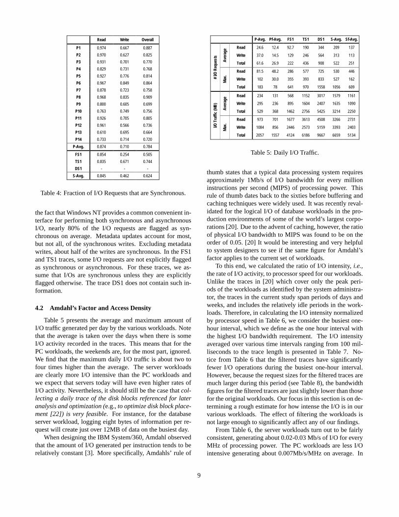
the fact that Windows NT provides a common convenient in-terface for performing both synchronous and asynchronousI/O, nearly 80% of the I/O requests are flagged as syn-chronous on average. Metadata updates account for most,but not all, of the synchronous writes. Excluding metadatawrites, about half of the writes are synchronous. In the FS1and TS1 traces, some I/O requests are not explicitly flaggedas synchronous or asynchronous. For these traces, we as-sume that I/Os are synchronous unless they are explicitlyflagged otherwise. The trace DS1 does not contain such in-formation.
4.2 Amdahl’s Factor and Access Density
Table 5 presents the average and maximum amount ofI/O traffic generated per day by the various workloads. Notethat the average is taken over the days when there is someI/O activity recorded in the traces. This means that for thePC workloads, the weekends are, for the most part, ignored.We find that the maximum daily I/O traffic is about two tofour times higher than the average. The server workloadsare clearly more I/O intensive than the PC workloads andwe expect that servers today will have even higher rates ofI/O activity. Nevertheless, it should still be the case thatcol-lecting a daily trace of the disk blocks referenced for lateranalysis and optimization (e.g.,to optimize disk block place-ment [22]) is very feasible. For instance, for the databaseserver workload, logging eight bytes of information per re-quest will create just over 12MB of data on the busiest day.
When designing the IBM System/360, Amdahl observedthat the amount of I/O generated per instruction tends to berelatively constant [3]. More specifically, Amdahls’ rule of
P-Avg. Pf-Avg. FS1 TS1 DS1 S-Avg. Sf-Avg.
Read 24.6 12.4 92.7 190 344 209 137
Write 37.0 14.5 129 246 564 313 113
Aver
age
Total 61.6 26.9 222 436 908 522 251
Read 81.5 48.2 286 577 725 530 446
Write 102 30.0 355 393 833 527 162#I/O
Requ
ests
Max
.
Total 183 78 641 970 1558 1056 609
Read 234 131 568 1152 3017 1579 1161
Write 295 236 895 1604 2407 1635 1090
Aver
age
Total 529 368 1462 2756 5425 3214 2250
Read 973 701 1677 3613 4508 3266 2731
Write 1084 856 2446 2573 5159 3393 2403I/OTr
affic
(MB)
Max
.
Total 2057 1557 4124 6186 9667 6659 5134
Table 5: Daily I/O Traffic.
thumb states that a typical data processing system requiresapproximately 1Mb/s of I/O bandwidth for every millioninstructions per second (MIPS) of processing power. Thisrule of thumb dates back to the sixties before buffering andcaching techniques were widely used. It was recently reval-idated for the logical I/O of database workloads in the pro-duction environments of some of the world’s largest corpo-rations [20]. Due to the advent of caching, however, the ratioof physical I/O bandwidth to MIPS was found to be on theorder of 0.05. [20] It would be interesting and very helpfulto system designers to see if the same figure for Amdahl’sfactor applies to the current set of workloads.
To this end, we calculated the ratio of I/O intensity,i.e.,the rate of I/O activity, to processor speed for our workloads.Unlike the traces in [20] which cover only the peak peri-ods of the workloads as identified by the system administra-tor, the traces in the current study span periods of days andweeks, and includes the relatively idle periods in the work-loads. Therefore, in calculating the I/O intensity normalizedby processor speed in Table 6, we consider the busiest one-hour interval, which we define as the one hour interval withthe highest I/O bandwidth requirement. The I/O intensityaveraged over various time intervals ranging from 100 mil-liseconds to the trace length is presented in Table 7. No-tice from Table 6 that the filtered traces have significantlyfewer I/O operations during the busiest one-hour interval.However, because the request sizes for the filtered traces aremuch larger during this period (see Table 8), the bandwidthfigures for the filtered traces are just slightly lower than thosefor the original workloads. Our focus in this section is on de-termining a rough estimate for how intense the I/O is in ourvarious workloads. The effect of filtering the workloads isnot large enough to significantly affect any of our findings.
From Table 6, the server workloads turn out to be fairlyconsistent, generating about 0.02-0.03 Mb/s of I/O for everyMHz of processing power. The PC workloads are less I/Ointensive generating about 0.007Mb/s/MHz on average. In
9

Avg. Number of Mbs of I/O Avg. Number of I/Os
PerSecond /s /MHz /s /MIPS /s /GB Per
Second /s /MHz /s /MIPS /s /GB
P1 0.588 0.00177 0.00177 0.0980 5.80 0.0174 0.0174 0.967
P2 0.557 0.00278 0.00278 0.116 7.25 0.0363 0.0363 1.51
P3 0.811 0.00180 0.00180 0.135 6.42 0.0143 0.0143 1.07
P4 6.84 0.0152 0.01520 1.14 61.0 0.135 0.135 10.2
P5 3.50 0.00778 0.00778 0.583 14.7 0.0326 0.0326 2.45
P6 0.106 0.000639 0.000639 0.0212 1.44 0.00866 0.00866 0.287
P7 2.84 0.0107 0.0107 0.711 28.5 0.107 0.107 7.13
P8 1.08 0.00361 0.00361 0.270 8.65 0.0288 0.0288 2.16
P9 1.11 0.00671 0.00671 0.371 15.4 0.0929 0.0929 5.14
P10 5.71 0.0215 0.0215 1.36 44.8 0.168 0.168 10.7
P11 0.852 0.00243 0.00243 0.213 10.9 0.0310 0.0310 2.72
P12 4.63 0.0116 0.0116 0.771 22.8 0.0570 0.0570 3.80
P13 0.385 0.00193 0.00193 0.0963 8.03 0.0401 0.0401 2.01
P14 4.14 0.00919 0.00919 0.517 51.8 0.115 0.115 6.47
P-Avg. 2.37 0.00697 0.00697 0.457 20.5 0.0632 0.0632 4.04
Pf-Avg. 1.92 0.00569 0.00569 0.372 9.24 0.0312 0.0312 1.94
FS1 1.26 0.0252 0.0503 0.419 26.8 0.536 1.07 8.94
TS1 1.99 0.0311 0.0621 0.191 39.0 0.610 1.22 3.75
DS1 6.11 0.0204 0.0407 0.117 72.4 0.241 0.482 1.38
S-Avg. 3.12 0.0255 0.0511 0.242 46.1 0.462 0.925 4.69
Sf-Avg. 2.98 0.0234 0.0467 0.217 29.5 0.375 0.750 3.99
Table 6: Intensity of I/O during the Busiest One-Hour Pe-riod.
order to determine an order of magnitude figure for the ratioof I/O bandwidth to MIPS, we need a rough estimate of theCycles Per Instruction (CPI) for the various workloads. Weuse a value of one for the PC workloads because the CPI forthe SPEC95 benchmark on the Intel Pentium Pro processorhas been found to be between 0.5 and 1.5 [6]. For the serverworkloads, we use a CPI value of two in view of results in[2, 25]. Based on this estimate of the CPI, we find that theserver workloads generate around 0.05 bits of real I/O perinstruction, which is consistent with the estimated Amdahl’sfactor for the production database workloads in [20].Thefigure for the PC workloads is seven times lower at about0.007 bits of I/O per instruction.
Interestingly, surveys of large data processing mainframeinstallations between 1980 and 1993 [33] found the numberof physical I/Os per second per MIPS to be decreasing byjust over 10% per year to 9.0 in 1993. This figure is aboutten times higher than what we are seeing for our server work-loads. A possible explanation for this large discrepancy isthat the mainframe workloads issue many small I/Os but thisturned out not to be true. Data reported in [33] show that theaverage I/O request size for the surveyed mainframe instal-lations was about 9KB, which is just slightly larger than the8KB for our server workloads (Table 8). Of course, main-frame MIPS and Reduced Instruction Set Computer (RISC)MIPS are not directly comparable and this difference couldaccount for some of the disparity, as could the inconsistentmethods used to calculate MIPS. The mainframe surveys
0.1s 1s 10s 1min 10min 1hr Trace Len.
P1 115 55.3 27.3 8.63 2.13 0.588 0.0366
P2 64.8 26.8 20.9 7.54 2.35 0.557 0.0234
P3 50.3 27.2 15.9 13.1 4.19 0.811 0.0129
P4 121 99.5 80.0 56.1 34.6 6.84 0.0893
P5 40.2 28.0 26.3 17.6 13.2 3.50 0.0674
P6 45.0 23.3 8.51 2.81 0.44 0.106 0.00549
P7 61.3 47.1 18.5 10.4 4.78 2.84 0.0463
P8 51.9 36.4 19.8 11.8 3.60 1.08 0.0204
P9 50.0 27.0 11.1 5.99 3.71 1.11 0.0306
P10 85.0 75.0 48.5 34.9 17.1 5.71 0.0358
P11 133 46.4 29.0 12.7 2.06 0.852 0.0266
P12 90.0 48.7 26.2 20.1 10.7 4.63 0.0139
P13 45.0 21.5 7.77 4.39 1.26 0.385 0.0148
P14 71.6 51.5 32.5 29.0 12.4 4.14 0.0476
P-Avg. 73.1 43.8 26.6 16.8 8.04 2.37 0.0337
Pf-Avg. 109 45 24.0 15.0 6.66 1.92 0.0237
FS1 382 41.1 26.1 11.9 2.05 1.26 0.133
TS1 264 96.3 14.9 10.8 4.88 1.99 0.260
DS1 156 108 91.9 85.1 19.7 6.11 0.515
S-Avg. 267 81.7 44.3 35.9 8.87 3.12 0.302
Sf-Avg. 262 76 42.9 32.0 7.71 2.98 0.213
Table 7: I/O Intensity (Mb/s) Averaged over Various TimeIntervals, showing the peak or maximum value observed foreach interval size.
used utilized MIPS [30] or the processing power actuallyconsumed by the workload. This is computed by factoringin the processor utilization when the workload is running.Our calculations are based on the MIPS rating of the system,which is what we have available to us. Ultimately though,we believe that intrinsic workload differences account fora major portion of the discrepancy between our results andthose from the mainframe surveys.
Another useful way of looking at I/O intensity is with re-spect to the storage used (Table 1). In this paper, the storageused by each of the workloads is estimated to be the com-bined size of all the file systems and logical volumes definedin that workload. This makes our calculations comparable tohistorical data and is a reasonable assumption unless storagecan be allocated only when written to, for instance by us-ing storage virtualization software that separates the systemview of storage from the actual physical storage. Table 6summarizes, for our various workloads, the number of I/Osper second per GB of storage used. This metric is commonlyreferred to as access density and is widely used in commer-cial data processing environments [33]. The survey of largedata processing mainframe installations cited above foundthe access density to be decreasing by about 10% per year to2.1 I/Os per second per GB of storage in 1993. Notice fromTable 6 that the access density for DS1 appears to be consis-tent with the mainframe survey results. However, the accessdensity for FS1 and TS1 is about two to four times higher.The PC workloads have, on average, an access density of 4I/Os per second per GB of storage, which is on the order of
10

All Requests Read Requests Write Requests
Avg. Std.Dev. Min. Max. Avg. Std.
Dev. Min. Max. Avg. Std.Dev. Min. Max.
P1 26 32.9 1 128 20.4 22.9 1 128 42.3 48.5 1 128
P2 19.7 30 1 1536 16.5 20.7 1 128 44.3 63.1 1 1536
P3 32.3 43.5 1 128 18.6 28.5 1 128 38.9 47.7 1 128
P4 28.7 40.2 1 128 15.5 21.1 1 128 29.8 41.2 1 128
P5 61 58.9 1 129 96.4 53.1 1 129 13 18.7 1 128
P6 18.9 29.4 1 128 27.6 29 1 128 16.8 29.1 1 128
P7 25.5 36.1 1 128 21.9 25 1 128 27.4 40.5 1 128
P8 32 42.6 1 128 21.2 31.5 1 128 55.3 52.9 1 128
P9 18.5 27.7 1 128 19.3 27.9 1 128 16 26.7 1 128
P10 32.6 44.4 1 128 37 46.4 1 128 23.1 37.8 1 128
P11 20.1 29 1 128 21.6 27.3 1 128 17.4 31.5 1 128
P12 51.9 120 1 512 96.4 144 1 512 38.2 107 1 512
P13 12.3 18.8 1 128 14.6 20.9 1 128 10.5 16.7 1 128
P14 20.5 38.6 1 128 13.7 29.1 1 128 72 58.3 1 128
P-Avg. 28.6 42.3 1 256 31.5 37.7 1 156 31.8 44.3 1 256
Pf-Avg. 55.5 93.3 1 512 34.2 38.2 1 155 91 141 1 512
FS1 12 5.52 2 18 11.6 5.61 2 18 14.4 4.15 2 16
TS1 13 9.87 2 512 12.6 5.52 2 64 14.9 19.9 2 512
DS1 21.6 35.3 1 128 25.4 38.6 1 108 19 32.5 1 128
S-Avg. 15.5 16.9 1.67 219 16.5 16.6 1.67 63.3 16.1 18.9 1.67 219
Sf-Avg. 25.8 12.7 2.00 213 27 8.73 2.00 51.3 13.1 13.4 2.67 213
Table 8: Request Size (Number of 512-Byte Blocks) duringthe Busiest One-Hour Period.
Processing Power (GHz) Storage (GB)Bandwidth(Mb/s) P-Avg. Pf-Avg. S-Avg. Sf-Avg. P-Avg. Pf-Avg. S-Avg. Sf-Avg.
Ethernet 10 0.718 0.879 0.196 0.214 10.9 13.4 20.6 23.0
Fast Ethernet 100 7.18 8.79 1.96 2.14 109 134 206 230
Gigabit Ethernet 1000 71.8 87.9 19.6 21.4 1093 1344 2063 2302
Ultra ATA-100 800 57.4 70.3 15.7 17.1 875 1075 1650 1842
Serial ATA 1200 86.1 105 23.5 25.7 1312 1613 2475 2763
UltraSCSI 320 2560 184 225 50.1 54.8 2799 3441 5281 5894
Fiber Channel 1000 71.8 87.9 19.6 21.4 1093 1344 2063 2302
Infiniband 2500 179 220 49.0 53.5 2733 3360 5157 5756
Table 9: Projected Processing Power and Storage Needed toDrive Various Types of I/O Interconnect to 50% Utilization.
the figure for the server workloads even though the serverworkloads are several years older. Such results suggest thatPC workloads may be comparable to server workloads interms of access density. Note, however, that as disks becomea lot bigger and PCs have at least one disk, the density ofaccess with respect to the available storage is likely to bemuch lower for PC workloads.
Table 6 also contains results for the number of bits ofI/O per second per GB of storage used. The PC work-loads have, on average, 0.46 Mb of I/O per GB of storage.By this measure, the server workloads are less I/O intensewith an average of only 0.24 Mb of I/O per GB of storage.Based on these results, we project the amount of processingpower and storage space that will be needed to drive varioustypes of I/O interconnect to 50% utilization. The results aresummarized in Table 9. Note that all the modern I/O inter-connects offer Gb/s bandwidth. Some of them, specifically
Inter-Arrival Time (s) P-Avg. Pf-Avg. FS1 TS1 DS1 S-Avg. Sf-Avg.
1st Moment 3.25 7.23 0.398 0.194 0.0903 0.227 0.561
2nd Moment 7.79E+05 1.86E+06 368 23.1 2.00 131 363
3rd Moment 6.46E+11 1.60E+12 2.02E+07 8.09E+03 67.4 6.74E+06 1.88E+07
Table 10: First, Second and Third Moments of the I/O Inter-Arrival Time.
0
20
40
60
80
100
1.E-05 1.E-04 1.E-03 1.E-02 1.E-01 1.E+00Inter-Arrival Time (s)
Cum
ulat
ive
%Ar
rival
s
P-Avg.
Pf-Avg.
S-Avg.
Sf-Avg.
P-Avg. - Exp. FitExp(0.233)
P-Avg.-FittedLognorm(0.175,7.58)
S-Avg.-FittedLognorm(0.315,0.227)
S-Avg. - Exp. FitExp(0.0914)
Figure 7: Distribution of I/O Inter-Arrival Time.
ethernet and fiber channel, have newer versions with evenhigher data rates. For the kinds of workloads that we have,the I/O interconnect is not expected to be a bottleneck anytime soon. However, we would expect to see much higherbandwidth requirements for workloads that are dominatedby large sequential I/Os (e.g., scientific and decision sup-port workloads [21]). In such environments, and especiallywhen many workloads are consolidated into a large serverand many disks are consolidated into a sizeable outboardcontroller, the bandwidth requirements have to be carefullyevaluated to ensure that the connection between the disksand the host does not become the bottleneck.
4.3 Request Arrival Rate
In Table 10, we present the first, second and third mo-ments of the inter-arrival time distribution. The distributionis plotted in Figure 7. Since the distribution of I/O inter-arrival time is often needed in modeling I/O systems, we fit-ted standard probability distributions to it. As shown in thefigure, the commonly used exponential distribution, whileeasy to work with mathematically, turns out to be a ratherpoor fit for all the workloads. Instead,the lognormal dis-tribution (denotedLognorm(µ, σ) whereµ and σ are re-spectively the mean and standard deviation) is a reasonably
11

# I/Os Outstanding # Reads Outstanding # Writes Outstanding
Avg. Avg.|>0 Std.Dev.
90%-tile Max. Avg. Avg.|>0 Std.
Dev.90%-tile Max. Avg. Avg.|>0 Std.
Dev.90%-tile Max.
P1 0.377 1.73 0.937 1 24 0.273 1.66 0.802 1 23 0.104 1.36 0.407 0 10
P2 0.421 1.9 1.01 2 13 0.28 1.93 0.864 1 12 0.141 1.45 0.473 0 6
P3 0.553 2.52 1.51 2 20 0.177 2.34 0.856 0 14 0.376 2.41 1.23 1 20
P4 0.796 2.67 1.96 3 74 0.332 2.15 1.1 1 27 0.464 2.33 1.55 1 74
P5 0.304 1.92 0.958 1 22 0.0985 1.97 0.601 0 20 0.206 1.71 0.704 1 22
P6 0.27 1.52 0.684 1 10 0.0169 1.36 0.181 0 8 0.253 1.52 0.66 1 8
P7 0.47 2.09 1.26 2 55 0.139 1.92 0.766 0 54 0.331 1.91 0.967 1 22
P8 0.365 1.96 1.07 1 26 0.196 1.65 0.699 1 14 0.168 1.82 0.673 0 16
P9 0.718 2.77 2.41 2 73 0.233 1.72 0.837 1 24 0.484 3.3 2.27 1 73
P10 0.573 2.33 1.81 2 60 0.252 1.62 0.766 1 19 0.321 2.53 1.62 1 60
P11 0.454 2.22 1.29 1 37 0.251 2.06 0.948 1 17 0.204 1.73 0.728 1 35
P12 0.341 1.99 1.06 1 19 0.201 2.37 0.897 0 17 0.14 1.35 0.464 1 8
P13 0.664 2.26 1.47 2 24 0.393 2.33 1.17 1 17 0.272 1.7 0.859 1 24
P14 0.541 2.11 1.28 2 23 0.184 1.62 0.677 1 17 0.358 1.98 1.05 1 23
P-Avg. 0.489 2.14 1.34 1.64 34.3 0.216 1.91 0.797 0.643 20.2 0.273 1.94 0.975 0.786 28.6
FS1 1.49 4.19 4.62 3 181 0.186 1.38 0.538 1 13 1.3 4.74 4.56 3 181
TS1 9.98 27.2 41.1 12 1530 0.214 1.42 0.574 1 20 9.76 36.4 41.1 11 1530
DS1 3.13 8.68 15.9 5 257 0.203 1.95 0.904 1 9 2.93 8.93 15.7 5 256
S-Avg. 4.87 13.4 20.5 6.67 656 0.201 1.58 0.672 1 14 4.66 16.7 20.5 6.33 656
Table 11: Queue Depth on Arrival.
good fit. Recall that a random variable is lognormally dis-tributed if the logarithm of the random variable is normallydistributed. Therefore, the lognormal distribution is skewedto the right or towards the larger values, meaning that thereexists long intervals with no I/O arrivals. The long tail ofthe inter-arrival distribution could be a manifestation of dif-ferent underlying behavior such as correlated arrival timesbut regardless of the cause, the net effect is thatI/O requestsseldom occur singly but tend to arrive in groupsbecause ifthere are long intervals with no arrivals, there must be in-tervals that have far more arrivals than their share. We willanalyze the burstiness of the I/O traffic in greater detail inthe next section.
Another interesting way to analyze the arrival process ofI/O requests is relative to the completion of preceding re-quests. In particular, if the workload supports multiple out-standing I/O requests, there will be more potential for im-proving the average I/O performance, for instance, throughrequest scheduling. Figure 8 presents the distribution ofqueue depth, which we define to be the length of the requestqueue as seen by an arriving request. In Table 11 and Fig-ure A-2 in Appendix A, we break down the outstanding re-quests into reads and writes. Note that we consider a requestto be in the queue while it is being serviced.
We find that across all the workloads, the read queuetends to be shallow - more than 85% of the requests arrive tofind the queue devoid of read requests, and the average num-ber of reads outstanding is only about 0.2. Nevertheless, theread queue can be deep at times. If there are read requestsin the queue, the average number of them is almost 2 (de-notedAvg.| > 0 in Table 11). In addition, the maximum
60
70
80
90
100
0 2 4 6 8 10 12 14 16 18 20Queue Depth on Arrival
Cum
ulat
ive
%of
Req
uest
s
P-Avg.
FS1
TS1
DS1
S-Avg.
Figure 8: Distribution of Queue Depth on Arrival. Bars in-dicate standard deviation.
12
read queue depth can be more than 90 times higher than theaverage. Notice thatthe server workloads do not appear tohave a deeper read queue than the personal system work-loads. This finding suggests that read performance in per-sonal system workloads could benefit as much from requestscheduling as in server workloads.We will examine this ingreater detail in [18]. Observe further from Table 11 thatthewrite queue is markedly deeper than the read queue for allthe workloads, as we would expect given that a greater frac-tion of writes are asynchronous compared to reads (Table 4).The PC workloads appear to have a significantly shallowerwrite queue than the other workloads but in most cases, thereare still enough outstanding write requests to benefit fromrequest scheduling.
Note that we are looking at the number of outstandingrequests from the perspective of the operating system layerat which the trace data were collected. This reflects the po-tential for request scheduling at any of the levels below, andnot just at the physical storage system, which is typically nothanded hundreds of requests at a time. Some of the differ-ences among the workloads could be the result of collectingthe traces at different levels on the different platforms. Ingeneral, the operating system and/or the disk device driverwill queue up the requests and attempt to schedule thembased on some simple performance model of the storage sys-tem (e.g.,minimize seek distance). There is a tendency forthe operating system and/or device driver to hold back therequests and issue only a small number of them at any onetime so as to avoid overloading the storage system. In real-ity, modern storage systems, specifically modern disks, havethe ability to do more elaborate and effective [54] requestscheduling based on whether a request will hit in the diskcache, and on the seek and rotational positions.
5 Variability in I/O Traffic over Time
When I/O traffic is smooth and uniform over time, systemresources can be very efficiently utilized. However, when theI/O traffic is bursty as is the case in practice (Section 4.3),resources have to be provisioned to handle the bursts so thatduring the periods when the system is relatively idle, theseresources will be wasted. There are several approaches totry to even out the load. The first is to aggregate multipleworkloads in the hope that the peak and idle periods in thedifferent workloads will tend to cancel out one another. Thisidea is one of the premises of the storage utilities model.Whether the aggregation of multiple workloads achieves thedesired effect of smoothening the load depends on whetherthe workloads are dependent or correlated. We will examinethe dependence among our workloads in Section 5.1.
The second approach to smoothening the traffic is to tryto shift the load temporally. For instance, by deferring oroffloading some work from the busy periods to the relativelulls (e.g.,write buffering and logging disk arrays [9, 50])
0
1
2
3
4
5
6
7
8
9
10
6 0 1 2 3 4 5 6 0 1 2 3 4 5 6 0 1 2 3 4 5 6 0 1 2 3 4 5 6 0 1 2 3 4 5 6 0 1 2 3 4 5 6 0 1Day of Week
Num
bero
fI/O
s(1
00,0
00s)
FS1
TS1
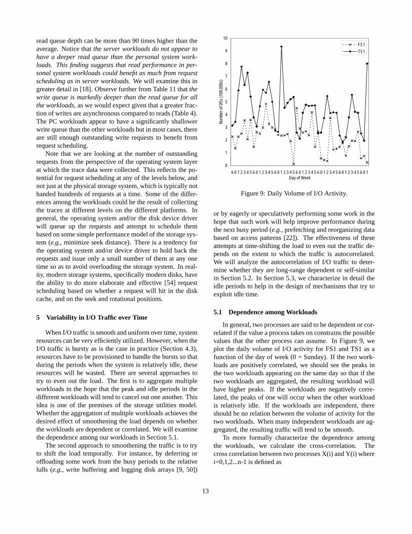
Figure 9: Daily Volume of I/O Activity.
or by eagerly or speculatively performing some work in thehope that such work will help improve performance duringthe next busy period (e.g.,prefetching and reorganizing databased on access patterns [22]). The effectiveness of theseattempts at time-shifting the load to even out the traffic de-pends on the extent to which the traffic is autocorrelated.We will analyze the autocorrelation of I/O traffic to deter-mine whether they are long-range dependent or self-similarin Section 5.2. In Section 5.3, we characterize in detail theidle periods to help in the design of mechanisms that try toexploit idle time.
5.1 Dependence among Workloads
In general, two processes are said to be dependent or cor-related if the value a process takes on constrains the possiblevalues that the other process can assume. In Figure 9, weplot the daily volume of I/O activity for FS1 and TS1 as afunction of the day of week (0 = Sunday). If the two work-loads are positively correlated, we should see the peaks inthe two workloads appearing on the same day so that if thetwo workloads are aggregated, the resulting workload willhave higher peaks. If the workloads are negatively corre-lated, the peaks of one will occur when the other workloadis relatively idle. If the workloads are independent, thereshould be no relation between the volume of activity for thetwo workloads. When many independent workloads are ag-gregated, the resulting traffic will tend to be smooth.
To more formally characterize the dependence amongthe workloads, we calculate the cross-correlation. Thecross correlation between two processes X(i) and Y(i) wherei=0,1,2...n-1 is defined as
13

86
88
90
92
94
96
98
100
1 10 100Avg. I/O Bandwidth during Interval (Normalized w.r.t Long-Run Avg.)
Cum
ulat
ive
%In
terv
als
P-Avg.Pf-Avg.FS1FS2TS1DS1S-Avg.Sf-Avg.
1-s Intervals
15
99
(a)
DS186
88
90
92
94
96
98
100
1 10 100I/O Bandwidth in Interval (Relative to Long-Run Average)
Cum
ulat
ive
%In
terv
als
0.1110100
Interval Size (s):
(b)
Figure 10: Distribution of I/O Traffic Averaged over Various Time Intervals.
rXY =∑
i (X(i)−X)(Y (i)− Y )√∑i(X(i)−X)2
√∑i(Y (i)− Y )2
(1)
The possible values ofRXY range from -1 to 1 with -1 in-dicating perfect negative correlation between the two work-loads, 0 no correlation, and 1 perfect positive correlation.For each workload, we consider the I/O arrival process ag-gregated over fixed intervals that range from one minute toa day. We synchronize the processes by the time of day andthe day of week. The results are available in Tables A-1 -A-4 in Appendix A.
To summarize the dependence among a set of workloadsW , we define the average cross-correlation asrXY whereX ∈ W , Y ∈ W andX 6= Y . In Figure A-3, we plot theaverage cross-correlation for the PC workloads as a functionof the time interval used to aggregate the arrival process. Inthe same figure, we also plot the average cross-correlationamong the server workloads. We find that, in general,thereis little cross-correlation among the server workloads, sug-gesting that aggregating them will likely help to smooth outthe traffic and enable more efficient utilization of resources.Our PC workloads are taken mostly from office environ-ments with flexible working hours. Neverthelessthe cross-correlation among the PC workloads is still significant ex-cept at small time intervals. This suggests that multiplexingthe PC workloads will smooth out the high frequency fluctu-ations in I/O traffic but some of the time-of-day effects willremain unless the PCs are geographically distributed in dif-
ferent time zones.Note that the filtered workloads tend to beless correlated but the difference is small.
5.2 Self-Similarity in I/O Traffic
In many situations, especially when outsourcing storage,we need rules of thumb to estimate the I/O bandwidth re-quirement of a workload without having to analyze the work-load in detail. In Section 4.2, we computed the access den-sity and found that the server workloads average about 5I/Os or about 30KB worth of I/O per second per GB of data.This result can be used to provide a baseline estimate forthe I/O bandwidth required by a workload given the amountof storage it uses. To account for the variability in the I/Otraffic, Figure 10(a) plots the distribution of I/O traffic aver-aged over one-second intervals and normalized to the aver-age bandwidth over the entire trace. The plot shows thattosatisfy the bandwidth requirement for 99% of the 1-secondintervals, we would need to provision for about 15 times thelong-run average bandwidth.Notice that for all the work-loads, there is an abrupt knee in the plots just beyond 99%of the intervals, which means thatto satisfy requirements be-yond 99% of the time will require disproportionately moreresources.
In analyzing the data, we noticed that for many of theworkloads, the distribution of I/O traffic is relatively insen-sitive to the size of the interval over which the traffic is aver-aged. For instance, in Figure 10(b), the distributions for timeintervals of 0.1s, 1s, 10s, 100s for the database server arevery similar. This scale-invariant characteristic is apparent
14

in Figure A-5, which shows the traffic variation over time fordifferent time scales for the time sharing and database serverworkloads. The topmost plot shows the throughput averagedover time intervals of 0.3s. In the second plot, we zoom outby a factor of ten so that each data point is the average trafficvolume over a three-second interval. The third plot zoomsout further by a factor of ten. Observe that rescaling the timeseries does not smooth out the burstiness. Instead the threeplots look similar. It turns out that for these workloads, suchplots look similar for time scales ranging from tens of mil-liseconds to tens of seconds.
Many of the statistical methods used in this section as-sume that the arrival process is stationary. In order to avoidpotential non-stationarity, we selected two one-hour periodsfrom each trace. The first period is chosen to be a high-traffic period, specifically one that contains more I/O trafficthan 95% of other one-hour periods in the trace. The secondperiod is meant to reflect a low traffic situation and is chosento be one that contains more I/O traffic than 30% of otherone-hour periods in the trace.
5.2.1 Definition of Self-Similarity
The phenomenon where a certain property of an objectis preserved with respect to scaling in space and/or timeis described by self-similarity and fractals [31]. LetXbe the incremental process of a processY , i.e., X(i) =Y (i + 1) − Y (i). In our case,Y counts the number of I/Oarrivals andX(i) is the number of I/O arrivals during theithtime interval. Y is said to be self-similar with parameterHif for all integersm,
X = m1−HX(m) (2)
where
X(m)(k) = (1/m)km∑
i=(k−1)m+1
X(i), k = 1, 2, ...
is the aggregated sequence obtained by dividing the orig-inal series into blocks of sizem and averaging over eachblock, andk is the index that labels each block. In this pa-per, we focus on second-order self-similarity, which meansthatm1−HX(m) has the same variance and autocorrelationasX. The interested reader is referred to [5] for a more de-tailed treatment.
The single parameterH expresses the degree of self-similarity and is known as the Hurst parameter. For smoothPoisson traffic, the H value is 0.5. For self-similar series,0.5 < H < 1, and asH → 1, the degree of self-similarityincreases. Mathematically, self-similarity is manifested inseveral equivalent ways and different methods that exam-ine specific indications of self-similarity are used to esti-mate the Hurst parameter. The interested reader is referredto Appendix B for details about how we estimate the degree
P-Avg. Pf-Avg. FS1 FS2 TS1 DS1 S-Avg. Sf-Avg.
H 0.81 0.79 0.88 0.92 0.91 0.91 0.90 0.80
ÿ (KB/s) 188 91.6 108 229 1000 445 367 1000
� 2 (KB/s)2 769080 528538 122544 345964 1256360 627261 528439 1256360
Table 12: Hurst Parameter, Mean and Variance of the Per-Second Traffic Arrival Rate during the High-Traffic Period.
of self-similarity for our various workloads. Here, we sim-ply summarize the Hurst parameter values we obtained (Ta-ble 12) and state the finding thatfor time scales ranging fromtens of milliseconds to tens and sometimes even hundreds ofseconds, the I/O traffic is well-represented by a self-similarprocess.Note that filtering the workloads does not affect theself-similar nature of their I/O traffic.
5.2.2 Implications of Self-Similar I/O Traffic
That the I/O traffic is self-similar implies that the bursti-ness exists over a wide range of time scales and that attemptsat evening out the traffic temporally will tend to not removeall the variability. In addition, the I/O system may experi-ence concentrated periods of congestion with associated in-crease in queuing time and that resource (e.g.,buffer, chan-nel) requirements may skyrocket at much lower levels of uti-lization than expected with the commonly assumed Poissonmodel in which arrivals are mutually independent and areseparated by exponentially distributed intervals. This behav-ior has to be taken into account when designing storage sys-tems, especially when we wish to isolate multiple workloadsso that they can coexist peacefully in the same storage sys-tem, as is required in many storage utilities. Such burstinessshould also be accounted for in the service level agreements(SLAs) when outsourcing storage.
More generally, I/O traffic has been known to be burstybut describing this variability has been difficult. The conceptof self-similarity provides us with a succinct way to char-acterize the burstiness of the traffic. We recommend thatI/O traffic be characterized by a three-tuple consisting of themean and variance of the arrival rate and some measure ofthe self-similarity of the traffic such as the Hurst parameter.The first two parameters can be easily understood and mea-sured. The third is more involved but can still be visuallyexplained. Table 12 summarizes these parameter values forour various workloads.
It turns out that self-similar behavior is not limited toI/O traffic or to our workloads. Recently, file system ac-tivities [15] and I/O traffic [13] have been found to ex-hibit scale-invariant burstiness. Local and wide-area net-work traffic may also be more accurately modeled using sta-tistically self-similar processes than the Poisson model(e.g.,[27]). However, analytical modeling with self-similar in-puts has not been well developed yet. (See [38] for some
15

-3
-2
-1
0
-2 -1 0 1 2log10(Length of On-Periods (s))
log 1
0(1-C
umul
ativ
e%
/100
)
1
2
3
4
5
slope=-2
slope=-1
I/O Rank of Process
P-Avg.
(a) On-Periods.
-4
-3
-2
-1
0
-1 0 1 2 3log10(Length of Off-Periods (s))
log 1
0(1-C
umul
ativ
e%
/100
)
1
2
3
4
5
slope=-2
slope=-1
I/O Rank of Process
P-Avg.
(b) Off-Periods.
Figure 11: Length of On/Off Periods for the Five Most I/O-Active Processes.
recent results on modeling network traffic with self-similarprocesses). This, coupled with the complexity of storagesystems today, means that most of the analysis has to beperformed through simulations. Generating I/O traffic thatis consistent with the self-similar characteristic observed inreal workloads is therefore extremely important and useful.In Appendix B, we present a recipe that can be used to gen-erate self-similar traffic using the parameters in Table 12.
5.2.3 Underpinnings of Self-Similar I/O Traffic
We have seen that I/O traffic is self-similar but self-similarity is a rather abstract concept. To present a morecompelling case and provide further insights into the dy-namic nature of the traffic, we try to relate this phenomenonto some underlying physical cause, namely the superpositionof I/O from multiple processes in the system where each pro-cess behaves as an independent source of I/O with on periodsthat are heavy-tailed.
A random variable,X, is said to follow a heavy-taileddistribution if
P (X > x) ∼ cx−α, as x →∞, c > 0, 1 < α < 2. (3)
Such a random variable can give rise to extremely large val-ues with non-negligible probability. The superposition of alarge number of independent traffic sources with on and/oroff periods that are heavy-tailed is known to result in trafficthat is self-similar1 [53]. In this section, we break down each
1Not Poisson; assumptions of Palm-Khintchine theorem are notsatisfied.
workload into the I/O traffic generated by the individual pro-cesses. As in [13], we define an off period for a process asany interval longer than 0.2s during which the process doesnot generate any I/O. All other intervals are considered onperiods for the process. This analysis has been shown to berelatively insensitive to the threshold value used to distin-guish the on and off periods [53].
Taking logarithm on both sides of Equation 3, we get
logP (X > x) ∼ log(c)− αlog(x), as x →∞. (4)
Therefore, ifX is heavy-tailed, the plot ofP (X > x) versusx on log-log scale should yield a straight line with slopeαfor large values ofx. Such log-log plots are known as com-plementary cumulative distribution plots or “qq-plots” [26].In Figure 11, we present the qq-plots for the lengths of theon and off periods for the five processes that generate themost I/O traffic in each of our PC workloads. Unfortunately,none of our other workloads contain the process informa-tion that is needed for this analysis. As shown in the figure,the on periods appear to be heavy-tailed but not the off peri-ods. This is consistent with results reported in [13] where thelack of heavy-tailed behavior for the off periods is attributedto periodic activity such as the sync daemon traffic. Hav-ing heavy-tailed on periods is sufficient, however, to resultin self-similar aggregate traffic.
5.3 The Relative Lulls
As discussed earlier, when the I/O load is not constantbut varies over time, there may be opportunities to use the
16

0
20
40
60
80
100
1.E+01 1.E+02 1.E+03 1.E+04Duration of Idle Period (s)
Cum
ulat
ive
%Id
lePe
riods
P-Avg.
Pf-Avg.
FS1
DS1
S-Avg.
Sf-Avg.
P-Avg.-Fitted
Lognorm(5.72x103,1.23x105)
S-Avg.-Fitted
Lognorm(655,4.84x103)
(a)
0
20
40
60
80
100
1.E+01 1.E+02 1.E+03 1.E+04 1.E+05Duration of Idle Period (s)
Cum
ulat
ive
%Id
lePe
riods
(Wei
ghte
d)
P-Avg.
Pf-Avg.
FS1
DS1
S-Avg.
Sf-Avg.
P-Avg.-Fitted
Lognorm(6.16x105,4.83x106)
S-Avg.-Fitted
Lognorm(1.74x104,9.75x104)
(b)
Figure 12: Distribution of Idle Period Duration. For the weighted distribution in (b), an idle period of durations is countedstimes,i.e., it is the distribution of idle time.
relatively idle periods to do some useful work. The readeris referred to [12] for an overview of idle-time processingand a general taxonomy of idle-time detection and predictionalgorithms. Here, we characterize in detail the idle periods,focusing on specific metrics that will be helpful in designingmechanisms that try to exploit idle time.
We consider an interval to be idle if the average num-ber of I/Os per second during the interval is less than somevaluek. The term idle period refers to a sequence of inter-vals that are idle. The duration of an idle period is simplythe product of the number of idle intervals it contains andthe interval size. In this study, we use a relatively long in-terval of 10 seconds because we are interested in long idleperiods during which we can perform a substantial amountof work. Note that storage systems tend to have some pe-riodic background activity so that treating an interval to beidle only if it contains absolutely no I/O activity would befar too conservative. Since disks today are capable of sup-porting in excess of 100 I/Os per second [18], we selectkto be 20 for all our workloads except DS1. DS1 containsseveral times the allocated storage in the other workloads soits storage system will presumably be much more powerful.Therefore, we use ak value of 40 for DS1.
Figure 12 presents the distribution of idle period durationfor our workloads. We fitted standard probability distribu-tions to the data and found that the lognormal distribution isa reasonably good fit for most of the workloads. Notice thatalthough most of the idle periods are short (less than a hun-dred seconds), long idle periods account for most of the idle
time. This is consistent with previous results and implies thata system that exploits idle time can get most of the potentialbenefit by simply focusing on the long idle periods[12].
5.3.1 Inter-idle Gap
An important consideration in attempting to make use ofidle periods is the frequency with which suitably long idleperiods can be expected. In addition, the amount of activitythat occurs between such long idle periods also determinesthe effectiveness and even the feasibility of exploiting theidle periods. For instance, a log-structured file system orarray [34, 44] where garbage collection is performed peri-odically during system idle time may run out of free spaceif there is a lot of write activity between the idle periods. Inthe disk block reorganization scheme proposed in [22], theinter-idle gap,i.e., the time span between suitably long idleperiods, determines the amount of reference data that has tobe accumulated on the disk.
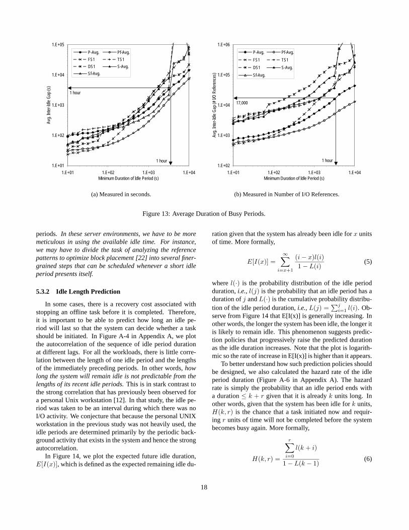
In Figure 13, we consider this issue by plotting the aver-age inter-idle gap as a function of the duration of the idle pe-riod. The results show that for the PC workloads on average,idle periods lasting at least an hour are separated by busyperiods of about an hour and with just over 17,000 refer-ences. These results indicate thatin the personal systems en-vironment, there are long idle periods that occur frequentlyenough to be interesting for offline optimizations such asblock reorganization[22]. As we would expect, the serverworkloads have longer busy periods separated by shorter idle
17
1.E+01
1.E+02
1.E+03
1.E+04
1.E+05
1.E+01 1.E+02 1.E+03 1.E+04Minimum Duration of Idle Period (s)
Avg.
Inte
r-Idl
eG
ap(s
)P-Avg. Pf-Avg.
FS1 TS1
DS1 S-Avg.
Sf-Avg.
1 hour
1 hour
(a) Measured in seconds.
1.E+02
1.E+03
1.E+04
1.E+05
1.E+06
1.E+01 1.E+02 1.E+03 1.E+04Minimum Duration of Idle Period (s)
Avg.
Inte
r-Idl
eG
ap(#
I/OR
efer
ence
s)
P-Avg. Pf-Avg.
FS1 TS1
DS1 S-Avg.
Sf-Avg.
1 hour
17,000
(b) Measured in Number of I/O References.
Figure 13: Average Duration of Busy Periods.
periods. In these server environments, we have to be moremeticulous in using the available idle time. For instance,we may have to divide the task of analyzing the referencepatterns to optimize block placement [22] into several finer-grained steps that can be scheduled whenever a short idleperiod presents itself.
5.3.2 Idle Length Prediction
In some cases, there is a recovery cost associated withstopping an offline task before it is completed. Therefore,it is important to be able to predict how long an idle pe-riod will last so that the system can decide whether a taskshould be initiated. In Figure A-4 in Appendix A, we plotthe autocorrelation of the sequence of idle period durationat different lags. For all the workloads, there is little corre-lation between the length of one idle period and the lengthsof the immediately preceding periods. In other words,howlong the system will remain idle is not predictable from thelengths of its recent idle periods.This is in stark contrast tothe strong correlation that has previously been observed fora personal Unix workstation [12]. In that study, the idle pe-riod was taken to be an interval during which there was noI/O activity. We conjecture that because the personal UNIXworkstation in the previous study was not heavily used, theidle periods are determined primarily by the periodic back-ground activity that exists in the system and hence the strongautocorrelation.
In Figure 14, we plot the expected future idle duration,E[I(x)], which is defined as the expected remaining idle du-
ration given that the system has already been idle forx unitsof time. More formally,
E[I(x)] =∞∑
i=x+1
(i− x)l(i)1− L(i)
(5)
wherel(·) is the probability distribution of the idle periodduration,i.e., l(j) is the probability that an idle period has aduration ofj andL(·) is the cumulative probability distribu-tion of the idle period duration,i.e.,L(j) =
∑ji=1 l(i). Ob-
serve from Figure 14 that E[I(x)] is generally increasing. Inother words, the longer the system has been idle, the longer itis likely to remain idle. This phenomenon suggests predic-tion policies that progressively raise the predicted durationas the idle duration increases. Note that the plot is logarith-mic so the rate of increase in E[I(x)] is higher than it appears.
To better understand how such prediction policies shouldbe designed, we also calculated the hazard rate of the idleperiod duration (Figure A-6 in Appendix A). The hazardrate is simply the probability that an idle period ends witha duration≤ k + r given that it is alreadyk units long. Inother words, given that the system has been idle fork units,H(k, r) is the chance that a task initiated now and requir-ing r units of time will not be completed before the systembecomes busy again. More formally,
H(k, r) =
r∑i=0
l(k + i)
1− L(k − 1)(6)
18

0
20000
40000
60000
80000
100000
120000
0 5000 10000 15000 20000Idle Duration (s)
Expe
cted
Rem
aini
ngId
leD
urat
ion
(s)
P-Avg.
Pf-Avg.
0
5000
10000
15000
20000
25000
30000
0 5000 10000 15000 20000Idle Duration (s)
Expe
cted
Rem
aini
ngId
leD
urat
ion
(s)
FS1
TS1
DS1
S-Avg.
Sf-Avg.
Figure 14: Remaining Idle Duration.
We find that the hazard rate is generally declining as theidle period duration increases.This result again supportsthe idea of predicting idle period duration by conditioningon the amount of time the system has already been idle.Inaddition, the hazard rate increases withr, which is what wewould expect. In other words, the chances that a task willnot be completed before the system becomes busy again in-creases with the length of the task.
6 Interaction of Reads and Writes
In general, the interaction between reads and writes com-plicates a computer system and throttles its performance.For instance, static data can be simply replicated to improvenot only the performance of the system but also its scalabilityand durability. But if the data is being updated, the systemhas to ensure that the writes occur in the correct order. Inaddition, it has to either propagate the results of each writeto all possible replicated copies or to invalidate these copies.The former usually makes sense if the updated data is un-likely to be updated again but is likely to be read. The latteris useful when it is highly likely that the data will be updatedseveral more times before it is read. In cases where the datais being both updated and read, replication may not be use-ful. Thus the read-write composition of the traffic, togetherwith the flow of data from writes to reads, is an extremelyimportant workload characteristic. This is the focus of thissection.
6.1 Read/Write Ratio
A wide range of read/write ratio has been reported inthe literature. In addition to intrinsic workload differences,
the read-to-write ratio also depends a lot on how much ofthe reads and writes have been filtered by caching, and onthe kinds of I/Os (e.g.,user data, paging, file system meta-data) that are tabulated. Because main memory is volatile,the amount of write buffering performed by the file systemcache is typically limited. For example, UNIX systems havetraditionally used a policy of periodically (once every 30s)flushing the dirty blocks in the file cache to disk so as tolimit the amount of data that will potentially be lost in a sys-tem failure. In Windows NT, one quarter of the dirty datain the file cache is written back to disk every second [46].Therefore, more of the reads than writes are filtered by thefile system cache. The file system also adds metadata writeswhich can account for more than half of the physical writes(more than 72% in [45] and more than 53% in our PC work-loads). Therefore, at the logical level, the read/write ratio isgenerally much higher than at the physical level.
For instance, the ratio of logical read to write traffic hasbeen reported to be between 3.7 and 6.3 for desktop work-station workloads [42], and the ratio of logical read to writeoperations has been found to be between 3 and 4.5 in var-ious office environments [41]. At the physical level, theread/write ratio has been observed to range from about 0.4 to1 for Novell NetWare file servers [17] and from about 0.7 to0.8 for several HP-UX systems [45]. These figures are com-parable to the read/write ratio we obtained, which are pre-sented in Table 13. Observe thatconsistently across all theserver workloads and the PC workloads, on average, writesaccount for about 60% of the requests. Interestingly, main-frame data processing workloads appear to have a higherread/write ratio. For example, measurements conducted atthe physical level at 12 moderate-to-large MVS installationsrunning mainly data processing applications (circa 1993)
19

Requests
RequestsWrite#
RequestsRead#
Traffic
WrittenMB
ReadMB
Footprint
WrittenBlocksUnique#
ReadBlocksUnique#
P1 2.51 1.99 1.05
P2 1.37 1.79 1.55
P3 0.429 0.430 0.563
P4 0.606 0.550 0.585
P5 0.338 0.475 1.02
P6 0.147 0.231 0.322
P7 0.288 0.299 0.399
P8 1.23 1.14 0.941
P9 0.925 1.02 1.38
P10 0.937 1.41 2.17
P11 0.831 1.38 0.787
P12 0.758 0.883 0.904
P13 0.566 0.744 1.40
P14 0.481 0.710 0.770
P-Avg. 0.816 0.932 0.988
Pf-Avg. 0.965 0.607 0.888
FS1 0.718 0.633 1.50
TS1 0.794 0.740 1.15
DS1 0.607 1.24 1.06
S-Avg. 0.706 0.870 1.24
Sf-Avg. 1.12 0.843 1.19
Table 13: Read/Write Ratio.
found the read/write ratio to be about 3.5 [33]. Analysisof the logical I/O traffic of the production database work-loads of ten of the world’s largest corporations of aboutthe same period found the read/write ratio to average about10 [20, 21].
Observe from Table 13 that for the PC workloads, theread/write ratio does appear to be negatively correlated withthe memory size of the system. Unfortunately, we do nothave enough data points to observe any trends for the serverworkloads. In Figure 15, we plot the read/write ratio for thePC workloads as a function of the memory size. As shownin the figure, the read/write ratio is approximately relatedto the memory size by an exponential function of the formf(x) = aeb/x wherea andb are constants. The model islimited by the few data points we have but it predicts thatwith an infinitely large memory,i.e., asx → ∞, there willbe about 6 writes for every read. Such results support to theprediction that almost all reads will be absorbed by the largerbuffer caches in the future so that physical I/O will becomedominated by writes [36, 37, 44]. However, that the readratio remains relatively consistent across all our workloads,which span a time period of eight years, suggests that work-load changes may have a counter effect. Also, the fact thatthe ratio of read footprint to write footprint decreases, albeitslowly, with memory size, suggests that effects (e.g.,work-load differences) other than an increase in caching, couldalso be at work here.
0
0.5
1
1.5
2
2.5
3
0 64 128 192 256Memory Size (MB)
Rea
d/W
rite
Rat
io
Requests
Traffic
FootprintFootprint - Fitted
f(x) = 0.628e43.0/x
r2=0.126
Traffic - Fitted
f(x) = 0.241e121/x
r2=0.720
Requests - Fitted
f(x) = 0.164e141/x
r2=0.607
Figure 15: Read/Write Ratio as Function of Memory Size.
If writes become increasingly dominant, a pertinent ques-tion to ponder is whether physical read performance reallymatters. In Figure 16, we plot the read and write cache missratios assuming a write-back cache with the least-recently-used (LRU) cache replacement policy. We define the missratio to be the fraction of requests that are not filtered by thecache but that result in a request to the underlying storagesystem. Observe that the plots for the filtered workloads aresimply a translation of those for the original workloads; thebehavior is qualitatively similar. Note that we are in essencesimulating a second level cache. The upstream file systemcache and/or the database buffer pool have captured signifi-cant portions of any read reuse but because they are volatile,they cannot safely cache the writes. Therefore, thewritesobserved at the storage level exhibit much stronger local-ity than the reads. In other words, although read cachingby the file system or the database buffer can eliminate mostof the reads, if writes are delayed long enough by usingnon-volatile memory, write requests can similarly be verysignificantly reduced. In fact, for practically all the work-loads, a small cache of 1MB eliminates more than half thewrites. Furthermore, unlike reads which tend to be syn-chronous, writes can be effectively rendered asynchronousthrough the use of write caching. In addition, the effec-tive latency of writes can often be reduced by writing dataasynchronously or in a log [44, 52] or by using write-aheadlogging [35]. Recent results (e.g.,[10]) also suggest that be-cause of the widening performance gap between processorand disk-based storage, file system read response times maybe dominated by disk accesses even at very high cache hitrates. Therefore,the performance of read I/Os continues tobe very important.
20
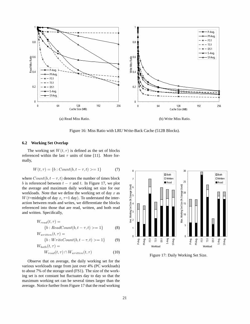
0
0.2
0.4
0.6
0.8
1
0 64 128 192 256Cache Size (MB)
Rea
dM
iss
Rat
io
P-Avg.
Pf-Avg.
FS1
TS1
DS1
S-Avg.
Sf-Avg.
(a) Read Miss Ratio.
0
0.2
0.4
0.6
0.8
1
0 64 128 192 256Cache Size (MB)
Writ
eM
iss
Rat
io
P-Avg.
Pf-Avg.
FS1
TS1
DS1
S-Avg.
Sf-Avg.
(b) Write Miss Ratio.
Figure 16: Miss Ratio with LRU Write-Back Cache (512B Blocks).
6.2 Working Set Overlap
The working setW (t, τ) is defined as the set of blocksreferenced within the lastτ units of time [11]. More for-mally,
W (t, τ) = {b : Count(b, t− τ, t) >= 1} (7)
whereCount(b, t− τ, t) denotes the number of times blockb is referenced betweent − τ andt. In Figure 17, we plotthe average and maximum daily working set size for ourworkloads. Note that we define the working set of dayx asW (t=midnight of dayx, τ=1 day). To understand the inter-action between reads and writes, we differentiate the blocksreferenced into those that are read, written, and both readand written. Specifically,
Wread(t, τ) ={b : ReadCount(b, t− τ, t) >= 1} (8)
Wwritten(t, τ) ={b : WriteCount(b, t− τ, t) >= 1} (9)
Wboth(t, τ) =Wread(t, τ) ∩Wwritten(t, τ) (10)
Observe that on average, the daily working set for thevarious workloads range from just over 4% (PC workloads)to about 7% of the storage used (FS1). The size of the work-ing set is not constant but fluctuates day to day so that themaximum working set can be several times larger than theaverage. Notice further from Figure 17 that the read working
0
1
2
3
4
5
6
7
8
P-Av
g.
Pf-A
vg.
FS1
TS1
DS1
S-Av
g
Sf-A
vg.
Workload
Ave.
Wor
king
SetS
ize
(%St
orag
eU
sed)
Both
Written
Read
0
5
10
15
20
25
30
P-Av
g.
Pf-A
vg.
FS1
TS1
DS1
S-Av
g.
Sf-A
vg.
Workload
Max
.Wor
king
SetS
ize
(%St
orag
eU
sed)
Both
Written
Read
Figure 17: Daily Working Set Size.
21
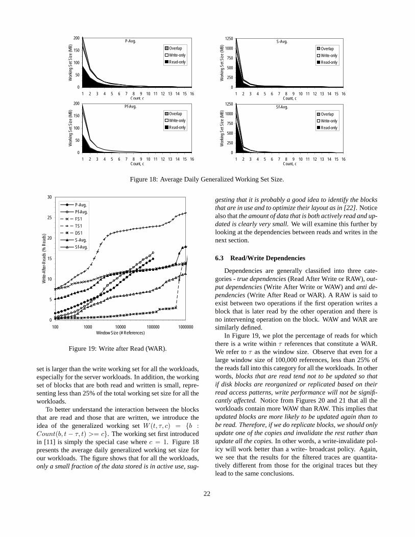
P-Avg.
0
50
100
150
200
1 2 3 4 5 6 7 8 9 10 11 12 13 14 15 16Count, c
Wor
king
SetS
ize
(MB) Overlap
Write-only
Read-only
S-Avg.
0
250
500
750
1000
1250
1 2 3 4 5 6 7 8 9 10 11 12 13 14 15 16Count, c
Wor
king
SetS
ize
(MB) Overlap
Write-only
Read-only
Pf-Avg.
0
50
100
150
200
1 2 3 4 5 6 7 8 9 10 11 12 13 14 15 16Count, c
Wor
king
SetS
ize
(MB) Overlap
Write-only
Read-only
Sf-Avg.
0
250
500
750
1000
1250
1 2 3 4 5 6 7 8 9 10 11 12 13 14 15 16Count, c
Wor
king
SetS
ize
(MB) Overlap
Write-only
Read-only
Figure 18: Average Daily Generalized Working Set Size.
0
5
10
15
20
25
30
100 1000 10000 100000 1000000Window Size (# References)
Writ
e-Af
ter-R
eads
(%R
eads
)
P-Avg.
Pf-Avg.
FS1
TS1
DS1
S-Avg.
Sf-Avg.
Figure 19: Write after Read (WAR).
set is larger than the write working set for all the workloads,especially for the server workloads. In addition, the workingset of blocks that are both read and written is small, repre-senting less than 25% of the total working set size for all theworkloads.
To better understand the interaction between the blocksthat are read and those that are written, we introduce theidea of the generalized working setW (t, τ, c) = {b :Count(b, t − τ, t) >= c}. The working set first introducedin [11] is simply the special case wherec = 1. Figure 18presents the average daily generalized working set size forour workloads. The figure shows that for all the workloads,only a small fraction of the data stored is in active use, sug-
gesting that it is probably a good idea to identify the blocksthat are in use and to optimize their layout as in [22]. Noticealso thatthe amount of data that is both actively read and up-dated is clearly very small.We will examine this further bylooking at the dependencies between reads and writes in thenext section.
6.3 Read/Write Dependencies
Dependencies are generally classified into three cate-gories -true dependencies(Read After Write or RAW),out-put dependencies(Write After Write or WAW) andanti de-pendencies(Write After Read or WAR). A RAW is said toexist between two operations if the first operation writes ablock that is later read by the other operation and there isno intervening operation on the block. WAW and WAR aresimilarly defined.
In Figure 19, we plot the percentage of reads for whichthere is a write withinτ references that constitute a WAR.We refer toτ as the window size. Observe that even for alarge window size of 100,000 references, less than 25% ofthe reads fall into this category for all the workloads. In otherwords,blocks that are read tend not to be updated so thatif disk blocks are reorganized or replicated based on theirread access patterns, write performance will not be signifi-cantly affected.Notice from Figures 20 and 21 that all theworkloads contain more WAW than RAW. This implies thatupdated blocks are more likely to be updated again than tobe read. Therefore, if we do replicate blocks, we should onlyupdate one of the copies and invalidate the rest rather thanupdate all the copies.In other words, a write-invalidate pol-icy will work better than a write- broadcast policy. Again,we see that the results for the filtered traces are quantita-tively different from those for the original traces but theylead to the same conclusions.
22

0
10
20
30
40
100 1000 10000 100000 1000000Window Size (# References)
Rea
d-Af
ter-W
rites
(%W
rites
)P-Avg.
Pf-Avg.
FS1
TS1
DS1
S-Avg.
Sf-Avg.
Figure 20: Read after Write (RAW).
7 Conclusions
In this paper, we empirically analyze the I/O traffic of awide range of real workloads with an emphasis on under-standing how these workloads will respond to new storagedevelopments such as network storage, storage utilities, andintelligent self-optimizing storage. As part of our analysis,we also study the effect of increased upstream caching onthe traffic characteristics seen by the storage system and dis-cover that it affects our analysis only quantitatively. Our ma-jor findings include:
• Importance of I/O Innovation/Optimization
I/O is known to be a major component of server work-loads and improving the I/O performance for theseworkloads is critical. Our results suggest that if pro-cessors continue to increase in performance accordingto Moore’s Law, I/O is likely to also become a domi-nant component of personal computer workloads in thenext few years. Our data show that consistently acrossall the workloads, writes account for about 60% of therequests. However, just as read caching by the file sys-tem or the database buffer can eliminate most of thereads, if writes are delayed long enough by using non-volatile memory, write requests can similarly be verysignificantly reduced. In fact, for practically all theworkloads, a small write-back cache of 1MB eliminatesmore than half the writes. We believe that the perfor-mance of read I/Os is likely to continue to have a di-rect impact on application performance. As part of ouranalysis, we re-examined Amdahl’s rule of thumb fora balanced system and found that our server workloadsgenerate on the order of 0.05 bits of physical I/O perinstruction, consistent with our earlier work using the
0
20
40
60
80
100
100 1000 10000 100000 1000000Window Size (# References)
Writ
e-Af
ter-W
rites
(%W
rites
)
P-Avg.
Pf-Avg.
FS1
TS1
DS1
S-Avg.
Sf-Avg.
Figure 21: Write after Write (WAW).
production database workloads of some of the world’slargest corporations [20]. The figure for the PC work-loads is seven times lower at about 0.007 bits of physi-cal I/O per instruction.
• Burstiness of I/O Traffic
Across all the workloads, read and write I/O requestsseldom occur singly but tend to arrive in groups. Wefind that the write queue is very much deeper than theread queue. Our analysis also indicates that there is lit-tle cross-correlation in traffic volume among the serverworkloads, suggesting that aggregating them will likelyhelp to smooth out the traffic and enable more efficientutilization of resources. As for the PC workloads, mul-tiplexing them will remove the high frequency fluctua-tions in I/O traffic but some of the time-of-day effectsare likely to remain unless the PCs are geographicallydistributed in different time zones. In addition, our re-sults also show that to satisfy I/O bandwidth require-ments 99% of the time, we will need to provision for15 times the long-run average bandwidth. Going be-yond 99% of the time will require disproportionatelymore resources. It turns out that for time scales rangingfrom tens of milliseconds to tens and sometimes evenhundreds of seconds, the I/O traffic is well-representedby a self-similar process. This implies that the I/O sys-tem may become overwhelmed at much lower levels ofutilization than expected with the commonly assumedPoisson model. Such behavior has to be taken into ac-count when designing storage systems, and in the ser-vice level agreements (SLAs) when outsourcing stor-age. We recommend that I/O traffic be characterized by
23

a three-tuple consisting of the mean and variance of thearrival rate, and the Hurst parameter.
• Potential for Harnessing “Free” Resources
We find that our PC workloads contain a lot of pro-cessor idle time for performing background tasks, evenwithout having to deliberately leave the computer onwhen the user is away. The storage system is also rela-tively idle. For all the workloads, a system that exploitsidle time can get most of the potential benefit by simplyfocusing on the long idle periods. In the personal sys-tems environment, there are idle periods that are bothlong enough and that occur frequently enough to be in-teresting for offline optimizations such as block reorga-nization. In the server environment, we have to be moremeticulous in using the available idle time, for instance,by dividing an idle-time task into several finer-grainedsteps that can be scheduled whenever a short idle pe-riod presents itself. Our results suggest that the lengthof an idle period can be predicted more accurately byconditioning on the amount of time the system has al-ready been idle than from the lengths of the recent idleperiods.
• Opportunity for Block Reorganization
In general, I/O traffic is low enough for it to be feasi-ble to collect a daily trace of the blocks referenced forlater analysis and optimization. We discover that onlya small fraction of the data stored is in active use, sug-gesting that it is probably a good idea to identify theblocks that are in use and to optimize their layout. Inaddition, the amount of data that is both actively readand updated is very small. Moreover, blocks that areread tend not to be updated so that if blocks are reor-ganized or replicated based on their read access pat-terns, write performance will not be significantly af-fected. Because updated blocks are more likely to beupdated again than to be read, if blocks are replicated,a write-invalidate policy will tend to work better than awrite-broadcast policy.
8 Acknowledgements
The authors would like to thank Ruth Azevedo, CarlosFuente, Jacob Lorch, Bruce McNutt, Anjan Sen and JohnWilkes for providing the traces used in this study. In addi-tion, the authors are grateful to Jai Menon, John Palmer andHonesty Young for helpful comments on versions of this pa-per.
References
[1] P. Abry and D. Veitch, “Wavelet analysis oflong-range-dependent traffic,”IEEE Transactions onInformation Theory, 44, 1, pp. 2–15, 1998.
[2] A. Ailamaki, D. J. DeWitt, M. D. Hill, and D. A. Wood,“DBMSs on a modern processor: Where does time go,”Proceedings of International Conference on Very Large DataBases (VLDB), (Edinburgh, Scotland), Sept. 1999.
[3] G. M. Amdahl, “Storage and I/O parameters and systemspotential,”Proceedings of IEEE International ComputerGroup Conference (Memories, Terminals, and Peripherals),(Washington, DC), pp. 371–372, June 1970.
[4] M. G. Baker, J. H. Hartman, M. D. Kupfer, K. W. Shirriff,and J. K. Ousterhout, “Measurements of a distributed filesystem,”Proceedings of ACM Symposium on OperatingSystems Principles (SOSP), (Pacific Grove, CA),pp. 198–212, Oct. 1991.
[5] J. Beran,Statistics for Long-Memory Processes, Chapman &Hall, New York, NY, 1994.
[6] D. Bhandarkar and J. Ding, “Performance characterization ofthe Pentium Pro processor,”Proceedings of ThirdInternational Symposium on High-Performance ComputerArchitecture (HPCA), (San Antonio, Texas), pp. 288–297,Feb. 1997.
[7] P. Biswas, K. K. Ramakrishnan, and D. Towsley, “Tracedriven analysis of write caching policies for disks,”Proceedings of ACM Conference on Measurement andModeling of Computer Systems (SIGMETRICS), (SantaClara, CA), pp. 13–23, May 1993.
[8] G. P. Bozman, H. H. Ghannad, and E. D. Weinberger, “Atrace-driven study of CMS file references,”IBM Journal ofResearch and Development, 35, 5/6, pp. 815–828, Sept./Nov.1991.
[9] Y. Chen, W. W. Hsu, and H. C. Young, “Logging RAID - anapproach to fast, reliable, and low-cost disk arrays,”Proceedings of European Conference on Parallel Computing(EuroPar), (Munich, Germany), Aug. 2000.
[10] M. Dahlin,Serverless Network File Systems, PhD thesis,University of California, Berkeley, Dec. 1995.
[11] P. J. Denning, “The working set model for programbehaviour,”Communications of the ACM, 11, 5, May 1968.
[12] R. Golding, P. Bosch, C. Staelin, T. Sullivan, and J. Wilkes,“Idleness is not sloth,”Proceedings of USENIX TechnicalConference, (New Orleans, LA), pp. 201–212, Jan. 1995.Extended version available as Technical Report HPL-96-140,HP Laboratories, Palo Alto, CA, Oct. 1996.
[13] M. E. Gomez and V. Santonja, “Analysis of self-similarity inI/O workload using structural modeling,”Proceedings of 7thSymposium on Modeling, Analysis and Simulation ofComputer and Telecommunication Systems (MASCOTS),(College Park, MD), pp. 234–242, Oct. 1999.
[14] J. Gray, “Put EVERYTHING in the storage device.” Talk atNASD Workshop on Storage Embedded Computing, June1998. http://www.nsic.org/nasd/1998-jun/gray.pdf.
[15] S. D. Gribble, G. S. Manku, D. Roselli, E. A. Brewer, T. J.Gibson, and E. L. Miller, “Self-similarity in file systems,”Proceedings of ACM Conference on Measurement andModeling of Computer Systems (SIGMETRICS), (Madison,WI), pp. 141–150, June 1998.
[16] E. Grochowski, “IBM leadership in disk storage technology,”2000. http://www.storage.ibm.com/technolo/grochows/grocho01.htm.
[17] J. R. Heath and S. A. R. Houser, “Analysis of disk workloadsin network file server environments,”Proceedings ofComputer Measurement Group (CMG) Conference,(Nashville, TN), pp. 313–322, Dec. 1995.
[18] W. W. Hsu and A. J. Smith, “The real effect of I/Ooptimizations and disk improvements.” Technical Report,Computer Science Division, University of California,Berkeley, 2002. In preparation.
[19] W. W. Hsu, A. J. Smith, and H. C. Young, “Projecting theperformance of decision support workloads on systems withsmart storage (SmartSTOR),”Proceedings of IEEE SeventhInternational Conference on Parallel and DistributedSystems (ICPADS), (Iwate, Japan), pp. 417–425, July 2000.
24

[20] W. W. Hsu, A. J. Smith, and H. C. Young, “Analysis of thecharacteristics of production database workloads andcomparison with the TPC benchmarks,”IBM SystemsJournal, 40, 3, 2001.
[21] W. W. Hsu, A. J. Smith, and H. C. Young, “I/O referencebehavior of production database workloads and the TPCbenchmarks - an analysis at the logical level,”ACMTransactions on Database Systems, 26, 1, Mar. 2001.
[22] W. W. Hsu, A. J. Smith, and H. C. Young, “The automaticimprovement of locality in storage systems.” ResearchReport, IBM Almaden Research Center, San Jose, CA, 2002.In preparation.
[23] IBM Corporation,AIX Versions 3.2 and 4 PerformanceTuning Guide, 5th ed., Apr. 1996.
[24] R. Karedla, J. S. Love, and B. G. Wherry, “Cachingstrategies to improve disk system performance,”Computer,27, 3, pp. 38–46, Mar. 1994.
[25] K. Keeton, D. Patterson, Y. He, R. Raphael, and W. Baker,“Performance characterization of a quad Pentium Pro SMPusing OLTP workloads,”Proceedings of ACM SIGARCHInternational Symposium on Computer Architecture (ISCA),(Barcelona, Spain), pp. 15–26, June 1998.
[26] M. Kratz and S. Resnick, “The QQ - estimator and heavytails,” Stochastic Models, 12, pp. 699–724, 1996.
[27] W. E. Leland, M. S. Taqqu, W. Willinger, and D. V. Wilson,“On the self-similar nature of Ethernet traffic (extendedversion),”IEEE/ACM Transactions on Networking, 2, 1,pp. 1–15, Feb. 1994.
[28] F. Les, “Outsourced network storage,”PC Magazine (What’sIn Storage for You?), Mar. 2001.http://www.zdnet.com/pcmag/stories/reviews/0,6755,2692092,00.html.
[29] J. R. Lorch and A. J. Smith, “The VTrace tool: Building asystem tracer for Windows NT and Windows 2000,”MSDNMagazine, 15, 10, pp. 86–102, Oct. 2000.
[30] J. B. Major, “Processor, I/O path, and DASD configurationcapacity,”IBM Systems Journal, 20, 1, pp. 63–85, 1981.
[31] B. B. Mandelbrot,The Fractal Geometry of Nature, W. H.Freeman, New York, 1982.
[32] P. McDougall, “The power of peer-to-peer,”InformationWeek, Aug. 2000.http://www.informationweek.com/801/peer.htm.
[33] B. McNutt, “MVS DASD survey: Results and trends,”Proceedings of Computer Measurement Group (CMG)Conference, (Nashville, TN), pp. 658–667, Dec. 1995.
[34] J. Menon, “A performance comparison of RAID-5 andlog-structured arrays,”Proceedings of IEEE InternationalSymposium on High Performance Distributed Computing,(Washington, DC), pp. 167–178, Aug. 1995.
[35] C. Mohan, D. Haderle, B. Lindsay, H. Pirahesh, , andP. Schwarz, “ARIES: A transaction recovery methodsupporting fine-granularity locking and partial rollbacksusing write-ahead logging,”ACM Transactions on DatabaseSystems, 17, 1, pp. 94–162, Mar. 1992.
[36] J. Ousterhout, H. Da Costa, D. Harrison, J. Kunze,M. Kupfer, and J. Thompson, “A trace-driven analysis of theUNIX 4.2 BSD file system,”Proceedings of ACM Symposiumon Operating System Principles (SOSP), (Orcas Island, WA),pp. 15–24, Dec. 1985.
[37] J. Ousterhout and F. Douglis, “Beating the I/O bottleneck: Acase for log-structured file systems,”Operating SystemsReview, 23, 1, pp. 11–28, Jan. 1989.
[38] K. Park and W. Willinger, eds.,Self-Similar Network Trafficand Performance Evaluation, John Wiley and Sons Inc.,New York, 2000.
[39] D. A. Patterson and K. K. Keeton, “Hardware technologytrends and database opportunities.” Keynote speech atSIGMOD’98, June 1998. Slides available athttp://www.cs.berkeley.edu/˜pattrsn/talks/sigmod98-keynote-color.ppt.
[40] W. H. Press, B. P. Flannery, S. A. Teukolsky, and W. T.Vetterling,Numerical Recipes in C: The Art of ScientificComputing, Cambridge University Press, 1990.
[41] K. K. Ramakrishnan, P. Biswas, and R. Karedla, “Analysis offile I/O traces in commercial computing environments,”Proceedings of ACM Conference on Measurement andModeling of Computer Systems (SIGMETRICS), (Newport,RI), pp. 78–90, June 1992.
[42] D. Roselli, J. R. Lorch, and T. E. Anderson, “A comparisonof file system workloads,”Proceedings of USENIX AnnualTechnical Conference, (Berkeley, CA), pp. 41–54, June 2000.
[43] M. Rosenblum, E. Bugnion, S. A. Herrod, E. Witchel, andA. Gupta, “The impact of architectural trends on operatingsystem performance,”Proceedings of 15th ACM Symposiumon Operating Systems Principles (SOSP), (CopperMountain, CO), pp. 285–298, Dec. 1995.
[44] M. Rosenblum and J. K. Ousterhout, “The design andimplementation of a log-structured file system,”ACMTransactions on Computer Systems, 10, 1, pp. 26–52, 1992.
[45] C. Ruemmler and J. Wilkes, “UNIX disk access patterns,”Proceedings of USENIX Winter Conference, (San Diego,CA), pp. 405–420, Jan. 1993.
[46] M. Russinovich, “Inside the cache manager,”Windows &.NET Magazine, Oct. 1998.
[47] B. Ryu and M. Nandikesan, “Real–time generation of fractalatm traffic: Model.” Technical Report 440-96-06, Center forTelecommunicaions Research, Columbia University, NewYork, Mar. 1996.
[48] D. Sacks, “Demystifying DAS, SAN, NAS, NAS gateways,Fibre Channel, and iSCSI.”http://www.storage.ibm.com/ibmsan/solutions/infrastructure/pdf/stonet.pdf, Mar. 2001.
[49] A. J. Smith, “Disk cache — miss ratio analysis and designconsiderations,”ACM Transactions on Computer Systems, 3,3, pp. 161–203, Aug. 1985.
[50] D. Stodolsky, M. Holland, W. V. Courtright II, and G. A.Gibson, “Parity-logging disk arrays,”ACM Transactions onComputer Systems, 12, 3, pp. 206–235, Aug. 1994.
[51] W. Vogels, “File system usage in Windows NT 4.0,”Proceedings of 17th ACM Symposium on Operating SystemsPrinciples (SOSP), pp. 93–109, Dec. 1999.
[52] R. Y. Wang, T. E. Anderson, and D. A. Patterson, “Virtuallog based file system for a programmable disk,”Proceedingsof USENIX Operating Systems Design and Implementation(OSDI), (New Orleans, LA), pp. 29–43, Feb. 1999.
[53] W. Willinger, M. S. Taqqu, R. Sherman, and D. V. Wilson,“Self-similarity through high-variability: statistical analysisof Ethernet LAN traffic at the source level,”IEEE/ACMTransactions on Networking, 5, 1, pp. 71–86, Feb. 1997.
[54] B. L. Worthington, G. R. Ganger, and Y. N. Patt,“Scheduling algorithms for modern disk drives,”Proceedings of ACM Conference on Measurement andModeling of Computer Systems (SIGMETRICS), (Nashville,TN), pp. 241–251, May 1994.
25

Appendix A
0
1
2
3
4
5
0 0.5 1 1.5 2 2.5 3# Requests (Millions)
Rea
dFo
otpr
int(
GB)
P1 P2P3 P4P5 P6P7 P8P9 P10P11 P12P13 P14P-Avg. FS1TS1 DS1
0
1
2
3
4
5
0 0.5 1 1.5 2 2.5 3# Requests (Millions)
Writ
eFo
otpr
int(
GB)
Figure A-1: Footprint Vs. Number of References.
80
85
90
95
100
0 2 4 6 8 10 12 14 16 18 20Read Queue Depth on Arrival
Cum
ulat
ive
%of
Req
uest
s
P-Avg.
FS1
TS1
DS1
S-Avg.
(a) Number of Outstanding Read Requests.
60
70
80
90
100
0 2 4 6 8 10 12 14 16 18 20Write Queue Depth on Arrival
Cum
ulat
ive
%of
Req
uest
s
P-Avg.
FS1
TS1
DS1
S-Avg.
(b) Number of Outstanding Write Requests.
Figure A-2: Average Queue Depth on Arrival. Bars indicate standard deviation.
26

i Average of cross correlation with other PC workloads, excluding self.ii Average of cross correlation with other server workloads, excluding self.
P1 P2 P3 P4 P5 P6 P7 P8 P9 P10 P11 P12 P13 P14 Avg.i FS1 TS1 DS1 Avg.ii
P1 1 0.0692 0.0459 0.0784 0.0773 0.027 0.097 0.0798 0.074 0.0393 0.0419 0.0329 0.0262 0.0368 0.0558 0.00962 0.0219 0.00331 -
P2 0.0692 1 0.0244 0.0533 0.0759 0.0251 0.0834 0.0423 0.159 0.0195 0.0285 0.0116 0.0283 0.0544 0.0519 0.00249 0.046 0.00056 -
P3 0.0459 0.0244 1 0.0115 0.0518 0.0263 0.0324 0.0272 0.0371 0.0428 0.0487 0.0132 0.0192 0.0447 0.0327 0.0285 0.0192 0.0175 -
P4 0.0784 0.0533 0.0115 1 0.0399 0.0262 0.0496 0.0484 0.0994 0.0278 0.0593 0.0109 0.0742 0.0446 0.0480 0.0247 0.0376 0.0144 -
P5 0.0773 0.0759 0.0518 0.0399 1 0.0342 0.0939 0.0512 0.0765 0.0281 0.0349 0.0118 0.048 0.04 0.0510 0.021 0.0263 0.00529 -
P6 0.027 0.0251 0.0263 0.0262 0.0342 1 0.0673 0.0333 0.0615 0.0538 0.0352 0.0299 0.0434 0.0528 0.0397 0.0197 0.0201 0.0331 -
P7 0.097 0.0834 0.0324 0.0496 0.0939 0.0673 1 0.105 0.0857 0.0475 0.0532 0.0317 0.0431 0.0722 0.0663 0.0303 0.0315 0.0776 -
P8 0.0798 0.0423 0.0272 0.0484 0.0512 0.0333 0.105 1 0.0509 0.038 0.0294 0.0431 0.0309 0.0362 0.0474 0.015 0.0248 0.0463 -
P9 0.074 0.159 0.0371 0.0994 0.0765 0.0615 0.0857 0.0509 1 0.0497 0.0731 0.0233 0.0366 0.0941 0.0708 0.0288 0.0576 0.0196 -
P10 0.0393 0.0195 0.0428 0.0278 0.0281 0.0538 0.0475 0.038 0.0497 1 0.0353 0.0143 0.0209 0.0429 0.0354 0.00701 0.0149 0.0134 -
P11 0.0419 0.0285 0.0487 0.0593 0.0349 0.0352 0.0532 0.0294 0.0731 0.0353 1 0.0077 0.0311 0.057 0.0412 0.0404 0.0456 0.0164 -
P12 0.0329 0.0116 0.0132 0.0109 0.0118 0.0299 0.0317 0.0431 0.0233 0.0143 0.0077 1 0.0112 0.0149 0.0197 0.000939 0.00489 0.00926 -
P13 0.0262 0.0283 0.0192 0.0742 0.048 0.0434 0.0431 0.0309 0.0366 0.0209 0.0311 0.0112 1 0.0625 0.0366 0.0368 0.0216 0.0246 -
P14 0.0368 0.0544 0.0447 0.0446 0.04 0.0528 0.0722 0.0362 0.0941 0.0429 0.057 0.0149 0.0625 1 0.0502 0.0129 0.0614 0.0775 -
Avg.i 0.0558 0.0519 0.0327 0.0480 0.0510 0.0397 0.0663 0.0474 0.0708 0.0354 0.0412 0.0197 0.0366 0.0502 0.0462 - - - -
FS1 0.00962 0.00249 0.0285 0.0247 0.021 0.0197 0.0303 0.015 0.0288 0.00701 0.0404 0.000939 0.0368 0.0129 - 1 0.0242 0.0222 0.0232
TS1 0.0219 0.046 0.0192 0.0376 0.0263 0.0201 0.0315 0.0248 0.0576 0.0149 0.0456 0.00489 0.0216 0.0614 - 0.0242 1 0.042 0.0331
DS1 0.00331 0.00056 0.0175 0.0144 0.00529 0.0331 0.0776 0.0463 0.0196 0.0134 0.0164 0.00926 0.0246 0.0775 - 0.0222 0.042 1 0.0321
Avg.ii - - - - - - - - - - - - - - - 0.0232 0.0331 0.0321 0.0295
Average
Average
Table A-1: Cross-Correlation of Per-Minute Volume of I/O Activity.
i Average of cross correlation with other PC workloads, excluding self.ii Average of cross correlation with other server workloads, excluding self.
P1 P2 P3 P4 P5 P6 P7 P8 P9 P10 P11 P12 P13 P14 Avg.i FS1 TS1 DS1 Avg.ii
P1 1 0.16 0.108 0.129 0.228 0.118 0.233 0.22 0.16 0.106 0.123 0.08 0.0812 0.0832 0.141 0.0262 0.0505 0.0179 -
P2 0.16 1 0.0807 0.132 0.217 0.0925 0.183 0.126 0.35 0.0486 0.0898 0.0392 0.0858 0.125 0.133 0.00882 0.078 -0.00217 -
P3 0.108 0.0807 1 0.0311 0.141 0.111 0.101 0.0788 0.11 0.113 0.131 0.026 0.0619 0.0944 0.091 0.0619 0.0356 0.0549 -
P4 0.129 0.132 0.0311 1 0.12 0.072 0.115 0.107 0.194 0.061 0.113 0.035 0.176 0.0743 0.105 0.0481 0.0706 0.0321 -
P5 0.228 0.217 0.141 0.12 1 0.137 0.216 0.167 0.211 0.0959 0.107 0.0321 0.147 0.107 0.148 0.0579 0.0506 0.0397 -
P6 0.118 0.0925 0.111 0.072 0.137 1 0.187 0.114 0.183 0.141 0.129 0.0743 0.142 0.145 0.127 0.0524 0.0486 0.0885 -
P7 0.233 0.183 0.101 0.115 0.216 0.187 1 0.255 0.201 0.0971 0.119 0.0667 0.0945 0.136 0.154 0.0608 0.0569 0.141 -
P8 0.22 0.126 0.0788 0.107 0.167 0.114 0.255 1 0.115 0.0825 0.0906 0.0947 0.0832 0.0819 0.124 0.0338 0.0518 0.106 -
P9 0.16 0.35 0.11 0.194 0.211 0.183 0.201 0.115 1 0.108 0.143 0.0441 0.0962 0.173 0.161 0.059 0.108 0.0323 -
P10 0.106 0.0486 0.113 0.061 0.0959 0.141 0.0971 0.0825 0.108 1 0.0771 0.0344 0.0546 0.0914 0.085 0.0184 0.0392 0.0394 -
P11 0.123 0.0898 0.131 0.113 0.107 0.129 0.119 0.0906 0.143 0.0771 1 0.0193 0.108 0.108 0.104 0.0869 0.0993 0.0294 -
P12 0.08 0.0392 0.026 0.035 0.0321 0.0743 0.0667 0.0947 0.0441 0.0344 0.0193 1 0.0229 0.0248 0.046 0.000372 0.00633 0.03 -
P13 0.0812 0.0858 0.0619 0.176 0.147 0.142 0.0945 0.0832 0.0962 0.0546 0.108 0.0229 1 0.145 0.100 0.0815 0.0424 0.0513 -
P14 0.0832 0.125 0.0944 0.0743 0.107 0.145 0.136 0.0819 0.173 0.0914 0.108 0.0248 0.145 1 0.107 0.0267 0.106 0.119 -
Avg.i 0.141 0.133 0.091 0.105 0.148 0.127 0.154 0.124 0.161 0.085 0.104 0.046 0.100 0.107 0.116 - - - -
FS1 0.0262 0.00882 0.0619 0.0481 0.0579 0.0524 0.0608 0.0338 0.059 0.0184 0.0869 0.000372 0.0815 0.0267 - 1 0.0462 0.0405 0.0434
TS1 0.0505 0.078 0.0356 0.0706 0.0506 0.0486 0.0569 0.0518 0.108 0.0392 0.0993 0.00633 0.0424 0.106 - 0.0462 1 0.04 0.0431
DS1 0.0179 -0.00217 0.0549 0.0321 0.0397 0.0885 0.141 0.106 0.0323 0.0394 0.0294 0.03 0.0513 0.119 - 0.0405 0.04 1 0.0403
Avg.ii - - - - - - - - - - - - - - - 0.0434 0.0431 0.0403 0.0422
Average
Average
Table A-2: Cross-Correlation of Per-10-Minute Volume of I/O Activity.
27

i Average of cross correlation with other PC workloads, excluding self.ii Average of cross correlation with other server workloads, excluding self.
P1 P2 P3 P4 P5 P6 P7 P8 P9 P10 P11 P12 P13 P14 Avg.i FS1 TS1 DS1 Avg.ii
P1 1 0.376 0.298 0.262 0.484 0.329 0.39 0.434 0.292 0.215 0.207 0.126 0.199 0.202 0.293 0.0413 0.147 0.071 -
P2 0.376 1 0.244 0.258 0.479 0.302 0.384 0.344 0.418 0.138 0.186 0.15 0.233 0.342 0.296 0.0272 0.145 0.058 -
P3 0.298 0.244 1 0.106 0.306 0.29 0.181 0.199 0.295 0.206 0.242 0.0813 0.151 0.207 0.216 0.142 0.121 0.062 -
P4 0.262 0.258 0.106 1 0.231 0.168 0.278 0.271 0.323 0.154 0.249 0.0963 0.347 0.165 0.224 0.0812 0.155 0.11 -
P5 0.484 0.479 0.306 0.231 1 0.38 0.372 0.344 0.384 0.227 0.223 0.0619 0.296 0.22 0.308 0.0903 0.131 0.082 -
P6 0.329 0.302 0.29 0.168 0.38 1 0.376 0.258 0.356 0.252 0.213 0.14 0.327 0.291 0.283 0.11 0.142 0.241 -
P7 0.39 0.384 0.181 0.278 0.372 0.376 1 0.454 0.361 0.177 0.171 0.156 0.187 0.241 0.287 0.121 0.119 0.188 -
P8 0.434 0.344 0.199 0.271 0.344 0.258 0.454 1 0.255 0.164 0.183 0.157 0.193 0.187 0.265 0.0764 0.129 0.267 -
P9 0.292 0.418 0.295 0.323 0.384 0.356 0.361 0.255 1 0.263 0.216 0.126 0.197 0.331 0.294 0.088 0.169 0.0909 -
P10 0.215 0.138 0.206 0.154 0.227 0.252 0.177 0.164 0.263 1 0.15 0.0763 0.136 0.209 0.182 0.0247 0.144 0.107 -
P11 0.207 0.186 0.242 0.249 0.223 0.213 0.171 0.183 0.216 0.15 1 0.0297 0.19 0.244 0.193 0.145 0.187 0.0627 -
P12 0.126 0.15 0.0813 0.0963 0.0619 0.14 0.156 0.157 0.126 0.0763 0.0297 1 0.0355 0.0485 0.099 -0.00785 0.0473 0.06 -
P13 0.199 0.233 0.151 0.347 0.296 0.327 0.187 0.193 0.197 0.136 0.19 0.0355 1 0.298 0.215 0.16 0.131 0.12 -
P14 0.202 0.342 0.207 0.165 0.22 0.291 0.241 0.187 0.331 0.209 0.244 0.0485 0.298 1 0.230 0.0355 0.243 0.161 -
Avg.i 0.293 0.296 0.216 0.224 0.308 0.283 0.287 0.265 0.294 0.182 0.193 0.099 0.215 0.230 0.242 - - - -
FS1 0.0413 0.0272 0.142 0.0812 0.0903 0.11 0.121 0.0764 0.088 0.0247 0.145 -0.00785 0.16 0.0355 - 1 0.076 0.0832 0.0796
TS1 0.147 0.145 0.121 0.155 0.131 0.142 0.119 0.129 0.169 0.144 0.187 0.0473 0.131 0.243 - 0.076 1 0.0422 0.0591
DS1 0.071 0.058 0.062 0.11 0.082 0.241 0.188 0.267 0.0909 0.107 0.0627 0.06 0.12 0.161 - 0.0832 0.0422 1 0.0627
Avg.ii - - - - - - - - - - - - - - - 0.0796 0.0591 0.0627 0.0671
Average
Average
Table A-3: Cross-Correlation of Hourly Volume of I/O Activity.
i Average of cross correlation with other PC workloads, excluding self.ii Average of cross correlation with other server workloads, excluding self.
P1 P2 P3 P4 P5 P6 P7 P8 P9 P10 P11 P12 P13 P14 Avg.i FS1 TS1 DS1 Avg.ii
P1 1 0.579 0.241 0.488 0.659 0.647 0.492 0.684 0.544 0.38 0.116 0.205 0.315 0.18 0.425 0.065 0.341 -0.0254 -
P2 0.579 1 0.115 0.319 0.631 0.513 0.628 0.736 0.565 0.317 0.243 0.253 0.537 0.464 0.454 -0.118 0.445 0.184 -
P3 0.241 0.115 1 0.136 0.312 0.26 -0.0361 0.201 0.37 0.354 0.249 -0.0782 0.171 0.12 0.186 0.288 0.401 0.176 -
P4 0.488 0.319 0.136 1 0.323 0.277 0.219 0.516 0.502 0.35 0.434 0.224 0.469 0.203 0.343 0.0703 0.552 -0.466 -
P5 0.659 0.631 0.312 0.323 1 0.592 0.507 0.618 0.566 0.452 0.0851 -0.0555 0.382 0.17 0.403 0.135 0.344 -0.0191 -
P6 0.647 0.513 0.26 0.277 0.592 1 0.569 0.406 0.619 0.426 0.141 0.25 0.591 0.321 0.432 0.0314 0.476 0.414 -
P7 0.492 0.628 -0.0361 0.219 0.507 0.569 1 0.597 0.563 0.162 0.0476 0.373 0.455 0.324 0.377 0.0792 0.204 0.278 -
P8 0.684 0.736 0.201 0.516 0.618 0.406 0.597 1 0.542 0.224 0.132 0.266 0.369 0.22 0.424 -0.0358 0.333 0.23 -
P9 0.544 0.565 0.37 0.502 0.566 0.619 0.563 0.542 1 0.728 0.0909 0.352 0.404 0.376 0.479 0.175 0.629 -0.0133 -
P10 0.38 0.317 0.354 0.35 0.452 0.426 0.162 0.224 0.728 1 0.116 0.0664 0.431 0.584 0.353 0.062 0.472 -0.0131 -
P11 0.116 0.243 0.249 0.434 0.0851 0.141 0.0476 0.132 0.0909 0.116 1 0.0112 0.272 0.387 0.179 0.163 0.518 0.387 -
P12 0.205 0.253 -0.0782 0.224 -0.0555 0.25 0.373 0.266 0.352 0.0664 0.0112 1 0.23 0.11 0.170 -0.163 0.0531 -0.201 -
P13 0.315 0.537 0.171 0.469 0.382 0.591 0.455 0.369 0.404 0.431 0.272 0.23 1 0.586 0.401 0.0261 0.59 0.133 -
P14 0.18 0.464 0.12 0.203 0.17 0.321 0.324 0.22 0.376 0.584 0.387 0.11 0.586 1 0.311 -0.297 0.523 0.13 -
Avg.i 0.425 0.454 0.186 0.343 0.403 0.432 0.377 0.424 0.479 0.353 0.179 0.170 0.401 0.311 0.353 - - - -
FS1 0.065 -0.118 0.288 0.0703 0.135 0.0314 0.0792 -0.0358 0.175 0.062 0.163 -0.163 0.0261 -0.297 - 1 0.133 -0.343 -0.105
TS1 0.341 0.445 0.401 0.552 0.344 0.476 0.204 0.333 0.629 0.472 0.518 0.0531 0.59 0.523 - 0.133 1 0.18 0.157
DS1 -0.0254 0.184 0.176 -0.466 -0.0191 0.414 0.278 0.23 -0.0133 -0.0131 0.387 -0.201 0.133 0.13 - -0.343 0.18 1 -0.0815
Avg.ii - - - - - - - - - - - - - - - -0.105 0.157 -0.0815 -0.0100
Average
Average
Table A-4: Cross-Correlation of Daily Volume of I/O Activity.
28

-0.05
0
0.05
0.1
0.15
0.2
0.25
0 10 20 30 40 50 60Time Interval (min)
Cro
ss-C
orre
latio
nP-Avg.
Pf-Avg.
S-Avg.
Sf-Avg.
Figure A-3: Cross-Correlation of Volume of I/O Activityvs. Time Interval Used to Aggregate Volume.
-0.1
0
0.1
0.2
0.3
0.4
0 10 20 30 40 50Lag (# Idle Periods)
Auto
corre
latio
n
P-Avg.
Pf-Avg.
FS1
TS1
DS1
S-Avg.
Sf-Avg.
Figure A-4: Autocorrelation of the Sequence of Idle Pe-riod Duration.
0
0.2
0.4
0.6
0.8
1 21 41 61 81 101Time (0.3s)
I/OTr
affic
(MB/
s)
Averaged over 0.3s intervalsTS1
0
0.2
0.4
0.6
0.8
1 21 41 61 81 101Time (3s)
I/OTr
affic
(MB/
s)
Averaged over 3s intervalsTS1
0
0.1
0.2
0.3
0.4
0.5
0.6
1 21 41 61 81 101Time (30s)
I/OTr
affic
(MB/
s)
Averaged over 30s intervalsTS1
(a) TS1
0
0.2
0.4
0.6
0.8
1
1 21 41 61 81 101Time (0.3s)
I/OTr
affic
(MB/
s)
Averaged over 0.3s intervals DS1
0
0.2
0.4
0.6
0.8
1
1 21 41 61 81 101Time (3s)
I/OTr
affic
(MB/
s)
Averaged over 3s intervalsDS1
0
0.2
0.4
0.6
0.8
1
1 21 41 61 81 101Time (30s)
I/OTr
affic
(MB/
s)
Averaged over 30s intervalsDS1
(b) DS1
Figure A-5: I/O Traffic at Different Time Scales during the High-Traffic Period (One-hour period that contains more I/O trafficthan 95% of other one-hour periods).
29

P-Avg.
0
0.2
0.4
0.6
0.8
1
0 1000 2000 3000 4000 5000 6000 7000Idle Duration, k (s)
Haz
ard
H(k
,r)
60
180
600
1800
3600
Remaining Idle Duration, r (s) S-Avg.
0
0.2
0.4
0.6
0.8
1
0 1000 2000 3000 4000 5000 6000 7000Idle Duration, k (s)
Haz
ard
H(k
,r)
Pf-Avg.
0
0.2
0.4
0.6
0.8
1
0 1000 2000 3000 4000 5000 6000 7000Idle Duration, k (s)
Haz
ard
H(k
,r)
Sf-Avg.
0
0.2
0.4
0.6
0.8
1
0 1000 2000 3000 4000 5000 6000 7000Idle Duration, k (s)
Haz
ard
H(k
,r)
Figure A-6: Hazard Rate for the Distribution of Idle Period Duration.
30

Appendix B
B-1 Estimating the Degree of Self-Similarity
The degree of self-similarity is expressed using a single parameter, the Hurst parameter H. For a self-similar series,1/2 <H < 1, and asH → 1, the degree of self-similarity increases. For smooth Poisson traffic,H is 1/2. Mathematically, self-similarity is manifested in several equivalent ways and different methods that examine specific indications of self-similarity areused to estimate the Hurst parameter. In this paper, we focus on the R/S method and the variance-time plot. Newer inferencemethods that are more sensitive to different types of scaling phenomena (e.g.,[1]) have been developed but are beyond thescope of the current paper.
B-1.1 The R/S Method
One of the manifestations of the self-similar property is that the autocorrelations of the process decay hyperbolically ratherthan exponentially. This behavior is known as long-range dependence and it provides an explanation for an empirical lawknown as the Hurst effect [27].
The R/S or rescaled adjusted range statistic for a set of observationsXk : k = 1, 2, ..., n having meanX(n) and samplevarianceS2(n) is defined by
R(n)S(n)
=1
S(n)[max(0, w1,W2, ...,Wn)−min(0,W1,W2, ...,Wn)] (B-1)
where
Wk = (X1 + X2 + ... + Xk)− kX(n), k ≥ 1.
It turns out that
E
[R(n)S(n)
]∼ cnH (B-2)
whereH = 0.5 for short-range dependent processes and0.5 < H < 1 for long-range dependent processes. This differencebetween short and long-range dependent processes is known as the Hurst effect and forms the basis for the R/S method ofinferring the Hurst parameter.
Taking logarithm on both sides of Equation B-2,
log
(E
[R(n)S(n)
])∼ Hlog(n) + log(c) (B-3)
Therefore, we can estimate H by plottinglog(E[R(n)/S(n)]) versuslog(n) for different values of n. In practice, we divide aset ofN observations intoK disjoint subsets each of lengthN/K and computelog(E[R(n)/S(n)]) for each of these subsetsusing logarithmically spaced values ofn. The resulting plot oflog(E[R(n)/S(n)]) versuslog(n) is commonly referred to as apox plot. For a long-range dependent time series, the pox plot should fluctuate in a straight street of slopeH, 0.5 < H < 1 [5].
In Figure B-1, we present the pox plots for our various workloads for the high-traffic period. Observe that the pox plotsfor all the workloads appear to fluctuate around straight streets with slope ranging from 0.6 to almost 0.9. In other words,allthe workloads exhibit long-range dependence and self-similarity in their I/O traffic patterns.In Figure B-2, we present thecorresponding pox plots for the filtered traces. The same behavior is observed.
B-1.2 Variance-Time Plot
Another manifestation of self-similarity is that the variance of the aggregated processX(m) decrease more slowly than thereciprocal ofm, where
X(m)(k) = (1/m)km∑
i=(k−1)m+1
X(i), k = 1, 2, ....
31

P1 (High Traffic)
f(x) = 0.7422x - 0.264
r2 = 0.9432
0
1
2
3
0 1 2 3 4log10(n)
log 1
0(R/S
)
P2 (High Traffic)
f(x) = 0.7671x - 0.3241
r2 = 0.941
0
1
2
3
0 1 2 3 4log10(n)
log 1
0(R/S
)
P3 (High Traffic)
f(x) = 0.7805x - 0.3315
r2 = 0.9619
0
1
2
3
0 1 2 3 4log10(n)
log 1
0(R/S
)
P4 (High Traffic)
f(x) = 0.8162x - 0.3791
r2 = 0.9118
0
1
2
3
0 1 2 3 4log10(n)
log 1
0(R/S
)
P5 (High Traffic)
f(x) = 0.7642x - 0.329
r2 = 0.9202
0
1
2
3
0 1 2 3 4log10(n)
log 1
0(R/S
)
P6 (High Traffic)
f(x) = 0.7697x - 0.3473
r2 = 0.9237
0
1
2
3
0 1 2 3 4log10(n)
log 1
0(R/S
)
P7 (High Traffic)
f(x) = 0.7947x - 0.2542
r2 = 0.9411
0
1
2
3
0 1 2 3 4log10(n)
log 1
0(R/S
)
P8 (High Traffic)
f(x) = 0.8353x - 0.4718
r2 = 0.9329
0
1
2
3
0 1 2 3 4log10(n)
log 1
0(R/S
)
P9 (High Traffic)
f(x) = 0.8476x - 0.4369
r2 = 0.9466
0
1
2
3
0 1 2 3 4log10(n)
log 1
0(R/S
)
P10 (High Traffic)
f(x) = 0.8327x - 0.3953
r2 = 0.885
0
1
2
3
0 1 2 3 4log10(n)
log 1
0(R/S
)
P11 (High Traffic)
f(x) = 0.8003x - 0.3194
r2 = 0.9474
0
1
2
3
0 1 2 3 4log10(n)
log 1
0(R/S
)
P12 (High Traffic)
f(x) = 0.8584x - 0.3481
r2 = 0.8955
0
1
2
3
4
0 1 2 3 4log10(n)
log 1
0(R/S
)
P13 (High Traffic)
f(x) = 0.8354x - 0.5114
r2 = 0.8673
0
1
2
3
0 1 2 3 4log10(n)
log 1
0(R/S
)
P14 (High Traffic)
f(x) = 0.7696x - 0.3007
r2 = 0.9133
0
1
2
3
0 1 2 3 4log10(n)
log 1
0(R/S
)
FS1 (High Traffic)
f(x) = 0.836x - 0.409
r2 = 0.856
0
1
2
3
0 1 2 3 4log10(n)
log 1
0(R/S
)
FS2 (High Traffic)
f(x) = 0.896x - 0.4963
r2 = 0.8698
0
1
2
3
4
0 1 2 3 4log10(n)
log 1
0(R/S
)
TS1 (High Traffic)
f(x) = 0.881x - 0.554
R2 = 0.832
0
1
2
3
4
0 1 2 3 4log10(n)
log 1
0(R/S
)
DS1 (High Traffic)
f(x) = 0.850x - 0.308
r2 = 0.8604
0
1
2
3
4
0 1 2 3 4log10(n)
log 1
0(R/S
)
Figure B-1: Pox Plots to Detect Self-Similarity.
32

P1f (High Traffic)
f(x) = 0.728x - 0.338
r2 = 0.905
0
1
2
3
0 1 2 3 4log10(n)
log 1
0(R/S
)
P2f (High Traffic)
f(x) = 0.751x - 0.284
r2 = 0.879
0
1
2
3
0 1 2 3 4log10(n)
log 1
0(R/S
)
P3f (High Traffic)
f(x) = 0.611x - 0.144
r2 = 0.857
0
1
2
3
0 1 2 3 4log10(n)
log 1
0(R/S
)
P4f (High Traffic)
f(x) = 0.913x - 0.565
r2 = 0.917
0
1
2
3
4
0 1 2 3 4log10(n)
log 1
0(R/S
)
P5f (High Traffic)
f(x) = 0.731x - 0.263
r2 = 0.946
0
1
2
3
0 1 2 3 4log10(n)
log 1
0(R/S
)
P6f (High Traffic)
f(x) = 0.732x - 0.331
r2 = 0.942
0
1
2
3
0 1 2 3 4log10(n)
log 1
0(R/S
)
P7f (High Traffic)
f(x) = 0.775x - 0.383
r2 = 0.94
0
1
2
3
0 1 2 3 4log10(n)
log 1
0(R/S
)
P8f (High Traffic)
f(x) = 0.729x - 0.324
r2 = 0.803
0
1
2
3
0 1 2 3 4log10(n)
log 1
0(R/S
)
P9f (High Traffic)
f(x) = 0.849x - 0.391
r2 = 0.927
0
1
2
3
0 1 2 3 4log10(n)
log 1
0(R/S
)
P10f (High Traffic)
f(x) = 0.853x - 0.508
r2 = 0.886
0
1
2
3
0 1 2 3 4log10(n)
log 1
0(R/S
)
P11f (High Traffic)
f(x) = 0.862x - 0.581
r2 = 0.894
0
1
2
3
0 1 2 3 4log10(n)
log 1
0(R/S
)
P12f (High Traffic)
f(x) = 0.840x - 0.393
r2 = 0.915
0
1
2
3
0 1 2 3 4log10(n)
log 1
0(R/S
)
P13f (High Traffic)
f(x) = 0.847x - 0.513
r2 = 0.911
0
1
2
3
0 1 2 3 4log10(n)
log 1
0(R/S
)
P14f (High Traffic)
f(x) = 0.791x - 0.293
r2 = 0.923
0
1
2
3
0 1 2 3 4log10(n)
log 1
0(R/S
)
FS1f (High Traffic)
f(x) = 0.736x - 0.307
r2 = 0.935
0
1
2
3
0 1 2 3 4log10(n)
log 1
0(R/S
)
TS1f (High Traffic)
f(x) = 0.816x - 0.370
r2 = 0.862
0
1
2
3
0 1 2 3 4log10(n)
log 1
0(R/S
)
DS1f (High Traffic)
f(x) = 0.836x - 0.323
r2 = 0.778
0
1
2
3
4
0 1 2 3 4log10(n)
log 1
0(R/S
)
Figure B-2: Pox Plots to Detect Self-Similarity (Filtered Traces).
33

High Traffic
1
2
3
4
5
6
7
-2 -1 0 1 2 3log10(m (s))
log 1
0(Var
(X(m
)))
P-Avg. FS1
FS2 TS1
DS1 Fitted
slope = -1
(a) High-Traffic Period.
Low Traffic
0
1
2
3
4
5
6
-2 -1 0 1 2 3log10(m (s))
log 1
0(Var
(X(m
)))
P-Avg. FS1FS2 TS1DS1 Fitted
slope = -1
(b) Low-Traffic Period.
Figure B-3: Variance-Time Plots to Detect Self-Similarity.
More formally,
V ar(X(m)) ∼ cm−β , 0 < β < 1. (B-4)
Taking logarithm on both sides,
log(V ar(X(m))) ∼ log(c)− βlog(m). (B-5)
Thus for a self-similar process, the variance-time plot,i.e., the plot oflog(V ar(X(m))) againstlog(m), should be a straightline with a slope between -1 and 0. The degree of self-similarity is given byH = 1− β/2.
The variance-time plots for our various workloads are presented in Figures B-3 and B-4. Observe that for the high-trafficperiod, the variance-time plots for all the workloads are very linear with slopes that are more gradual than -1. This indicatesthat the I/O traffic for the workloads is self-similar in nature. Notice though thatthe self-similarity does not span all time scalesbut appears to break down beginning just beyond 10s for the database server. In other words, for time scales ranging from tensof milliseconds to tens and sometimes even hundreds of seconds, the I/O traffic is well-represented by a self-similar process butnot beyond that.Interestingly, the filtered traces appear to be self-similar to larger time scales although some of them have asteeper slope, meaning that they are less self-similar.
For the low-traffic period, all the plots again have linear segments with slope of less than -1 but these segments are shorterthan in the high-traffic case, particularly in the case of the database server. In addition, the slope of the linear regions isnoticeably steeper than for the high-traffic period. This means thatI/O traffic during the low-traffic period is self-similarbut less so and over a smaller range of time scales than during the high-traffic period.As discussed in the main text, theself-similarity could be caused by the superposition of I/O generated by different processes in the system where each processbehaves as an independent I/O source with heavy-tailed on periods. During the low-traffic period, we would expect that thereare fewer processes running in the system and therefore fewer independent sources of I/O so that the aggregated traffic is lessself-similar. This is in line with observations in [13].
Table B-1 summarizes the Hurst parameter values that we obtained using the R/S method and the variance-time plot. Thesetwo methods provide independent estimates of the degree of self-similarity and discrepancies between their results can beexpected. In view of this, the figures we obtained are reasonably consistent, which adds confidence to our analysis and results.
B-2 Generating Self-Similar I/O Traffic
There are several ways to generate self-similar traffic but models such as those based on F-ARIMA and Fractional GuassianNoise processes are generally computationally expensive. An alternative traffic generator based on the superposition of inde-
34

High Traffic
1
2
3
4
5
6
7
-2 -1 0 1 2 3log10(m (s))
log 1
0(Var
(X(m
)))
Pf-Avg. FS1f
TS1f DS1f
Fitted
slope = -1
(a) High-Traffic Period.
Low Traffic
0
1
2
3
4
5
6
-2 -1 0 1 2 3log10(m (s))
log 1
0(Var
(X(m
)))
Pf-Avg. FS1f
TS1f DS1f
Fitted slope = -1
(b) Low-Traffic Period.
Figure B-4: Variance-Time Plots to Detect Self-Similarity (Filtered Traces).
High Traffic P-Avg. Pf-Avg. FS1 FS2 TS1 DS1 S-Avg. Sf-Avg.
Slope ofFitted Line -0.35 -0.40 -0.17 -0.12 -0.11 -0.053 -0.11 -0.38
Var.-Time Hurst
Parameter 0.83 0.80 0.92 0.94 0.94 0.97 0.94 0.81
Slope ofFitted Line 0.80 0.79 0.84 0.90 0.88 0.85 0.86 0.80
PoxHurst
Parameter 0.80 0.79 0.84 0.90 0.88 0.85 0.86 0.80
(a) High Traffic.
High Read Traffic P-Avg. Pf-Avg. FS1 FS2 TS1 DS1 S-Avg. Sf-Avg.
Slope ofFitted Line -0.26 -0.29 -0.20 -0.10 -0.13 -0.10 -0.14 -0.13
Var.-Time Hurst
Parameter 0.87 0.85 0.90 0.95 0.94 0.95 0.93 0.93
Slope ofFitted Line 0.77 0.74 0.85 0.92 0.79 0.76 0.80 0.77
PoxHurst
Parameter 0.77 0.74 0.85 0.92 0.79 0.76 0.80 0.77
(b) High Read Traffic.
High Write Traffic P-Avg. Pf-Avg. FS1 FS2 TS1 DS1 S-Avg. Sf-Avg.
Slope ofFitted Line -0.50 -0.55 -0.29 -0.12 -0.28 -0.068 -0.21 -0.49
Var.-Time Hurst
Parameter 0.75 0.73 0.85 0.94 0.86 0.97 0.89 0.76
Slope ofFitted Line 0.79 0.78 0.81 0.76 0.88 0.82 0.83 0.79
PoxHurst
Parameter 0.79 0.78 0.81 0.76 0.88 0.82 0.83 0.79
(c) High Write Traffic.
Table B-1: Degree of Self-Similarity.
35

pendent and identical fractal renewal processes is attractive because it has a physical correspondence to the superposition ofI/O traffic generated by different processes, and is relatively easy to construct. The Superposition of Fractal Renewal Processesmodel is completely characterized byM , the number of fractal renewal processes, andp(τ), the inter-arrival probability den-sity function. A convenient probability density function is the following where the parameterA serves as a threshold betweenexponential behavior and power-law behavior:
p(τ) ={
γAe
−γτA , τ ≤ A,
γe−γAγτ−(γ+1), τ > A(B-6)
The interested reader is referred to [47] for more details about the model.
B-2.1 The Inputs
The inputs to the traffic generator are:
1. H, the Hurst parameter which measures the degree of self-similarity [5].
2. µ, the average number of arrivals during intervals of durationTs.
3. σ2, the variance in the number of arrivals during intervals of durationTs.
B-2.2 Model Setup
The three inputs described above were chosen to be relatively easy to measure and understand. Before we begin to generatethe traffic, however, we need to convert the inputs into a more convenient form:
1. Calculate
α = 2H − 1 (B-7)
2. Calculate
γ = 2− α (B-8)
3. Calculate
λ =µ
Ts(B-9)
4. Calculate
To =Ts
( σ2
λTs)
1α − 1
(B-10)
5. Calculate
A =[
Tαo 2γ2(γ − 1)eγ
(2− γ)(3− γ)[1 + (γ − 1)eγ ]2
] 1α
(B-11)
6. Calculate
M =⌈
Aλ
γ
[1 +
1(γ − 1)eγ
]⌉(B-12)
36

B-2.3 The Algorithm
Let T(j)i denote theith inter-arrival time for processj. The following algorithm calculates theT (j)
i by spawningMindependent threads. This multi-threaded approach is useful when actual I/Os are to be issued. For pure simulations or whereI/O calls return immediately after they have been issued, a single-threaded version can be easily constructed.
1. Spawn M threads
2. For each thread
3. Generate a random variableU uniformly distributed in [0,1)
4. Calculate
V =1 + (γ − 1)eγ
γU (B-13)
5. Calculate
τ (j)o =
{−γ−1A ln[U γV−1
γV−U ], V ≥ 1,
AV1
1−γ , V < 1(B-14)
6. Repeat
7. Generate a random variableU uniformly distributed in [0,1)
8. Calculate
τ(j)i =
{− 1
γ A ln[U ], U ≥ e−γ ,1eAU
−1γ , U < e−γ
(B-15)
9. Until enough arrivals are generated
37