characterisation of short-term extreme methane uxes

Characterisation of short-term extreme methane fluxes related tonon-turbulent mixing above an Arctic permafrost ecosystemCarsten Schaller1,2,*, Fanny Kittler2, Thomas Foken1,3, and Mathias Göckede2

1University of Bayreuth, Department of Micrometeorology, 95440 Bayreuth, Germany2Max-Planck-Institute for Biogeochemistry, 07745 Jena, Germany3University of Bayreuth, Bayreuth Center of Ecology and Environmental Research (BayCEER), 95440 Bayreuth, Germany*now: University of Münster, Institute of Landscape Ecology, Climatology Group, Heisenbergstr. 2, 48149 Münster, Germany

Correspondence to: Mathias Göckede ([email protected])

Abstract. Methane (CH4) emissions from biogenic sources, such as Arctic permafrost wetlands, are associated with large

uncertainties because of the high variability of fluxes in both space and time. This variability poses a challenge to monitoring

CH4 fluxes with the eddy covariance (EC) technique, because this approach requires stationary signals from spatially homo-

geneous sources. Episodic outbursts of CH4 emissions, i.e. outgassing in the form of bubbles from oversaturated groundwater

or surfacewater, are particularly challenging to quantify. Such events typically last for only a few minutes, which is much5

shorter than the common averaging interval for eddy covariance (30 minutes). The steady state assumption is jeopardized,

which potentially leads to a non-negligible bias in the CH4 flux. We tested and evaluated a flux calculation method based on

wavelet analysis, which, in contrast to regular EC data processing, does not require steady-state conditions and is allowed to

obtain fluxes over averaging periods as short as 1 minute. We demonstrate that the occurrence of extreme CH4 flux events

over the summer season followed a seasonal course with a maximum in early August, which is strongly correlated with the10

maximum soil temperature. Statistics on meteorological conditions before, during, and after the detected events revealed that it

is atmospheric mixing that triggered such events rather than CH4 emission from the soil. By investigating individual events in

more detail, we identified various mesoscale processes like gravity waves, low-level jets, weather fronts passing the site, and

cold-air advection from a nearby mountain ridge as the dominating processes. Overall, our findings demonstrate that wavelet

analysis is a powerful method for resolving highly variable flux events on the order of minutes. It is a reliable reference to15

evaluate the quality of EC fluxes under non-steady-state conditions.

1 Introduction

Methane (CH4) is one of the most important greenhouse gases (Saunois et al., 2016b), but unexpected changes in atmospheric

CH4 budgets over the past decade emphasise that many aspects regarding the role of this gas in the global climate system

remain unexplained to date (e.g. Saunois et al., 2016a; Nisbet et al., 2016; Schwietzke et al., 2016; Schaefer et al., 2016).20

Atmospheric CH4 increased in concentration from 722 ppb in the year 1850, i.e. before industrialisation started, to 1810 ppb

in the year 2012 (Hartmann et al., 2013; Saunois et al., 2016a). Current concentration levels are the highest reached in 800,000

years (Masson-Delmotte et al., 2013), and emissions and concentrations are likely to continue increasing, making CH4 the

1

Atmos. Chem. Phys. Discuss., https://doi.org/10.5194/acp-2018-277Manuscript under review for journal Atmos. Chem. Phys.Discussion started: 12 June 2018c© Author(s) 2018. CC BY 4.0 License.

second most important greenhouse gas (after CO2) that is strongly influenced by anthropogenic emissions (Ciais et al., 2013;

Saunois et al., 2016b). In comparison to CO2, CH4 is characterised by a shorter atmospheric lifetime and a higher warming

potential (34 times greater, referring to a period of 100 years and including feedbacks; Myhre et al., 2013). With management

of CH4 emissions being identified as a realistic pathway to mitigate climate change effects (Saunois et al., 2016a), quantitative

and qualitative insights into processes governing CH4 sources and sinks need to be improved in order to better predict its future5

feedback with a changing climate.

The Arctic has been identified as a potential future hotspot for global CH4 emissions (Zona et al., 2016), but the effective

impact of rapid climate change on the mobilisation of the enormous carbon reservoir currently stored in northern high latitude

permafrost soils remains unclear (e.g. Sweeney et al., 2016; Parazoo et al., 2016; Shakhova et al., 2013; Berchet et al., 2016).

Under warmer future conditions, increased thaw depths in Arctic permafrost soils as well as geomorphologic processes such10

as thermokarst lake formation are expected to mobilise carbon pools from deeper layers (Fisher et al., 2016), while at the same

time the activity of methanogenic microorganisms may be promoted. Both factors would contribute to a potential increase in

CH4 emissions from permafrost wetlands (Tan and Zhuang, 2015). However, complex feedback mechanisms between climate

change, hydrology, vegetation and microbial communities may partly counterbalance these increased emissions (Kwon et al.,

2017; Cooper et al., 2017). In order to improve the reliability of simulated Arctic CH4 emissions under future climate scenarios,15

several process-based modeling frameworks for predicting CH4 emissions have been improved in the last years (Kaiser et al.,

2017; Raivonen et al., 2017), but the confidence in the results remains low, which can also be attributed to a lack of high quality

observational data sets for CH4 emissions from Arctic permafrost wetlands (Ciais et al., 2013).

The eddy covariance (EC) method allows for accurate and continuous flux measurements at the ecosystem scale, but strict

theoretic assumptions need to be fulfilled to ensure high-quality observations. Besides the requirement of steady-state condi-20

tions and a fully developed turbulent flow field (Foken and Wichura, 1996), the observation of CH4 fluxes in high latitudes

require some special considerations. These include technical challenges related to harsh climate conditions in remote areas of

the high northern latitudes (Goodrich et al., 2016), and also problems related to atmospheric phenomena such as very stable

stratification that inhibits turbulent exchange during polar winter. Methodological difficulties specific to CH4 also play a role:

since net CH4 emissions are not only dependent on the production conditions for CH4 in the soil, but also on the transport pro-25

cesses from soil to atmosphere, they are characterised by higher temporal variability, compared to CO2. CH4 release through

ebullition (Peltola et al., 2017; Hoffmann et al., 2017), i.e. episodic outgassing in the form of bubbles, typically occurs in

events of only a few minutes in length, much shorter than the common averaging interval for EC (30 minutes). CH4 ebullition

events thus violate the steady state assumption for EC, with the potential to systematically bias flux calculations because of an

incorrect Reynolds decomposition. As a consequence, high emission events are likely to be discarded from the time series as30

very low quality data, or outliers, which has the potential to systematically underestimate long-term CH4 budgets (Wik et al.,

2013; Bastviken et al., 2011; Glaser et al., 2004).

To constrain potential systematic biases in EC data that are related to the afore-mentioned effects, a direct comparison with

other observation techniques such as ecosystem chambers can be used. Experiments involving parallel observations with both

approaches have been conducted (e.g. McEwing et al., 2015; Emmerton et al., 2014; Sachs et al., 2010; Merbold et al., 2009;35

2


Corradi et al., 2005). Chamber measurements are capable of resolving small-scale CH4 emissions properly, but in most cases

they cover only a small area on the order of up to a few m2. Furthermore the installation of the chamber as well as its operation

could introduce disturbances to the study area, which might lead to biased results. Upscaling approaches from the chamber to

the EC footprint scale already exist (e.g. Zhang et al., 2012), but until now no method has been presented that aims to calculate

of CH4 fluxes directly from high frequency EC measurements, including consideration of ebullition.5

As a second approach to evaluate potential systematic biases in eddy-covariance CH4 fluxes, a different calculation method

can be applied to high frequency atmospheric observations that does not require the theoretic assumptions that limit the ap-

plicability of EC (Schaller et al., 2017b). Wavelet analyses provide this option (e.g. Collineau and Brunet, 1993a; Katul and

Parlange, 1995), since they can be applied to calculate fluxes for time windows smaller than 10 to 30 min due to wavelet de-

composition in time and frequency domain without ignoring flux contributions in the low-frequency range. Moreover, wavelet10

transformation does not require steady-state conditions (Trevino and Andreas, 1996) but can also be applied on time series con-

taining non-stationary power (e.g. Terradellas et al., 2001). As a drawback, the calculation of fluxes using wavelet transform

requires considerably more computational resources even when a windowed approach is used.

The focus of the present study is on the interpretation of CH4 emission events detected by a wavelet software package

(Schaller et al., 2017b, a), which has already successfully been applied to the non-steady state fluxes during a solar eclipse15

(Schulz et al., 2017). This approach, which builds on the raw data sampled by EC towers, allows us to resolve fluxes not only

over 30 minute averaging periods, but also for an averaging interval of 1 minute. Such a higher temporal resolution facilitates

detection of the exact time and duration of non-stationary CH4 release events. The obtained results can be directly compared

against EC fluxes, where a good agreement has been shown for times with well-developed turbulence conditions. We present

an analysis of whether peak CH4 emission events at timescales on the order of minutes – triggered e.g. by ebullition – can be20

found in the results, what their basic characteristics are, and how these events may influence the computation of long-term CH4

budgets. Finally the study aims to find meteorological triggers that could cause the observed events to occur.

2 Material and methods

2.1 Study site

Field work was conducted at an observation site within the floodplain of the Kolyma River (68.78◦ N, 161.33◦ E, 6 m above25

sea level) situated about 15km south of the town of Chersky in Northeast Siberia (Kittler et al., 2016; Kwon et al., 2017). The

site is classified as wet tussock tundra underlain by continuous permafrost, with very flat topography. Averaged over the period

1960-2009, the mean annual temperature was -11◦C, and the average annual precipitation amounts to 197mm (Göckede et al.,

2017).

Two eddy-covariance towers were installed in summer 2013 about 600m apart, one of them (tower 1) focusing on an ar-30

tificially drained section of the tundra site, the other (tower 2) serving as a control site to monitor undisturbed conditions.

Both systems were equipped with the same instrumentation setup, including a heated sonic anemometer (uSonic-3 scientific,

METEK GmbH) and a closed-path gas analyser (FGGA, Los Gatos Research Inc.), and feature about the same observation

3


height (tower 1: 4.9m a.s.l.; tower 2: 5.1m a.s.l.). Due to their proximity, both towers are also exposed to the same meteoro-

logical conditions. Inter- and Intra-annual variability of the exchange fluxes of CO2 and CH4, including an analysis of related

environmental controls, are presented by Kittler et al. (2017b). For more details on the instrumentation setup, please refer to

Kittler et al. (2016, 2017a).

2.2 Raw data processing and flux calculation5

The raw data on the high-frequency fluctuations of wind and mixing ratios were collected using the software EDDYMEAS

(Kolle and Rebmann, 2007) at a sampling rate of 20 Hz. Ancillary meteorological data were acquired at 1 Hz frequency through

the LoggerNet software (Campbell Scientific Inc., Logan, Utah, USA) on a CR3000 Micrologger (Campbell Scientific). Both

programs were running on-site on a personal computer, using the local time zone (Magadan time, UTC +12 h). The mean local

solar noon is UTC + 13 h. Within the context of this study, datasets within the period 1st June to 15th September 2014 were10

analysed.

As a first approach to calculate turbulent CH4 fluxes, we employed the eddy-covariance (EC) method using recent rec-

ommendations on correction methods and quality assurance measures (Aubinet et al., 2012). We used the software package

TK3 (Mauder and Foken, 2015a, b) for this purpose, which includes all necessary corrections, data quality tests (Foken et al.,

2012a), and a spike detection test using the Median Absolute Deviation (MAD / Hoaglin et al., 2000; Mauder et al., 2013).15

TK3 has been demonstrated to compare well with other available packages (Mauder et al., 2008; Fratini and Mauder, 2014).

As the standard for the EC method, we derived turbulent fluxes with an averaging period of 30 minutes.

Because highly non-steady state conditions were expected for CH4 fluxes at this observation site, which pose a serious

violation of the basic assumptions linked to the eddy-covariance method (Foken and Wichura, 1996), we applied a wavelet-

based calculation method as a second flux processing approach in addition to the standard eddy-covariance data processing.20

Schaller et al. (2017b) have developed a method for wavelet-based flux computation that offers the possibility of determining

exact fluxes with a user-defined time resolution that can be as low as about 1 minute. Within the context of this study, we

applied their calculation tool with a continuous wavelet transform using the Mexican hat wavelet (WVMh), which provides an

excellent resolution in the time domain. Our results therefore allow an exact localisation of single events in time (Collineau and

Brunet, 1993b). We additionally processed the data using the Morlet wavelet (WVM ), which provides an excellent resolution in25

frequency but a worse resolution in time domain, compared to Mexican hat (Domingues et al., 2005). In combination with the

Mexican hat wavelet, this additional information can provide additional insight into turbulent flow characteristics, and therefore

a better characterization of highly non-stationary datasets For steady state conditions, the wavelet and eddy-covariance methods

have been shown to be in very good agreement. For more details on the implementation of the method directly refer to Schaller

et al. (2017b).30

4


2.3 Detection and classification of events

2.3.1 Detection of events

While spikes within the 20 Hz raw data were already identified in the MAD-Test (Mauder et al., 2013), in a first stage of the

wavelet-based event detection we conducted an additional MAD test on processed fluxes similar to Papale et al. (2006):

〈d〉− q ·MAD

0.6745≤ di ≤ 〈d〉+

q ·MAD

0.6745(1)5

where

di = (xi−xi−1)− (xi+1−xi) (2)

parameterises the difference of the current value xi to the previous and next value in time. 〈d〉 denotes the median of all those

double differenced values and

MAD = 〈|di−〈d〉|〉 (3)10

Due to its robustness the median absolute deviation is a very good measure of the variability of a time series and substantially

more resilient to outliers than the standard deviation (Hoaglin et al., 2000). The test was applied to Mexican hat wavelet flux

with a time step of ∆t= 30min. If a value di in the time series exceeded the given range in equation (1), it was detected as

an event. A threshold value of q = 6 was found to be suitable to reliably separate events from periods with a regular exchange

flux between surface and atmosphere.15

The same MAD test calculations have also been applied to the flux with averaging interval ∆t= 1min. The purpose of this

higher resolution analysis was first to precisely constrain the duration of an event down to the resolution of minutes, and second

to allow the detection of exact start and end times of events. We defined here a minimum duration of 2 minutes for an event,

since this way we could avoid labelling a sequence of high-frequency spikes, which sometimes pass the TK3 spike detection

threshold, as an event.20

2.3.2 Classification of events

The approach described above only detects 1-minute-steps belonging to an event, but does not provide any knowledge about

typical structures of such contiguous single events. The term “structure” in this context refers to the specific sequence of

consecutive 1-minute flux values that together form the event: in a simple case, flux rates regularly increase until reaching a

plateau, then drop back to their starting values, with no events directly before or afterwards. More complex events appear as25

clusters, i.e. during a prolonged period of time several shorter events occur close to each other. Since events with different

structure may also be triggered by different atmospheric conditions, we developed a basic classification to differentiate types

of events consisting of adjacent 1 minute steps.

Based on the single event-minutes identified by the MAD test, a manual search for characteristic, repeating patterns within

all half hour intervals that contained events resulted in the definition of three typical event structures. In this context, it was30

5


found that the MAD test for a threshold value of 4 or 6 was not always able to resolve the whole event (blue plus-sign within

grey shaded event duration in Fig. 1), thus in such cases actual starting and ending time of an event were corrected manually.

We labeled the first event type a single peak event. For this category, in the simplest case the flux increased monotonically

up to one maximum event peak or a plateau with high flux rates, followed by a monotonic decrease back to base level. No other

events were detected within 30 min before or after the single peak event. As the example (Fig. 1, top panel) shows, such an5

ideal sequence cannot be expected in general, but in all cases a pattern of coherent single event-minutes showing the tapering

to one peak or a few subsequent local maxima clearly suggested the classification of a “peak event”. Peak events can occur as

either negative or positive outliers from the baseline flux. If a positive peak was followed or preceded by a negative one or vice

versa, both were combined into a single “peak event” as long as the magnitude of the second peak was lower than one quarter

that of the main peak.10

We termed the second event class down-up events. Down-up events had the same basic properties as single peak events,

but in contrast they consisted of one sharp negative and positive peak each, which were of similar magnitude (Fig. 1, center

panel). If the order of the two peaks was reversed, the process was called an up-down event. Typically the two extremes within

a down-up event were separated by several minutes (e.g. 4:58 and 5:01 in Fig. 1, middle), and such transition periods were

frequently not labelled as events by the MAD test because they did not exceed the threshold for event detection. In this case15

these event-minutes needed to be manually added to form a coherent down-up event.

The third class of events in our classification scheme was called clusters. In this category we collected all events that did

not meet the criteria defined above for single peak events or down-up events, instead showeing a coherent pattern but not an

unambiguous structure. This was generally the case for longer event periods that were potentially formed by the merging of

several consecutive shorter events (Fig. 1, bottom panel). However, in these cases a clear distinction of individual events was20

impossible due to the close succession of events over time, and the associated partial overlap. Accordingly, the identification of

meteorological triggers for single events (see also Section 3.4) was also impeded, since more than one trigger may have been

involved. We therefore handled the classification of events very conservatively, assigning single peak or up-down/down-up

events only in very clear cases, while all remaining events were labeled clusters.

2.3.3 Linking events to meteorological conditions25

For all events detected within the observation period, computed flux rates as well as prevalent meteorological conditions

before, during, and after the event were collected in a database. These conditions were available as parameters in four different

aggregation time steps: (1) CH4 flux rates from both EC and wavelet processing as well as friction velocity (u∗) were used at

30 minute intervals. (2) Longwave radiation budget (I), air temperature (T ), relative humidity (R) and air pressure (p) came

in 10 minute time steps. (3) 1-minute CH4 flux rates were available from the high-resolution wavelet processing. Finally (4)30

wind speed (U ), CH4 mixing ratios (cCH4 ) and wind direction (WD) were taken from 20 Hz raw data. Averages for the period

during the event were aggregated between start and end times of the detected event, while for the periods before and after the

event mean values were derived for 10 minute intervals before the event start or after the event end, respectively. Regarding the

6


coarser resolution datasets (1) and (2), in each case the time step that overlapped most with the target timeframe before, during

and after the event was chosen.

3 Results

3.1 Event statistics

Most statistics in this section are based on the number of minutes that were identified as part of an event. Using a flux averaging5

interval of ∆t= 1min, these minutes were defined as values failing the MAD test. For this analysis, the study period from

1st June to 15th September 2014 was split into seven blocks with a length of half a month each.

Our event detection algorithm identified 49 events for each site during the given observation period. 28 (tower 1) and 23

(tower 2) of these events were classified as clusters, while at both towers 6 events showed the typical shape of an up-down or

down-up event. Including interpolation between event minutes detected by the MAD test, the cluster events covered a combined10

period of 65 (tower 1) and 49 hours (tower 2), with a minimum duration of 49 and 31 minutes, and a maximum duration of

410 and 329 minutes. All clusters and up-down/down-up events occurred exclusively during nighttime.

The remaining 15 (tower 1) and 20 (tower 2) events were characterised as single peak events. Only 4 of these occurred during

daytime (12.06. and 15.06.14), while all other events occurred at night. The duration of these peak events ranged between 2

and 43 minutes, while about half of them lasted between 9 and 21 minutes. All peak events occurred simultaneously with an15

event at the other tower, i.e. a corresponding counterpart event at the other tower was observed at about the same time. We will

subsequently refer to simultaneous events (one from each tower) as a “pair” of events, while “event” still denotes one event

from a single tower. For 13 event pairs, both events were classified as “peak events”, while the majority of the remaining peak

and up-down events were paired with cluster events at the other tower.

The absolute number of detected event-minutes differed strongly between the two towers. At tower 1, their cumulative20

duration exceeded that observed at tower 2 by a factor of 1.4 (first half of September) to 2.8 (first half of August). As one

example, in the first half of August 462 minutes were identified by the MAD test as being part of an event at tower 1, surpassing

just 165 event-minutes detected at tower 2 by a wide margin. Summed up for the period 1st June to 15th September, a total of

1078 event-minutes were detected for tower 1, more than doubling the cumulative sum at tower 2 (539 minutes). An explanation

for this difference can be found in the statistical characteristics of the two datasets: tower 2 had 2.3 % more extreme outliers25

(values that exceeded the interquartile range by a factor of 1.5) compared to tower 1. As the median absolute deviation is

resilient regarding outliers, the MAD test serves as a robust estimator that is only marginally influenced by these outliers.

3.2 Event seasonality

For both towers, the relative distribution of events over the summer season showed similar patterns: the largest proportion of

all events was detected in the first half of August (37.9 % and 30.6 % at towers 1 and 2). Earlier in the growing season, we30

observed a gradual increase in event occurrence from only a few percent in the first half of June to 19.3 % (tower 1) and 16.5 %

7


(tower 2) in the second half of July. Following the maximum in early August, the appearance of events decreased rapidly to a

range between 5.9 % and 15.4 % per half month in late August – September.

Seasonal courses in event frequency appear to be linked to trends in soil thermal conditions, as indicated by e.g. the simulta-

neous drop in both event-minutes and mean soil temperatures in late August. At the control site, the median half monthly soil

temperature at −8cm depth gradually increases from 3.6 ◦C in the second half of June to its maximum at 5.1 ◦C in the first5

half of August, followed by the afore-mentioned steep drop to 3.3 ◦C in the second half of August (details e.g. in Kittler et al.,

2016). Both the general shape of the seasonal course as well as the timing of the peak agrees with the detected seasonality in

event flux percentages.

3.3 Links between events and meteorological conditions

The observation that peak events were exclusively detected simultaneously with an event at the other tower suggests that events10

are typically not triggered by local changes in soil effluxes, but rather by mesoscale meteorological effects. Due to their precise

temporal delimitation, the class of peak events allowed a clear characterisation of conditions for the periods before, during and

after events. Accordingly, based on the study of peak events we were able to correlate event occurrence with short-term shifts

in meteorological conditions that may be responsible for triggering the observed peak events. The following paragraphs list

statistics on the most relevant potential influence factors.15

The air temperature (T ) measured at the top of the towers showed a monotonically decreasing trend in at least 60 % of all

peak events (21 of 35). This temperature drift usually started more than 10 minutes before the event, and persisted until at least

10 minutes after the event. Temperature change in time in this context ranged between −0.04 Kmin−1 within an 18 minute

interval and −0.27 Kmin−1 within a 22 minute interval. The opposite case of increasing air temperatures during a peak event

was detected only once. For the relative humidity (R) at the top of the tower, in at least 29 % (10 of 35) of all peak event cases20

a monotonic increase was observed within the timespan of at least 10 minutes before and after the event. Increase rates for

this subset of events are within the range +0.67 Kmin−1 within 9 min to +0.86 %min−1 within 22 min. To give an example,

during the peak event that started on July 13 at 10:39pm, and had a total length of 22 min, the temperature dropped by 5.9 K in

total, while the relative humidity increased by 19 %. No case was observed where the relative humidity decreased significantly

during an event.25

The wind speed (U ) increased in 83 % of all cases (29 of 35) during a peak event, in comparison to the last 10 minutes

before the occurrence. In 48 % (14 of 29) of these situations, however, U decreased again right after the event. The largest

increase in wind speed was found to be 7.4 ms−1, while for the majority of cases the difference between the time before

and during the event ranged from 0.2 to 2.1 ms−1. The vertical wind speed (w), which is a direct part of all flux calculation

methods, remained very close to the ideal value of zero in all these cases. Still, minor variations within a very narrow range of30

absolute values showed a very similar pattern, i.e. in 74 % (26 of 35) of the peak events a temporary increase was observed,

followed by a decrease in 54 % of these cases (14 of 26). The friction velocity (u∗) increased at the beginning of 94 % (33 of

35) of all peak events, and decreased again right afterwards in 76 % (25 of 33) of these cases. For half of these events, only a

8


moderate increase in the friction velocity was observed (< 0.1 to 0.3 ms−1), while the full range of shifts lay between < 0.01

and 0.7 ms−1.

For the stability of atmospheric stratification (zL−1, with z as measurement height and L as Obukhov length), no general

pattern for the conditions before, during and after a peak event could be found. In 43 % of all events (15/35) there was no

change in stability over time while the event occurred. For 7 cases, the stability during the 30 minute interval where the event5

occurred shifted towards more unstable stratification, while for 8 cases a change in the opposite direction was observed. About

23 % (8 of 35) of all events occurred during unstable stratification, exceeding the average data fraction of unstable stratification

during night time (13 % for tower 1, 18.5 % for tower 2). The stability before, during and after daytime events was always

neutral.

Summarising, since the majority of events were detected during the night, it could be expected that a large number of cases10

would be subject to systematically falling temperatures, and associated increases in relative humidity. On the other hand, the

high percentage of peak events that are characterised by an increase and subsequent decrease in wind speed and friction velocity

indicates that turbulence intensity in the atmospheric surface layer is a major influence factor. With a higher-than-average

fraction of cases with neutral atmospheric stability associated with peak events, it can be speculated that such stratification

conditions promote the impact of sporadic increases in mechanically generated turbulence that lead to the high CH4 emissions.15

3.4 Case study: Nighttime advection

To demonstrate the characteristics of a typical peak event, as well as the approach we used herein to analyse and interpret it,

the following sub-sections provide a detailed description of a case study during the night from August 2-3, 2014. We chose this

particular event because conditions are well documented through photographs taken by the observer, which strongly support

our theory about the underlying triggering mechanism as described later in this section.20

3.4.1 Meteorological conditions during event period

Within the given night, at both tower 1 (Fig. 2) and tower 2 (similar general patterns, data not shown) no signs of an upcoming

event could be registered until 11:30pm. Starting at 11:00pm, a light breeze from the southeast with a maximum wind speed

around 1.5 ms−1 gradually decreased to a calm. The mean CH4 concentration in this half hour was 2102 and 2112 pbb at

towers 1 and 2, and the friction velocity as a proxy measure for aerodynamically generated turbulent motion was very low25

(< 0.1 ms−1). At 11:31pm, both towers registered an increase in CH4 concentrations, associated with a minor increase of the

wind speed. A temporary shift in wind direction to the northwest was reversed back to the southeast after a few minutes.

Around 11:45pm, the wind speed continued increasing to about 1.5 ms−1, and a few minutes later the wind direction turned

to the east/northeast. The onset of the event itself was detected at 11:55pm (tower 1, Fig. 3) and 11:59pm (tower 2, Fig. 4),

and this period of high fluxes lasted until 0:18am (tower 1) and 0:07am (tower 2). During the time interval 23:30 to 23:5930

when the event started, the half hourly averaged friction velocity u∗ increased substantially, disrupting the previously existing

decoupling of surface and higher atmosphere due to stable stratification. This increased turbulence intensity potentially vented

CH4 pools that had accumulated near the ground towards the EC systems at tower top. Shortly after the end of the event, the

9


wind direction at both towers changed from the east back to the southeast, i.e. the same direction as before the event. The

CH4 concentrations also decreased. Wind speeds, on the other hand, did not decrease, while the friction velocity decreased

marginally.

3.4.2 Wavelet fluxes during event period

The mean Mexican hat CH4 flux rate during the event was calculated as 181nmol m−2 s−1 at tower 1 (tower 2: 392). This5

value is substantially higher than the 7nmol m−2 s−1 observed in the 20 minute period before the event (tower 2: 26) as well

as the 19nmol m−2 s−1 in the 20 minute period after the event (tower 2: 88). The relatively high mean flux rate after the

event at tower 2 is caused by a short period of higher fluxes up to 0:20am. In addition to the average flux rates, the standard

deviation of fluxes at tower 1 (118nmol m−2 s−1) also significantly exceeded the values before (53nmol m−2 s−1) and after

(31nmol m−2 s−1) the event (tower 2 showed similar overall behaviour).10

The exact times when the flux peaks occurred coincided with the highest energy and most positive contribution to the wavelet

flux, as indicated in the wavelet cross-scalograms of both towers (Figs. 3, 4). Sensitivity studies revealed that the choice of

the upper wavelet scale integration limit J (Eq. (13) in Schaller et al., 2017b) and thus the maximum wavelet period λmax

significantly impacts the flux computation: an extension of the upper period integration limit to λmax = 184min (Mexican

hat) as well as λmax = 190min (Morlet) showed a significant increase of both wavelet fluxes. Still, we did not find any15

indication that hinted at an influence of gravity waves during this particular case study. The use of the Morlet wavelet (Fig. 5,

top) resulted in a widely expanded area of high flux contribution over the whole study time from 23:00 to 1:00, where the

low frequency periods from 40 to 180 min contributed most to the total flux. In addition, the detailed cross-scalogram up to

a period of 30 min (Fig. 3, 4) demonstrated that the lowest period of substantial contribution was around 10 min. In contrast

to the reduced resolution of the Morlet wavelet in time domain, the Mexican hat cross-scalogram (Fig. 5, bottom) generated20

a sharp temporal transition between periods of high and low flux contributions, and this separation allowed us to precisely

constrain the duration of the event. The latter finding verified that the observed contribution in the Morlet cross-scalogram

indeed originated from the event itself, and was not carried over from adjacent periods.

For all three flux processing approaches compared herein, average CH4 flux rates for the 30-minute interval that contained

the peak event are summarised in Table 1 for both towers. These results indicate that for the chosen event period, both wavelet25

methods yielded systematically lower fluxes compared to the EC reference. In contrast to a previous study that focused on

conditions of well-developed turbulence with high quality data eddy-covariance data (Schaller et al., 2017b), in this case

deviations from EC fluxes based on the Morlet wavelet (EC −WVM tower 1: 87 nmol m−2 s−1; tower 2: 66 nmol m−2 s−1)

were larger than those found for the Mexican Hat (EC −WVMh: 52; 34).

Differences in the performance of both wavelet approaches can be explained by the different characteristics of the wavelets:30

as shown in Fig. 5, the better resolution in the time domain of the Mexican hat wavelet led to higher absolute flux rates that

were constricted to a narrower time window compared to the Morlet wavelet. This phenomenon can also be observed in the

cross-scalogram up to λ= 30 min (Figs. 3, 4), where Morlet results showed the same flux over a wider timespan than those

for the Mexican hat. Despite the limitation of the maximum period to λ= 33 min, the Mexican hat may nonetheless resolve

10


flux contributions above that limit, because its resolution in frequency domain is worse compared to the Morlet wavelet.

Therefore, as demonstrated by Schaller et al. (2017b), for longer-term flux integration the fluxes based on the Morlet wavelet

should provide the most accurate results, while for this specific 30-minute time window the Mexican hat results should be

most trustworthy. Differences from the eddy-covariance fluxes strongly suggest that regular eddy-covariance data processing

yielded biased results (i.e a systematic overestimation of fluxes) caused by non-stationary conditions.5

3.4.3 Cold-air advection from mountains

Around 11:45pm, the first signs of a developing ground fog were observed and also documented by photographs. Additional

pictures were taken during the following minutes near tower 2 (Fig. 6, top), i.e. around the time the events began. All pictures

demonstrate a ground fog moving in from the northeast, where the ridges of two nearby hills, Mount Rodynka (351 m above

sea level) and Mount Panteleicha (632 m a.s.l., Fig. 7), are located. The time at which this fog reached tower 1 coincided10

well with the onset of the events. Shortly after midnight, another photograph (0:11am) demonstrates that the fog had largely

disappeared, well aligned with the sharp decrease in flux magnitude that indicates the end of the event.

The observed ground fog was also reflected in the meteorological data (Fig. 2). During the slow buildup of the ground fog

in the period between 11:20 and 11:50pm, the temperature at 2 m above the ground decreased by 1.3 K, while the relative

humidity showed a small increase in the same timespan. Within the same period, the longwave net radiation, which is a good15

measure of the temperature difference between the sky and the ground, decreased to minimum values of 23 Wm−2, which

implies a low temperature difference between the surface and the clouds, indicating very low clouds or fog.

3.5 Event triggers

Our statistics on meteorological conditions before, during and after the detected peak events reveal a common pattern for all

event situations, regardless of the mechanism that actually triggered the event: during a period of weak turbulence, the surface20

was at least partially decoupled from the lower atmosphere where the flux sensors were positioned. CH4 that was emitted

from the soil during this period could not properly be mixed up to the sensor level, therefore likely forming a CH4-rich layer

of air near the ground. In all event cases, either a general change in atmospheric conditions or a short-term meteorological

phenomenon broke up the decoupling between the layers. As a consequence, the CH4 pool in near-surface air layers was

vented up to the eddy-covariance level, and therefore detected as a pronounced peak in the flux rate.25

This sequence of conditions strongly suggests that atmospheric mixing, and not CH4 emissions processes from the soil, is

the dominating mechanism behind the flux peak events as detected by our algorithm. Since we did not observe a single case

study where a strong flux peak was detected within a previously well-mixed situation, our findings indicate that ebullition

events, which can e.g. be detected at smaller scales with soil chambers (e.g. Kwon et al., 2017), usually are too small as

individual emissions, or not coordinated enough spatially across the relatively large footprint area (approx. 4000m2 at neutral30

stratification) to be detected by an eddy-covariance system. Following the detailed description of the case study presented in the

preceding section, in the subsections below we briefly discuss several typical meteorological situations that were also observed

to trigger events.

11


3.5.1 Cold air drainage

At the Chersky floodplain sites, about 50 % of all events occurred with wind directions from the E/NE, while only 3 % of all

events fell into the S/SE (Table 2). These observations are in stark contrast to the local wind climatology, which lists just 16.2 %

of cases in the E/NE sector, while the S/SE sector dominates with 37.9 % (values based on observations from tower 1, averaged

for whole observation period). An explanation for this discrepancy can be found in the mesoscale wind field at this particular5

location, which may be prone to katabatic winds from the E/NE sector at night: typically, nighttime events from these sectors

are characterised by decreases in the longwave net radiation I to values around or below 20 Wm−2 exactly during or a short

time after the event. This observation indicates that temperature differences between above and below the net pyrgeometer

rapidly decreased, which could be a sign for low-level fog layers moving through.

3.5.2 Weather fronts10

Weather fronts are typically associated with substantial shifts in e.g. air temperature, wind speed or wind direction. As an

example, we observed such signs of a weather front passing the site on June 12, 2014, where the previously falling air pressure

started increasing rapidly by 1 hPa per hour, combined with a wind speed increase from about 5 to 10 ms−1. With the stability

of atmospheric stratification being neutral during this daytime event, it is unlikely that the mechanical turbulence associated

with the frontal passage ejected CH4 pools that had previously been accumulated close to the ground. Instead, it can be15

speculated that pressure fluctuations associated with the stronger turbulence washed out CH4 from micropores within the top

soil layers. However, particularly at night an accumulated CH4 pool close to the surface should be the most likely source for a

peak event, as e.g. observed during the night of June 13, 2014. Here the wind speed increased rapidly from about 1 to 4 ms−1,

breaking up decoupled air layers between the surface and sensor level, and in the process venting the CH4 that had previously

been accumulated over time. This event was registered as rapidly shifting CH4 mixing ratios at the tower top, which decreased20

within 10 min, while the wind speed continuously remained high.

3.5.3 Atmospheric gravity waves

For one pair of events occurring on July 12, 2014, conditions at both towers indicated low atmospheric turbulence intensity

(u∗ < 0.3ms−1), associated with a vertical temperature inversion and very low horizontal wind speeds. These conditions

were interrupted at 3:10am, when the wind speeds first rapidly increased to 2.5 ms−1, only to drop to the previous low level25

( 0.5 ms−1) immediately afterwards. This step change was followed by both CH4 concentration and vertical wind speed, where

the former showed a sharp increase within seconds from around 2500 up to 5067 ppb (tower 1). For this situation, the Morlet

crosswavelet spectrum showed a period around 5 to 10 minutes that contributed most to the observed flux. This information,

together with the characteristics of the high frequency data, are indications that this particular event may have been triggered

by an atmospheric gravity wave reaching the ground (Nappo, 2013; Serafimovich et al., 2017); however, lacking soundings of30

the vertical structure of the atmospheric boundary layer, this assumption remains speculative.

12


3.5.4 Low level jets

Low level jets appeared to be the triggering mechanism for two pairs of events with distinctive characteristics. In one example,

on July 31, 2014, very low wind speeds ( 0.5 ms−1) from NW to N resulted in a stably stratified lower atmosphere and a strong

temperature inversion. In the period before the event occurred, the long-wave net-radiation decreased from about 30 Wm−2

to < 15 Wm−2, which could indicate that low stratus clouds were moving in. The onset of the event itself was marked by5

a rapid increase of the wind speed and a shift in wind direction by at least 45◦ to S to SW, which led to a sharp rise in CH4

concentration with maximum values around 4120 ppb (tower 1). The flux rate also substantially increased for 5 minutes. Within

the next half hour, the wind speed gradually decreased, then the wind switched back to the direction before the event. Under

nocturnal stable stratification with a typically shallow stable boundary layer, the observed sudden increase in wind speed in

combination with a change in wind direction are indicators for a significant vertical wind shear associated with a low level jet,10

which was found to be connected with a significant increase in gas fluxes (Karipot et al., 2008; Foken et al., 2012b). But, as

already mentioned for gravity waves, additional boundary layer measurements would be necessary to validate this assumption.

3.5.5 Onset of turbulent flow

The three remaining event pairs were detected under stable or neutral conditions, and characterised by a gradually increasing,

non-fluctuating wind speed, but no change in flux rates just before the event occurred. One example from July 11 demonstrated15

that only when the increase in winds finally started to yield fluctuations in wind speed, the event occurred and the CH4

concentration increased by about 500 ppb within 15 min. After the event peak was reached, the concentration decreased

quickly, while the wind speed fluctuations did not change. These patterns indicate that, before the event, vertical decoupling of

the shallow boundary layer resulted in a laminar wind flow at sensor height, which explains the dampened fluctuations in wind

speed. With the shift from laminar to turbulent flow, the previously accumulated CH4 near the ground could be transported20

up the sensor height, resulting in the observed flux peak. This observed change from laminar to turbulent flow is very similar

to the conditions associated with a low level jet, but due to the missing shift in wind directions we decided to separate both

triggering mechanisms herein.

4 Discussion

4.1 Advective contributions to flux events25

The eddy-covariance method is based on the assumption that observations of turbulent fluctuations at a single point in space

within the atmospheric surface layer can be used to obtain a representative flux rate from the ecosystem surrounding the

flux tower. It is therefore of crucial importance for the interpretation of the impact of events for calculation of the local flux

budgets whether the emitted CH4 was produced locally and just temporarily pooled near the surface, or horizontally advected

towards the measurement location. Advective transport would bias the local mass balance of CH4 and any other atmospheric30

constituent to be monitored, therefore seriously undermining the theoretic assumptions that the eddy-covariance technique

13


relies on (Aubinet, 2008). If the fluxes detected by the instruments do not originate from the target area if advection is present,

they should not be considered in the local flux budget. Accordingly, the detection of advection as a triggering mechanism behind

an event deserves special attention, since inclusion of such data into the flux budget would lead to a systematic overestimation

of fluxes from the local ecosystem.

To differentiate between events with and without advective flux contributions, the extension of the wavelet integration period5

provides essential information. For all methods compared herein, peak events are characterised by an intensive high-frequency

turbulent component within an integration interval of up to 30 minutes, which explains the increase of the flux. In addition to

this, events that were influenced by advection also showed significant flux contributions from longer integration periods. This

finding indicates that the elevated flux rates were not exclusively driven by turbulence and the venting of local CH4 pools near

the ground, but also contained contributions from mesoscale motions spanning periods of minutes to hours.10

The correlation in temporal trends of turbulence intensity and CH4 mixing ratios after the event can also be taken as an

indicator for the source of the CH4. If the excess CH4 that created a peak flux during a detected event was coming from a

limited source, i.e. local emissions that had been pooled in air layers close to the ground, the increased CH4 concentrations

usually dropped to lower levels after only a few minutes. In this case, elevated flux rates also lasted for only a few minutes,

while the increased turbulent mixing that initiated an event often persisted for a long time thereafter. In contrast, if the triggering15

mechanism had been advective transport, both CH4 concentrations and turbulence intensity should remain high for an extended

period of time. Here, the reservoir that feeds the peak CH4 fluxes is substantially larger, since it is originating from a different

region and is transported to the tower by katabatic winds. However, the differentiation is not as clean as that based on the

wavelet integration periods, since the maximum amount of CH4 that can be vented from a local source close to the surface

in the absence of advective contributions depends on many factors. Most importantly, the time since the last event took place20

influences how much CH4 can have re-accumulated, but the current CH4 emission rate from the ground and the intensity of

the vertical mixing with the onset of the event also play a role in how long it will take until a local source will be depleted.

To summarise, based on the length of an event alone a clean distinction between events with and without advective flux

contributions cannot be performed, but for events with a duration of 15 minutes or more, advection is likely to be present.

4.1.1 Implications for designing an optimum observation strategy25

Statistics for the Chersky site show that, on average for the observation period in summer 2014, an event occurred about every

other day (0.46 events per day). With the longer cluster events lasting for up to several hours, the average time covered by an

event per day is 36.4 minutes at tower 1, and 27.5 minutes at tower 2. Assuming that such events, at best, lead to lower quality

rating of the eddy-covariance fluxes, and in the worst case constitute systematic biases to flux budgets determined through

the eddy-covariance technique, their net impact on longer-term flux budgets may be substantial. Our results demonstrate two30

major pathways through which events can systematically disturb the flux budget determined through the conventional eddy-

covariance approach:

In the absence of advection, an event such as e.g. a peak event that produces a short but intense outburst of CH4 with a

duration of (significantly) less than the common integration interval for eddy-covariance (30 minutes) constitutes a substantial

14


violation of the steady-state assumption. As a consequence, the Reynolds decomposition that separates the high-frequency

signal into a mean and turbulent component may produce incorrect positive and negative fluctuations of both vertical wind

and trace gas concentrations. Depending on the nature of the event, the observation may in part be discarded as a spike, or the

entire 30-minute interval may be flagged as very low quality data and in turn be sorted out during data analysis, to be replaced

by gap-filled values. In both cases, the high emission event would disappear from the long-term CH4 flux budget, effectively5

leading to a systematic underestimation of net emissions. As a second potential scenario, the incorrect Reynolds decomposition

may lead to both positive and negative flux biases, again dependent on the nature of the event, while a medium quality flag

will lead to the inclusion of this flux into long-term budget computation. In summary, the presence of events will introduce

additional uncertainty into long-term flux observations, and in the case of CH4 is likely to lead to a systematic underestimation

of flux budgets since peak events are likely to be sorted out by the processing software.10

As a second major pathway to disturb eddy-covariance flux budgets, events hold the potential to bias the local mass balance

through advective flux contributions. Our statistics demonstrate that cold air drainage is the responsible trigger for about half

of the peak events detected by our algorithm at the Chersky observation site. Wind statistics and regional topography structure

support the assumption that these events are associated with horizontal advection of CH4 that contributes a significant portion

of the excess flux. Based on overall event statistics, this means that the site experiences on average about 2-3 events per month15

with potential advective flux contributions during the growing season. For several reasons, the potential bias of this effect on

the eddy-covariance flux budget cannot be quantified yet. First, the total flux during an event triggered by cold air drainage will

be a composition of local CH4 emissions pooled near the surface and advected CH4. Second, a portion of the affected events

will be sorted out by the eddy-covariance quality flagging procedure, and (in this case rightfully) removed from the long-term

budget computation. Therefore, as for the violation of steady-state conditions, advective events need to be considered as a20

potential cause for systematic biases, in this case overestimation, of eddy-covariance flux budgets.

To facilitate a differentiation between these pathways, it would be important to validate these mesoscale triggering mecha-

nisms in future field experiments. Influences by low level jets or gravity waves could be verified by additional measurements

of the atmospheric boundary layer, e.g. using a well established technique like SODAR/RASS (SOnic Detection And Ranging

/ Radio Acoustic Sounding System). The conceptual model of katabatic winds from the hill ridge located north / north-east of25

the study site could be investigated by installing additional nocturnal temperature measurements at heights of 20 to 50 cm in

the hills and optionally also between the site and the hills. In order to visualise the events and to achieve a better understanding

of how the accumulated CH4 is mixed up to the sensor during an event, it could be helpful to use the high-resolution fibre-

optic temperature sensing approach, which was newly developed by Thomas et al. (2012) and has already been established for

studies on cold air layers in the nocturnal stable boundary layer (Zeeman et al., 2015).30

4.1.2 Role of cluster events

The potential role of events classified as ”clusters“ (coherent pattern, but no uniform shape) on potential systematic biases in

flux budgets was excluded from this study. Clustered events, which made up the vast majority of event minutes detected by our

algorithm, hold the potential to yield very different results between eddy-covariance and wavelet methods; however, a uniform

15


classification of e.g. environmental conditions and flux patterns was not possible here, therefore a detailed investigation needs

to be postponed to a follow-up study that will be exclusively dedicated to this phenomenon. It is very likely that these clusters

were a result of recurring events, and complex recirculation of air masses enriched in trace gases.

5 Conclusions

We showed that wavelet analysis can serve as a suitable method to resolve events in the order of minutes, which typically oc-5

curred at night and were not caused by ebullition or other local processes in the soil, but by different mesoscale meteorological

phenomena. EC failed to resolve the events correctly.

In detail, this study demonstrates that events, which represent a violation of the basic assumption for the application of the

eddy-covariance technique, are a regularly occurring phenomenon at the observation site Chersky in Northeastern Siberia. The

exact localisation of these events in time as well as their duration and magnitude was made possible using wavelet analysis.10

All events evaluated in this study started with a similar general setting: CH4, as emitted from the soil, accumulated near the

ground because the surface layer was decoupled from the overlaying air during time periods of low turbulence. The breakup of

these conditions was triggered by different mechanisms on the mesoscale. These mechanisms included the passage of fronts,

atmospheric gravity waves, low level jets, and katabatic winds. All events were characterised by sudden peaks in CH4 mixing

ratios, often connected with increased horizontal wind speeds. This led to turbulent mixing and thus to short-term events with15

increased CH4 fluxes. We can rule out in virtually all cases that the observed peaks were the result of sudden, simultaneous

CH4 releases from the soil.

We found a strong positive correlation of short-term extreme CH4 flux events during the season with high soil temperatures

and high median CH4 rates. This conjunction was likely formed by an increased CH4 production during times of high soil

temperatures, which facilitated the accumulation of substantial CH4 pools when the surface layer was decoupled from the air20

above. Further, we found that events that were triggered by katabatic winds, advected further CH4 to the site, which must have

been emitted at a remote place within the flow path of the advection. As half of all events within our dataset were linked to

advection, the peaks therefore do not necessarily represent the characteristics of the local CH4 production. This leads us to

conclude that the respective flux events do not necessarily reflect the conditions at the site or within the EC flux footprint.

The portability of these results to other flux observation sites, within the Arctic and beyond, depends largely on prevalent25

local and regional atmospheric transport and mixing conditions. Particularly at sites where low winds at nighttime frequently

enable an efficient decoupling of the surface layer, it is likely that similar phenomena may occur. The net impact of such events

on the long-term CH4 budget still needs to be quantified, particularly since a large fraction of events were present in the form

of clusters that proved difficult to classify and analyse. Such an analysis will be subject of a follow-up study that is currently

in progress.30

Acknowledgements. This work has been supported by the European Commission (PAGE21 project, FP7-ENV-2011, Grant Agreement No.

282700, and PerCCOM project, FP7-PEOPLE-2012-CIG, Grant Agreement No. PCIG12-GA-2012-333796), the German Ministry of Edu-

16


cation and Research (CarboPerm-Project, BMBF Grant No. 03G0836G), and the AXA Research Fund (PDOC_2012_W2 campaign, ARF

fellowship M. Göckede). Furthermore the German Academic Exchange Service (DAAD) provided financial support for the travel expenses.

Additionally we thank Andrew Durso for text editing.

17


References

Aubinet, M.: Eddy covariance CO2 flux measurements in nocturnal conditions: An analysis of the problem, Ecol. Appl., 18, 1368–1378,

doi:10.1890/06-1336.1, 2008.

Aubinet, M., Vesala, T., and Papale, D., eds.: Eddy Covariance, A Practical Guide to Measurement and Data Analysis, Springer, 2012.

Bastviken, D., Tranvik, L. J., Downing, J. A., Crill, P. M., and Enrich-Prast, A.: Freshwater Methane Emissions Offset the Continental Carbon5

Sink, Science, 331, 50, doi:10.1126/science.1196808, 2011.

Berchet, A., Bousquet, P., Pison, I., Locatelli, R., Chevallier, F., Paris, J.-D., Dlugokencky, E. J., Laurila, T., Hatakka, J., Viisanen, Y., Worthy,

D. E. J., Nisbet, E., Fisher, R., France, J., Lowry, D., Ivakhov, V., and Hermansen, O.: Atmospheric constraints on the methane emissions

from the East Siberian Shelf, Atmos. Chem. Phys., 16, 4147–4157, doi:10.5194/acp-16-4147-2016, 2016.

Ciais, P., Sabine, C., Bala, G., Bopp, L., Brovkin, V., Canadell, J., Chhabra, A., DeFries, R., Galloway, J., Heimann, M., Jones, C., Le Quéré,10

C., Myneni, R., Piao, S., and Thornton, P.: Carbon and Other Biogeochemical Cycles, in: Climate Change 2013: The Physical Science

Basis. Contribution of Working Group I to the Fifth Assessment Report of the Intergovernmental Panel on Climate Change, edited by

Stocker, T., Qin, D., Plattner, G.-K., Tignor, M., Allen, S., Boschung, J., Nauels, A., Xia, Y., Bex, V., and Midgley, P., pp. 465–570,

Cambridge University Press, Cambridge and New York, 2013.

Collineau, S. and Brunet, Y.: Detection of turbulent coherent motions in a forest canopy part I: Wavelet analysis, Bound.-Lay. Meteorol., 65,15

357–379, doi:10.1007/BF00707033, 1993a.

Collineau, S. and Brunet, Y.: Detection of turbulent coherent motions in a forest canopy part II: Time-scales and conditional averages,

Bound.-Lay. Meteorol., 66, 49–73, doi:10.1007/BF00705459, 1993b.

Cooper, M. D. A., Estop-Aragonés, C., Fisher, J. P., Thierry, A., Garnett, M. H., Charman, D. J., Murton, J. B., Phoenix, G. K., Treharne,

R., Kokelj, S. V., Wolfe, S. A., Lewkowicz, A. G., Williams, M., and Hartley, I. P.: Limited contribution of permafrost carbon to methane20

release from thawing peatlands, Nat. Clim. Change, 7, 507–511, doi:10.1038/nclimate3328, 2017.

Corradi, C., Kolle, O., Walter, K., Zimov, S. A., and Schulze, E. D.: Carbon dioxide and methane exchange of a north-east Siberian tussock

tundra, Glob. Change Biol., 11, 1910–1925, doi:10.1111/j.1365-2486.2005.01023.x, 2005.

Domingues, M. O., Mendes, O., and Mendes da Costa, A.: On wavelet techniques in atmospheric sciences, Adv. Space Res., 35, 831–842,

doi:10.1016/j.asr.2005.02.097, 2005.25

Emmerton, C. A., St. Louis, V. L., Lehnherr, I., Humphreys, E. R., Rydz, E., and Kosolofski, H. R.: The net exchange of methane with high

Arctic landscapes during the summer growing season, Biogeosciences, 11, 3095–3106, doi:10.5194/bg-11-3095-2014, 2014.

Fisher, J. P., Estop-Aragonés, C., Thierry, A., Charman, D. J., Wolfe, S. A., Hartley, I. P., Murton, J. B., Williams, M., and Phoenix, G. K.:

The influence of vegetation and soil characteristics on active-layer thickness of permafrost soils in boreal forest, Glob. Change Biol., 22,

3127–3140, doi:10.1111/gcb.13248, 2016.30

Foken, T. and Wichura, B.: Tools for quality assessment of surface-based flux measurements, Agr. Forest Meteorol., 78, 83 – 105,

doi:10.1016/0168-1923(95)02248-1, 1996.

Foken, T., Göckede, M., Mauder, M., Mahrt, L., Amiro, B., and Munger, W.: Post-Field Data Quality Control, in: Handbook of Micromete-

orology, edited by Lee, X., Massman, W., and Law, B., pp. 181–208, Kluwer, Dordrecht, 2004.

Foken, T., Aubinet, M., and Leuning, R.: The eddy covariance method, in: Eddy covariance: a practical guide to measurement and data35

analysis, edited by Aubinet, M., Vesala, T., and Papale, D., Springer Atmospheric Sciences, pp. 1–19, Springer, Dordrecht, 2012a.

18


Foken, T., Meixner, F. X., Falge, E., Zetzsch, C., Serafimovich, A., Bargsten, A., Behrendt, T., Biermann, T., Breuninger, C., Dix, S., Gerken,

T., Hunner, M., Lehmann-Pape, L., Hens, K., Jocher, G., Kesselmeier, J., Lüers, J., Mayer, J. C., Moravek, A., Plake, D., Riederer, M.,

Rütz, F., Scheibe, M., Siebicke, L., Sörgel, M., Staudt, K., Trebs, I., Tsokankunku, A., Welling, M., Wolff, V., and Zhu, Z.: Coupling

processes and exchange of energy and reactive and non-reactive trace gases at a forest site – results of the EGER experiment, Atmos.

Chem. Phys., 12, 1923–1950, doi:10.5194/acp-12-1923-2012, 2012b.5

Fratini, G. and Mauder, M.: Towards a consistent eddy-covariance processing: an intercomparison of EddyPro and TK3, Atmos. Meas. Tech.,

7, 2273–2281, doi:10.5194/amt-7-2273-2014, 2014.

Glaser, P. H., Chanton, J. P., Morin, P., Rosenberry, D. O., Siegel, D. I., Ruud, O., Chasar, L. I., and Reeve, A. S.: Surface deformations

as indicators of deep ebullition fluxes in a large northern peatland, Global Biogeochem. Cy., 18, GB1003, doi:10.1029/2003GB002069,

2004.10

Göckede, M., Kittler, F., Kwon, M. J., Burjack, I., Heimann, M., Kolle, O., Zimov, N., and Zimov, S.: Shifted energy fluxes, increased Bowen

ratios, and reduced thaw depths linked with drainage-induced changes in permafrost ecosystem structure, The Cryosphere, 11, 2975–2996,

doi:10.5194/tc-11-2975-2017, 2017.

Goodrich, J. P., Oechel, W. C., Gioli, B., Moreaux, V., Murphy, P. C., Burba, G., and Zona, D.: Impact of different eddy covariance sensors,

site set-up, and maintenance on the annual balance of CO2 and CH4 in the harsh Arctic environment, Agr. Forest Meteorol., 228-229,15

239–251, doi:10.1016/j.agrformet.2016.07.008, 2016.

Hartmann, D. L., Klein Tank, A. M. G., Rusticucci, M., Alexander, R. V., Brönnimann, S., Charabi, Y., Dentener, F. J., Dlugokencky, E. J.,

Easterling, D. R., Kaplan, A., Soden, B. J., Thorne, P. W., Wild, M., and Zhai, P. M.: Observations: Atmosphere and Surface, in: Climate

Change 2013: The Physical Science Basis. Contribution of Working Group I to the Fifth Assessment Report of the Intergovernmental

Panel on Climate Change, edited by Stocker, T., Qin, D., Plattner, G.-K., Tignor, M., Allen, S., Boschung, J., Nauels, A., Xia, Y., Bex, V.,20

and Midgley, P., pp. 159 – 254, Cambridge University Press, Cambridge and New York, 2013.

Hoaglin, D. C., Mosteller, F., and Tukey, J. W.: Understanding robust and exploratory data analysis, John Wiley & Sons, New York, 2000.

Hoffmann, M., Schulz-Hanke, M., Garcia Alba, J., Jurisch, N., Hagemann, U., Sachs, T., Sommer, M., and Augustin, J.: A simple calculation

algorithm to separate high-resolution CH4 flux measurements into ebullition- and diffusion-derived components, Atmos. Meas. Tech., 10,

109–118, doi:10.5194/amt-10-109-2017, 2017.25

Kaiser, S., Göckede, M., Castro-Morales, K., Knoblauch, C., Ekici, A., Kleinen, T., Zubrzycki, S., Sachs, T., Wille, C., and Beer, C.:

Process-based modelling of the methane balance in periglacial landscapes (JSBACH-methane), Geosci. Model Dev., 10, 333–358,

doi:10.5194/gmd-10-333-2017, 2017.

Karipot, A., Leclerc, M. Y., Zhang, G., Lewin, K. F., Nagy, J., Hendrey, G. R., and Starr, G.: Influence of nocturnal low-level jet on turbulence

structure and CO 2flux measurements over a forest canopy, J. Geophys. Res., 113, 459–12, doi:10.1029/2007jd009149, 2008.30

Katul, G. G. and Parlange, M. B.: Analysis of land-surface heat fluxes using the orthonormal wavelet approach, Water Resour. Res., 31,

2743–2749, doi:10.1029/95WR00003, 1995.

Kittler, F., Burjack, I., Corradi, C. A. R., Heimann, M., Kolle, O., Merbold, L., Zimov, N., Zimov, S., and Göckede, M.: Impacts of a

decadal drainage disturbance on surface–atmosphere fluxes of carbon dioxide in a permafrost ecosystem, Biogeosciences, 13, 5315–5332,

doi:10.5194/bg-13-5315-2016, 2016.35

Kittler, F., Eugster, W., Foken, T., Heimann, M., Kolle, O., and Göckede, M.: High-quality eddy-covariance CO2 budgets under cold climate

conditions, J. Geophys. Res.: Biogeosciences, 122, 2064–2084, doi:10.1002/2017JG003830, 2017a.

19


Kittler, F., Heimann, M., Kolle, O., Zimov, N., Zimov, S., and Göckede, M.: Long-Term Drainage Reduces CO2 Uptake and CH4 Emissions

in a Siberian Permafrost Ecosystem, Global Biogeochem. Cy., doi:10.1002/2017GB005774, 2017b.

Kolle, O. and Rebmann, C.: EddySoft – Documentation of a Software Package to Acquire and Process Eddy Covariance Data, Technical

Report Nr. 10. Max-Planck-Institute for Biogeochemistry, Jena, 2007.

Kwon, M. J., Beulig, F., Ilie, I., Wildner, M., Küsel, K., Merbold, L., Mahecha, M. D., Zimov, N., Zimov, S. A., Heimann, M., Schuur,5

E. A. G., Kostka, J. E., Kolle, O., Hilke, I., and Göckede, M.: Plants, microorganisms, and soil temperatures contribute to a decrease in

methane fluxes on a drained Arctic floodplain, Glob. Change Biol., 23, 2396–2412, doi:10.1111/gcb.13558, 2017.

Masson-Delmotte, V., Schulz, M., Abe-Ouchi, A., Beer, J., Ganopolski, A., Gonzalez Rouco, J. F., Jansen, E., Lambeck, K., Luterbacher, J.,

Naish, T., Osborn, T., Otto-Bliesner, B., Quinn, T., Ramesh, R., Rojas, M., Shao, X., and Timmermann, A.: Information from Paleoclimate

Archives, in: Climate Change 2013: The Physical Science Basis. Contribution of Working Group I to the Fifth Assessment Report of the10

Intergovernmental Panel on Climate Change, edited by Stocker, T., Qin, D., Plattner, G.-K., Tignor, M., Allen, S., Boschung, J., Nauels,

A., Xia, Y., Bex, V., and Midgley, P., pp. 383 – 464, Cambridge University Press, Cambridge and New York, 2013.

Mauder, M. and Foken, T.: Documentation and Instruction Manual of the Eddy-Covariance Software Package TK3 (update), https://epub.

uni-bayreuth.de/342/, work Report, University of Bayreuth, Department of Micrometeorology, 62, 2015a.

Mauder, M. and Foken, T.: Eddy-Covariance software TK3, Zenodo, 10.5281/zenodo.20349, 2015b.15

Mauder, M., Foken, T., Clement, R., Elbers, J. A., Eugster, W., Grünwald, T., Heusinkveld, B., and Kolle, O.: Quality control of CarboEurope

flux data – Part 2: Inter-comparison of eddy-covariance software, Biogeosciences, 5, 451–462, doi:10.5194/bg-5-451-2008, 2008.

Mauder, M., Cuntz, M., Drüe, C., Graf, A., Rebmann, C., Schmid, H. P., Schmidt, M., and Steinbrecher, R.: A strategy

for quality and uncertainty assessment of long-term eddy-covariance measurements, Agr. Forest Meteorol., 169, 122 – 135,

doi:http://dx.doi.org/10.1016/j.agrformet.2012.09.006, 2013.20

McEwing, K. R., Fisher, J. P., and Zona, D.: Environmental and vegetation controls on the spatial variability of CH4 emission from wet-sedge

and tussock tundra ecosystems in the Arctic, Plant Soil, 388, 37–52, doi:10.1007/s11104-014-2377-1, 2015.

Merbold, L., Kutsch, W. L., Corradi, C., Kolle, O., Rebmann, C., Stoy, P. C., Zimov, S. A., and Schulze, E.-D.: Artificial drainage and

associated carbon fluxes (CO2/CH4) in a tundra ecosystem, Glob. Change Biol., 15, 2599–2614, doi:10.1111/j.1365-2486.2009.01962.x,

2009.25

Myhre, G., Shindell, D., Bréon, F.-M., Collins, W., Fuglestvedt, J., Huang, J., Koch, D., Lamarque, J.-F., Lee, D., Mendoza, B., Nakajima,

T., Robock, A., Stephens, G., Takemura, T., and Zhang, H.: Anthropogenic and Natural Radiative Forcing, in: Climate Change 2013:

The Physical Science Basis. Contribution of Working Group I to the Fifth Assessment Report of the Intergovernmental Panel on Climate

Change, edited by Stocker, T., Qin, D., Plattner, G.-K., Tignor, M., Allen, S., Boschung, J., Nauels, A., Xia, Y., Bex, V., and Midgley, P.,

pp. 659 – 740, Cambridge University Press, Cambridge and New York, 2013.30

Nappo, C. J.: An introduction to atmospheric gravity waves, Academic Press, Amsterdam, 2nd edn., 2013.

Nisbet, E. G., Dlugokencky, E. J., Manning, M., Lowry, D., and Fisher, R. E.: Rising atmospheric methane: 2007–2014 growth and isotopic

shift, Global Biogeochem. Cy., pp. 1–15, 2016.

Papale, D., Reichstein, M., Aubinet, M., Canfora, E., Bernhofer, C., Kutsch, W., Longdoz, B., Rambal, S., Valentini, R., Vesala, T., and Yakir,

D.: Towards a standardized processing of Net Ecosystem Exchange measured with eddy covariance technique: algorithms and uncertainty35

estimation, Biogeosciences, 3, 571–583, doi:10.5194/bg-3-571-2006, 2006.

20


Parazoo, N. C., Commane, R., Wofsy, S. C., Koven, C. D., Sweeney, C., Lawrence, D. M., Lindaas, J., Chang, R. Y. W., and Miller, C. E.:

Detecting regional patterns of changing CO2 flux in Alaska, P. Natl. Acad. Sci. USA, 113, 7733–7738, doi:10.1073/pnas.1601085113,

2016.

Peltola, O., Raivonen, M., Li, X., and Vesala, T.: Technical Note: Comparison of methane ebullition modelling approaches used in terrestrial

wetland models, Biogeosciences Discussions, pp. 1–19, doi:10.5194/bg-2017-274, 2017.5

Raivonen, M., Smolander, S., Backman, L., Susiluoto, J., Aalto, T., Markkanen, T., Mäkelä, J., Rinne, J., Peltola, O., Aurela, M., Tomasic,

M., Li, X., Larmola, T., Juutinen, S., Tuittila, E.-S., Heimann, M., Sevanto, S., Kleinen, T., Brovkin, V., and Vesala, T.: HIMMELI v1.0:

HelsinkI Model of MEthane buiLd-up and emIssion for peatlands, Geosci. Model Dev. Discussions, pp. 1–45, doi:10.5194/gmd-10-4665-

2017, 2017.

Sachs, T., Giebels, M., Boike, J., and Kutzbach, L.: Environmental controls on CH4 emission from polygonal tundra on the microsite scale10

in the Lena river delta, Siberia, Glob. Change Biol., 16, 3096–3110, doi:10.1111/j.1365-2486.2010.02232.x, 2010.

Saunois, M., Bousquet, P., Poulter, B., Peregon, A., Ciais, P., Canadell, J. G., Dlugokencky, E. J., Etiope, G., Bastviken, D., Houweling, S.,

Janssens-Maenhout, G., Tubiello, F. N., Castaldi, S., Jackson, R. B., Alexe, M., Arora, V. K., Beerling, D. J., Bergamaschi, P., Blake, D. R.,

Brailsford, G., Brovkin, V., Bruhwiler, L., Crevoisier, C., Crill, P., Covey, K., Curry, C., Frankenberg, C., Gedney, N., Höglund-Isaksson,

L., Ishizawa, M., Ito, A., Joos, F., Kim, H.-S., Kleinen, T., Krummel, P., Lamarque, J.-F., Langenfelds, R., Locatelli, R., Machida, T.,15

Maksyutov, S., McDonald, K. C., Marshall, J., Melton, J. R., Morino, I., Naik, V., O amp apos Doherty, S., Parmentier, F.-J. W., Patra,

P. K., Peng, C., Peng, S., Peters, G. P., Pison, I., Prigent, C., Prinn, R., Ramonet, M., Riley, W. J., Saito, M., Santini, M., Schroeder, R.,

Simpson, I. J., Spahni, R., Steele, P., Takizawa, A., Thornton, B. F., Tian, H., Tohjima, Y., Viovy, N., Voulgarakis, A., van Weele, M.,

van der Werf, G. R., Weiss, R., Wiedinmyer, C., Wilton, D. J., Wiltshire, A., Worthy, D., Wunch, D., Xu, X., Yoshida, Y., Zhang, B.,

Zhang, Z., and Zhu, Q.: The global methane budget 2000–2012, Earth System Science Data, 8, 697–751, 2016a.20

Saunois, M., Jackson, R. B., Bousquet, P., Poulter, B., and Canadell, J. G.: The growing role of methane in anthropogenic climate change,

Environ. Res. Lett., 11, 120 207–6, doi:10.1088/1748-9326/11/12/120207, 2016b.

Schaefer, H., Fletcher, S. E. M., Veidt, C., Lassey, K. R., Brailsford, G. W., Bromley, T. M., Dlugokencky, E. J., Michel, S. E., Miller,

J. B., Levin, I., Lowe, D. C., Martin, R. J., Vaughn, B. H., and White, J. W. C.: A 21st-century shift from fossil-fuel to biogenic methane

emissions indicated by (CH4)-C-13, Science, 352, 80–84, doi:10.1126/science.aad2705, 2016.25

Schaller, C., Göckede, M., and Foken, T.: Flux calculation of short turbulent events in Chersky in the Sakha (Yakutia) Republic, Far East-

ern Federal District of Russia, doi:10.1594/PANGAEA.873260, dataset 873260, PANGAEA Data Publisher for Earth & Environmental

Science, AWI, 2017a.

Schaller, C., Göckede, M., and Foken, T.: Flux calculation of short turbulent events – comparison of three methods, Atmos. Meas. Tech., 10,

869–880, doi:10.5194/amt-10-869-2017, 2017b.30

Schulz, A., Schaller, C., Maturilli, M., Boike, J., Ritter, C., and Foken, T.: Surface energy fluxes during the total solar eclipse over Ny-

Alesund, Svalbard, on 20 March 2015, Meteorol. Z., 26, 431–440, doi:10.1127/metz/2017/0846, 2017.

Schwietzke, S., Sherwood, O. A., Bruhwiler, L. M. P., Miller, J. B., Etiope, G., Dlugokencky, E. J., Michel, S. E., Arling, V. A., Vaughn,

B. H., White, J. W. C., and Tans, P. P.: Upward revision of global fossil fuel methane emissions based on isotope database, Nature, 538,

88–91, doi:10.1038/nature19797, 2016.35

Serafimovich, A., Hübner, J., Leclerc, M. Y., Duarte, H. F., and Foken, T.: Influence of Low-Level Jets and Gravity Waves on Turbulent

Fluxes, in: Energy and Matter Fluxes of a Spruce Forest Ecosystem, edited by Foken, T., vol. 229 of Ecological Studies, pp. 247–276,

Springer, Cham, 2017.

21


Shakhova, N., Semiletov, I., Leifer, I., Sergienko, V., Salyuk, A., Kosmach, D., Chernykh, D., Stubbs, C., Nicolsky, D., Tumskoy,

V., and Gustafsson, Ö.: Ebullition and storm-induced methane release from the East Siberian Arctic Shelf, Nat. Geosci., 6, 1–7,

doi:10.1038/ngeo2007, 2013.

Sweeney, C., Dlugokencky, E., Miller, C. E., Wofsy, S., Karion, A., Dinardo, S., Chang, R. Y.-W., Miller, J. B., Bruhwiler, L., Crotwell, A. M.,

Newberger, T., McKain, K., Stone, R. S., Wolter, S. E., Lang, P. E., and Tans, P.: No significant increase in long-term CH4 emissions on5

North Slope of Alaska despite significant increase in air temperature, Geophys. Res. Lett., 43, 6604–6611, doi:10.1002/2016GL069292,

2016.

Tan, Z. and Zhuang, Q.: Methane emissions from pan-Arctic lakes during the 21st century: An analysis with process-based models of lake

evolution and biogeochemistry, J. Geophys. Res.: Biogeosciences, 120, 2641–2653, doi:10.1002/2015JG003184, 2015.

Terradellas, E., Morales, G., Cuxart, J., and Yagüe, C.: Wavelet methods: application to the study of the stable atmospheric boundary layer10

under non-stationary conditions, Dynam. Atmos. Oceans, 34, 225 – 244, doi:10.1016/S0377-0265(01)00069-0, 2001.

Thomas, C. K., Kennedy, A. M., Selker, J. S., Moretti, A., Schroth, M. H., Smoot, A. R., Tufillaro, N. B., and Zeeman, M. J.: High-Resolution

Fibre-Optic Temperature Sensing: A New Tool to Study the Two-Dimensional Structure of Atmospheric Surface-Layer Flow, Bound.-Lay.

Meteorol., 142, 177–192, doi:10.1007/s10546-011-9672-7, 2012.

Trevino, G. and Andreas, E. L.: On wavelet analysis of nonstationary turbulence, Bound.-Lay. Meteorol., 81, 271–288, 1996.15

Wik, M., Crill, P. M., Varner, R. K., and Bastviken, D.: Multiyear measurements of ebullitive methane flux from three subarctic lakes, J.

Geophys. Res.: Biogeosciences, 118, 1307–1321, doi:10.1002/jgrg.20103, 2013.

Zeeman, M. J., Selker, J. S., and Thomas, C. K.: Near-Surface Motion in the Nocturnal, Stable Boundary Layer Observed with Fibre-Optic

Distributed Temperature Sensing, Bound.-Lay. Meteorol., 154, 189–205, doi:10.1007/s10546-014-9972-9, 2015.

Zhang, Y., Sachs, T., Li, C., and Boike, J.: Upscaling methane fluxes from closed chambers to eddy covariance based on a permafrost20

biogeochemistry integrated model, Glob. Change Biol., 18, 1428–1440, doi:10.1111/j.1365-2486.2011.02587.x, 2012.

Zona, D., Gioli, B., Commane, R., Lindaas, J., Wofsy, S. C., Miller, C. E., Dinardo, S. J., Dengel, S., Sweeney, C., Karion, A., Chang, R. Y. W.,

Henderson, J. M., Murphy, P. C., Goodrich, J. P., Moreaux, V., Liljedahl, A., Watts, J. D., Kimball, J. S., Lipson, D. A., and Oechel, W. C.:

Cold season emissions dominate the Arctic tundra methane budget., P. Natl. Acad. Sci. USA, 113, 40–45, doi:10.1073/pnas.1516017113,

2016.25

22


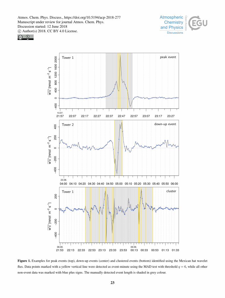
−400

040

080

012

0016

0020

00

13.07.21:57 22:07 22:17 22:27 22:37 22:47 22:57 23:07 23:17 23:27

w′c

′[nm

olm

−2s−1

]

Tower 1 peak event−4

00−2

000

200

400

23.08.

04:00 04:10 04:20 04:30 04:40 04:50 05:00 05:10 05:20 05:30 05:40 05:50 06:00

w′c

′[nm

olm

−2s−1

]

Tower 2 down-up event

200

−400

−200

0

08.09.21:53 22:13 22:33 22:53 23:13 23:33 23:53

09.09.00:13 00:33 00:53 01:13 01:33

w′c

′[nm

olm

−2s−1

]

Tower 1 cluster

Figure 1. Examples for peak events (top), down-up events (center) and clustered events (bottom) identified using the Mexican hat wavelet

flux. Data points marked with a yellow vertical line were detected as event-minute using the MAD test with threshold q = 6, while all other

non-event data was marked with blue plus signs. The manually detected event length is shaded in grey colour.

23


d.1Hz$T_begin

−0.2

0.0

0.2

0.4

[ms−1

]w

u*

d.1Hz$T_begin

2200

2600

3000

3400

c[n

mol

mol

−1]

d.1Hz$T_begin

0.5

1.5

2.5

U [m

s−1]

d.cur$T_begin[s]

9092

9496

9810

0[%

]R

(4.6

m)R

(2.0

m)

u_dir_time[s] + 5 * 60

φK

↓[W

m−2

]−1

.0−0

.50.

00.

51.

0

d.cur$T_begin[s]

2426

2830

3234

I↑+

I↓[W

m−2

]

p [h

Pa]

1010

.62

1010

.68

1010

.74

d cur$T begin[s]16

.017

.018

.019

.0 [°C]

T (4

.6m

)T (2

.0m

)02.08.23:00 23:10 23:20 23:30 23:40 23:50

03.08.00:00 00:10 00:20 00:30 00:40 00:50 01:00

N NE E SE S SW W NW337.5 ° 22.5 ° 67.5 ° 112.5 ° 157.5 ° 202.5 ° 247.5 ° 292.5 ° 337.5 °

Figure 2. Meteorological conditions observed at tower 1 during the case study event of August 02./03., 2014. Wind velocity U , vertical wind

speed wand CH4 mixing ratio c as well as wind direction φ are shown in a time resolution of 20 Hz. The friction velocity u∗ was averaged to

30 min, while all other data were averaged to 10 min: relative humidity R and air temperature T (both in each 2.0 and 4.5 m above ground)

as well as the longwave radiation balance I ↓+I ↑, the shortwave downwelling radiation K ↓ and air pressure p. The bottom panel shows a

legend for φ.

24


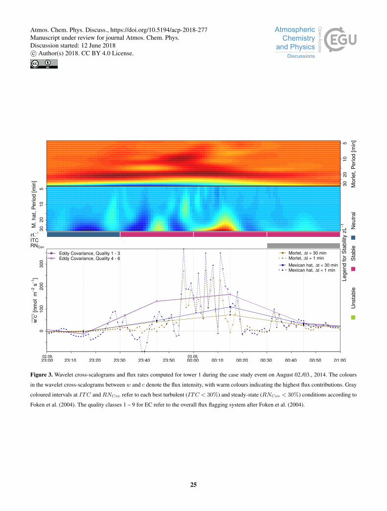
300

Time

3020

105

Mor

let,

Perio

d [m

in]

M. h

at, P

erio

d [m

in]

3020

105

Stab

leN

eutra

l

d.cur$T_begin

zL−1

ITCRNCov

Lege

nd fo

r Sta

bilit

y zL

−1

100

200

●

●

●

Eddy Covariance, Quality 1 - 3Eddy Covariance, Quality 4 - 6

Mexican hat, Δt = 30 min

Morlet, Δt = 30 min


Δt = 1 min

02.08.23:00 23:10 23:20 23:30 23:40 23:50

03.08.00:00 00:10 00:20 00:30 00:40 00:50 01:00

Morlet,

Uns

tabl

e

0w

′c′[nm

olm

−2s−1

]

Figure 3. Wavelet cross-scalograms and flux rates computed for tower 1 during the case study event on August 02./03., 2014. The colours

in the wavelet cross-scalograms between w and c denote the flux intensity, with warm colours indicating the highest flux contributions. Gray

coloured intervals at ITC and RNCov refer to each best turbulent (ITC < 30%) and steady-state (RNCov < 30%) conditions according to

Foken et al. (2004). The quality classes 1 – 9 for EC refer to the overall flux flagging system after Foken et al. (2004).

25


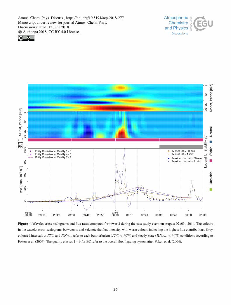
Time

d.cur$T_begin

200

400

600

●●

M. h

at, P

erio

d [m

in]

3020

105

3020

105

Mor

let,

Perio

d [m

in]

zL−1

ITCRNCov

02.08.23:00 23:10 23:20 23:30 23:40 23:50

03.08.00:00 00:10 00:20 00:30 00:40 00:50 01:00

Stab

leN

eutra

lLe

gend

for S

tabi

lity

zL−1

Uns

tabl

e

Eddy Covariance, Quality 1 - 3Eddy Covariance, Quality 4 - 6Eddy Covariance, Quality 7 - 8

0


Morlet, Δt = 30 min


Δt = 1 minMorlet,

w′c

′[nm

olm

−2s−1

]80

0

Figure 4. Wavelet cross-scalograms and flux rates computed for tower 2 during the case study event on August 02./03., 2014. The colours

in the wavelet cross-scalograms between w and c denote the flux intensity, with warm colours indicating the highest flux contributions. Gray

coloured intervals at ITC and RNCov refer to each best turbulent (ITC < 30%) and steady-state (RNCov < 30%) conditions according to

Foken et al. (2004). The quality classes 1 – 9 for EC refer to the overall flux flagging system after Foken et al. (2004).

26


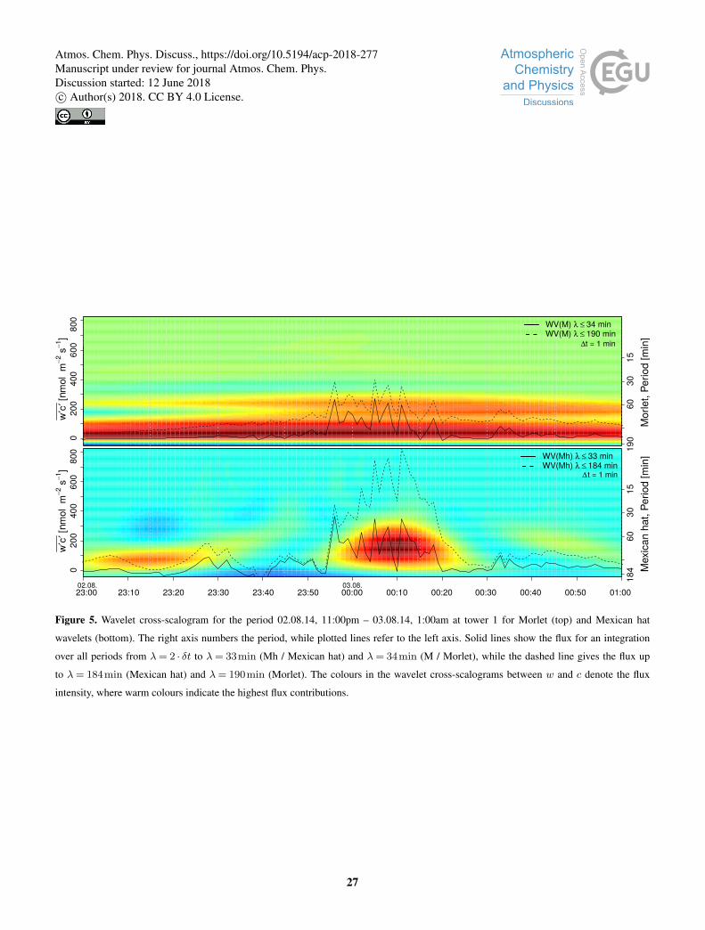
Time

190

6030

15M

orle

t, Pe

riod

[min

]

WV(M) λ ≤ 34 minWV(M) λ ≤ 190 min

Time

184

6030

15M

exic

an h

at, P

erio

d [m

in]WV(Mh) λ ≤ 33 min

WV(Mh) λ ≤ 184 min

02.08.23:00 23:10 23:20 23:30 23:40 23:50

03.08.00:00 00:10 00:20 00:30 00:40 00:50 01:00

020

040

060

0

Δt = 1 min

Δt = 1 min

w′c

′[nm

olm

−2s−1

]0

200

400

600

w′c

′[nm

olm

−2s−1

]80

080

0

Figure 5. Wavelet cross-scalogram for the period 02.08.14, 11:00pm – 03.08.14, 1:00am at tower 1 for Morlet (top) and Mexican hat

wavelets (bottom). The right axis numbers the period, while plotted lines refer to the left axis. Solid lines show the flux for an integration

over all periods from λ= 2 · δt to λ= 33min (Mh / Mexican hat) and λ= 34min (M / Morlet), while the dashed line gives the flux up

to λ= 184min (Mexican hat) and λ= 190min (Morlet). The colours in the wavelet cross-scalograms between w and c denote the flux

intensity, where warm colours indicate the highest flux contributions.

27


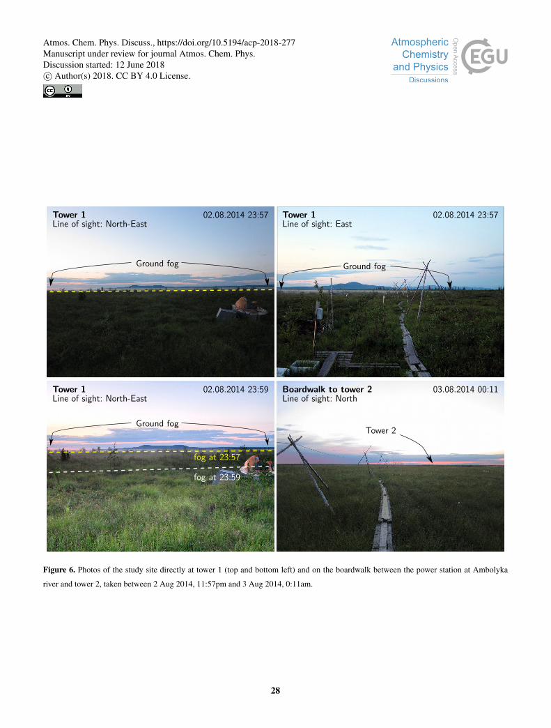
Tower 1 02.08.2014 23:57Line of sight: North-East

Ground fog

Tower 1 02.08.2014 23:57Line of sight: East

Ground fog

Tower 1 02.08.2014 23:59Line of sight: North-East

Ground fog

fog at 23:57

fog at 23:59

Boardwalk to tower 2 03.08.2014 00:11Line of sight: North

Tower 2

Figure 6. Photos of the study site directly at tower 1 (top and bottom left) and on the boardwalk between the power station at Ambolyka

river and tower 2, taken between 2 Aug 2014, 11:57pm and 3 Aug 2014, 0:11am.

28


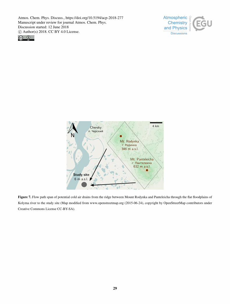
Study site

6 m a.s.l.

Cherskyп. Черский

Mt. Rodynkaг. Родинка

Mt. Panteleichaг. Пантелеиха632 m a.s.l.

346 m a.s.l.

4 km

Figure 7. Flow path span of potential cold air drains from the ridge between Mount Rodynka and Panteleicha through the flat floodplains of

Kolyma river to the study site (Map modified from www.openstreetmap.org (2015-06-24), copyright by OpenStreetMap contributors under

Creative Commons License CC-BY-SA).

29


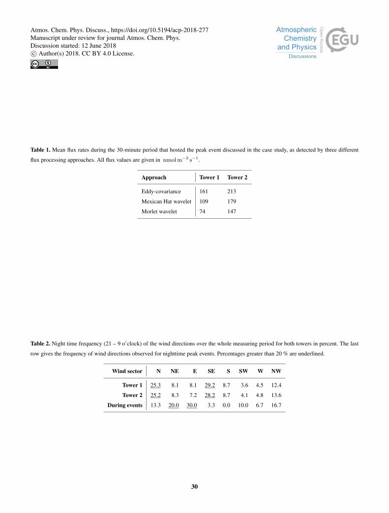
Table 1. Mean flux rates during the 30-minute period that hosted the peak event discussed in the case study, as detected by three different

flux processing approaches. All flux values are given in nmolm−2 s−1.

Approach Tower 1 Tower 2

Eddy-covariance 161 213

Mexican Hat wavelet 109 179

Morlet wavelet 74 147

Table 2. Night time frequency (21 – 9 o’clock) of the wind directions over the whole measuring period for both towers in percent. The last

row gives the frequency of wind directions observed for nighttime peak events. Percentages greater than 20 % are underlined.

Wind sector N NE E SE S SW W NW

Tower 1 25.3 8.1 8.1 29.2 8.7 3.6 4.5 12.4

Tower 2 25.2 8.3 7.2 28.2 8.7 4.1 4.8 13.6

During events 13.3 20.0 30.0 3.3 0.0 10.0 6.7 16.7

30


characterisation of short-term extreme methane uxes

Documents