Character Physics and Animation in Full Auto

David WuPseudo Interactive

Introduction

Physical simulation of characters is an important problem in games.

In this lecture, the Framework for character simulation and animation that PI is developing will be presented.

Introduction (cont)

This framework is part of the latest incarnation of our physics engine, and is the basis for a game in development.

This means that the framework needs to actually work.

Goal

The primary goal of this presentation is to describe a collection of algorithms that can be used to solve the dynamic equations of characters, incorporate animation data into the solutions and integrate the results forward in time.

Goal

The main algorithms are:The Structurally Recursive

methods for inverse dynamicsImplicit Euler integrationMathematical Optimization

Goal (cont)

By the end of the lecture you should have an intuitive understanding of how the structurally recursive methods work to solve for the dynamics of a character and how implicit Euler can use the results to evolve the system dynamics through time.

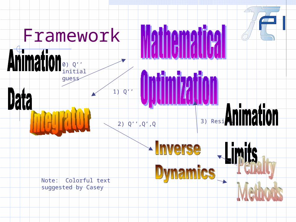
Framework

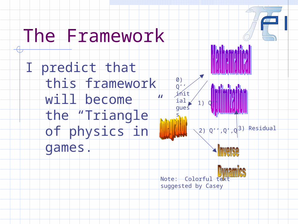
1) Q’’

3) Residual

0) Q’’ initial guess

2) Q’’,Q’,Q

Note: Colorful text suggested by Casey

Framework

1) Q’’

3) Residual

0) Q’’ initial guess

2) Q’’,Q’,Q

Note: Colorful text suggested by Casey

Goal (continued)

The secondary goal of this presentation is to get myself a free pass to GameTech.

The Framework

Physics in games is similar to where 3d rendering was in the early ‘90s.

There are many different approaches to solving the problem.

There is no commonly accepted standard.I.e. no “Triangle”.

The Framework

I predict that this framework will become the “Triangle” of physics in games.

1) Q’’

3) Residual

0) Q’’ initial guess

2) Q’’,Q’,Q

Note: Colorful text suggested by Casey

The Framework

VersatileRobustStable performanceSimple APIExplicit Control of DOF

• useful for Animation

1) Q’’

3) Residual

0) Q’’ initial guess

2) Q’’,Q’,Q

Note: Colorful text suggested by Casey

Disclaimer

I am often wrong.

Physical Entities

All Physical entities are made up of “Frames”A Frame has Degrees of Freedom (DOF) and can perform spatial transformation from local space to global space.For this lecture we will only consider rigid bodies, although the algorithms that are described can support arbitrary DOF, including, for example, finite element nodes.

Character Example

Each set of arrows is a FrameAll frames are related to their parent using relative coordinatesEach frame is Rigid from a physics stand point (although the mesh uses skinning) Closed loops require constraints

Character Example

DOF Breakdown: Root (chest) 6 Pelvis 3 Thighs 3 (*2) Knees 1 (*2) Feet 3 (*2) Shoulders 3 (*2) Elbows 1 (*2) Wrists 3 (*2)

Total: 14 Frames, 37 DOF

Physics of Characters

There are a number of ways to derive the dynamics of characters. The method that I will describe is based on the structurally recursive methods. There are a number related techniques that all use the same concepts:

Featherstone's method Articulated Rigid Body Method Recursive Newton-Euler Equations Composite Rigid Body Method Etc.

Physics of Characters

An intuitive understand of how the method works is important.As such, the presentation will start from first principles and emphasize verbal descriptions.Part of the motivation behind this is the difficulty of writing equations or code in PowerPoint.

First PrinciplesConsider the momentum of a single rigid body at time t0:

Mt0*Vt0

M is a sparse 6x6 Matrix Mass Moments of Inertia

V is a 6d vector 3d Velocity at Center of

mass 3d Angular velocity This is often called the

“Spatial Velocity Vector”

M

vw

Some notes on the M matrix

Since M is in global coordinates, it is generally dependant on the rigid bodies orientation in space. This is what gives rise to the coriolis terms

If V was chosen to be at a point other than the center of mass, M would be less sparse and it would represent centrifugal effects.

Using the momentum equations we can safely ignore these effects - they are handled implicitly. I.e. when a valid solution is found, derivatives

of M will have contributed to the solution.

DynamicsConservation of momentum provides the

following constraint: Mt1*Vt1 = Mt0*Vt0 + integral(F,t0,t1)

F are external forces and torques

By the definition of velocity we have: Qt1 = Qt0 + integral(V,t0,t1)

Q is position and orientation These are the main equations that we

need to solve to ensure that the simulation is physically accurate.

How to solve?

Everyone’s favorite straw man…

Forward Euler

In order to approximate integral(F,t0,t1) we could compute F at t0 and then multiply it by (t1-t0).

Mt1*Vt1 = Mt0*Vt0 + Ft0*dt This is convenient because we know

the state of the system at t0, so we can just compute forces directly.

The approximation is that the forces at t0 are constant throughout the time step, which is pretty accurate if t1-t0 is very small.

Forward Euler

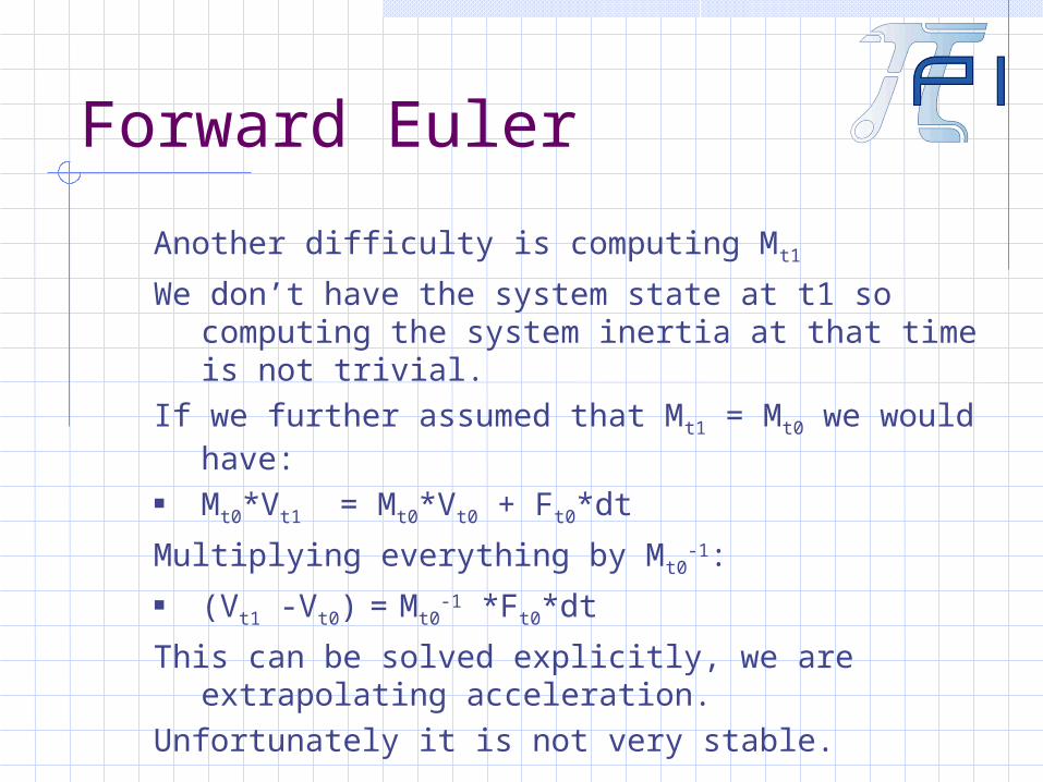
Another difficulty is computing Mt1

We don’t have the system state at t1 so computing the system inertia at that time is not trivial.

If we further assumed that Mt1 = Mt0 we would have:

Mt0*Vt1 = Mt0*Vt0 + Ft0*dt

Multiplying everything by Mt0-1:

(Vt1 -Vt0) = Mt0-1 *Ft0*dt

This can be solved explicitly, we are extrapolating acceleration.

Unfortunately it is not very stable.

Implicit Euler

With Forward Euler, we replaced all Integral(X,t0,t1)’s with Xt0*(t1-t0)

Assuming that we can ignore the difficulties of computing quantities at future points in time, we could instead replace Integral(X,t0,t1) with Xt1*(t1-t0)

This is implicit Euler, which is unconditionally stable for stable systems.

Implicit Euler

A simple example is a stiff spring

Ft0

Ft1

Vt0

Vt1

There is negative feedback for conservative potentials

Implicit Euler

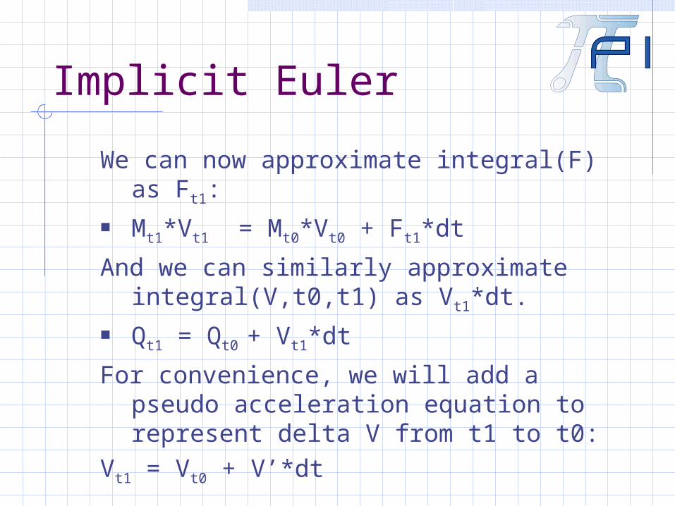
We can now approximate integral(F) as Ft1:

Mt1*Vt1 = Mt0*Vt0 + Ft1*dt

And we can similarly approximate integral(V,t0,t1) as Vt1*dt.

Qt1 = Qt0 + Vt1*dt

For convenience, we will add a pseudo acceleration equation to represent delta V from t1 to t0:

Vt1 = Vt0 + V’*dt

Nonlinear Equations

The implicit equations are difficult to solve because we need values at future points in time.

Another way of saying this is that we have unknowns all over the place, and some of the relationships are nonlinear.

Nonlinear Equations

As it turns out, these equations can be transformed into a convex optimization problem.

The function that we are minimizing is related to the systems kinetic and potential energy:

E=(Mt1*Vt1 - Mt0*Vt0 - Ft1*dt)*Vt1

The unknowns are the accelerationsThe convex constraints are the physical

constraints

Convex Optimization

As it turns out, these equations can be transformed into a convex optimization problem.

The function that we are minimizing is related to the systems kinetic and potential energy (the Lagrangian):

E=(Mt1*Vt1 - Mt0*Vt0 - Ft1*dt)*V’

The unknowns are the accelerations (V’)The convex constraints are the physical

constraints

Minimizing Energy

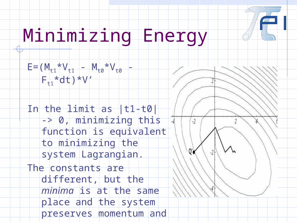
E=(Mt1*Vt1 - Mt0*Vt0 - Ft1*dt)*V’

In the limit as |t1-t0| -> 0, minimizing this function is equivalent to minimizing the system Lagrangian.

The constants are different, but the minima is at the same place and the system preserves momentum and energy.

Interior point methods

E=(Mt1*Vt1 - Mt0*Vt0 - Ft1*dt)*V’

One way to solve convex optimization problems is piecewise quadratic programming, another is the interior point method which is what we will use.

The interior point methods transform the constraints into penalty functions and then minimizes unconstrained nonlinear equations.

Penalty Methods

Penalty methods are intuitive - game developers have been using them for years, even developers who don’t know what they are.

The spring analogy provides a metaphor and API that is easy to use and understand.

You don’t have to worry too much about overconstrained systems, which are very difficult to avoid in games.

Nonlinear Equations

If we know what the acceleration is, we can step the system forward in time to compute Vt1, Mt1.

With this updated state we can compute Ft1.

We can then compute the Residual: R = Mt1*Vt1 - Mt0*Vt0 - Ft1*dt To see if the acceleration was physically correct.

Ft1

Vt1Vt0

step

Mathematical Optimization

There is a good management analogy here:

Rather than trying to find a solution, we can let someone else try out solutions and just let them know how wrong they are.

This is essentially the interface to mathematical optimizers

i.e. Conjugate Gradient Method, Newton's method, Gauss Seidel iterations

Minimizing Residual

For a given acceleration we compute

R = Mt1*Vt1 - Mt0*Vt0 - Ft1*dt.

R is how wrong the acceleration is.- If R is 0, the solution is correct.- In practice we don’t need exact 0’s, if we sufficiently minimize R the answer is good enough.

Optimizer API

The mathematical optimizer will use the residual to guide a search. The search tests a series of accelerations and eventually converges on the optimal solution.

Q’’ Residual

HessianNewton’s Method

minimizes nonlinear equations by approximating them as a piecewise quadratic function.

The Hessian is the matrix that represents the quadratic coefficients:

q*H*qt + qt*b + c = 0

Hessian

The Hessian of these equations turns out to be:

System inertia with respect to the DOF

+ a low pass filter due to implicit Euler integration

+ a filter due to constraints and penalty methods

Hessian

Intuitively the equation that the optimizer solves is similar to

F = MAM is the Hessian.

Constraints add “infite inertia”

Stiff springs make the system heavier w.r.t. their direction of action

Hessian

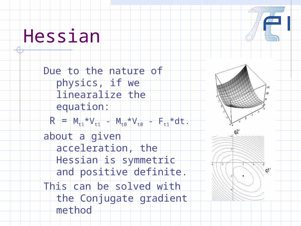
Due to the nature of physics, if we linearalize the equation:

R = Mt1*Vt1 - Mt0*Vt0 - Ft1*dt.

about a given acceleration, the Hessian is symmetric and positive definite.

This can be solved with the Conjugate gradient method

Hessian

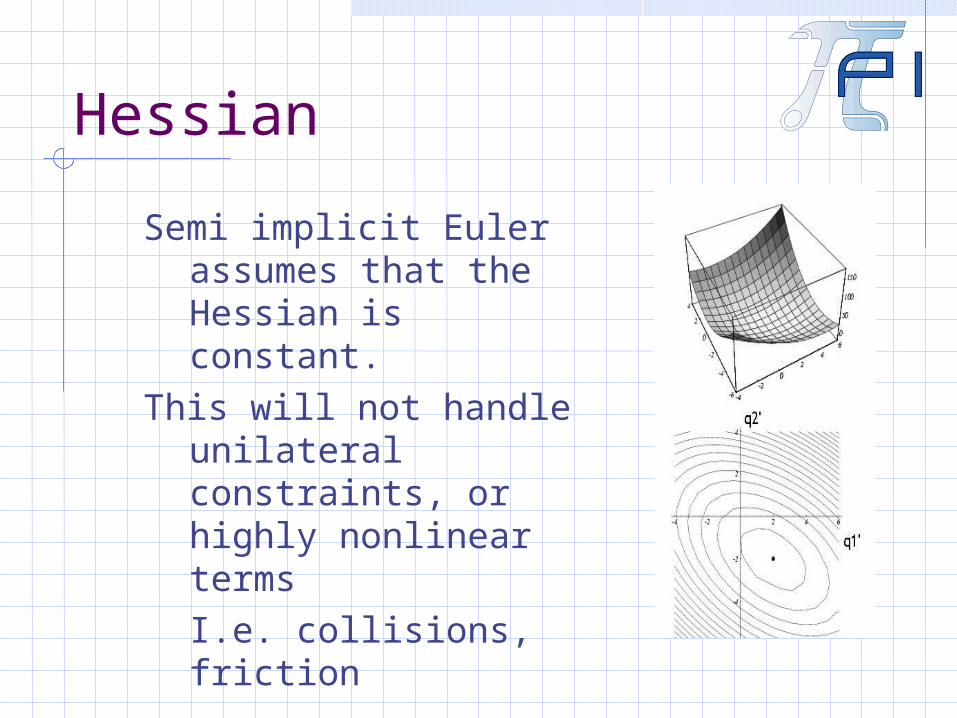
Semi implicit Euler assumes that the Hessian is constant.

This will not handle unilateral constraints, or highly nonlinear termsI.e. collisions, friction

Truncated Newton

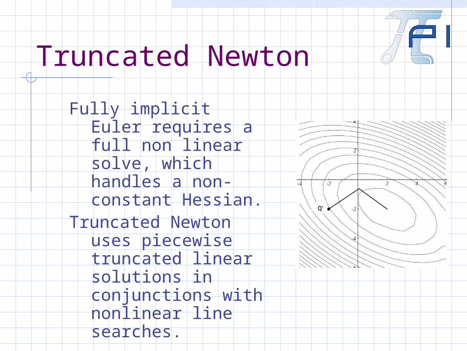
Fully implicit Euler requires a full non linear solve, which handles a non-constant Hessian.

Truncated Newton uses piecewise truncated linear solutions in conjunctions with nonlinear line searches.

Truncated Newton

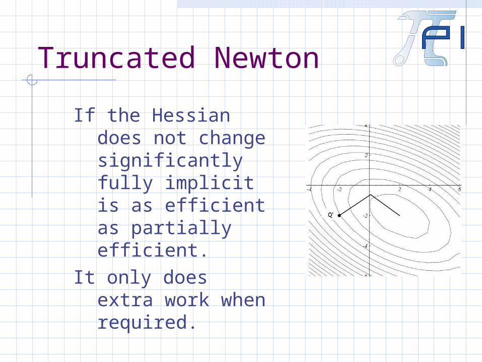
If the Hessian does not change significantly fully implicit is as efficient as partially efficient.

It only does extra work when required.

Simulation

In order to simulate the rigid body we: Guess at what the acceleration is, and give this

to the optimizer. The optimizer will feed us a number of guesses. For each guess we:

Step the system forward with the kinematic equations:

Vt1 = Vt0 + V’*dt Qt1 = Qt0 + Vt1*dt

Compute Ft1

Compute Mt1*Vt1

Compute the residual: R=Mt1*Vt1 - Mt0*Vt0 - Ft1*dt

Feed the residual back to the optimizer.

Simulation

In the case of unconstrained rigid bodies, the Hessian is Diagonally dominant, Conjugate gradient can solve these systems to a reasonable error in one step.

Inverse Dynamics

Computing Mt1*Vt1 - Mt0*Vt0 is similar to Inverse Dynamics, but in this case we are dealing with a finite change in time and velocity rather than an infinitesimal change. Inverse Dynamics computes forces

from accelerations. The problems are similar enough

that we can use similar techniques

Inverse Dynamics

Inverse dynamics is generally much easier than forward dynamics.A number of efficient methods for computing inverse dynamics have been developed by the robotics community.

A common application is to find a set of actuator torques required to achieve a set of joint accelerations

This technique can be used to efficiently determine physical quantities from animation data

Degrees of Freedom

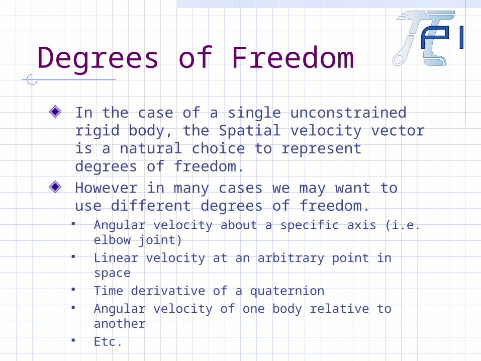
In the case of a single unconstrained rigid body, the Spatial velocity vector is a natural choice to represent degrees of freedom. However in many cases we may want to use different degrees of freedom.

Angular velocity about a specific axis (i.e. elbow joint)

Linear velocity at an arbitrary point in space Time derivative of a quaternion Angular velocity of one body relative to another Etc.

Jacobian

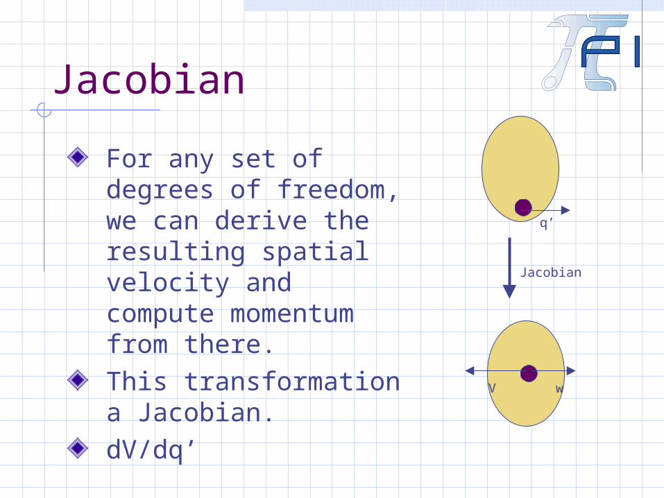
For any set of degrees of freedom, we can derive the resulting spatial velocity and compute momentum from there.This transformation a Jacobian.dV/dq’

q’

wV

Jacobian

Jacobian

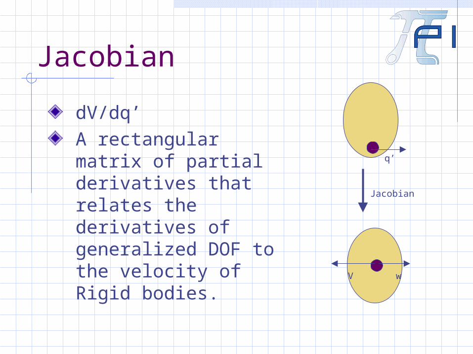
dV/dq’A rectangular matrix of partial derivatives that relates the derivatives of generalized DOF to the velocity of Rigid bodies.

q’

wV

Jacobian

Degrees of Freedom

Rigid bodies with their spatial velocities serve as a convenient Interface for various things such as constraints, potentials, contacts, computation of momentum etc.So most systems can only worry about rigid bodies and not deal with the fact that it might be a part of a character.

Attempting to interface at this level of abstraction is not recommended at social functions.

q’

wV

Jacobian

Degrees of Freedom

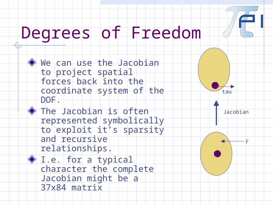
We can use the Jacobian to project spatial forces back into the coordinate system of the DOF.The Jacobian is often represented symbolically to exploit it’s sparsity and recursive relationships.I.e. for a typical character the complete Jacobian might be a 37x84 matrix

tau

Jacobian

F

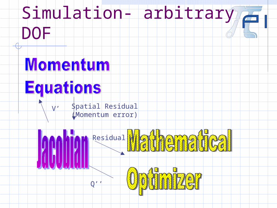
Simulation- arbitrary DOF

Q’’

Residual w.r.t. Q

V’ Spatial Residual(Momentum error)

Simulation- Hessian

Q’’

V’

A Hessian is the System inertia projected into DOF space + a low pass filter due to Implicit Euler

Simulation- arbitrary DOF

So in order to simulate any physical mechanism we can do the following:

Given the system state at t0, and an acceleration q’’.

Compute updated positions and velocities (q’,q) Compute spatial velocity (V), position and

orientation of the Rigid bodies Compute the Momentum of the rigid bodies Compute external forces Compute the residual R=Mt1*Vt1 - Mt0*Vt0 - Ft1*dt Project the residual back into DOF space for the

Mathematical Optimization system to deal with

vw

Constrained Rigid Body

Consider a rigid body constrained to rotate about an axis a.It has 1 degree of freedom (q, q’)The Jacobian relating q’ to V is the 1x6 matrix:

J = { Cross(a,r), a }t

V = J*q’M*V = M*J*q’So the residual in terms of q’’

projected onto q is:R=(M*J*(q’+q’’*dt) – Mt0*Vt0 - F) * Jt

a

r

F

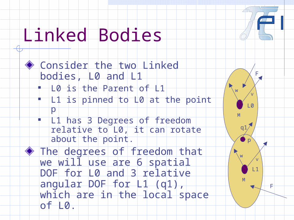
Linked Bodies

Consider the two Linked bodies, L0 and L1

L0 is the Parent of L1 L1 is pinned to L0 at the point p L1 has 3 Degrees of freedom

relative to L0, it can rotate about the point.

The degrees of freedom that we will use are 6 spatial DOF for L0 and 3 relative angular DOF for L1 (q1), which are in the local space of L0.

M

vw

M

vw

L0

L1

F

F

p

q1

Linked Bodies Kinematics

R0 is the vector from L0’s center of mass to the pivot pR1 is the vector from p to L1’s center of mass.A0 is the orientation of L0The angular velocity of L1 is:

Vl0.angular + A0*q1

The linear velocity of L1 is: Vl0.linear +

cross(Vl0.angular,r0) + cross(A0*q1,r1)

M

vw

M

vw

L0

L1

F

F

p

r0

r1

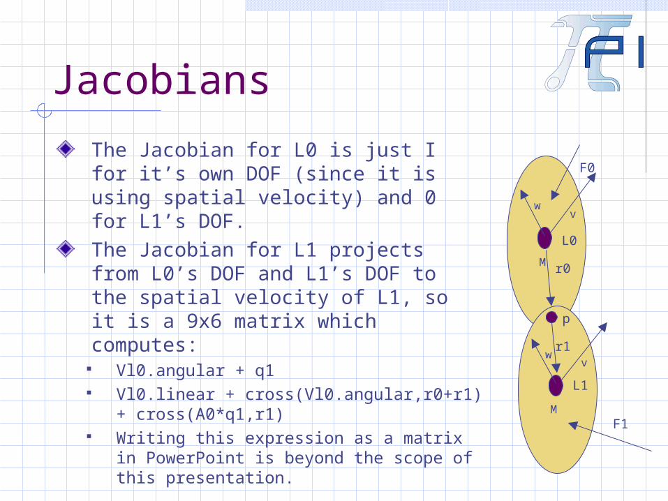
Jacobians

The Jacobian for L0 is just I for it’s own DOF (since it is using spatial velocity) and 0 for L1’s DOF.The Jacobian for L1 projects from L0’s DOF and L1’s DOF to the spatial velocity of L1, so it is a 9x6 matrix which computes:

Vl0.angular + q1 Vl0.linear + cross(Vl0.angular,r0+r1)

+ cross(A0*q1,r1) Writing this expression as a matrix in

PowerPoint is beyond the scope of this presentation.

M

vw

M

vw

L0

L1

F1

F0

p

r0

r1

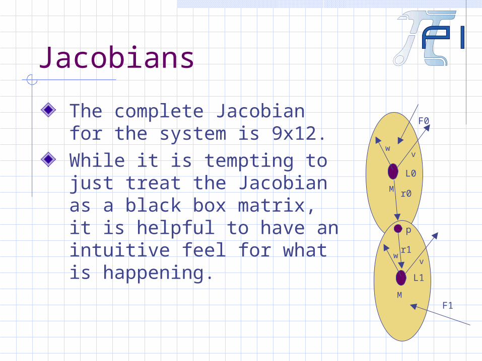
Jacobians

The complete Jacobian for the system is 9x12.While it is tempting to just treat the Jacobian as a black box matrix, it is helpful to have an intuitive feel for what is happening.

M

vw

M

vw

L0

L1

F1

F0

p

r0

r1

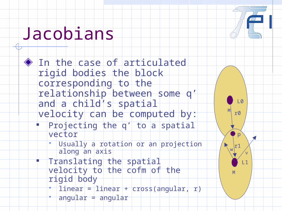
Jacobians

In the case of articulated rigid bodies the block corresponding to the relationship between some q’ and a child’s spatial velocity can be computed by:

Projecting the q’ to a spatial vector Usually a rotation or an projection

along an axis Translating the spatial velocity to

the cofm of the rigid body linear = linear + cross(angular, r) angular = angular

M

M

vw

L0

L1

p

r0

r1

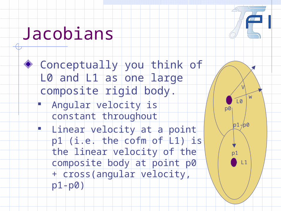
Jacobians

Conceptually you think of L0 and L1 as one large composite rigid body.

Angular velocity is constant throughout

Linear velocity at a point p1 (i.e. the cofm of L1) is the linear velocity of the composite body at point p0 + cross(angular velocity, p1-p0)

L0

L1

p0

p1

p1-p0

V

w

Jacobians

When projecting from spatial forces back into DOF the block corresponding to the relationship between the force on a body and a parent’s DOF can be computed by:

Translating the spatial force to pivot (or cofm) of the DOF Linear = linear angular = angular + cross(r,linear)

Projecting the spatial vector onto the DOF Usually a rotation or an projection

along an axis This is the Transpose of what we saw

on the last slide

M

M

L0

L1

F1

F0

p

r0

r1

Jacobians

Considering L0 and L1 as one large composite rigid body,

Linear Force is applied at any point results in a constant force throughout

Linear Force applied to point p1 creates an addition angular torque (moment) at p0 equal to cross(p1-p0, F)

L0

L1

p0

p1

p1-p0

F

Residual

Armed with the Jacobian, computing the residual is straight forward.

Spatial Momentum (M*V) is computed for each body

Spatial forces (F0,F1) are computed on each body as usual

The residual is computed for each body:

R=(Mt1*Vt1 – Mt0*Vt0 - F) The residuals are projected

onto the DOF using the Jacobian.

M

vw

M

vw

L0

L1

F1

F0

p

r0

r1

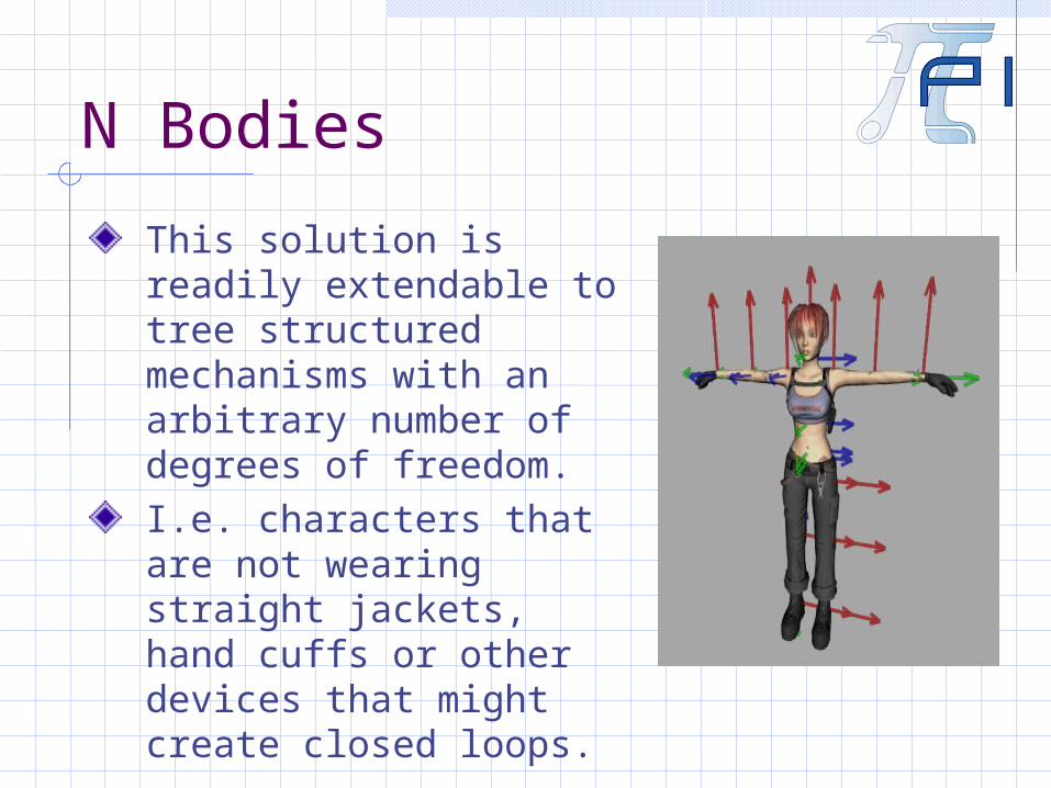
N Bodies

This solution is readily extendable to tree structured mechanisms with an arbitrary number of degrees of freedom. I.e. characters that are not wearing straight jackets, hand cuffs or other devices that might create closed loops.

N Bodies

Direct computation of the Jacobian requires O(n2) time and O(n2) space.We can use a recursive technique that processes direct child-parent relationships to compute the product of the Jacobian and a vector in O(n) time. These are called the Recursive Newton Euler equations.

N Bodies

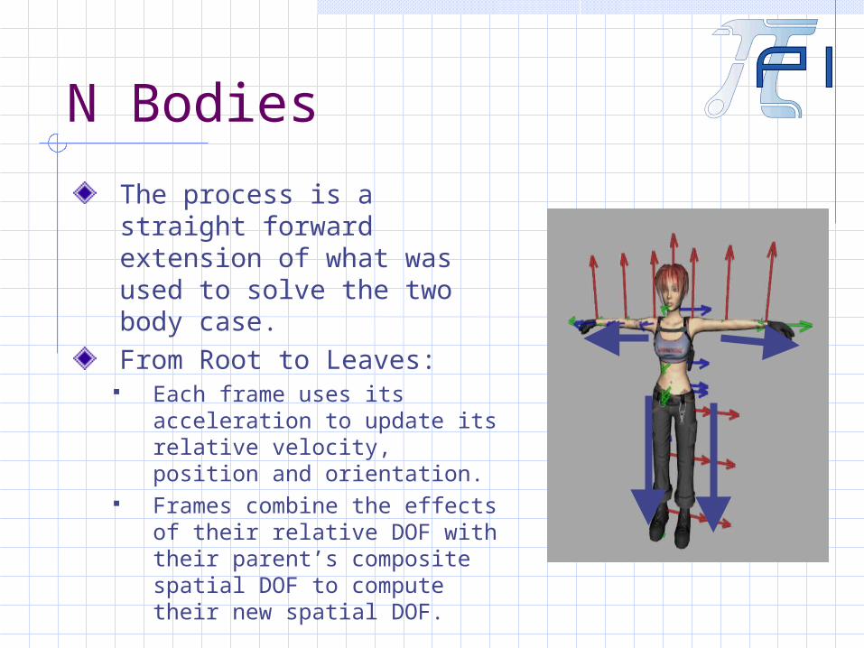
The process is a straight forward extension of what was used to solve the two body case.From Root to Leaves:

Each frame uses its acceleration to update its relative velocity, position and orientation.

Frames combine the effects of their relative DOF with their parent’s composite spatial DOF to compute their new spatial DOF.

N Bodies

Compute External Forces on all bodiesFrom Leaves to Root, for each frame:

Compute spatial momentum

Compute local residual Add the composite

residual of all children Project the residual onto

DOF

N Bodies

When a parent passes its composite velocity down to its children it is providing the results from O(n) grand parents.When each child passes its composite residual up to its parent it is providing the results of O(n) grandchildren.This is how the problem is reduced from O(n2) time to O(n) time.

Just another Jacobian

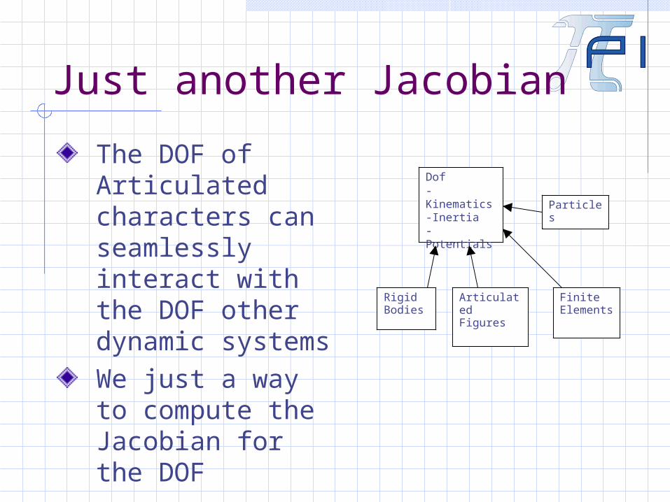
The DOF of Articulated characters can seamlessly interact with the DOF other dynamic systemsWe just a way to compute the Jacobian for the DOF

Dof-Kinematics-Inertia-Potentials

Particles

Rigid Bodies

Articulated Figures

Finite Elements

Just another Jacobian

Forward Dynamics

This technique can be extended to forward dynamics

I.e. the Articulated rigid body method

Unfortunately when you have constraints and closed loops (i.e. contacts) things rapidly increase above O(n) time.Forward dynamics can be used to precondition the system for the optimizer.

Kinematics

A convenient property of this solution is that specific DOF can be set to kinematic with very few changes:The accelerations of the kinematic DOF are not given to the mathematical optimizer, instead they are assumed to be constants.When the residual is computed for Kinematic DOF, it is not given back to the optimizer.

Kinematics

Kinematic DOF reduce the number of unknowns that the optimizer has to solve for. This improves convergence and speeds up the solution.A technique that we use to LOD simulation is to “Bake” certain DOF when stress is high.

I.e. wrists and ankles are dynamic ¼ of the time, and kinematic with q’’ = -q’*kd the rest of the time.

Animation

Animation data can be applied to dynamic characters as follows:

All DOF are set to kinematic with q’’ derived from the animation

The DOF space residuals are compared with some threshold representing the maximum force/torque that the characters muscles can apply.

If the residual is <= this limit, everything is fine.

If the residual is >= this limit, the limit is applied and the DOF is switched to dynamic.

Animation

This provides a very efficient mechanism to combine animations with physics.When all residuals are within limits, the costs are very similar to that of straight animation playback.

I.e. there are 0 unknown DOF, which is easy to solve for.

Animation

Switching back and forth between dynamic and kinematic is perfectly legal within the context of convex optimization, provided that the actuator force applied when the DOF are dynamic are >= than the highest residual seen when they were kinematic.

Animation

Rather than removing the kinematic DOF from the optimizer, you can just set the residual’s to 0 and the optimizer will not change the DOF. This is equivalent to applying a force that is exactly equal and opposite to the residual at the DOF, which is what an ideal actuator would do.The function is min(torque limit,residual) This would break a semi implicit integrator.

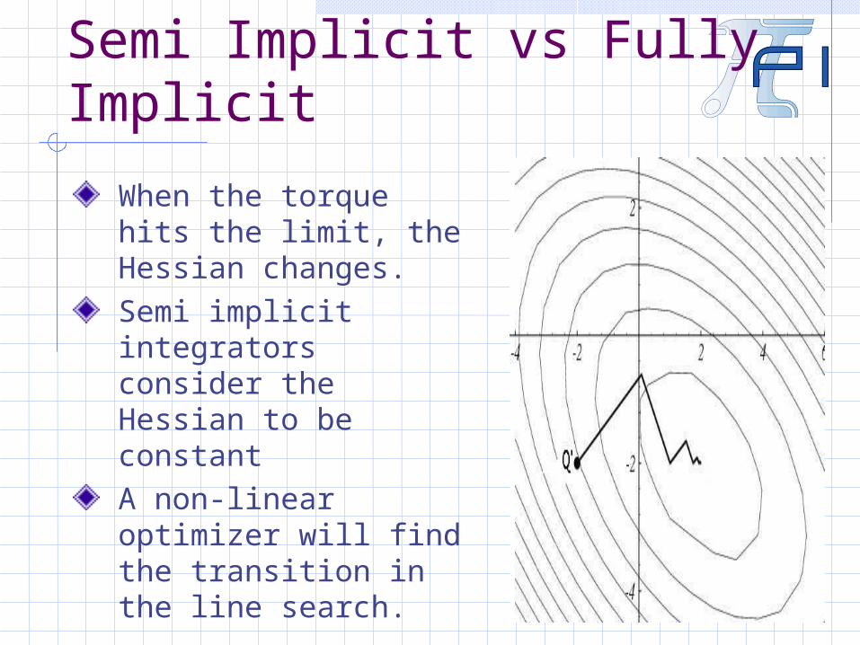
Semi Implicit vs Fully Implicit

When the torque hits the limit, the Hessian changes. Semi implicit integrators consider the Hessian to be constantA non-linear optimizer will find the transition in the line search.

Limitations

Finding the wrong root. A non-linear system can have multiple local

minima. The worst offenders are rotational DOF with

very little inertia subject to large external forces I.e. foot on ground supporting body Luckily the animation actuator increases the effective

inertia of the DOF It helps to give characters strong calves.

In order for this to be a problem at a 60hz simulation rate, you have to encounter angular accelerations that are ~ 3600 radians/second2

Limitations

First order accurate For us the error is acceptable when

simulating at >= 60hz.

Adds damping

Summary

Lots of stuff was covered.

Questions