BIOL2300 Biostatistics

Chapters 2, 3 Descriptive Statistics (histograms, box plots, avg, stdev)

From Cartoon Guide to Statistics, Gonick & Smith

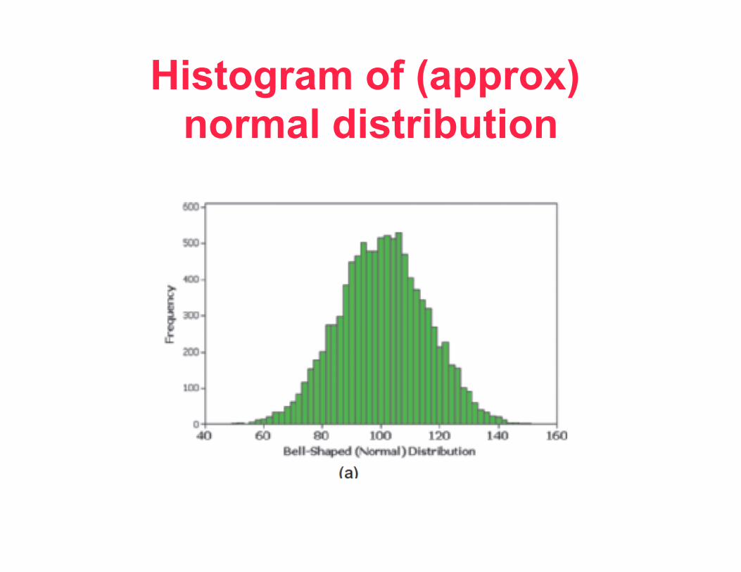
Histogram of (approx) normal distribution

Histogram of (approx) uniform distribution

Histogram of right-skewed distribution

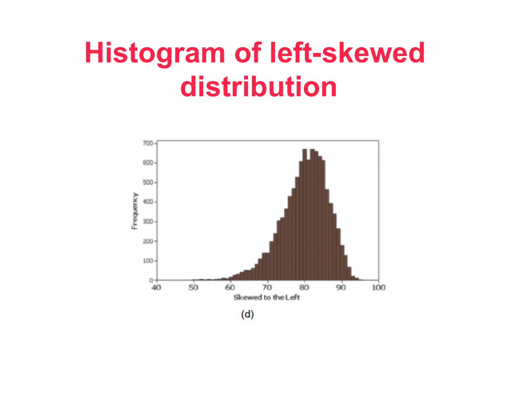
Histogram of left-skewed distribution

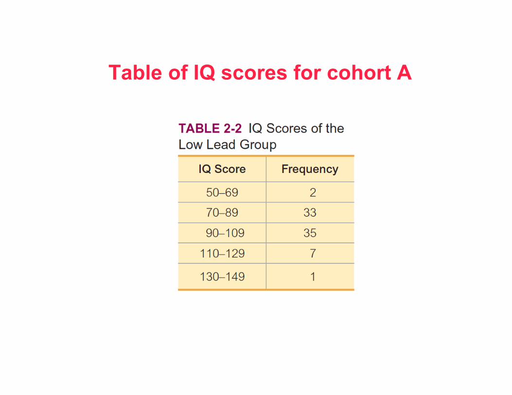
Table of IQ scores for cohort A

Definitions needed to construct a histogram

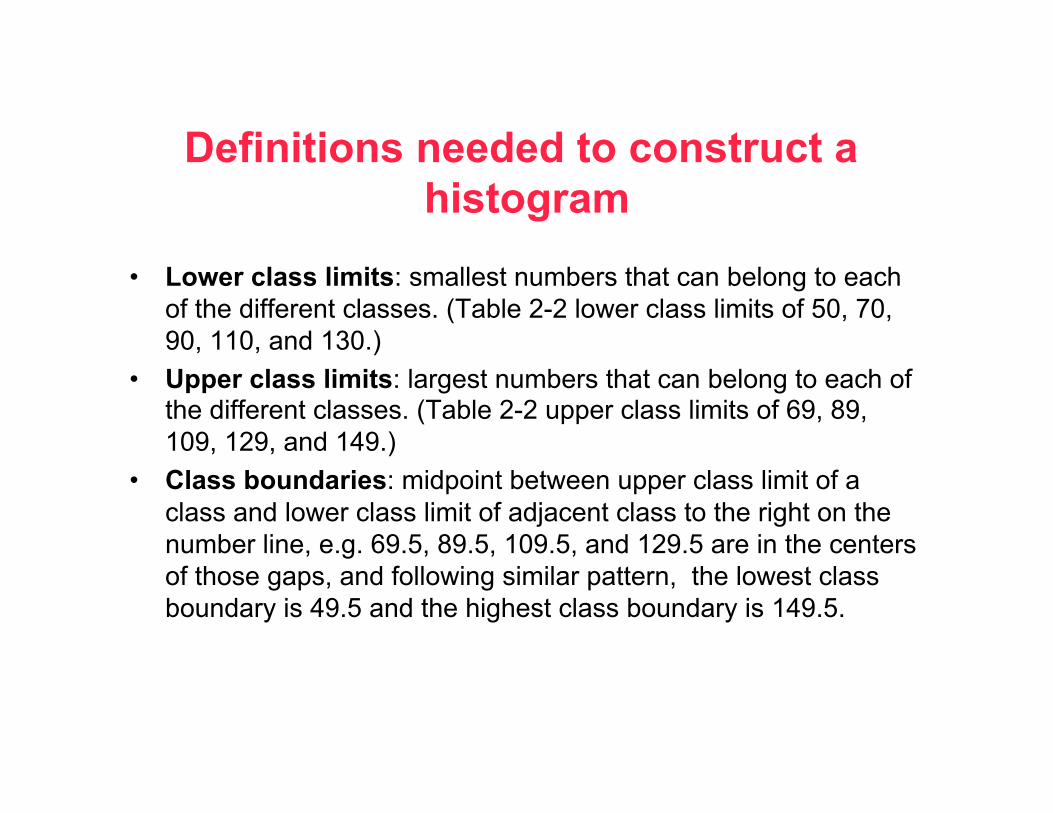
•  Lower class limits: smallest numbers that can belong to each of the different classes. (Table 2-2 lower class limits of 50, 70, 90, 110, and 130.)

•  Upper class limits: largest numbers that can belong to each of the different classes. (Table 2-2 upper class limits of 69, 89, 109, 129, and 149.)

•  Class boundaries: midpoint between upper class limit of a class and lower class limit of adjacent class to the right on the number line, e.g. 69.5, 89.5, 109.5, and 129.5 are in the centers of those gaps, and following similar pattern, the lowest class boundary is 49.5 and the highest class boundary is 149.5.

Definitions needed to construct a histogram

•  Class midpoints: values in the middle of the classes. Table 2-2 has class midpoints of 59.5, 79.5, 99.5, 119.5, and 139.5. Each class midpoint is computedby adding the lower class limit to the upper class limit and dividing the sum by 2.

•  Class width: difference between two consecutive lower class limits (or two consecutive lower class boundaries) in a frequency distribution. Table 2-2 uses a class width of 20. (The first two lower class boundaries are 50 and 70, and their difference is 20.)

Finding class boundaries

Exposure to smoking in environment

Smokers: relative frequency histogram

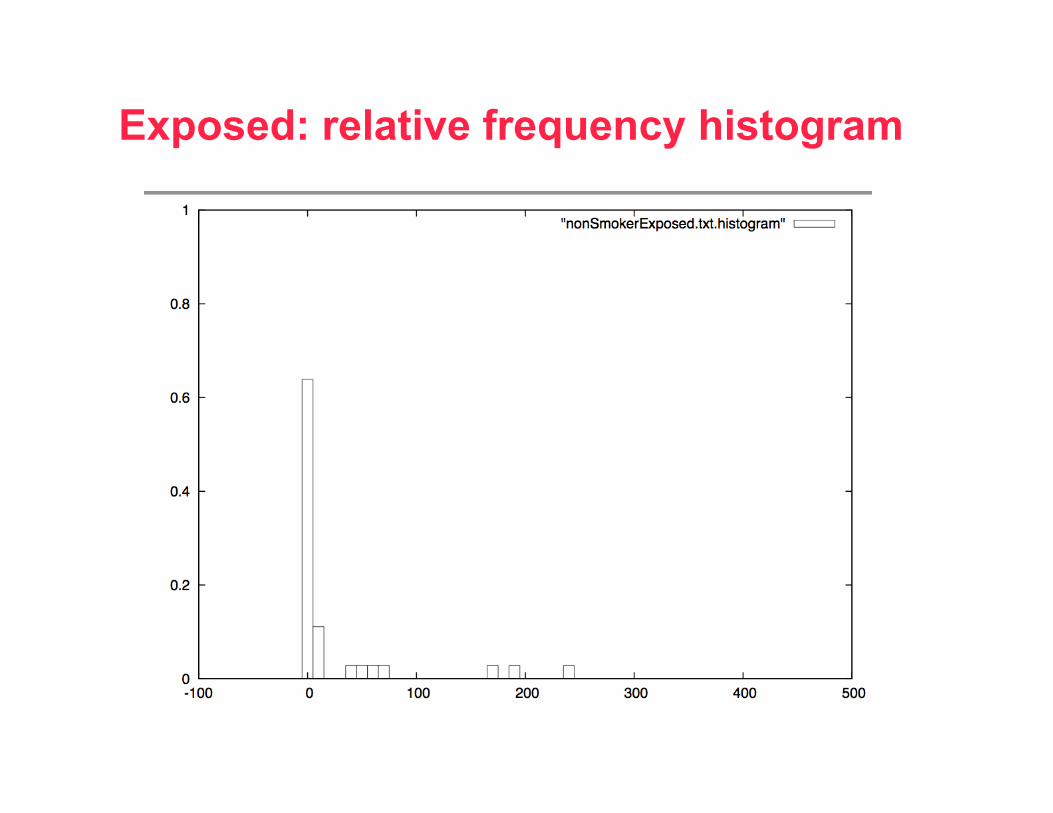
Exposed: relative frequency histogram

Nonexposed: relative frequency histogram

Exposed/nonexposed

Interpretation of data

•  It’s clear that nonsmokers, who are exposed to second-hand smoke, have higher cotinine traces (cotinine is a metabolic byproduct of nicotine).

•  Is this difference statistically significant? •  Is the significance sufficiently important to

warn the public about the danger of environmental smoke exposure, given the possibility of law suits by the tobacco industry?

Interpretation of data

•  It’s clear that nonsmokers, who are exposed to second-hand smoke, have higher cotinine traces (cotinine is a metabolic byproduct of nicotine).

•  Is this difference statistically significant? •  Is the significance sufficiently important to

warn the public about the danger of environmental smoke exposure, given the possibility of law suits by the tobacco industry?

Mean, standard deviation, min, max

•  SMOKER – Mean:181.526316 StDev:114.092469

Max:491 Min:1 •  EXPOSED

– Mean:56.527778 StDev:132.065532 Max:551 Min:0

•  Nonexposed – Mean:18.138889 StDev:64.840468 Max:

309 Min:0

Roundoff rule •  If n-place accuracy in data, then

round off to n+1-place accuracy •  Previous results should be

presented with 1-place accuracy •  WARNING: ONLY at the very end

when summarizing data (not curing calculations!!!)

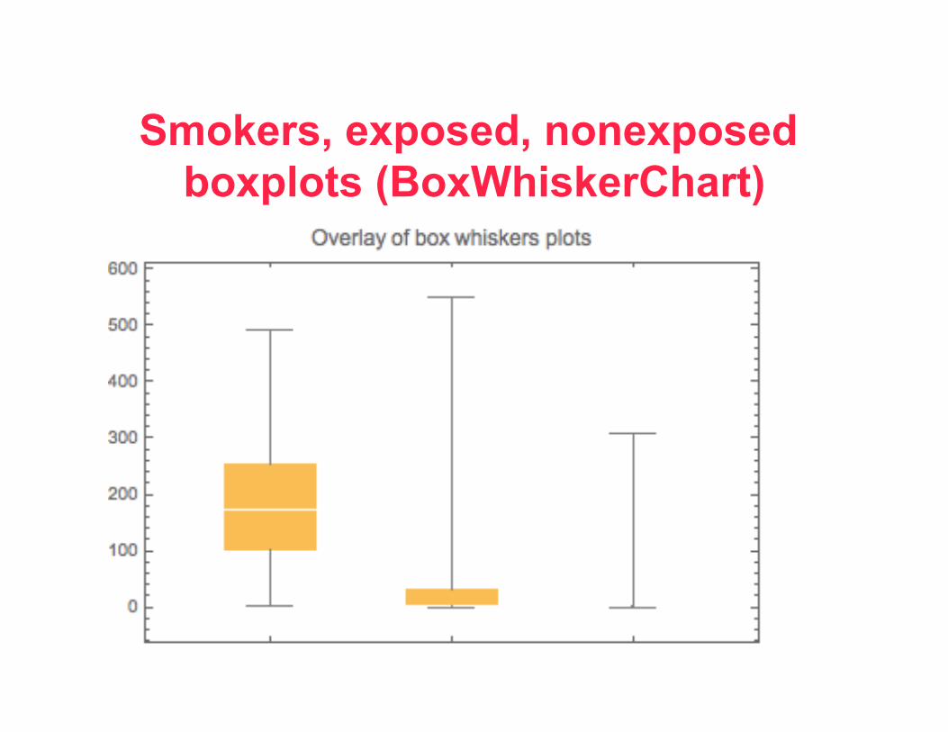
Smokers, exposed, nonexposed boxplots (BoxWhiskerChart)

Definitions 0-59 F 60-69 D 70-79 C 80-89 B 90-100 A

•  lower class limits: 0,60,70,80,90 •  upper class limits: 59,69,79,89,100 •  class boundaries: midpoints between

successive upper and lower class limits, eg –  0.5, 59.5, 69.5, 79.5, 89.5,100.5

•  class width: difference of two successive lower class boundaries (or of two successive upper class boundaries) -- class widths are 60,10,10,10,11

•  class midpoints: (max+min)/2 where min and max are respectively minimum and maximum of class, eg (59+0)/2, (69+60)/2, etc. (Reminder: (a+b)/2 = a +(b-a)/2.)

•  frequency distribution: function that counts the number of data items lying in an interval, for a given collection of intervals. Generally the interval [min,max] is divided into equal size subintervals, whose left endpoints are min+i(max-min)/N for i=0,1,...,N-1. There are N bins (buckets), where the i-th bin consists of all data values lying in the i-th subinterval, i.e. the half-open interval

[min+(i-1)(max-min)/N,min+i(max-min)/N)

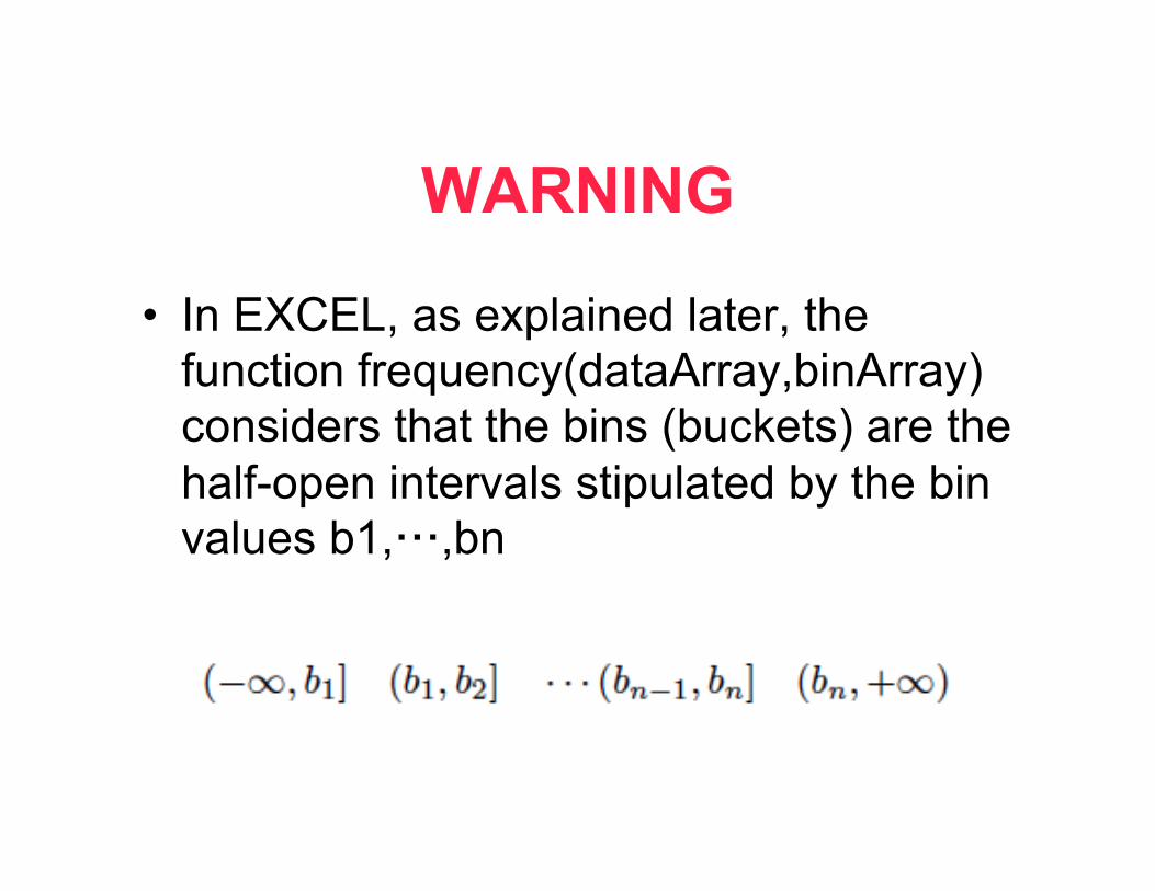
WARNING

•  In EXCEL, as explained later, the function frequency(dataArray,binArray) considers that the bins (buckets) are the half-open intervals stipulated by the bin values b1,…,bn

•  frequency = absolute frequency = count •  relative frequency = count/total number of objects

rel freq = class frequency/sum of all freq •  relative frequency distribution •  cumulative frequency distribution: if

f: {0,1,...,N-1} --> non-negative integers is a frequency distribution, then the cumulative frequency is defined by F {0,1,...,N-1} à non-negative integers where F(0)=f(0) F(i) = f(0)+...+f(i)

TRICK: inverting the cumulative relative frequency distribution to simulate any discrete distribution, such as exon lengths used in GenScan software (human gene finder)

•  histogram: bar graph representing frequency distribution

•  frequency polygon: line segments connecting points where xi is midpoint of i-th class and yi is frequency of i-th class

•  ogive: line graph depicting cumulative frequency

•  dotplot: place a dot on the number line for data values

•  stem and leaf plot: stem is integer portion, leaves form a list of the decimal portions

Images http://www.purplemath.com/modules/stemleaf.htm

•  Pareto chart: a variant of histogram where subintervals are sorted in decreasing order of frequency values

•  scatter plot: plot of (x,y) values used usually to determine whether the x-variable is correlated with the y-variable

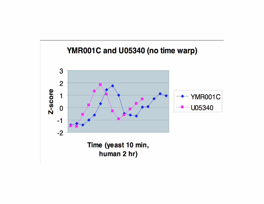
•  time series data (eg cell cycle gene expression data)

Pareto chart and ogive from Wikipedia

Summary statistics

•  center of a distribution –  mean

–  mode (most frequently taken value) •  unimodal distribution •  bimodal distribution, multimodal distribution

–  median (middle value when data sorted) –  midrange: (max+min)/2 –  range: [min,max]

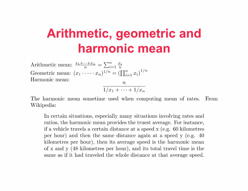
Arithmetic, geometric and harmonic mean

•  weighted mean

•  10% trimmed mean: remove bottom 10% and top 10% of data values and recompute mean for the remaining 80% of the original data set

•  skewedness: left and right skewed distributions (right skewed example of extreme value distribution from BLAST hits)

Example of extreme value distribution (a.k.a. Gumbel)

•  symmetric distribution: left and right half are mirror images -- technically if distribution function f is symmetric about the mean, i.e. f(µ+x)=f(µ-x)

•  different measures of center (mean, median, midrange, mode) affected differently by outliers

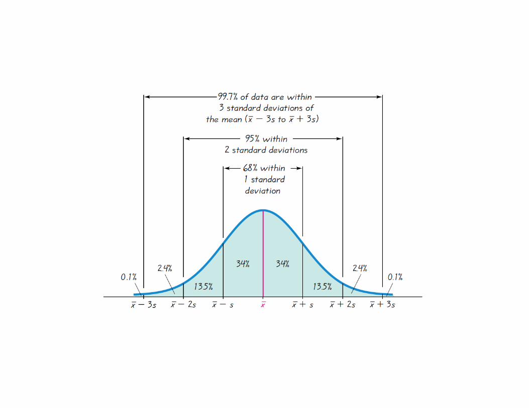
Normal distribution

Population Variance •  variation of a distribution

–  population variance: –  population standard deviation: sqrt(var)

–  Notation: –  population stdev and population variance:

Sample Variance •  variation of a sample

–  Sample variance: var –  population standard deviation: sqrt(var) –  Notation:

–  Sample stdev and sample variance: s, s2

Derivation of shortcut formula

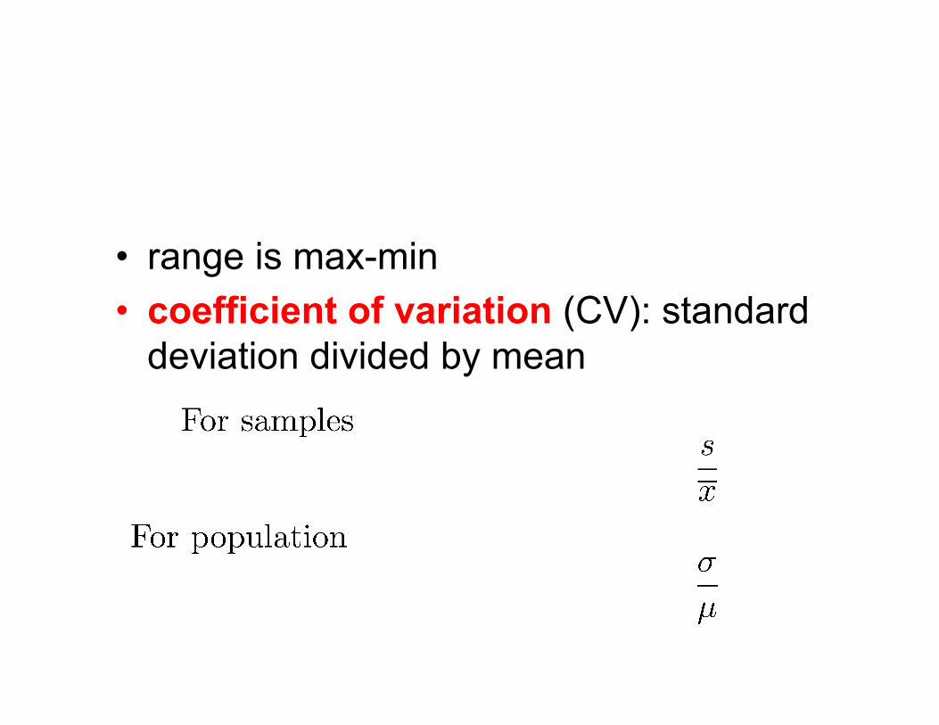
•  range is max-min •  coefficient of variation (CV): standard

deviation divided by mean

Mean absolute deviation (essentially never used)

Range rule of thumb

•  For approximately normally distributed data, standard deviation is roughly range/4

•  For approximately normally distributed data, – min ¼ µ - 2 σ – max ¼ µ + 2 σ

Z-scores •  standardization: number of standard

deviations to left or right

•  range rule of thumb based on fact that for approximately normally distributed data -2 < z-score < +2

Area under bell-shaped curve between -2 and +2 is 0.954499736 Area under bell-shaped curve between -1 and +1 is 0.682689492

Quartiles •  first quartile: data value x such that {y: y<x}

constitutes bottom 25% of data •  second quartile: data value x such that {y:

y<x} constitutes bottom 50% of data •  third quartile: data value x such that {y: y<x}

constitutes bottom 75% of data

No uniform agreement on method to determine quartiles

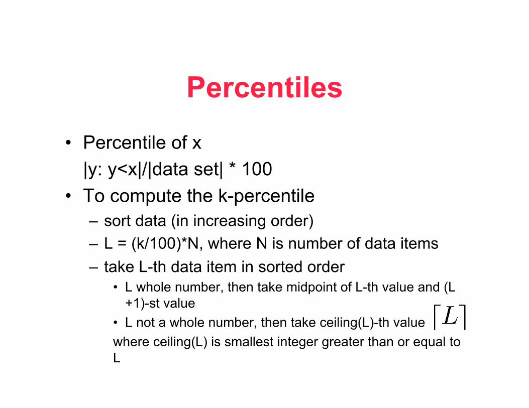
Percentiles

•  Percentile of x |y: y<x|/|data set| * 100

•  To compute the k-percentile –  sort data (in increasing order) –  L = (k/100)*N, where N is number of data items –  take L-th data item in sorted order

•  L whole number, then take midpoint of L-th value and (L+1)-st value

•  L not a whole number, then take ceiling(L)-th value where ceiling(L) is smallest integer greater than or equal to L

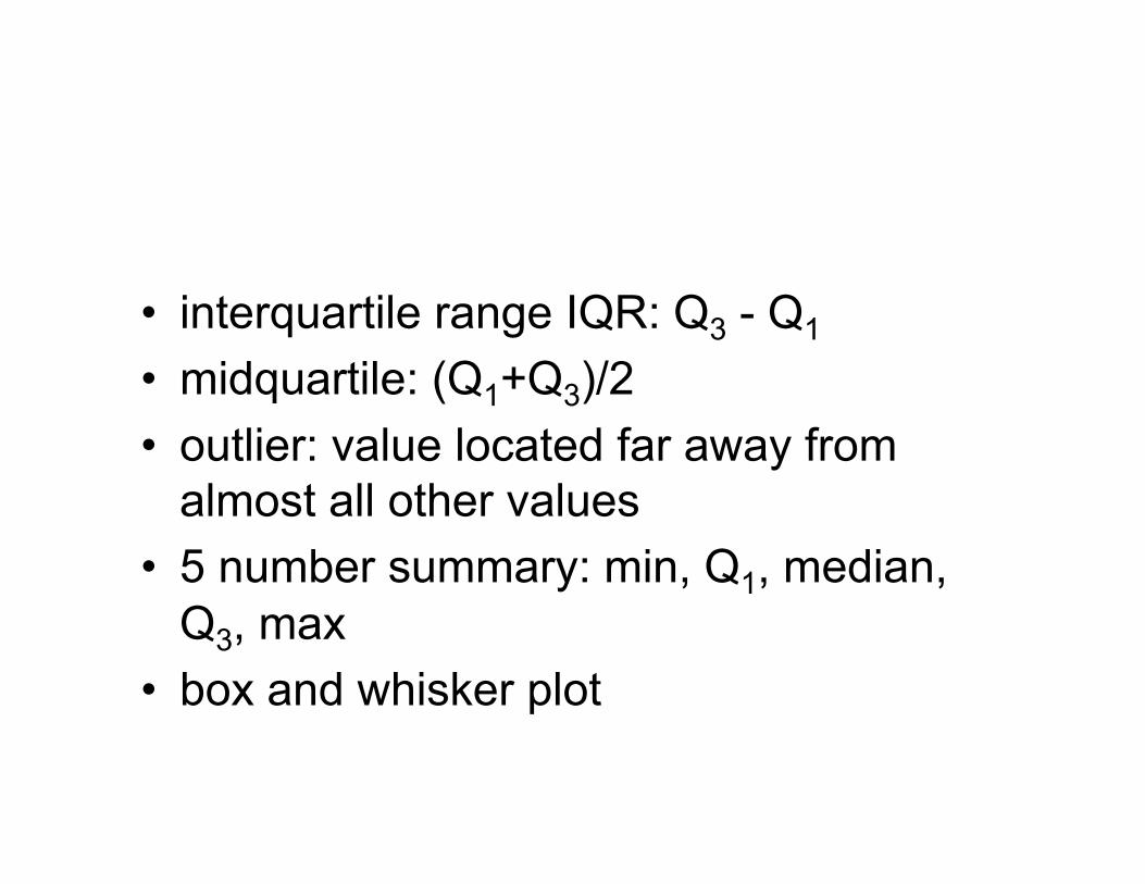
•  interquartile range IQR: Q3 - Q1 •  midquartile: (Q1+Q3)/2 •  outlier: value located far away from

almost all other values •  5 number summary: min, Q1, median,

Q3, max •  box and whisker plot

Box and whiskers plot from Wikipedia.

Creating a histogram with Excel

Column A contains 53 bear ages, in A1:A55 (only the first 12 ages are shown). You create upper class limits for bin values. Now select C2:C11 (one more row than bin values), and type frequency(A2:A54,B2:B10), and then APPLE+ENTER

To make histogram: select frequency values in C1:C10 (not C11 since this is overflow). Choose tab CHART, then column chart (far left tab) and create the histogram. To ensure that class upper limits appear on x-axis instead of 1,2,3,... right click the graph, choose to select data, then click small rectangular box to right of blank for category (x-axis) labels. In dialogue box that appears, drag click A2:A10 and ENTER. You can change title and further modify.

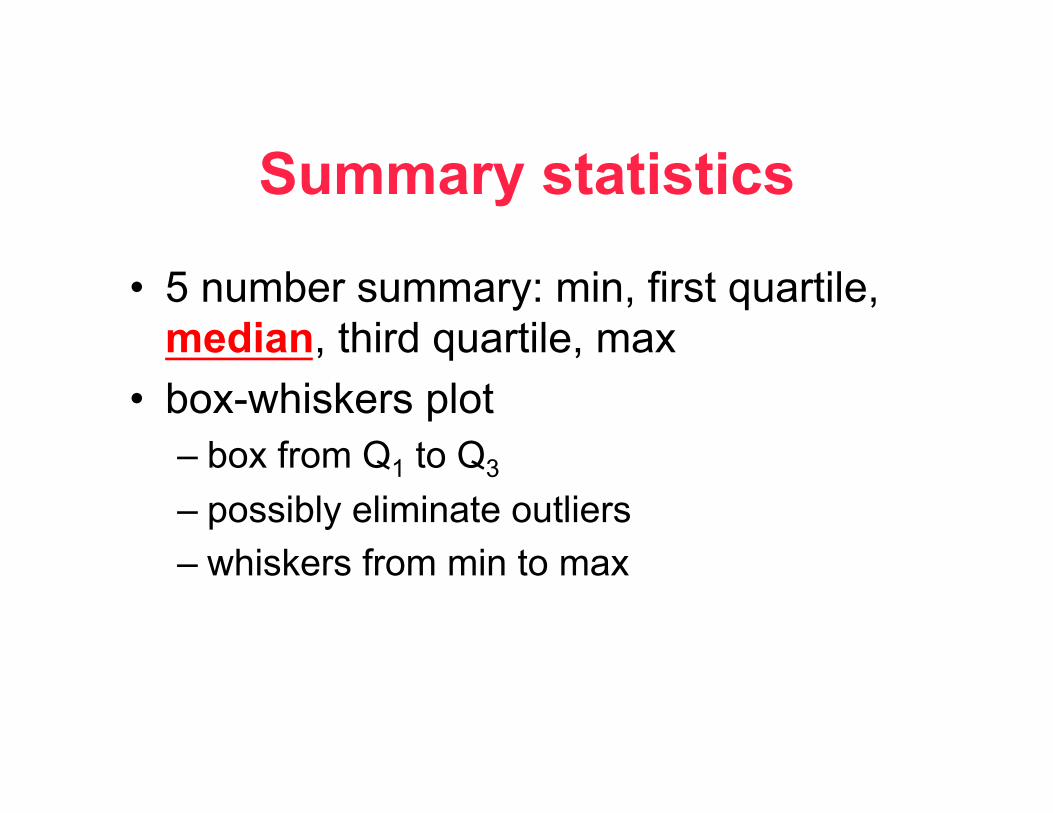
Summary statistics

•  5 number summary: min, first quartile, median, third quartile, max

•  box-whiskers plot – box from Q1 to Q3 – possibly eliminate outliers – whiskers from min to max

Excel statistical functions

•  average •  mode •  stdev •  stdevp •  var •  varp •  max,min,median

•  QUARTILE –  Returns the quartile of a data set (quartile =

0,1,2,3,4) –  Syntax: QUARTILE(array,quart)

•  PERCENTILE –  Returns the k-th percentile of values in a range. For

example, you can decide to examine candidates who score above the 90th percentile.

–  Syntax: PERCENTILE(array,k) Here k is in interval [0,1] e.g. 0.9.

•  STANDARDIZE –  Returns Z-score corresponding to x for a distribution with

mean and stdev. –  Syntax: STANDARDIZE(x,mean,stdev)

•  BINOMDIST – Returns the individual term binomial

distribution probability. – Syntax: BINOMDIST(k,n,p,cumulative). Used for sampling with replacement Density function when cumulative = false Cumulative density function when cumulative = true

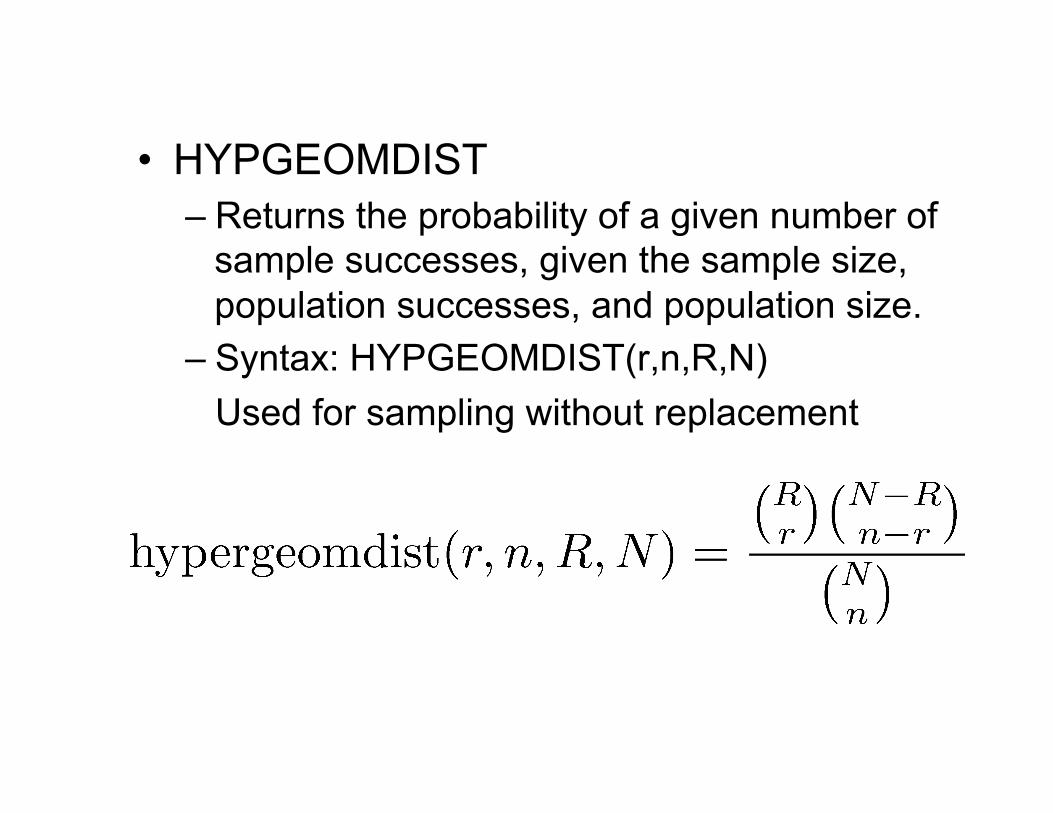
•  HYPGEOMDIST – Returns the probability of a given number of

sample successes, given the sample size, population successes, and population size.

– Syntax: HYPGEOMDIST(r,n,R,N) Used for sampling without replacement

•  PERMUT – Returns the number of ORDERED

sequences of length k drawn from a set of size n. Permutations are different from combinations, for which order is not significant.

– Syntax: PERMUT(n,k)

•  fact(k) – Returns the factorial k(k-1)(k-2)...1 – use permut and fact to compute

combinations

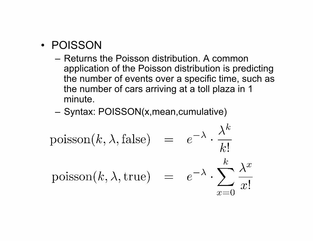
•  POISSON –  Returns the Poisson distribution. A common

application of the Poisson distribution is predicting the number of events over a specific time, such as the number of cars arriving at a toll plaza in 1 minute.

–  Syntax: POISSON(x,mean,cumulative)

•  NORMDIST –  Returns the normal distribution for the specified mean and

standard deviation. –  Syntax: NORMDIST(x,mean,stdev,cumulative)

•  NORMDIST –  Returns the normal distribution for the specified mean and standard

deviation. –  Syntax: NORMDIST(x,mean,stdev,cumulative)

•  NORMSINV –  Returns the inverse of the standard normal cumulative distribution.

The distribution has a mean of zero and a standard deviation of one. –  Syntax: NORMSINV(probability)