chapter15 systemtheoryandanalytical techniques
TRANSCRIPT

Chapter 15
System Theory and AnalyticalTechniques
Steven M. LaValle
University of Illinois
Copyright Steven M. LaValle 2006
Available for downloading at http://planning.cs.uiuc.edu/
Published by Cambridge University Press

Chapter 15
System Theory and AnalyticalTechniques
This chapter is complementary to Chapter 14 in that it provides tools and conceptsthat can be used to develop better local planning methods (LPMs). Most of thematerial was developed in the field of control theory, which focuses mainly oncharacterizing the behavior of particular classes of systems, and controlling themin the absence of obstacles. The two-point boundary value problem (BVP), whichwas a frequent nuisance in Chapter 14, can be better understood and solved formany systems by using the ideas of this chapter. Keep in mind that throughoutthis chapter there are no obstacles. Although planning for this case was trivial inPart II, the presence of differential constraints brings many challenges.
The style in this chapter is to provide a brief survey of concepts and techniques,with the hope of inspiring further study in other textbooks and research litera-ture. Modern control theory is a vast and fascinating subject, of which only thesurface can be scratched in one chapter. Section 15.1 introduces stability and con-trollability concepts, both of which characterize possible arrivals in a goal state.Stability characterizes how the integral curves of a vector field behave around agoal point, and controllability indicates whether an action trajectory exists thatarrives at a specified goal.
Section 15.2 revisits dynamic programming one last time. Here it becomes apartial differential equation expressed in terms of the optimal cost-to-go function.In some cases, it actually has a closed-form solution, as opposed to its main usein computer science, which is to obtain algorithm constraints. The powerful Pon-tryagin’s minimum principle, which can be derived from dynamic programming,is also covered.
The remainder of the chapter is devoted to nonholonomic systems, which oftenarise from underactuated mechanical systems. Section 15.3 expresses the shortestpaths between any pair of points for the Dubins car, the Reeds-Shepp car, anda differential drive, all of which were introduced in Section 13.1.2. The pathsare a beautiful solution to the BVP and are particularly valuable as an LPM; for
861
862 S. M. LaValle: Planning Algorithms
example, some have been used in the plan-and-transform method of Section 14.6.2.Section 15.4 addresses some basic properties of nonholonomic systems. The mostimportant issues are determining whether nonholonomic constraints are actuallyintegrable (which removes all xi variables) and characterizing reachable sets thatarise due to nonholonomic constraints. Section 15.5 attempts to do the same asSection 15.3, but for more challenging nonholonomic systems. In these cases, theBVP problem may not be solved optimally, and some methods may not even reachthe goal point precisely. Nevertheless, when applicable, they can be used to buildpowerful LPMs in a sampling-based motion planning algorithm.
15.1 Basic System Properties
This section provides a brief overview of two fundamental concepts in controltheory: stability and controllability. Either can be considered as characterizinghow a goal state is reached. Stability usually involves feedback and may onlyconverge to the goal as time approaches infinity. Controllability assesses whetheran action trajectory exists that leads exactly to a specified goal state. In bothcases, there is no obstacle region in X.
15.1.1 Stability
The subject of stability addresses properties of a vector field with respect to agiven point. Let X denote a smooth manifold on which the vector field is defined;X may be a C-space or a phase space. The given point is denoted as xG andcan be interpreted in motion planning applications as the goal state. Stabilitycharacterizes how xG is approached from other states in X by integrating thevector field.
The given vector field f is considered as a velocity field, which is representedas
x = f(x). (15.1)
This looks like a state transition equation that is missing actions. If a system ofthe form x = f(x, u) is given, then u can be fixed by designing a feedback planπ : X → U . This yields x = f(x, π(x)), which is a vector field on X without anyfurther dependency on actions. The dynamic programming approach in Section14.5 computed such a solution. The process of designing a stable feedback plan isreferred to in control literature as feedback stabilization.
Equilibrium points and Lyapunov stability At the very least, it seems thatthe state should remain fixed at xG, if it is reached. A point xG ∈ X is calledan equilibrium point (or fixed point) of the vector field f if and only if f(xG) = 0.This does not, however, characterize how trajectories behave in the vicinity of xG.

15.1. BASIC SYSTEM PROPERTIES 863
xG
O1
O1
xI
xG
O2
(a) (b)
Figure 15.1: Lyapunov stability: (a) Choose any open set O1 that contains xG,and (b) there exists some open set O2 from which trajectories will not be able toescape O1. Note that convergence to xG is not required.
Let xI ∈ X denote some initial state, and let x(t) refer to the state obtained attime t after integrating the vector field f from xI = x(0).
See Figure 15.1. An equilibrium point xG ∈ X is called Lyapunov stable if forany open neighborhood1 O1 of xG there exists another open neighborhood O2 ofxG such that xI ∈ O2 implies that x(t) ∈ O1 for all t > 0. If X = R
n, then someintuition can be obtained by using an equivalent definition that is expressed interms of the Euclidean metric. An equilibrium point xG ∈ R
n is called Lyapunovstable if, for any t > 0, there exists some δ > 0 such that ‖xI − xG‖ < δ impliesthat ‖x(t) − xG‖ < ǫ. This means that we can choose a ball around xG with aradius as small as desired, and all future states will be trapped within this ball,as long as they start within a potentially smaller ball of radius δ. If a single δcan be chosen independently of every ǫ and x, then the equilibrium point is calleduniform Lyapunov stable.
Asymptotic stability Lyapunov stability is weak in that it does not even implythat x(t) converges to xG as t approaches infinity. The states are only requiredto hover around xG. Convergence requires a stronger notion called asymptoticstability. A point xG is an asymptotically stable equilibrium point of f if:
1. It is a Lyapunov stable equilibrium point of f .
2. There exists some open neighborhood O of xG such that, for any xI ∈ O,x(t) converges2 to xG as t approaches infinity.
For X = Rn, the second condition can be expressed as follows: There exists some
δ > 0 such that, for any xI ∈ X with ‖xI−xG‖ < δ, the state x(t) converges to xGas t approaches infinity. It may seem strange that two requirements are needed
1An open neighborhood of a point x means an open set that contains x.2This convergence can be evaluated using the metric ρ on X.
864 S. M. LaValle: Planning Algorithms
for asymptotic stability. The first one bounds the amount of wiggling room forthe integral curve, which is not captured by the second condition.
Asymptotic stability appears to be a reasonable requirement, but it does notimply anything about how long it takes to converge. If xG is asymptotically stableand there exist some m > 0 and α > 0 such that
‖x(t)− xG‖ ≤ me−αt‖xI − xG‖, (15.2)
then xG is also called exponentially stable. This provides a convenient way toexpress the rate of convergence.
For use in motion planning applications, even exponential convergence maynot seem strong enough. This issue was discussed in Section 8.4.1. For example,in practice, one usually prefers to reach xG in finite time, as opposed to onlybeing “reached” in the limit. There are two common fixes. One is to allowasymptotic stability and declare the goal to be reached if the state arrives insome small, predetermined ball around xG. In this case, the enlarged goal willalways be reached in finite time if xG is asymptotically stable. The other fix is torequire a stronger form of stability in which xG must be exactly reached in finitetime. To enable this, however, discontinuous vector fields such as the inward flowof Figure 8.5b must be used. Most control theorists are appalled by this becauseinfinite energy is usually required to execute such trajectories. On the other hand,discontinuous vector fields may be a suitable representation in some applications,as mentioned in Chapter 8. Note that without feedback this issue does not seem asimportant. The state trajectories designed in much of Chapter 14 were expectedto reach the goal in finite time. Without feedback there was no surrounding vectorfield that was expected to maintain continuity or smoothness properties. Section15.1.3 introduces controllability, which is based on actually arriving at the goalin finite time, but it is also based on the existence of one trajectory for a givensystem x = f(x, u), as opposed to a family of trajectories for a given vector fieldx = f(x).
Time-varying vector fields The stability notions expressed here are usuallyintroduced in the time-varying setting x = f(x, t). Since the vast majority ofplanning problems in this book are time-invariant, the presentation was confinedto time-invariant vector fields. There is, however, one fascinating peculiarity inthe topic of finding a feedback plan that stabilizes a system. Brockett’s conditionimplies that for some time-invariant systems for which continuous, time-varyingfeedback plans exist, there does not exist a continuous time-invariant feedbackplan [20, 23, 90]. This includes the class of driftless control systems, such as thesimple car and the unicycle. This implies that to maintain continuity of the vectorfield, a time dependency must be introduced to allow the vector field to vary as xGis approached! If continuity of the vector field is not important, then this concernvanishes.

15.1. BASIC SYSTEM PROPERTIES 865
Domains of attraction The stability definitions given so far are often calledlocal because they are expressed in terms of a neighborhood of xG. Global versionscan also be defined by extending the neighborhood to all of X. An equilibriumpoint is globally asymptotically stable if it is Lyapunov stable, and the integralcurve from any x0 ∈ X converges to xG as time approaches infinity. It may be thecase that only points in some proper subset of X converge to xG. The set of allpoints in X that converge to xG is often called the domain of attraction of xG. Thefunnels of Section 8.5.1 are based on domains of attraction. Also related is thebackward reachable set from Section 14.2.1. In that setting, action trajectorieswere considered that lead to xG in finite time. For the domain of attraction onlyasymptotic convergence to xG is assumed, and the vector field is given (there areno actions to choose).
Limit cycles For some vector fields, states may be attracted into a limit cycle.Rather than stabilizing to a point, the state trajectories converge to a loop pathin X. For example, they may converge to following a circle. This occurs in a widevariety of mechanical systems in which oscillations are possible. Some of the basicissues, along with several interesting examples for X = R
2, are covered in [5].
15.1.2 Lyapunov Functions
Suppose a velocity field x = f(x) is given along with an equilibrium point, xG.Can the various forms of stability be easily determined? One of the most powerfulmethods to prove stability is to construct a Lyapunov function. This will beintroduced shortly, but first some alternatives are briefly mentioned.
If f(x) is linear, which means that f(x) = Ax for some constant n× n matrixA and X = R
n, then stability questions with respect to the origin, xG = 0, areanswered by finding the eigenvalues of A [25]. The state x = 0 is asymptoticallystable if and only if all eigenvalues of A have negative real parts. Consider thescalar case, x = ax, for which X = R and a is a constant. The solution tothis differential equation is x(t) = x(0) eat, which converges to 0 only if a < 0.This can be easily extended to the case in which X = R
n and A is an n × ndiagonal matrix for which each diagonal entry (or eigenvalue) is negative. Fora general matrix, real or complex eigenvalues determine the stability (complexeigenvalues cause oscillations). Conditions also exist for Lyapunov stability. Everyequilibrium state of x = Ax is Lyapunov stable if the eigenvalues of A all havenonpositive real parts, and the eigenvalues with zero real parts are distinct rootsof the characteristic polynomial of A.
If f(x) is nonlinear, then stability can sometimes be inferred by linearizingf(x) about xG and performing linear stability analysis. In many cases, however,this procedure is inconclusive (see Chapter 6 of [23]). Proving the stability of avector field is a challenging task for most nonlinear systems. One approach isbased on LaSalle’s invariance principle [4, 23, 54] and is particularly useful for
866 S. M. LaValle: Planning Algorithms
showing convergence to any of multiple goal states (see Section 5.4 of [75]). Theother major approach is to construct a Lyapunov function, which is used as anintermediate tool to indirectly establish stability. If this method fails, then it stillmay be possible to show stability using other means. Therefore, it is a sufficientcondition for stability, but not a necessary one.
Determining stability Suppose a velocity field x = f(x) is given along withan equilibrium point xG. Let φ denote a candidate Lyapunov function, which willbe used as an auxiliary device for establishing the stability of f . An appropriateφ must be determined for the particular vector field f . This may be quite chal-lenging in itself, and the details are not covered here. In a sense, the procedurecan be characterized as “guess and verify,” which is the way that many solutiontechniques for differential equations are described. If φ succeeds in establishingstability, then it is promoted to being called a Lyapunov function for f .
It will be important to characterize how φ varies in the direction of flow inducedby f . This is measured by the Lie derivative,
φ(x) =n∑
i=1
∂φ
∂xifi(x). (15.3)
This results in a new function φ(x), which indicates for each x the change in φalong the direction of x = f(x).
Several concepts are needed to determine stability. Let a function h : [0,∞) →[0,∞) be called a hill if it is continuous, strictly increasing, and h(0) = 0. Thiscan be considered as a one-dimensional navigation function, which has a singlelocal minimum at the goal, 0. A function φ : X → [0,∞) is called locally positivedefinite if there exists some open set O ⊆ X and a hill function h such thatφ(xG) = 0 and φ(x) ≥ h(‖x‖) for all x ∈ O. If O can be chosen as O = X, andif X is bounded, then φ is called globally positive definite or just positive definite.In some spaces this may not be possible due to the topology of X; such issuesarose when constructing navigation functions in Section 8.4.4. If X is unbounded,then h must additionally approach infinity as ‖x‖ approaches infinity to yield apositive definite φ [75]. For X = R
n, a quadratic form xTMx, for which M is apositive definite matrix, is a globally positive definite function. This motivatesthe use of quadratic forms in Lyapunov stability analysis.
The Lyapunov theorems can now be stated [23, 75]. Suppose that φ is locallypositive definite at xG. If there exists an open set O for which xG ∈ O, andφ(x) ≤ 0 on all x ∈ O, then f is Lyapunov stable. If −φ(x) is also locally positivedefinite on O, then f is asymptotically stable. If φ and −φ are both globallypositive definite, then f is globally asymptotically stable.
Example 15.1 (Establishing Stability via Lyapunov Functions) LetX =R. Let x = f(x) = −x5, and we will attempt to show that x = 0 is stable. Let thecandidate Lyapunov function be φ(x) = 1
2x2. The Lie derivative (15.3) produces

15.1. BASIC SYSTEM PROPERTIES 867
φ(x) = −x6. It is clear that φ and −φ are both globally positive definite; hence,0 is a global, asymptotically stable equilibrium point of f . �
Lyapunov functions in planning Lyapunov functions are closely related tonavigation functions and optimal cost-to-go functions in planning. In the optimaldiscrete planning problem of Sections 2.3 and 8.2, the cost-to-go values can beconsidered as a discrete Lyapunov function. By applying the computed actions,a kind of discrete vector field can be imagined over the search graph. Each ap-plied optimal action yields a reduction in the optimal cost-to-go value, until 0is reached at the goal. Both the optimal cost-to-go and Lyapunov functions en-sure that the trajectories do not become trapped in a local minimum. Lyapunovfunctions are more general than cost-to-go functions because they do not requireoptimality. They are more like navigation functions, as considered in Chapter8. The requirements for a discrete navigation function, as given in Section 8.2.2,are very similar to the positive definite condition given in this section. Imaginethat the navigation function shown in Figure 8.3 is a discrete approximation toa Lyapunov function over R
2. In general, a Lyapunov function indicates someform of distance to xG, although it may not be optimal. Nevertheless, it is basedon making monotonic progress toward xG. Therefore, it may serve as a distancefunction in many sampling-based planning algorithms of Chapter 14. Since it re-spects the differential constraints imposed by the system, it may provide a betterindication of how to make progress during planning in comparison to a Euclideanmetric that ignores these considerations. Lyapunov functions should be particu-larly valuable in the RDT method of Section 14.4.3, which relies heavily on thedistance function over X.
15.1.3 Controllability
Now suppose that a system x = f(x, u) is given on a smooth manifold X asdefined throughout Chapter 13 and used extensively in Chapter 14. The systemcan be considered as a parameterized family of vector fields in which u is theparameter. For stability, it was assumed that this parameter was fixed by afeedback plan to obtain some x = f(x). This section addresses controllability,which indicates whether one state is reachable from another via the existence ofan action trajectory u. It may be helpful to review the reachable set definitionsfrom Section 14.2.1.
Classical controllability Let U denote the set of permissible action trajectoriesfor the system, as considered in Section 14.1.1. By default, this is taken as anyu for which (14.1) can be integrated. A system x = f(x, u) is called controllableif for all xI , xG ∈ X, there exists a time t > 0 and action trajectory u ∈ U suchthat upon integration from x(0) = xI , the result is x(t) = xG. Controllability can
868 S. M. LaValle: Planning Algorithms
alternatively be expressed in terms of the reachable sets of Section 14.2.1. Thesystem is controllable if xG ∈ R(xI ,U) for all xI , xG ∈ X.
A system is therefore controllable if a solution exists to any motion planningproblem in the absence of obstacles. In other words, a solution always exists tothe two-point boundary value problem (BVP).
Example 15.2 (Classical Controllability) All of the vehicle models in Sec-tion 13.1.2 are controllable. For example, in an infinitely large plane, the Dubinscar can be driven between any two configurations. Note, however, that if theplane is restricted by obstacles, then this is not necessarily possible with the Du-bins car. As an example of a system that is not controllable, let X = R, x = u,and U = [0, 1]. In this case, the state cannot decrease. For example, there existsno action trajectory that brings the state from xI = 1 to xG = 0. �
Many methods for determining controllability of a system are covered in stan-dard textbooks on control theory. If the system is linear, as given by (13.37) withdimensions m and n, then it is controllable if and only if the n×nm controllabilitymatrix
M = [B... AB
... A2B... · · ·
... An−1B] (15.4)
has full rank [25]. This is called the Kalman rank condition [47]. If the system isnonlinear, then the controllability matrix can be evaluated on a linearized versionof the system. Having full rank is sufficient to establish controllability from asingle point (see Proposition 11.2 in [75]). If the rank is not full, however, thesystem may still be controllable. A fascinating property of some nonlinear systemsis that they may be able to produce motions in directions that do not seem tobe allowed at first. For example, the simple car given in Section 13.1.2 cannotslide sideways; however, it is possible to wiggle the car sideways by performingparallel-parking maneuvers. A method for determining the controllability of suchsystems is covered in Section 15.4.
For fully actuated systems of the form q = h(q, q, u), controllability can bedetermined by converting the system into double-integrator form, as consideredin Section 14.4.1. Let the system be expressed as q = u′, in which u′ ∈ U ′(q, q). IfU ′(q, q) contains an open neighborhood of the origin of Rn, and the same neigh-borhood can be used for any x ∈ X, then the system is controllable. If a nonlinearsystem is underactuated, as in the simple car, then controllability issues becomeconsiderably more complicated. The next concept is suitable for such systems.
STLC: Controllability that handles obstacles The controllability conceptdiscussed so far has no concern for how far the trajectory travels in X before xGis reached. This issue becomes particularly important for underactuated systemsand planning among obstacles. These concerns motivate a natural question: Isthere a form of controllability that is naturally suited for obstacles? It should

15.1. BASIC SYSTEM PROPERTIES 869
xI
B(xI , ǫ)
int(R(xI ,U , t′))
Figure 15.2: If the system is STLC, then motions can be made in any direction,in an arbitrarily small amount of time.
declare that if a state is reachable from another in the absence of differentialconstraints, then it is also reachable with the given system x = f(x, u). This canbe expressed using time-limited reachable sets. Let R(x,U , t) denote the set ofall states reachable in time less than or equal to t, starting from x. A systemx = f(x, u) is called small-time locally controllable (STLC) from xI if there existssome t > 0 such that xI ∈ int(R(xI ,U , t
′)) for all t′ ∈ (0, t] (here, int denotes theinterior of a set, as defined in Section 4.1.1). If the system x = f(x, u) is STLCfrom every xI ∈ X, then the whole system is said to be STLC.
Consider using this definition to answer the question above. Since int(R(xI ,U , t′))
is an open set, there must exist some small ǫ > 0 for which the open ball B(xI , ǫ)is a strict subset of int(R(xI ,U , t
′)). See Figure 15.2. Any point on the boundaryof B(xI , ǫ) can be reached, which means that a step of size ǫ can be taken in anydirection, even though differential constraints exist. With obstacles, however, wehave to be careful that the trajectory from xI to the surface of B(xI , ǫ) does notwander too far away.
Suppose that there is an obstacle region Xobs, and a violation-free state trajec-tory x is given that terminates in xG at time tF and does not necessarily satisfya given system. If the system is STLC, then it is always possible to find an-other trajectory, based on x, that satisfies the differential constraints. Apply theplan-and-transform method of Section 14.6.2. Suppose that intervals for potentialreplacement are chosen using binary recursive subdivision. Also suppose that anLPM exists that computes that shortest trajectory between any pair of states;this trajectory ignores obstacles but respects the differential constraints. Initially,[0, tF ] is replaced by a trajectory from the LPM, and if it is not violation-free, then[0, tF ] is subdivided into [0, tF/2] and [tF/2, tF ], and replacement is attempted onthe smaller intervals. This idea can be applied recursively until eventually thesegments are small enough that they must be violation-free.
This final claim is implied by the STLC property. No matter how small theintervals become, there must exist a replacement trajectory. If an interval islarge, then there may be sufficient time to wander far from the original trajectory.However, as the time interval decreases, there is not enough time to deviate far
870 S. M. LaValle: Planning Algorithms
from the original trajectory. (This discussion assumes mild conditions on f , suchas being Lipschitz.) Suppose that the trajectory is protected by a collision-freetube of radius ǫ. Thus, all points along the trajectory are at least ǫ from theboundary of Xfree. The time intervals can be chosen small enough to ensure thatthe trajectory deviations are less than ǫ from the original trajectory. Therefore,STLC is a very important property for a system to possess for planning in thepresence of obstacles. Section 15.4 covers some mathematical tools for determiningwhether a nonlinear system is STLC.
A concept closely related to controllability is accessibility, which is only con-cerned with the dimension of the reachable set. Let n be the dimension of X. Ifthere exists some t > 0 for which the dimension of R(xI ,U , t) is n, then the systemis called accessible from xI . Alternatively, this may be expressed as requiring thatint(R(xI ,U , t)) 6= ∅.
Example 15.3 (Accessibility) Recall the system from Section 13.1.3 in whichthe state is trapped on a circle. In this case X = R
2, and the state transitionequation was specified by x = yu and y = −xu. This system is not accessiblebecause the reachable sets have dimension one. �
A small-time version of accessibility can also be defined by requiring that thereexists some t such that int(R(xI ,U , t
′)) 6= ∅ for all t′ ∈ (0, t]. Accessibility isparticularly important for systems with drift.
15.2 Continuous-Time Dynamic Programming
Dynamic programming has been a recurring theme throughout most of this book.So far, it has always taken the form of computing optimal cost-to-go (or cost-to-come) functions over some sequence of stages. Both value iteration and Dijkstra-like algorithms have emerged. In computer science, dynamic programming is afundamental insight in the development of algorithms that compute optimal so-lutions to problems. In its original form, however, dynamic programming wasdeveloped to solve the optimal control problem [10]. In this setting, a discreteset of stages is replaced by a continuum of stages, known as time. The dy-namic programming recurrence is instead a partial differential equation, calledthe Hamilton-Jacobi-Bellman (HJB) equation. The HJB equation can be solvedusing numerical algorithms; however, in some cases, it can be solved analytically.3
Section 15.2.2 briefly describes an analytical solution in the case of linear systems.Section 15.2.3 covers Pontryagin’s minimum principle, which can be derived fromthe dynamic programming principle, and generalizes the optimization performedin Hamiltonian mechanics (recall Section 13.4.4).
3It is often surprising to computer scientists that dynamic programming in this case does notyield an algorithm. It instead yields a closed-form solution to the problem.

15.2. CONTINUOUS-TIME DYNAMIC PROGRAMMING 871
15.2.1 Hamilton-Jacobi-Bellman Equation
The HJB equation is a central result in optimal control theory. Many otherprinciples and design techniques follow from the HJB equation, which itself is justa statement of the dynamic programming principle in continuous time. A properderivation of all forms of the HJB equation would be beyond the scope of thisbook. Instead, a time-invariant formulation that is most relevant to planning willbe given here. Also, an informal derivation will follow, based in part on [12].
The discrete case
Before entering the continuous realm, the concepts will first be described for dis-crete planning, which is often easier to understand. Recall from Section 2.3 thatif X, U , and the stages are discrete, then optimal planning can be performed byusing value iteration or Dijkstra’s algorithm on the search graph. The stationary,optimal cost-to-go function G∗ can be used as a navigation function that encodesthe optimal feedback plan. This was suggested in Section 8.2.2, and an examplewas shown in Figure 8.3.
Suppose that G∗ has been computed under Formulation 8.1 (or Formulation2.3). Let the state transition equation be denoted as
x′ = fd(x, u). (15.5)
The dynamic programming recurrence for G∗ is
G∗(x) = minu∈U(x)
{l(x, u) +G∗(x′)} , (15.6)
which may already be considered as a discrete form of the Hamilton-Jacobi-Bellman equation. To gain some insights into the coming concepts, however,some further manipulations will be performed.
Let u∗ denote the optimal action that is applied in the min of (15.6). Imaginethat u∗ is hypothesized as the optimal action but needs to be tested in (15.6) tomake sure. If it is truly optimal, then
G∗(x) = l(x, u∗) +G∗(fd(x, u∗)). (15.7)
This can already be considered as a discrete form of the Pontryagin minimumprinciple, which will appear in Section 15.2.3. By rearranging terms, a nice inter-pretation is obtained:
G∗(fd(x, u∗))−G∗(x) = −l(x, u∗). (15.8)
In a single stage, the optimal cost-to-go drops by l(x, u∗) when G∗ is used asa navigation function (multiply (15.8) by −1). The optimal single-stage costis revealed precisely when taking one step toward the goal along the optimalpath. This incremental change in the cost-to-go function while moving in the bestdirection forms the basis of both the HJB equation and the minimum principle.
872 S. M. LaValle: Planning Algorithms
The continuous case
Now consider adapting to the continuous case. Suppose X and U are both con-tinuous, but discrete stages remain, and verify that (15.5) to (15.8) still hold true.Their present form can be used for any system that is approximated by discretestages. Suppose that the discrete-time model of Section 14.2.2 is used to approxi-mate a system x = f(x, u) on a state space X that is a smooth manifold. In thatmodel, U was discretized to Ud, but here it will be left in its original form. Let∆t represent the time discretization.
The HJB equation will be obtained by approximating (15.6) with the discrete-time model and letting ∆t approach zero. The arguments here are very informal;see [12, 51, 84] for more details. Using discrete-time approximation, the dynamicprogramming recurrence is
G∗(x) = minu∈U(x)
{ld(x, u) +G∗(x′)} , (15.9)
in which ld is a discrete-time approximation to the cost that accumulates overstage k and is given as
ld(x, u) ≈ l(x, u)∆t. (15.10)
It is assumed that as ∆t approaches zero, the total discretized cost converges tothe integrated cost of the continuous-time formulation.
Using the linear part of a Taylor series expansion about x, the term G∗(x′)can be approximated as
G∗(x′) ≈ G∗(x) +n∑
i=1
∂G∗
∂xifi(x, u)∆t. (15.11)
This approximates G∗(x′) by its tangent plane at x. Substitution of (15.11) and(15.10) into (15.9) yields
G∗(x) ≈ minu∈U(x)
{
l(x, u)∆t+G∗(x) +n∑
i=1
∂G∗
∂xifi(x, u)∆t
}
. (15.12)
Subtracting G∗(x) from both sides of (15.12) yields
minu∈U(x)
{
l(x, u)∆t+n∑
i=1
∂G∗
∂xifi(x, u)∆t
}
≈ 0. (15.13)
Taking the limit as ∆t approaches zero and then dividing by ∆t yields the HJBequation:
minu∈U(x)
{
l(x, u) +n∑
i=1
∂G∗
∂xifi(x, u)
}
= 0. (15.14)

15.2. CONTINUOUS-TIME DYNAMIC PROGRAMMING 873
Compare the HJB equation to (15.6) for the discrete-time case. Both indicatehow the cost changes when moving in the best direction. Substitution of u∗ forthe optimal action into (15.14) yields
n∑
i=1
∂G∗
∂xifi(x, u
∗) = −l(x, u∗). (15.15)
This is just the continuous-time version of (15.8). In the current setting, the leftside indicates the derivative of the cost-to-go function along the direction obtainedby applying the optimal action from x.
The HJB equation, together with a boundary condition that specifies the final-stage cost, sufficiently characterizes the optimal solution to the planning problem.Since it is expressed over the whole state space, solutions to the HJB equationyield optimal feedback plans. Unfortunately, the HJB equation cannot be solvedanalytically in most settings. Therefore, numerical techniques, such as the valueiteration method of Section 14.5, must be employed. There is, however, an im-portant class of problems that can be directly solved using the HJB equation; seeSection 15.2.2.
Variants of the HJB equation
Several versions of the HJB equation exist. The one presented in (15.14) is suitablefor planning problems such as those expressed in Chapter 14. If the cost-to-gofunctions are time-dependent, then the HJB equation is
minu∈U(x)
{
l(x, u, t) +∂G∗
∂t+
n∑
i=1
∂G∗
∂xifi(x, u, t)
}
= 0, (15.16)
and G∗ is a function of both x and t. This can be derived again using a Taylorexpansion, but with x and t treated as the variables. Most textbooks on optimalcontrol theory present the HJB equation in this form or in a slightly different formby pulling ∂G∗/∂t outside of the min and moving it to the right of the equation:
minu∈U(x)
{
l(x, u, t) +n∑
i=1
∂G∗
∂xifi(x, u, t)
}
= −∂G∗
∂t. (15.17)
In differential game theory, the HJB equation generalizes to the Hamilton-Jacobi-Isaacs (HJI) equations [6, 43]. Suppose that the system is given as (13.203)and a zero-sum game is defined using a cost term of the form l(x, u, v, t). The HJIequations characterize saddle equilibria and are given as
minu∈U(x)
maxv∈V (x)
{
l(x, u, v, t) +∂G∗
∂t+
n∑
i=1
∂G∗
∂xifi(x, u, v, t)
}
= 0 (15.18)
874 S. M. LaValle: Planning Algorithms
and
maxv∈V (x)
minu∈U(x)
{
l(x, u, v, t) +∂G∗
∂t+
n∑
i=1
∂G∗
∂xifi(x, u, v, t)
}
= 0. (15.19)
There are clear similarities between these equations and (15.16). Also, the swap-ping of the min and max operators resembles the definition of saddle points inSection 9.3.
15.2.2 Linear-Quadratic Problems
This section briefly describes a problem for which the HJB equation can be directlysolved to yield a closed-form expression, as opposed to an algorithm that computesnumerical approximations. Suppose that a linear system is given by (13.37), whichrequires specifying the matrices A and B. The task is to design a feedback planthat asymptotically stabilizes the system from any initial state. This is an infinite-horizon problem, and no termination action is applied.
An optimal solution is requested with respect to a cost functional based onmatrix quadratic forms. Let Q be a nonnegative definite4 n × n matrix, and letR be a positive definite n× n matrix. The quadratic cost functional is defined as
L(x, u) =1
2
∫ ∞
0
(
x(t)TQx(t) + u(t)TRu(t))
dt. (15.20)
To guarantee that a solution exists that yields finite cost, several assumptions mustbe made on the matrices. The pair (A,B) must be stabilizable, and (A,Q) mustbe detectable; see [2] for specific conditions and a full derivation of the solutionpresented here.
Although it is not done here, the HJB equation can be used to derive thealgebraic Riccati equation,
SA+ ATS − SBR−1BTS +Q = 0, (15.21)
in which all matrices except S were already given. Methods exist that solve forS, which is a unique solution in the space of nonnegative definite n× n matrices.
The linear vector field
x =(
A−BR−1BTS)
x (15.22)
is asymptotically stable (the real parts of all eigenvalues of the matrix are nega-tive). This vector field is obtained if u is selected using a feedback plan π definedas
π(x) = −R−1BTSx. (15.23)
4Nonnegative definite means xTQx ≥ 0 for all x ∈ R, and positive definite means xTRx > 0for all x ∈ R
n.

15.2. CONTINUOUS-TIME DYNAMIC PROGRAMMING 875
The feedback plan π is in fact optimal, and the optimal cost-to-go is simply
G∗(x) = 12xTSx. (15.24)
Thus, for linear systems with quadratic cost, an elegant solution exists withoutresorting to numerical approximations. Unfortunately, the solution techniques donot generalize to nonlinear systems or linear systems among obstacles. Hence, theplanning methods of Chapter 14 are justified.
However, many variations and extensions of the solutions given here do exist,but only for other problems that are expressed as linear systems with quadraticcost. In every case, some variant of Riccati equations is obtained by application ofthe HJB equation. Solutions to time-varying systems are derived in [2]. If there isGaussian uncertainty in predictability, then the linear-quadratic Gaussian (LQG)problem is obtained [50]. Linear-quadratic problems and solutions even exist fordifferential games of the form (13.204) [6].
15.2.3 Pontryagin’s Minimum Principle
Pontryagin’s minimum principle5 is closely related to the HJB equation and pro-vides conditions that an optimal trajectory must satisfy. Keep in mind, however,that the minimum principle provides necessary conditions, but not sufficient con-ditions, for optimality. In contrast, the HJB equation offered sufficient conditions.Using the minimum principle alone, one is often not able to conclude that a tra-jectory is optimal. In some cases, however, it is quite useful for finding candidateoptimal trajectories. Any trajectory that fails to satisfy the minimum principlecannot be optimal.
To understand the minimum principle, we first return to the case of discreteplanning. As mentioned previously, the minimum principle is essentially givenby (15.7). This can be considered as a specialization of the HJB equation to thespecial case of applying the optimal action u∗. This causes the min to disappear,but along with it the global properties of the HJB equation also vanish. Theminimum principle expresses conditions along the optimal trajectory, as opposedto the cost-to-go function over the whole state space. Therefore, it can at bestassure local optimality in the space of possible trajectories.
The minimum principle for the continuous case is essentially given by (15.15),which is the continuous-time counterpart to (15.7). However, it is usually ex-pressed in terms of adjoint variables and a Hamiltonian function, in the spirit ofHamiltonian mechanics from Section 13.4.4.
Let λ denote an n-dimensional vector of adjoint variables, which are definedas
λi =∂G∗
∂xi. (15.25)
5This is often called Pontryagin’s maximum principle, because Pontryagin originally defined itas a maximization [71]. The Hamiltonian used in most control literature is negated with respectto Pontryagin’s Hamiltonian; therefore, it becomes minimized. Both names are in common use.
876 S. M. LaValle: Planning Algorithms
The Hamiltonian function is defined as
H(x, u, λ) = l(x, u) +n∑
i=1
λifi(x, u), (15.26)
which is exactly the expression inside of the min of the HJB equation (15.14) afterusing the adjoint variable definition from (15.25). This can be compared to theHamiltonian given by (13.192) in Section 13.4.4 (p from that context becomes λhere). The two are not exactly the same, but they both are motivated by thesame basic principles.
Under the execution of the optimal action trajectory u∗, the HJB equationimplies that
H(x(t), u∗(t), λ(t)) = 0 (15.27)
for all t ≥ 0. This is just an alternative way to express (15.15). The fact that Hremains constant appears very much like a conservation law, which was the basisof Hamiltonian mechanics in Section 13.4.4. The use of the Hamiltonian in theminimum principle is more general.
Using the HJB equation (15.14), the optimal action is given by
u∗(t) = argminu∈U(x)
{H(x(t), u(t), λ(t))} . (15.28)
In other words, the Hamiltonian is minimized precisely at u(t) = u∗(t).The missing piece of information so far is how λ evolves over time. It turns
out that a system of the form
λ = g(x, λ, u∗) (15.29)
can be derived by differentiating the Hamiltonian (or, equivalently, the HJB equa-tion) with respect to x. This yields two coupled systems, x = f(x, u∗) and (15.29).These can in fact be interpreted as a single system in a 2n-dimensional phase space,in which each phase vector is (x, λ). This is analogous to the phase interpretationin Section 13.4.4 for Hamiltonian mechanics, which results in (13.198).
Remember that λ is defined in (15.25) just to keep track of the change in G∗. Itwould be helpful to have an explicit form for (15.29). Suppose that u∗ is selectedby a feedback plan to yield u∗ = π∗(x). In this case, the Hamiltonian can beinterpreted as a function of only x and λ. Under this assumption, differentiatingthe Hamiltonian (15.26) with respect to xi yields
∂l(x, π∗(x))
∂xi+
n∑
j=1
∂λj∂xi
fj(x, π∗(x)) +
n∑
j=1
λj∂fj(x, π
∗(x))
∂xi. (15.30)
This validity of this differentiation requires a technical lemma that asserts thatthe derivatives of π(x) can be disregarded (see Lemma 3.3.1 of [12]). Also, it will

15.2. CONTINUOUS-TIME DYNAMIC PROGRAMMING 877
be assumed that U is convex in the arguments that follow, even though there existproofs of the minimum principle that do not require this.
The second term in (15.30) is actually λi, although it is hard to see at first.The total differential of λi with respect to the state is
dλi =n∑
j=1
∂λi∂xj
dxj. (15.31)
Dividing both sides by dt yields
dλidt
=n∑
j=1
∂λi∂xj
dxjdt
=n∑
j=1
∂λi∂xj
xj. (15.32)
Each xj is given by the state transition equation: xj = fj(x, π∗(x)). Therefore,
λi =dλidt
=d
dt
∂G∗
∂xi=
n∑
j=1
∂λi∂xj
fj(x, π∗(x)). (15.33)
Substituting (15.33) into (15.30) and setting the equation to zero (because theHamiltonian is zero along the optimal trajectory) yields
∂l(x, π∗(x))
∂xi+ λi +
n∑
j=1
λj∂fj(x, π
∗(x))
∂xi= 0. (15.34)
Solving for λi yields
λi = −∂l(x, π∗(x))
∂xi−
n∑
j=1
λj∂fj(x, π
∗(x))
∂xi. (15.35)
Conveniently, this is the same as
λi = −∂H
∂xi, (15.36)
which yields the adjoint transition equation, as desired.The transition equations given by x = f(x, u) and (15.36) specify the evolution
of the system given by the minimum principle. These are analogous to Hamil-ton’s equations (13.198), which were given in Section 13.4.4. The generalizedmomentum in that context becomes the adjoint variables here.
When applying the minimum principle, it is usually required to use the factthat the optimal action at all times must satisfy (15.28). Often, this is equivalentlyexpressed as
H(x(t), u∗(t), λ(t)) ≤ H(x(t), u(t), λ(t)), (15.37)
which indicates that the Hamiltonian increases or remains the same wheneverdeviation from the optimal action occurs (the Hamiltonian cannot decrease).
878 S. M. LaValle: Planning Algorithms
Example 15.4 (Optimal Planning for the Double Integrator) Recall thedouble integrator system from Example 13.3. Let q = u, C = R, and U =[−1, 1] ∪ {uT}. Imagine a particle that moves in R. The action is a force in ei-ther direction and has at most unit magnitude. The state transition equation isx1 = x2 and x2 = u, and X = R
2. The task is to perform optimal motion planningbetween any two states xI , xG ∈ X. From a given initial state xI , a goal state xGmust be reached in minimum time. The cost functional is defined in this case asl(x, u) = 1 for all x ∈ X and and u ∈ U such that u 6= uT .
Using (15.26), the Hamiltonian is defined as
H(x, u, λ) = 1 + λ1x2 + λ2u. (15.38)
The optimal action trajectory is obtained from (15.28) as
u∗(t) = argminu∈[−1,1]
{1 + λ1(t)x2(t) + λ2(t)u(t)} . (15.39)
If λ2(t) < 0, then u∗(t) = 1, and if λ2(t) > 0, then u∗(t) = −1. Thus, the actionmay be assigned as u∗(t) = −sgn(λ2(t)), if λ2(t) 6= 0. Note that these two casesare the “bangs” of the bang-bang control from Section 14.6.3, and they are alsothe extremal actions used for the planning algorithm in Section 14.4.1. At theboundary case in which λ2(t) = 0, any action in [−1, 1] may be chosen.
The only remaining task is to determine the values of the adjoint variablesover time. The adjoint transition equation is obtained from (15.36) as λ1 = 0 andλ2 = −λ1. The solutions are λ1(t) = c1 and λ2(t) = c2−c1t, in which c1 and c2 areconstants that can be determined at t = 0 from (15.38) and (15.39). The optimalaction depends only on the sign of λ2(t). Since its solution is the equation of aline, it can change signs at most once. Therefore, there are four possible kinds ofsolutions, depending on the particular xI and xG:
1. Pure acceleration, u∗(t) = 1, is applied for all time.
2. Pure deceleration, u∗(t) = −1, is applied for all time.
3. Pure acceleration is applied up to some time t′ and is followed immediatelyby pure deceleration until the final time.
4. Pure deceleration is applied up to some time t′ followed immediately by pureacceleration until the final time.
For the last two cases, t′ is often called the switching time, at which point a dis-continuity in u∗ occurs. These two are bang-bang solutions, which were describedin Section 14.6.3. �
This was one of the simplest possible examples, and the optimal solution waseasily found because the adjoint variables are linear functions of time. Section 15.3

15.2. CONTINUOUS-TIME DYNAMIC PROGRAMMING 879
covers optimal solutions for the Dubins car, the Reeds-Shepp car, and the differ-ential drive, all of which can be established using the minimum principle combinedwith some geometric arguments. As systems become more complicated, such anal-ysis is unfortunately too difficult. In these cases, sampling-based methods, suchas those of Chapter 14, must be used to determine optimal trajectories.
One common complication is the existence of singular arcs along the solutiontrajectory. These correspond to a degeneracy in H with respect to u over someduration of time. This could be caused, for example, by having H independent ofu. In Example 15.4, H became independent of u when λ2(t) = 0; however, therewas no singular arc because this could only occur for an instant of time. If theduration had been longer, then there would be an interval of time over which theoptimal action could not be determined. In general, if the Hessian (recall definitionfrom (8.48)) of H with respect to u is a positive definite matrix, then there are nosingular arcs (this is often called the Legendre-Clebsch condition). The minimumprinciple in this case provides a sufficient condition for local optimality in thespace of possible state trajectories. If the Hessian is not positive definite for someinterval [t1, t2] with t1 < t2, then additional information is needed to determinethe optimal trajectory over the singular arc from x∗(t1) to x∗(t2).
Note that all of this analysis ignores the existence of obstacles. There is noth-ing to prevent the solutions from attempting to enter an obstacle region. Theaction set U(x) and cost l(x, u) can be adjusted to account for obstacles; however,determining an optimal solution from the minimum principle becomes virtuallyimpossible, except in some special cases.
There are other ways to derive the minimum principle. Recall from Section13.4.4 that Hamilton’s equations can be derived from the Euler-Lagrange equa-tion. It should not be surprising that the minimum principle can also be derivedusing variational principles [12, 69]. The minimum principle can also be inter-preted as a form of constrained optimization. This yields the interpretation ofλ as Lagrange multipliers. A very illuminating reference for further study of theminimum principle is Pontryagin’s original works [71].
Time optimality Interesting interpretations of the minimum principle exist forthe case of optimizing the time to reach the goal [40, 82]. In this case, l(x, u) = 1in (15.26), and the cost term can be ignored. For the remaining portion, let λ bedefined as
λi = −∂G∗
∂xi, (15.40)
instead of using (15.25). In this case, the Hamiltonian can be expressed as
H(x, u, λ) =n∑
i=1
λifi(x, u) =
⟨
−∂G∗
∂x, f(x, u)
⟩
, (15.41)
which is an inner product between f(x, u) and the negative gradient of G∗. Using(15.40), the Hamiltonian should be maximized instead of minimized (this is equiv-
880 S. M. LaValle: Planning Algorithms
alent to Pontryagin’s original formulation [71]). An inner product of two vectorsincreases as their directions become closer to parallel. Optimizing (15.41) amountsto selecting u so that x is as close as possible to the direction of steepest descent ofG∗. This is nicely interpreted by considering how the boundary of the reachableset R(x0,U , t) propagates through X. By definition, the points on ∂R(x0,U , t)must correspond to time-optimal trajectories. Furthermore, ∂R(x0,U , t) can beinterpreted as a propagating wavefront that is perpendicular to −∂G∗/∂x. Theminimum principle simply indicates that u should be chosen so that x points intothe propagating boundary, as close to being orthogonal as possible [40].
15.3 Optimal Paths for Some Wheeled Vehicles
For some of the wheeled vehicle models of Section 13.1.2, the shortest path betweenany pair of configurations was completely characterized. In this section, X = C =R
2×S1, which corresponds to the C-space for a rigid body in the plane. For each
model, the path length in C must be carefully defined to retain some physicalsignificance in the world W = R
2 in which the vehicle travels. For example, inthe case of the simple car, the distance in W traveled by the center of the rearaxle will be optimized. If the coordinate frame is assigned appropriately, thiscorresponds to optimizing the path length in the R2 subspace of C while ignoringorientation. Keep in mind that the solutions given in this section depend heavilyon the particular cost functional that is optimized.
Sections 15.3.1–15.3.3 cover the shortest paths for the Dubins car, the Reeds-Shepp car, and a differential-drive model, respectively. In each case, the pathscan be elegantly described as combinations of a few motion primitives. Due tosymmetries, it is sufficient to describe the optimal paths from a fixed initial con-figuration qI = (0, 0, 0) to any goal configuration qG ∈ C. If the optimal path isdesired from a different qI ∈ C, then it can be recovered from rigid-body transfor-mations applied to qI and qG (the whole path can easily be translated and rotatedwithout effecting its optimality, provided that qG does not move relative to qI).Alternatively, it may be convenient to fix qG and consider optimal paths from allpossible qI .
Once qI (or qG) is fixed, C can be partitioned into cells that correspond to setsof placements for qG (or qI). Inside of each cell, the optimal curve is described bya fixed sequence of parameterized motion primitives. For example, one cell for theDubins car indicates “turn left,” “go straight,” and then “turn right.” The curvesare ideally suited for use as an LPM in a sampling-based planning algorithm.
This section mainly focuses on presenting the solutions. Establishing theircorrectness is quite involved and is based in part on Pontryagin’s minimum prin-ciple from Section 15.2.3. Other important components are Filipov’s existencetheorem (see [82]) and Boltyanskii’s sufficient condition for optimality (which alsojustifies dynamic programming) [16]. Substantially more details and justificationsof the curves presented in Sections 15.3.1 and 15.3.2 appear in [82, 83, 85]. The

15.3. OPTIMAL PATHS FOR SOME WHEELED VEHICLES 881
Symbol Steering: u
S 0L 1R -1
Figure 15.3: The three motion primitives from which all optimal curves for theDubins car can be constructed.
corresponding details for the curves of Section 15.3.3 appear in [8].
15.3.1 Dubins Curves
Recall the Dubins version of the simple car given in Section 13.1.2. The system wasspecified in (13.15). It is assumed here that the car moves at constant forwardspeed, us = 1. The other important constraint is the maximum steering angleφmax, which results in a minimum turning radius ρmin. As the car travels, considerthe length of the curve in W = R
2 traced out by a pencil attached to the centerof the rear axle. This is the location of the body-frame origin in Figure 13.1. Thetask is to minimize the length of this curve as the car travels between any qI andqG. Due to ρmin, this can be considered as a bounded-curvature shortest-pathproblem. If ρmin = 0, then there is no curvature bound, and the shortest pathfollows a straight line in R
2. In terms of a cost functional of the form (8.39), thecriterion to optimize is
L(q, u) =
∫ tF
0
√
x(t)2 + y(t)2dt, (15.42)
in which tF is the time at which qG is reached, and a configuration is denoted asq = (x, y, θ). If qG is not reached, then it is assumed that L(q, u) = ∞.
Since the speed is constant, the system can be simplified to
x = cos θ
y = sin θ
θ = u,
(15.43)
in which u is chosen from the interval U = [− tanφmax, tanφmax]. This impliesthat (15.42) reduces to optimizing the time tF to reach qG because the integrandreduces to 1. For simplicity, assume that tanφ = 1. The following results alsohold for any φmax ∈ (0, π/2).
It was shown in [32] that between any two configurations, the shortest pathfor the Dubins car can always be expressed as a combination of no more thanthree motion primitives. Each motion primitive applies a constant action over aninterval of time. Furthermore, the only actions that are needed to traverse the
882 S. M. LaValle: Planning Algorithms
α
γ
dRα
Sd
Lγ
qGqIα
γ
Rγ
Rα
qGqI
Lβ
β
RαSdLγ RαLβRγ
Figure 15.4: The trajectories for two words are shown in W = R2.
shortest paths are u ∈ {−1, 0, 1}. The primitives and their associated symbolsare shown in Figure 15.3. The S primitive drives the car straight ahead. The Land R primitives turn as sharply as possible to the left and right, respectively.Using these symbols, each possible kind of shortest path can be designated as asequence of three symbols that corresponds to the order in which the primitivesare applied. Let such a sequence be called a word . There is no need to havetwo consecutive primitives of the same kind because they can be merged into one.Under this observation, ten possible words of length three are possible. Dubinsshowed that only these six words are possibly optimal:
{LRL, RLR, LSL, LSR, RSL, RSR}. (15.44)
The shortest path between any two configurations can always be characterized byone of these words. These are called the Dubins curves.
To be more precise, the duration of each primitive should also be specified.For L or R, let a subscript denote the total amount of rotation that accumulatesduring the application of the primitive. For S, let a subscript denote the totaldistance traveled. Using such subscripts, the Dubins curves can be more preciselycharacterized as
{LαRβ Lγ, Rα Lβ Rγ, Lα Sd Lγ, Lα SdRγ, Rα Sd Lγ , Rα SdRγ}, (15.45)
in which α, γ ∈ [0, 2π), β ∈ (π, 2π), and d ≥ 0. Figure 15.4 illustrates two cases.Note that β must be greater than π (if it is less, then some other word becomesoptimal).
It will be convenient to invent a compressed form of the words to group togetherpaths that are qualitatively similar. This will be particularly valuable when Reeds-Shepp curves are introduced in Section 15.3.2 because there are 46 of them, asopposed to 6 Dubins curves. Let C denote a symbol that means “curve,” andrepresents either R or L. Using C, the six words in (15.44) can be compressed to

15.3. OPTIMAL PATHS FOR SOME WHEELED VEHICLES 883
y
x
LSR RSL
RSL LSR
LSL
RSR
LRL
RLR
Figure 15.5: A slice at θ = π of the partition into word-invariant cells for theDubins car. The circle is centered on the origin.
only two base words:{CCC, CSC}. (15.46)
In this compressed form, remember that two consecutive Cs must be filled in bydistinct turns (RR and LL are not allowed as subsequences). In compressed form,the base words can be specified more precisely as
{CαCβ Cγ, Cα SdCγ}, (15.47)
in which α, γ ∈ [0, 2π), β ∈ (π, 2π), and d ≥ 0.Powerful information has been provided so far for characterizing the shortest
paths; however, for a given qI and qG, two problems remain:
1. Which of the six words in (15.45) yields the shortest path between qI andqG?
2. What are the values of the subscripts, α, β, γ, and d for the particular word?
To use the Dubins curves as an LPM, these questions should be answered effi-ciently. One simple approach is to try all six words and choose the shortest one.The parameters for each word can be determined by tracing out minimum-radiuscircles from qI and qG, as shown in Figure 14.23. Another way is to use the precisecharacterization of the regions over which a particular word is optimal. Supposethat qG is fixed at (0, 0, 0). Based on the possible placements of qI , the C-spacecan be partitioned into cells for which the same word is optimal. The cells andtheir boundaries are given precisely in [82]. As an example, a slice of the celldecomposition for θ = π is shown in Figure 15.5.
884 S. M. LaValle: Planning Algorithms
Figure 15.6: Level sets of the Dubins metric are shown in the plane. Along twocircular arcs, the metric is discontinuous (courtesy of Philippe Soueres).
In addition to use as an LPM, the resulting cost of the shortest path may bea useful distance function in many sampling-based planning algorithms. This issometimes called the Dubins metric (it is not, however, a true metric because itviolates the symmetry axiom). This can be considered as the optimal cost-to-goG∗. It could have been computed approximately using the dynamic programmingapproach in Section 14.5; however, thanks to careful analysis, the exact values areknown. One interesting property of the Dubins metric is that it is discontinuous;see Figure 15.6. Compare the cost of traveling π/2 using the R primitive to thecost of traveling to a nearby point that would require a smaller turning radiusthan that achieved by the R primitive. The required action does not exist in U ,and the point will have to be reached by a longer sequence of primitives. Thediscontinuity in G∗ is enabled by the fact that the Dubins car fails to possess theSTLC property from Section 15.1.3. For STLC systems, G∗ is continuous.
15.3.2 Reeds-Shepp Curves
Now consider the shortest paths of the Reeds-Shepp car. The only differencein comparison to the Dubins car is that travel in the reverse direction is nowallowed. The same criterion (15.42) is optimized, which is the distance traveledby the center of the rear axle. The shortest path is equivalent to the path thattakes minimum time, as for the Dubins car. The simplified system in (15.43) canbe enhanced to obtain
x = u1 cos θ
y = u1 sin θ
θ = u1u2,
(15.48)
in which u1 ∈ {−1, 1} and u2 ∈ [− tanφmax, tanφmax]. The first action variable,u1, selects the gear, which is forward (u1 = 1) or reverse (u1 = −1). Once again,

15.3. OPTIMAL PATHS FOR SOME WHEELED VEHICLES 885
Base α β γ d
Cα|Cβ|Cγ [0, π] [0, π] [0, π] −Cα|CβCγ [0, β] [0, π/2] [0, β] −CαCβ|Cγ [0, β] [0, π/2] [0, β] −CαSdCγ [0, π/2] - [0, π/2] (0,∞)CαCβ|CβCγ [0, β] [0, π/2] [0, β] −Cα|CβCβ|Cγ [0, β] [0, π/2] [0, β] −Cα|Cπ/2SdCπ/2|Cγ [0, π/2] - [0, π/2] (0,∞)Cα|Cπ/2SdCγ [0, π/2] - [0, π/2] (0,∞)CαSdCπ/2|Cγ [0, π/2] - [0, π/2] (0,∞)
Figure 15.7: The interval ranges are shown for each motion primitive parameterfor the Reeds-Shepp optimal curves.
assume for simplicity that u2 ∈ [−1, 1]. The results stated here apply to anyφmax ∈ (0, π/2).
It was shown in [73] that there are no more than 48 different words thatdescribe the shortest paths for the Reeds-Shepp car. The base word notation fromSection 15.3.1 can be extended to nicely express the shortest paths. A new symbol,“ | ”, is used in the words to indicate that the “gear” is shifted from forward toreverse or reverse to forward. Reeds and Shepp showed that the shortest path fortheir car can always be expressed with one of the following base words:
{C|C|C, CC|C, C|CC, CSC, CCβ|Cβ C, C|Cβ Cβ|C,
C|Cπ/2SC, CSCπ/2|C, C|Cπ/2SCπ/2|C}.(15.49)
As many as five primitives could be needed to execute the shortest path. Asubscript of π/2 is given in some cases because the curve must be followed forprecisely π/2 radians. For some others, β is given as a subscript to indicate thatit must match the parameter of another primitive. The form given in (15.49)is analogous to (15.46) for the Dubins car. The parameter ranges can also bespecified, to yield a form analogous to (15.47). The result is shown in Figure 15.7.Example curves for two cases are shown in Figure 15.9.
Now the base words will be made more precise by specifying the particularmotion primitive. Imagine constructing a list of words analogous to (15.44) forthe Dubins car. There are six primitives as shown in Figure 15.8. The symbolsS, L, and R are used again. To indicate the forward or reverse gear, + and −superscripts will be used as shown in Figure 15.8.6
Figure 15.10 shows 48 different words, which result from uncompressing thebase words expressed using C, S, and “ | ” in (15.49). Each shortest path is a
6This differs conceptually from the notation used in [82]. There, r− corresponds to L− here.The L here means that the steering wheel is positioned for a left turn, but the car is in reverse.This aids in implementing the rule that R and L cannot be consecutive in a word.
886 S. M. LaValle: Planning Algorithms
Symbol Gear: u1 Steering: u2
S+ 1 0S− -1 0L+ 1 1L− -1 1R+ 1 -1R− -1 -1
Figure 15.8: The six motion primitives from which all optimal curves for theReeds-Shepp car can be constructed.
α
γ
qGqI
β
R+α R+
γ
L−
β
Figure 15.9: An example of the R+αL
−βR
+γ curve. This uses reverse to generate a
curve that is shorter than the one in Figure 15.4b for the Dubins car.
word with length at most five. There are substantially more words than for theDubins car. Each base word in (15.49) expands into four or eight words using themotion primitives. To uncompress each base word, the rule that R and L cannotbe applied consecutively is maintained. This yields four possibilities for the firstsix compressed words. The remaining three involve an intermediate S primitive,which allows eight possible sequences of Rs and Ls for each one. Two of the 48words were eliminated in [85]. Each of the remaining 46 words can actually occurfor a shortest path and are called the Reeds-Shepp curves.
For use as an LPM, the problem appears once again of determining the partic-ular word and parameters for a given qI and qG. This was not difficult for Dubinscurves, but now there are 46 possibilities. The naive approach of testing everyword and choosing the shortest one may be too costly. The precise cell boundariesin C over which each word applies are given in [82]. The cell boundaries are un-fortunately quite complicated, which makes the point location algorithm difficult

15.3. OPTIMAL PATHS FOR SOME WHEELED VEHICLES 887
Base word Sequences of motion primitivesC|C|C (L+R−L+)(L−R+L−)(R+L−R+)(R−L+R−)CC|C (L+R+L−)(L−R−L+)(R+L+R−)(R−L−R+)C|CC (L+R−L−)(L−R+L+)(R+L−R−)(R−L+R+)CSC (L+S+L+)(L−S−L−)(R+S+R+)(R−S−R−)
(L+S+R+)(L−S−R−)(R+S+L+)(R−S−L−)CCβ|Cβ C (L+R+
β L−βR
−)(L−R−β L
+βR
+)(R+L+βR
−β L
−)(R−L−βR
+β L
+)
C|Cβ Cβ|C (L+R−β L
−βR
+)(L−R+β L
+βR
−)(R+L−βR
−β L
+)(R−L+βR
+β L
−)
C|Cπ/2SC (L+R−π/2S
−R−)(L−R+π/2S
+R+)(R+L−π/2S
−L−)(R−L+π/2S
+L+)
(L+R−π/2S
−L−)(L−R+π/2S
+L+) (R+L−π/2S
−R−)(R−L+π/2S
+R+)
CSCπ/2|C (L+S+L+π/2R
−)(L−S−L−π/2R
+)(R+S+R+π/2L
−)(R−S−R−π/2L
+)
(R+S+L+π/2R
−)(R−S−L−π/2R
+)(L+S+R+π/2L
−)(L−S−R−π/2L
+)
C|Cπ/2SCπ/2|C (L+R−π/2S
−L−π/2R
+)(L−R+π/2S
+L+π/2R
−)
(R+L−π/2S
−R−π/2L
+)(R−L+π/2S
+R+π/2L
−)
Figure 15.10: The 48 curves of Reeds and Shepp. Sussmann and Tang [85] showedthat (L−R+L−) and (R−L+R−), which appear in the first row, can be eliminated.Hence, only 46 words are needed to describe the shortest paths.
to implement. A simple way to prune away many words from consideration isto use intervals of validity for θ. For some values of θ, certain compressed wordsare impossible as shortest paths. A convenient table of words that become activeover ranges of θ is given in [82]. Once again, the length of the shortest path canserve as a distance function in sampling-based planning algorithms. The resultingReeds-Shepp metric is continuous because the Reeds-Shepp car is STLC, whichwill be established in Section 15.4.
15.3.3 Balkcom-Mason Curves
In recent years, two more families of optimal curves have been determined [8, 26].Recall the differential-drive system from Section 13.1.2, which appears in manymobile robot systems. In many ways, it appears that the differential drive isa special case of the simple car. The expression of the system given in (13.17)can be made to appear identical to the Reeds-Shepp car system in (15.48). Forexample, letting r = 1 and L = 1 makes them equivalent by assigning uω = u1 anduψ = u1u2. Consider the distance traveled by a point attached to the center of thedifferential-drive axle using (15.42). Minimizing this distance for any qI and qG istrivial, as shown in Figure 13.4 of Section 13.1.2. The center point can be made totravel in a straight line in W = R
2. This would be possible for the Reeds-Sheppcar if ρmin = 0, which implies that φmax = π/2. It therefore appeared for manyyears that no interesting curves exist for the differential drive.
The problem, however, with measuring the distance traveled by the axle centeris that pure rotations are cost-free. This occurs when the wheels rotate at the
888 S. M. LaValle: Planning Algorithms
Symbol Left wheel: ul Right wheel: ur
⇑ 1 1⇓ -1 -1x -1 1y 1 -1
Figure 15.11: The four motion primitives from which all optimal curves for thedifferential-drive robot can be constructed.
same speed but with opposite angular velocities. The center does not move;however, the time duration, energy expenditure, and wheel rotations that occurare neglected. By incorporating one or more of these into the cost functional, achallenging optimization arises. Balkcom and Mason bounded the speed of thedifferential drive and minimized the total time that it takes to travel from qI toqG. Using (13.16), the action set is defined as U = [−1, 1]× [−1, 1], in which themaximum rotation rate of each wheel is one (an alternative bound can be usedwithout loss of generality). The criterion to optimize is
L(q, u) =
∫ tF
0
√
x(t)2 + y(t)2 + |θ(t)|dt, (15.50)
which takes θ into account, whereas it was neglected in (15.42). This criterion isonce again equivalent to minimizing the time to reach qG. The resulting model willbe referred to as the Balkcom-Mason drive. An alternative criterion is the totalamount of wheel rotation; this leads to an alternative family of optimal curves[26].
It was shown in [8] that only the four motion primitives shown in Figure15.11 are needed to express time-optimal paths for the differential-drive robot.Each primitive corresponds to holding one action variable fixed at its limit foran interval of time. Using the symbols in Figure 15.11 (which were used in [8]),words can be formed that describe the optimal path. It has been shown that theword length is no more than five. Thus, any shortest paths may be expressed as apiecewise-constant action trajectory in which there are no more than five pieces.Every piece corresponds to one of the primitives in Figure 15.11.
It is convenient in the case of the Balkcom-Mason drive to use the same sym-bols for both base words and for precise specification of primitives. Symmetrytransformations will be applied to each base word to yield a family of eight wordsthat precisely specify the sequences of motion primitives. Nine base words describethe shortest paths:
{y, ⇓, ⇓y, y⇓y, ⇑xπ⇓, x⇓y, ⇓yy, x⇓y⇑, ⇑x⇓y⇑}. (15.51)
This is analogous to the compressed forms given in (15.46) and (15.49). Themotions are depicted in Figure 15.12.

15.3. OPTIMAL PATHS FOR SOME WHEELED VEHICLES 889
Figure 15.12: Each of the nine base words is depicted [8]. The last two are onlyvalid for small motions; they are magnified five times and the robot outline is notdrawn.
Base T1 T2 T3 T2 ◦ T1 T3 ◦ T1 T3 ◦ T2 T3 ◦ T2 ◦ T1A. y y y x y x x x
B. ⇓ ⇑ ⇓ ⇓ ⇑ ⇑ ⇓ ⇑
C. ⇓y ⇑y y⇓ ⇓x y⇑ ⇑x x⇓ x⇑
D. y⇓y y⇑y y⇓y x⇓x y⇑y x⇑x x⇓x x⇑x
E. ⇑xπ⇓ ⇓xπ⇑ ⇓xπ⇑ ⇑yπ⇓ ⇑xπ⇓ ⇓yπ⇑ ⇓yπ⇑ ⇑yπ⇓
F. x⇓y x⇑y y⇓x y⇓x y⇑x y⇑x x⇓y x⇑y
G. ⇓y⇑ ⇑y⇓ ⇑y⇓ ⇓x⇑ ⇓y⇑ ⇑x⇓ ⇑x⇓ ⇓x⇑
H. x⇓y⇑ x⇑y⇓ ⇑y⇓x y⇓x⇑ ⇓y⇑x y⇑x⇓ ⇑x⇓y ⇓x⇑y
I. ⇑x⇓y⇑ ⇓x⇑y⇓ ⇑y⇓x⇑ ⇑y⇓x⇑ ⇓y⇑x⇓ ⇓y⇑x⇓ ⇑x⇓y⇑ ⇓x⇑y⇓
Figure 15.13: The 40 optimal curve types for the differential-drive robot, sortedby symmetry class [8].
890 S. M. LaValle: Planning Algorithms
Figure 15.14: A slice of the optimal curves is shown for qI = (x, y, π4) and qG =
(0, 0, 0) [8]. Level sets of the optimal cost-to-go G∗ are displayed. The coordinatescorrespond to a differential drive with r = L = 1 in (13.16).
Figure 15.13 shows 40 distinct Balkcom-Mason curves that result from apply-ing symmetry transformations to the base words of (15.51). There are 72 entriesin Figure 15.13, but many are identical. The transformation T1 indicates thatthe directions of ⇑ and ⇓ are flipped from the base word. The transformation T2
reverses the order of the motion primitives. The transformation T3 flips the direc-tions of x and y. The transformations commute, and there are seven possibleways to combine them, which contributes to a row of Figure 15.13.
To construct an LPM or distance function, the same issues arise as for theReeds-Shepp and Dubins cars. Rather than testing all 40 words to find the shortestpath, simple tests can be defined over which a particular word becomes active[8]. A slice of the precise cell decomposition and the resulting optimal cost-to-go(which can be called the Balkcom-Mason metric) are shown in Figure 15.14.
15.4 Nonholonomic System Theory
This section gives some precision to the term nonholonomic, which was usedloosely in Chapters 13 and 14. Furthermore, small-time controllability (STLC),which was defined in Section 15.1.3, is addressed. The presentation given herebarely scratches the surface of this subject, which involves deep mathematicalprinciples from differential geometry, algebra, control theory, and mechanics. The

15.4. NONHOLONOMIC SYSTEM THEORY 891
intention is to entice the reader to pursue further study of these topics; see thesuggested literature at the end of the chapter.
15.4.1 Control-Affine Systems
Nonholonomic system theory is restricted to a special class of nonlinear systems.The techniques of Section 15.4 utilize ideas from linear algebra. The main conceptswill be formulated in terms of linear combinations of vector fields on a smoothmanifold X. Therefore, the formulation is restricted to control-affine systems,which were briefly introduced in Section 13.2.3. For these systems, x = f(x, u) isof the form
x = h0(x) +m∑
i=1
hi(x)ui, (15.52)
in which each hi is a vector field on X.
The vector fields are expressed using a coordinate neighborhood of X. Usually,m < n, in which n is the dimension of X. Unless otherwise stated, assume thatU = R
m. In some cases, U may be restricted.
Each action variable ui ∈ R can be imagined as a coefficient that determineshow much of hi(x) is blended into the result x. The drift term h0(x) alwaysremains and is often such a nuisance that the driftless case will be the main focus.This means that h0(x) = 0 for all x ∈ X, which yields
x =m∑
i=1
hi(x)ui. (15.53)
The driftless case will be used throughout most of this section. The set h1, . . .,hm, is referred to as the system vector fields. It is essential that U contains atleast an open set that contains the origin of Rm. If the origin is not contained inU , then the system is no longer driftless.7
Control-affine systems arise in many mechanical systems. Velocity constraintson the C-space frequently are of the Pfaffian form (13.5). In Section 13.1.1, it wasexplained that under such constraints, a configuration transition equation (13.6)can be derived that is linear if q is fixed. This is precisely the driftless form (15.53)using X = C. Most of the models in Section 13.1.2 can be expressed in this form.The Pfaffian constraints on configuration are often called kinematic constraintsbecause they arise due to the kinematics of bodies in contact, such as a wheelrolling. The more general case of (15.52) for a phase space X arises from dynamicconstraints that are obtained from Euler-Lagrange equation (13.118) or Hamilton’sequations (13.198) in the formulation of the mechanics. These constraints captureconservation laws, and the drift term usually appears due to momentum.
7Actually, if the convex hull of U contains an open set that contains the origin, then a driftlesssystem can be simulated by rapid switching.
892 S. M. LaValle: Planning Algorithms
Example 15.5 (A Simplified Model for Differential Drives and Cars) Boththe simple-car and the differential-drive models of Section 13.1.2 can be expressedin the form (15.53) after making simplifications. The simplified model, (15.48),can be adapted to conveniently express versions of both of them by using differentrestrictions to define U . The third equation of (15.48) can be reduced to θ = u2
without affecting the set of velocities that can be achieved. To conform to (15.53),the equations can then be written in a linear-algebra form as
xy
θ
=
cos θsin θ0
u1 +
001
u2. (15.54)
This makes it clear that there are two system vector fields, which can be combinedby selecting the scalar values u1 and u2. One vector field allows pure translation,and the other allows pure rotation. Without restrictions on U , this system be-haves like a differential drive because the simple car cannot execute pure rotation.Simulating the simple car with (15.54) requires restrictions on U (such as requir-ing that u1 be 1 or −1, as in Section 15.3.2). This is equivalent to the unicyclefrom Figure 13.5 and (13.18).
Note that (15.54) can equivalently be expressed as
xy
θ
=
cos θ 0sin θ 00 1
(
u1
u2
)
(15.55)
by organizing the vector fields into a matrix. �
In (15.54), the vector fields were written as column vectors that combine lin-early using action variables. This suggested that control-affine systems can bealternatively expressed using matrix multiplication in (15.55). In general, thevector fields can be organized into an n×m matrix as
H(x) =[
h1(x) h2(x) · · · hm(x)]
. (15.56)
In the driftless case, this yields
x = H(x) u (15.57)
as an equivalent way to express (15.53)It is sometimes convenient to work with Pfaffian constraints,
g1(x)x1 + g2(x)x2 + · · ·+ gn(x)xn = 0, (15.58)
instead of a state transition equation. As indicated in Section 13.1.1, a set of kindependent Pfaffian constraints can be converted into a state transition equation

15.4. NONHOLONOMIC SYSTEM THEORY 893
with m = (n − k) action variables. The resulting state transition equation isa driftless control-affine system. Thus, Pfaffian constraints provide a dual wayof specifying driftless control-affine systems. The k Pfaffian constraints can beexpressed in matrix form as
G(x) x = 0, (15.59)
which is the dual of (15.57), and G(x) is a k × n matrix formed from the gicoefficients of each Pfaffian constraint. Systems with drift can be expressed in aPfaffian-like form by constraints
g0(x) + g1(x)x1 + g2(x)x2 + · · ·+ gn(x)xn = 0. (15.60)
15.4.2 Determining Whether a System Is Nonholonomic
The use of linear algebra in Section 15.4.1 suggests further development of alge-braic concepts. This section briefly introduces concepts that resemble ordinarylinear algebra but apply to linear combinations of vector fields. This providesthe concepts and tools needed to characterize important system properties in theremainder of this section. This will enable the assessment of whether a system isnonholonomic and also whether it is STLC. Many of the constructions are namedafter Sophus Lie (pronounced “lee”), a mathematician who in the nineteenth cen-tury contributed many ideas to algebra and geometry that happen to be relevant inthe study of nonholonomic systems (although that application came much later).
Completely integrable or nonholonomic?
Every control-affine system must be one or the other (not both) of the following:
1. Completely integrable: This means that the Pfaffian form (15.59) can beobtained by differentiating k equations of the form fi(x) = 0 with respectto time. This case was interpreted as being trapped on a surface in Section13.1.3. An example of being trapped on a circle in R
2 was given in (13.22).
2. Nonholonomic: This means that the system is not completely integrable.In this case, it might even be possible to reach all of X, even if the numberof action variables m is much smaller than n, the dimension of X.
In this context, the term holonomic is synonymous with completely integrable,and nonintegrable is synonymous with nonholonomic. The term nonholonomic issometimes applied to non-Pfaffian constraints [55]; however, this will be avoidedhere, in accordance with mechanics literature [13].
The notion of integrability used here is quite different from that required for(14.1). In that case, the state transition equation needed to be integrable to obtainintegral curves from any initial state. This was required for all systems consideredin this book. By contrast, complete integrability implies that the system can be
894 S. M. LaValle: Planning Algorithms
expressed without even using derivatives. This means that all integral curves caneventually be characterized by constraints that do not involve derivatives.
To help understand complete integrability, the notion of an integral curve willbe generalized from one to m dimensions. A manifold M ⊆ X is called an integralmanifold of a set of Pfaffian constraints if at every x ∈ M , all vectors in thetangent space Tx(M) satisfy the constraints. For a set of completely integrablePfaffian constraints, a partition of X into integral manifolds can be obtained bydefining maximal integral manifolds from every x ∈ X. The resulting partition iscalled a foliation, and the maximal integral manifolds are called leaves [79].
Example 15.6 (A Foliation with Spherical Leaves) As an example, sup-pose X = R
n and consider the Pfaffian constraint
x1x1 + x2x2 + · · · xnxn = 0. (15.61)
This is completely integrable because it can be obtained by differentiating theequation of a sphere,
x21 + x2
2 + · · · x2n − r2 = 0, (15.62)
with respect to time (r is a constant). The particular sphere that is obtainedvia integration depends on an initial state. The foliation is the collection of allconcentric spheres that are centered at the origin. For example, if X = R
3, then amaximal integral manifold arises for each point of the form (0, 0, r). In each case, itis a sphere of radius r. The foliation is generated by selecting every r ∈ [0,∞). �
The task in this section is to determine whether a system is completely inte-grable. Imagine someone is playing a game with you. You are given an control-affine system and asked to determine whether it is completely integrable. Theperson playing the game with you can start with equations of the form hi(x) = 0and differentiate them to obtain Pfaffian constraints. These can then be convertedinto the parametric form to obtain the state transition equation (15.53). It is easyto construct challenging problems; however, it is very hard to solve them. Theconcepts in this section can be used to determine only whether it is possible towin such a game. The main tool will be the Frobenius theorem, which concludeswhether a system is completely integrable. Unfortunately, the conclusion is ob-tained without producing the integrated constraints hi(x) = 0. Therefore, it isimportant to keep in mind that “integrability” does not mean that you can inte-grate it to obtain a nice form. This is a challenging problem of reverse engineering.On the other hand, it is easy to go in the other direction by differentiating theconstraints to make a challenging game for someone else to play.

15.4. NONHOLONOMIC SYSTEM THEORY 895
Distributions
A distribution8 expresses a set of vector fields on a smooth manifold. Suppose thata driftless control-affine system (15.53) is given. Recall the vector space definitionfrom Section 8.3.1 or from linear algebra. Also recall that a state transitionequation can be interpreted as a vector field if the actions are fixed and as avector space if the state is instead fixed. For U = R
m and a fixed x ∈ X, the statetransition equation defines a vector space in which each hi evaluated at x is abasis vector and each ui is a coefficient. For example, in (15.54), the vector fieldsh1 and h2 evaluated at q = (0, 0, 0) become [1 0 0]T and [0 0 1]T , respectively.These serve as the basis vectors. By selecting values of u ∈ R
2, a 2D vector spaceresults. Any vector of the form [a 0 b]T can be represented by setting u1 = a andu2 = b. More generally, let △(x) denote the vector space obtained in this way forany x ∈ X.
The dimension of a vector space is the number of independent basis vectors.Therefore, the dimension of △(x) is the rank of H(x) from (15.56) when evaluatedat the particular x ∈ X. Now consider defining △(x) for every x ∈ X. This yieldsa parameterized family of vector spaces, one for each x ∈ X. The result couldjust as well be interpreted as a parameterized family of vector fields. For example,consider actions for i from 1 to m of the form ui = 1 and uj = 0 for all i 6= j. Ifthe action is held constant over all x ∈ X, then it selects a single vector field hifrom the collection of m vector fields:
x = hi(x). (15.63)
Using constant actions, an m-dimensional vector space can be defined in whicheach vector field hi is a basis vector (assuming the hi are linearly independent),and the ui ∈ R are the coefficients:
u1h1(x) + u2h2(x) + · · ·+ umhm(x). (15.64)
This idea can be generalized to allow the ui to vary over X. Thus, rather thanhaving u constant, it can be interpreted as a feedback plan π : X → U , in whichthe action at x is given by u = π(x). The set of all vector fields that can beobtained as
π1(x)h1(x) + π2(x)h2(x) + · · ·+ πm(x)hm(x) (15.65)
is called the distribution of the set {h1, . . . , hm} of vector fields and is denoted as△. If △ is obtained from an control-affine system, then △ is called the systemdistribution. The resulting set of vector fields is not quite a vector space becausethe nonzero coefficients πi do not necessarily have a multiplicative inverse. Thisis required for the coefficients of a vector field and was satisfied by using R in thecase of constant actions. A distribution is instead considered algebraically as a
8This distribution has nothing to do with probability theory. It is just an unfortunate coin-cidence of terminology.
896 S. M. LaValle: Planning Algorithms
X x
Tx(X)
T (X)
△△(x)
Figure 15.15: The distribution △ can be imagined as a slice of the tangent bundleT (X). It restricts the tangent space at every x ∈ X.
module [42]. In most circumstances, it is helpful to imagine it as a vector space(just do not try to invert the coefficients!). Since a distribution is almost a vectorspace, the span notation from linear algebra is often used to define it:
△ = span{h1, h2, . . . , hm}. (15.66)
Furthermore, it is actually a vector space with respect to constant actions u ∈ Rm.
Note that for each fixed x ∈ X, the vector space △(x) is obtained, as definedearlier. A vector field f is said to belong to a distribution △ if it can be expressedusing (15.65). If for all x ∈ X, the dimension of △(x) is m, then △ is called anonsingular distribution (or regular distribution). Otherwise, △ is called a singulardistribution, and the points x ∈ X for which the dimension of △(x) is less than mare called singular points. If the dimension of △(x) is a constant c over all x ∈ X,then c is called the dimension of the distribution and is denoted by dim(△). Ifthe vector fields are smooth, and if π is restricted to be smooth, then a smoothdistribution is obtained, which is a subset of the original distribution.
As depicted in Figure 15.15, a nice interpretation of the distribution can begiven in terms of the tangent bundle of a smooth manifold. The tangent bundlewas defined for X = R
n in (8.9) and generalizes to any smooth manifold X toobtain
T (X) =⋃
x∈X
Tx(X). (15.67)
The tangent bundle is a 2n-dimensional manifold in which n is the dimension ofX.A phase space for which x = (q, q) is actually T (C). In the current setting, eachelement of T (X) yields a state and a velocity, (x, x). Which pairs are possible fora driftless control-affine system? Each △(x) indicates the set of possible x valuesfor a fixed x. The point x is sometimes called the base and △(x) is called the fiberover x in T (X). The distribution △ simply specifies a subset of Tx(X) for everyx ∈ X. For a vector field f to belong to △, it must satisfy f(x) ∈ △(x) for all
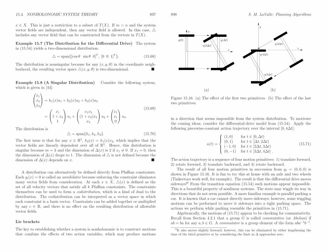
15.4. NONHOLONOMIC SYSTEM THEORY 897
x ∈ X. This is just a restriction to a subset of T (X). If m = n and the systemvector fields are independent, then any vector field is allowed. In this case, △includes any vector field that can be constructed from the vectors in T (X).
Example 15.7 (The Distribution for the Differential Drive) The systemin (15.54) yields a two-dimensional distribution:
△ = span{[cos θ sin θ 0]T , [0 0 1]T}. (15.68)
The distribution is nonsingular because for any (x, y, θ) in the coordinate neigh-borhood, the resulting vector space △(x, y, θ) is two-dimensional. �
Example 15.8 (A Singular Distribution) Consider the following system,which is given in [44]:
x1
x2
x3
= h1(x)u1 + h2(x)u2 + h3(x)u3
=
x1
1 + x3
1
u1 +
x1x2
(1 + x3)x2
x2
u2 +
x1
x1
0
u3.
(15.69)
The distribution is△ = span{h1, h2, h3}. (15.70)
The first issue is that for any x ∈ R3, h2(x) = h1(x)x2, which implies that the
vector fields are linearly dependent over all of R3. Hence, this distribution is
singular because m = 3 and the dimension of ∆(x) is 2 if x1 6= 0. If x1 = 0, thenthe dimension of ∆(x) drops to 1. The dimension of △ is not defined because thedimension of ∆(x) depends on x. �
A distribution can alternatively be defined directly from Pfaffian constraints.Each gi(x) = 0 is called an annihilator because enforcing the constraint eliminatesmany vector fields from consideration. At each x ∈ X, △(x) is defined as theset of all velocity vectors that satisfy all k Pfaffian constraints. The constraintsthemselves can be used to form a codistribution, which is a kind of dual to thedistribution. The codistribution can be interpreted as a vector space in whicheach constraint is a basis vector. Constraints can be added together or multipliedby any c ∈ R, and there is no effect on the resulting distribution of allowablevector fields.
Lie brackets
The key to establishing whether a system is nonholonomic is to construct motionsthat combine the effects of two action variables, which may produce motions
898 S. M. LaValle: Planning Algorithms
q(0) q(∆t)
q(2∆t)
x
y
q(2∆t)
q(4∆t)
q(3∆t)
y
x
(a) (b)
Figure 15.16: (a) The effect of the first two primitives. (b) The effect of the lasttwo primitives.
in a direction that seems impossible from the system distribution. To motivatethe coming ideas, consider the differential-drive model from (15.54). Apply thefollowing piecewise-constant action trajectory over the interval [0, 4∆t]:
u(t) =
(1, 0) for t ∈ [0,∆t)(0, 1) for t ∈ [∆t, 2∆t)(−1, 0) for t ∈ [2∆t, 3∆t)(0,−1) for t ∈ [3∆t, 4∆t] .
(15.71)
The action trajectory is a sequence of four motion primitives: 1) translate forward,2) rotate forward, 3) translate backward, and 4) rotate backward.
The result of all four motion primitives in succession from qI = (0, 0, 0) isshown in Figure 15.16. It is fun to try this at home with an axle and two wheels(Tinkertoys work well, for example). The result is that the differential drive movessideways!9 From the transition equation (15.54) such motions appear impossible.This is a beautiful property of nonlinear systems. The state may wiggle its way indirections that do not seem possible. A more familiar example is parallel parking acar. It is known that a car cannot directly move sideways; however, some wigglingmotions can be performed to move it sideways into a tight parking space. Theactions we perform while parking resemble the primitives in (15.71).
Algebraically, the motions of (15.71) appear to be checking for commutativity.Recall from Section 4.2.1 that a group G is called commutative (or Abelian) ifab = ba for any a, b ∈ G. A commutator is a group element of the form aba−1b−1.
9It also moves slightly forward; however, this can be eliminated by either lengthening thetime of the third primitive or by considering the limit as ∆ approaches zero.

15.4. NONHOLONOMIC SYSTEM THEORY 899
−g
−f
g
fx(∆t)
x(2∆t)
x(0)
x(3∆t)
Figure 15.17: The velocity obtained by the Lie bracket can be approximated bya sequence of four motion primitives.
If the group is commutative, then aba−1b−1 = e (the identity element) for anya, b ∈ G. If a nonidentity element of G is produced by the commutator, then thegroup is not commutative. Similarly, if the trajectory arising from (15.71) does notform a loop (by returning to the starting point), then the motion primitives do notcommute. Therefore, a sequence of motion primitives in (15.71) will be referred toas the commutator motion. It will turn out that if the commutator motion cannotproduce any velocities not allowed by the system distribution, then the system iscompletely integrable. This means that if we are trapped on a surface, then it isimpossible to leave the surface by using commutator motions.
Now generalize the differential drive to any driftless control-affine system thathas two action variables:
x = f(x)u1 + g(x)u2. (15.72)
Using the notation of (15.53), the vector fields would be h1 and h2; however, fand g are chosen here to allow subscripts to denote the components of the vectorfield in the coming explanation.
Suppose that the commutator motion (15.71) is applied to (15.72) as shown inFigure 15.17. Determining the resulting motion requires some general computa-tions, as opposed to the simple geometric arguments that could be made for thedifferential drive. If would be convenient to have an expression for the velocityobtained in the limit as ∆t approaches zero. This can be obtained by using Tay-lor series arguments. These are simplified by the fact that the action history ispiecewise constant.
The coming derivation will require an expression for x under the application ofa constant action. For each action, a vector field of the form x = h(x) is obtained.Upon differentiation, this yields
x =dh
dt=
∂h
∂x
dx
dt=
∂h
dxx =
∂h
dxh(x). (15.73)
This follows from the chain rule because h is a function of x, which itself is a
900 S. M. LaValle: Planning Algorithms
function of t. The derivative ∂h/∂x is actually an n× n Jacobian matrix, whichis multiplied by the vector x. To further clarify (15.73), each component can beexpressed as
xi =d
dthi(x(t)) =
n∑
j=1
∂hi∂xj
hj. (15.74)
Now the state trajectory under the application of (15.71) will be determinedusing the Taylor series, which was given in (14.17). The state trajectory thatresults from the first motion primitive u = (1, 0) can be expressed as
x(∆t) = x(0) + ∆t x(0) + 12(∆t)2 x(0) + · · ·
= x(0) + ∆t f(x(0)) +1
2(∆t)2
∂f
∂x
∣
∣
∣
x(0)f(x(0)) + · · · ,
(15.75)
which makes use of (15.73) in the second line. The Taylor series expansion for thesecond primitive is
x(2∆t) = x(∆t) + ∆t g(x(∆t)) +1
2(∆t)2
∂g
∂x
∣
∣
∣
x(∆t)g(x(∆t)) + · · · . (15.76)
An expression for g(x(∆t)) can be obtained by using the Taylor series expansionin (15.75) to express x(∆t). The first terms after substitution and simplificationare
x(2∆t) = x(0) + ∆t (f + g) + (∆t)2(
1
2
∂f
∂xf +
∂g
∂xf +
1
2
∂g
∂xg
)
+ · · · . (15.77)
To simplify the expression, the evaluation at x(0) has been dropped from everyoccurrence of f and g and their derivatives.
The idea of substituting previous Taylor series expansions as they are neededcan be repeated for the remaining two motion primitives. The Taylor series ex-pansion for the result after the third primitive is
x(3∆t) = x(0) + ∆t g + (∆t)2(
∂g
∂xf −
∂f
∂xg +
1
2
∂g
∂xg
)
+ · · · . (15.78)
Finally, the Taylor series expansion after all four primitives have been applied is
x(4∆t) = x(0) + (∆t)2(
∂g
∂xf −
∂f
∂xg
)
+ · · · . (15.79)
Taking the limit yields
lim∆t→0
x(4∆t)− x(0)
(∆t)2=
∂g
∂xf −
∂f
∂xg, (15.80)

15.4. NONHOLONOMIC SYSTEM THEORY 901
which is called the Lie bracket of f and g and is denoted by [f, g]. Similar to(15.74), the ith component can be expressed as
[f, g]i =n∑
j=1
(
fj∂gi∂xj
− gj∂fi∂xj
)
. (15.81)
The Lie bracket is an important operation in many subjects, and is related to thePoisson and Jacobi brackets that arise in physics and mathematics.
Example 15.9 (Lie Bracket for the Differential Drive) The Lie bracket shouldindicate that sideways motions are possible for the differential drive. Consider tak-ing the Lie bracket of the two vector fields used in (15.54). Let f = [cos θ sin θ 0]T
and g = [0 0 1]T . Rename h1 and h2 to f and g to allow subscripts to denotethe components of a vector field.
By applying (15.81), the Lie bracket [f, g] is
[f, g]1 = f1∂g1∂x
− g1∂f1∂x
+ f2∂g1∂y
− g2∂f1∂y
+ f3∂g1∂θ
− g3∂f1∂θ
= sin θ
[f, g]2 = f1∂g2∂x
− g1∂f2∂x
+ f2∂g2∂y
− g2∂f2∂y
+ f3∂g2∂θ
− g3∂f2∂θ
= − cos θ
[f, g]3 = f1∂g3∂x
− g1∂f3∂x
+ f2∂g3∂y
− g2∂f3∂y
+ f3∂g3∂θ
− g3∂f3∂θ
= 0.
(15.82)
The resulting vector field is [f, g] = [sin θ − cos θ 0]T , which indicates the side-ways motion, as desired. When evaluated at q = (0, 0, 0), the vector [0 − 1 0]T
is obtained. This means that performing short commutator motions wiggles thedifferential drive sideways in the −y direction, which we already knew from Figure15.16. �
Example 15.10 (Lie Bracket of Linear Vector Fields) Suppose that eachvector field is a linear function of x. The n × n Jacobians ∂f/∂x and ∂g/∂x areconstant.
As a simple example, recall the nonholonomic integrator (13.43). In the linear-algebra form, the system is
x1
x2
x3
=
10
−x2
u1 +
01x1
u2. (15.83)
Let f = h1 and g = h2. The Jacobian matrices are
∂f
∂x=
0 0 00 0 00 −1 0
and∂g
∂x=
0 0 00 0 01 0 0
. (15.84)
902 S. M. LaValle: Planning Algorithms
Using (15.80),
∂g
∂xf −
∂f
∂xg =
0 0 00 0 01 0 0
10
−x2
−
0 0 00 0 00 −1 0
01
−x1
=
002
. (15.85)
This result can be verified using (15.81).�
The Frobenius Theorem
The Lie bracket is the only tool needed to determine whether a system is com-pletely integrable (holonomic) or nonholonomic (not integrable). Suppose that asystem of the form (15.53) is given. Using the m system vector fields h1, . . ., hmthere are (m2 ) Lie brackets of the form [hi, hj] for i < j that can be formed. Adistribution △ is called involutive [17] if for each of these brackets there exist mcoefficients ck ∈ R such that
[hi, hj ] =m∑
k=1
ckhk. (15.86)
In other words, every Lie bracket can be expressed as a linear combination of thesystem vector fields, and therefore it already belongs to △. The Lie brackets areunable to escape △ and generate new directions of motion. We did not need toconsider all n2 possible Lie brackets of the system vector fields because it turnsout that [hi, hj] = −[hj, hi] and consequently [hi, hi] = 0. Therefore, the definitionof involutive is not altered by looking only at the (m2 ) pairs.
If the system is smooth and the distribution is nonsingular, then the Frobeniustheorem immediately characterizes integrability:
A system is completely integrable if and only if it is involutive.
Proofs of the Frobenius theorem appear in numerous differential geometry andcontrol theory books [17, 23, 44, 75]. There also exist versions that do not requirethe distribution to be nonsingular.
Determining integrability involves performing Lie brackets and determiningwhether (15.86) is satisfied. The search for the coefficients can luckily be avoidedby using linear algebra tests for linear independence. The n × m matrix H(x),which was defined in (15.56), can be augmented into an n× (m+1) matrix H ′(x)by adding [hi, hj] as a new column. If the rank of H ′(x) is m + 1 for any pairhi and hj, then it is immediately known that the system is nonholonomic. If therank of H ′(x) is m for all Lie brackets, then the system is completely integrable.Driftless linear systems, which are expressed as x = Bu for a fixed matrix B, arecompletely integrable because all Lie brackets are zero.

15.4. NONHOLONOMIC SYSTEM THEORY 903
Example 15.11 (The Differential Drive Is Nonholonomic) For the dif-ferential drive model in (15.54), the Lie bracket [f, g] was determined in Example15.9 to be [sin θ − cos θ 0]T . The matrix H ′(q), in which q = (x, y, θ), is
H ′(q) =
cos θ 0 sin θsin θ 0 − cos θ0 1 0
. (15.87)
The rank of H ′(q) is 3 for all q ∈ C (the determinant of H ′(q) is 1). Therefore, bythe Frobenius theorem, the system is nonholonomic. �
Example 15.12 (The Nonholonomic Integrator Is Nonholonomic) Wewould hope that the nonholonomic integrator is nonholonomic. In Example 15.10,the Lie bracket was determined to be [0 0 2]T . The matrix H ′(q) is
H ′(q) =
1 0 00 1 0
−x2 x1 2
, (15.88)
which clearly has full rank for all q ∈ C. �
Example 15.13 (Trapped on a Sphere) Suppose that the following systemis given:
x1
x2
x3
=
x2
−x1
0
u1 +
x3
0−x1
u2, (15.89)
for which X = R3 and U = R
2. Since the vector fields are linear, the Jacobiansare constant (as in Example 15.10):
∂f
∂x=
0 1 0−1 0 00 0 0
and∂g
∂x=
0 0 10 0 0−1 0 0
. (15.90)
Using (15.80),
∂g
∂xf −
∂f
∂xg =
0 0 10 0 0−1 0 0
x2−x10
−
0 1 0−1 0 00 0 0
x30
−x1
=
0x3−x2
. (15.91)
This yields the matrix
H ′(x) =
x2 −x1 0x3 0 −x1
0 x3 −x2
. (15.92)
904 S. M. LaValle: Planning Algorithms
The determinant is zero for all x ∈ R3, which means that [f, g] is never linearly
independent of f and g. Therefore, the system is completely integrable.10
The system can actually be constructed by differentiating the equation of asphere. Let
f(x) = x21 + x2
2 + x23 − r2 = 0, (15.93)
and differentiate with respect to time to obtain
x1x1 + x2x2 + x3x3 = 0, (15.94)
which is a Pfaffian constraint. A parametric representation of the set of vectorsthat satisfy (15.94) is given by (15.89). For each (u1, u2) ∈ R
2, (15.89) yieldsa vector that satisfies (15.94). Thus, this was an example of being trapped ona sphere, which we would expect to be completely integrable. It was difficult,however, to suspect this using only (15.89). �
15.4.3 Determining Controllability
Determining complete integrability is the first step toward determining whethera driftless control-affine system is STLC. The Lie bracket attempts to producemotions in directions that do not seem to be allowed by the system distribution.At each q, a velocity not in △(q) may be produced by the Lie bracket. Byworking further with Lie brackets, it is possible to completely characterize all ofthe directions that are possible from each q. So far, the Lie brackets have only beenapplied to the system vector fields h1, . . ., hm. It is possible to proceed further byapplying Lie bracket operations on Lie brackets. For example, [h1, [h1, h2]] can becomputed. This might generate a vector field that is linearly independent of allof the vector fields considered in Section 15.4.2 for the Frobenius theorem. Themain idea in this section is to apply the Lie bracket recursively until no moreindependent vector fields can be found. The result is called the Lie algebra. Ifthe number of independent vector fields obtained in this way is the dimension ofX, then it turns out that the system is STLC.
The Lie algebra
The notion of a Lie algebra is first established in general. Let V be any vectorspace with coefficients in R. In V , the vectors can be added or multiplied byelements of R; however, there is no way to “multiply” two vectors to obtain athird. The Lie algebra introduces a product operation to V . The product iscalled a bracket or Lie bracket (considered here as a generalization of the previousLie bracket) and is denoted by [·, ·] : V × V → V .
10This system is singular at the origin. A variant of the Frobenius theorem given here istechnically needed.

15.4. NONHOLONOMIC SYSTEM THEORY 905
To be a Lie algebra obtained from V , the bracket must satisfy the followingthree axioms:
1. Bilinearity: For any a, b ∈ R and u, v, w ∈ V ,
[au+ bv, w] = a[u, w] + b[v, w]
[u, av + bw] = a[u, w] + b[u, w].(15.95)
2. Skew symmetry: For any u, v ∈ V ,
[u, v] = −[v, u]. (15.96)
This means that the bracket is anti-commutative.
3. Jacobi identity: For any u, v, w ∈ V ,
[[u, v], w] + [[v, w], u] + [[w, u], v] = 0. (15.97)
Note that the bracket is not even associative.
Let L(V ) denote the Lie algebra of V . This is a vector space that includes allelements of V and any new elements that can be obtained via Lie bracket opera-tions. The Lie algebra L(V ) includes every vector that can be obtained from anyfinite number of nested Lie bracket operations. Thus, describing a Lie algebrarequires characterizing all vectors that are obtained under the algebraic closure ofthe bracket operation. Since L(V ) is a vector space, this is accomplished by find-ing a basis of independent vectors of which all elements of L(V ) can be expressedas a linear combination.
Example 15.14 (The Vector Cross Product) Let V be the vector spaceover R3 that is used in vector calculus. The basis elements are often denoted ası, , and k. A bracket for this vector space is simply the cross product
[u, v] = u× v. (15.98)
It can be verified that the required axioms of a Lie bracket are satisfied.One interesting property of the cross product that is exploited often in analytic
geometry is that it produces a vector outside of the span of u and v. For example,let W be the two-dimensional subspace of vectors
W = span{ı, }. (15.99)
The cross product always yields a vector that is a multiple of k, which lies outsideof V if the product is nonzero. This behavior is very similar to constructing vectorfields that lie outside of △ using the Lie bracket in Section 15.4.2. �
906 S. M. LaValle: Planning Algorithms
Example 15.15 (Lie Algebra on Lie Groups) Lie groups are the most im-portant application of the Lie algebra concepts. Recall from Section 4.2.1 thenotion of a matrix group. Important examples throughout this book have beenSO(n) and SE(n). If interpreted as a smooth manifold, these matrix groups areexamples of Lie groups [7]. In general, a Lie group G is both a differentiablemanifold and a group with respect to some operation ◦ if and only if:
1. The product a ◦ b, interpreted as a function from G×G → G, is smooth.
2. The inverse a−1, interpreted as a function from G to G, is smooth.
The two conditions are needed to prevent the group from destroying the niceproperties that come with the smooth manifold. An important result in the studyof Lie groups is that all compact finite-dimensional Lie groups can be representedas matrix groups.
For any Lie group, a Lie algebra can be defined on a special set of vectorfields. These are defined using the left translation mapping Lg : x 7→ gx. Thevector field formed from the differential of Lg is called a left-invariant vector field.A Lie algebra can be defined on the set of these fields. The Lie bracket definitiondepends on the particular group. For the case of GL(n), the Lie bracket is
[A,B] = AB − BA. (15.100)
In this case, the Lie bracket clearly appears to be a test for commutativity. Ifthe matrices commute with respect to multiplication, then the Lie bracket is zero.The Lie brackets for SO(n) and SE(n) are given in many texts on mechanics andcontrol [23, 75]. The Lie algebra of left-invariant vector fields is an importantstructure in the study of nonlinear systems and mechanics. �
Lie algebra of the system distribution
Now suppose that a set h1, . . ., hm of vector fields is given as a driftless control-affine system, as in (15.53). Its associated distribution △ is interpreted as a vectorspace with coefficients in R, and the Lie bracket operation was given by (15.81).It can be verified that the Lie bracket operation in (15.81) satisfies the requiredaxioms for a Lie algebra.
As observed in Examples 15.9 and 15.10, the Lie bracket may produce vectorfields outside of △. By defining the Lie algebra of △ to be all vector fields that canbe obtained by applying Lie bracket operations, a potentially larger distributionL(△) is obtained. The Lie algebra can be expressed using the span notation byincluding h1, . . ., hm and all independent vector fields generated by Lie brackets.Note that no more than n independent vector fields can possibly be produced.
Example 15.16 (The Lie Algebra of the Differential Drive) The Lie al-gebra of the differential drive (15.54) is
L(△) = span{[cos θ sin θ 0]T , [0 0 1]T , [sin θ − cos θ 0]T}. (15.101)

15.4. NONHOLONOMIC SYSTEM THEORY 907
This uses the Lie bracket that was computed in (15.82) to obtain a three-dimensionalLie algebra. No further Lie brackets are needed because the maximum number ofindependent vector fields has been already obtained. �
Example 15.17 (A Lie Algebra That Involves Nested Brackets) The pre-vious example was not very interesting because the Lie algebra was generated aftercomputing only one bracket. Suppose that X = R
5 and U = R2. In this case,
there is room to obtain up to three additional, linearly independent vector fields.The dimension of the Lie algebra may be any integer from 2 to 5.
Let the system be
x1
x2
x3
x4
x5
=
10x2
x3
x4
u1 +
01000
u2. (15.102)
This is a chained-form system, which is a concept that becomes important inSection 15.5.2.
The first Lie bracket produces
[h1, h2] = [0 0 − 1 0 0]T . (15.103)
Other vector fields that can be obtained by Lie brackets are
[h1, [h1, h2]] = [0 0 0 1 0]T (15.104)
and[h1, [h1, [h1, h2]]] = [0 0 0 0 1]T . (15.105)
The resulting five vector fields are independent over all x ∈ R5. This includes
h1, h2, and the three obtained from Lie bracket operations. Independence can beestablished by placing them into a 5× 5 matrix,
1 0 0 0 00 1 0 0 0x2 0 −1 0 0x3 0 0 1 0x4 0 0 0 1
, (15.106)
which has full rank for all x ∈ R5. No additional vector fields can possibly be
independent. Therefore, the five-dimensional Lie algebra is
L(△) = span{h1, h2, [h1, h2], [h1, [h1, h2]], [h1, [h1, [h1, h2]]]}. (15.107)
�
908 S. M. LaValle: Planning Algorithms
Philip Hall basis of a Lie algebra
Determining the basis of a Lie algebra may be a long and tedious process. Thecombinations of Lie brackets in Example 15.17 were given; however, it is not knownin advance which ones will produce independent vector fields. Numerous Liebrackets may be needed, including some that are nested, such as [[h1, h2], h3]. Themaximum depth of nested Lie bracket operations is not known a priori. Therefore,a systematic search must be performed (this can in fact be modeled as a discreteplanning problem) by starting with h1, . . ., hm and iteratively generating new,independent vector fields using Lie brackets.
One popular approach is to generate the Philip Hall basis (or P. Hall basis) ofthe Lie algebra L(△). The construction of the basis essentially follows breadth-first search, in which the search depth is defined to be the number of nested levelsof bracket operations. The order (or depth) d of a Lie product is defined recursivelyas follows. For the base case, let d(hi) = 1 for any of the system vector fields. Forany Lie product [φ1, φ2], let
d([φ1, φ2]) = d(φ1) + d(φ2). (15.108)
Thus, the order is just the nesting depth (plus one) of the Lie bracket operations.For example, d([h1, h2]) = 2 and d([h1, [h2, h3]]) = 3.
In addition to standard breadth-first search, pruning should be automaticallyperformed to ensure that the skew symmetry and Jacobi identities are alwaysutilized to eliminate redundancy. A P. Hall basis is a sequence, PH = (φ1, φ2,. . .), of Lie products for which:
1. The system vector fields hi are the first m elements of PH.
2. If d(φi) < d(φj), then i < j.
3. Each [φi, φj] ∈ PH if and only if: a) φi, φj ∈ PH and i < j, and b) eitherφj = hi for some i or φj = [φl, φr] for some φl, φr ∈ PH such that l ≤ i.
It is shown in many algebra books (e.g., [78]) that this procedure results in abasis for the Lie algebra L(△). Various algorithms for computing the basis areevaluated in [33].
Example 15.18 (P. Hall Basis Up to Depth Three) The P. Hall basis sortsthe Lie products into the following sequence, which is obtained up to depth d = 3:
h1, h2, h3,[h1, h2], [h2, h3], [h1, h3],[h1, [h1, h2]], [h1, [h1, h3]], [h2, [h1, h2]], [h2, [h1, h3]],[h2, [h2, h3]], [h3, [h1, h2]], [h3, [h1, h3]], [h3, [h2, h3]] .
So far, the only Lie product eliminated by the Jacobi identity is [h1, [h2, h3]] be-cause
[h1, [h2, h3]] = [h2, [h1, h3]]− [h3, [h1, h2]]. (15.109)

15.4. NONHOLONOMIC SYSTEM THEORY 909
Note that all of the Lie products given here may not be linearly independent vec-tor fields. For a particular system, linear independence tests should be performedto delete any linearly dependent vector fields from the basis. �
When does the sequence PH terminate? Recall that dim(L(△)) can be nogreater than n, because Lx(△) ⊆ Tx(X). In other words, at every state x ∈ X,the number of possible independent velocity vectors is no more than the dimensionof the tangent space at x. Therefore, PH can be terminated once n independentvector fields are obtained because there is no possibility of finding more. Forsome systems, there may be a depth k after which all Lie brackets are zero. Suchsystems are called nilpotent of order k. This occurs, for example, if all componentsof all vector fields are polynomials. If the system is not nilpotent, then achievingtermination may be difficult. It may be the case that dim(L(△)) is strictly lessthan n, but this is usually not known in advance. It is difficult to determinewhether more Lie brackets are needed to increase the dimension or the limit hasalready been reached.
Controllability of driftless systems
The controllability of a driftless control-affine system (15.53) can be characterizedusing the Lie algebra rank condition (or LARC). Recall the definition of STLCfrom Section 15.1.3. Assume that either U = R
m or U at least contains an openset that contains the origin of Rm. The Chow-Rashevskii theorem [13, 23, 75]states:
A driftless control-affine system, (15.53), is small-time locally controllable (STLC)at a point x ∈ X if and only if dim(Lx(△)) = n, the dimension of X.
If the condition holds for every x ∈ X, then the whole system is STLC.Integrability can also be expressed in terms of dim(L(△)). Assume as usual thatm < n. The three cases are:
1. dim(L(△)) = m the system is completely integrable;2. m < dim(L(△)) < n the system is nonholonomic, but not STLC;3. dim(L(△)) = n the system is nonholonomic and STLC.
(15.110)
Example 15.19 (Controllability Examples) The differential drive, nonholo-nomic integrator, and the system from Example 15.17 are all STLC by the Chow-Rashevskii theorem because dim(L(△)) = n. This implies that the state can bechanged in any direction, even though there are differential constraints. The statecan be made to follow arbitrarily close to any smooth curve in X. A methodthat achieves this based on the Lie algebra is given in Section 15.5.1. The factthat these systems are STLC assures the existence of an LPM that satisfies the
910 S. M. LaValle: Planning Algorithms
topological property of Section 14.6.2. �
Handling Control-Affine Systems with Drift
Determining whether a system with drift (15.52), is STLC is substantially moredifficult. Imagine a mechanical system, such as a hovercraft, that is moving ata high speed. Due to momentum, it is impossible from most states to move incertain directions during an arbitrarily small interval of time. One can, however,ask whether a system is STLC from a state x ∈ X for which h0(x) = 0. Fora mechanical system, this usually means that it starts at rest. If a system withdrift is STLC, this intuitively means that it can move in any direction by hoveringaround states that are close to zero velocity for the mechanical system.
The Lie algebra techniques can be extended to determine controllability forsystems with drift; however, the tools needed are far more complicated. SeeChapter 7 of [23] for more complete coverage. Even if dim(L(△)) = n, it does notnecessarily imply that the system is STLC. It does at least imply that the systemis accessible, which motivates the definition given in Section 15.1.3. Thus, the setof achievable velocities still has dimension n; however, motions in all directionsmay not be possible due to drift. To obtain STLC, a sufficient condition is thatthe set of possible values for x contains an open set that contains the origin.
The following example clearly illustrates the main difficultly with establishingwhether a system with drift is STLC.
Example 15.20 (Accessible, Not STLC) The following simple system clearlyillustrates the difficulty caused by drift and was considered in [68]. Let X = R
2,U = R, and the state transition equation be
x1 = u
x2 = x21.
(15.111)
This system is clearly not controllable in any sense because x2 cannot be decreased.The vector fields are h0(x) = [0 x2
1]T and h1(x) = [1 0]T . The first independent
Lie bracket is[h1, [h0, h1]] = [0 − 2]. (15.112)
The two-dimensional Lie algebra is
L(△) = span{h1, [h1, [h0, h1]]}, (15.113)
which implies that the system is accessible. It is not STLC, however, because thebracket [h1, [h0, h1]] was constructed using h0 and was combined in an unfortunateway. This bracket is indicating that changing x2 is possible; however, we alreadyknow that it is not possible to decrease x2. Thus, some of the vector fields obtainedfrom Lie brackets that involve h0 may have directional constraints. �

15.5. STEERING METHODS FOR NONHOLONOMIC SYSTEMS 911
In Example 15.20, [h1, [h0, h1]] was an example of a bad bracket [86] becauseit obstructed controllability. A method of classifying brackets as good or bad hasbeen developed, and there exist theorems that imply whether a system with driftis STLC by satisfying certain conditions on the good and bad brackets. Intuitively,there must be enough good brackets to neutralize the obstructions imposed by thebad brackets [23, 86].
15.5 Steering Methods for Nonholonomic Sys-
tems
This section briefly surveys some methods that solve the BVP for nonholonomicsystems. This can be considered as a motion planning problem under differentialconstraints but in the absence of obstacles. For linear systems, optimal controltechniques can be used, as covered in Section 15.2.2. For mechanical systems thatare fully actuated, standard control techniques such as the acceleration-basedcontrol model in (8.47) can be applied. If a mechanical system is underactuated,then it is likely to be nonholonomic. As observed in Section 15.4, it is possible togenerate motions that appear at first to be prohibited. Suppose that by the Chow-Rashevskii theorem, it is shown that a driftless system is STLC. This indicatesthat it should be possible to design an LPM that successfully connects any pairof initial and goal states. The next challenge is to find an action trajectory uthat actually causes xI to reach xG upon integration in (14.1). Many methodsin Chapter 14 could actually be used, but it is assumed that these would be tooslow. The methods in this section exploit the structure of the system (e.g, itsLie algebra) and the fact that there are no obstacles to more efficiently solve theplanning problem.
15.5.1 Using the P. Hall Basis
The steering method presented in this section is due to Lafferriere and Sussmann[52]. It is assumed here that a driftless control-affine system is given, in whichX is a Lie group, as introduced in Example 15.15. Furthermore, the system isassumed to be STLC. The steering method sketched in this section follows fromthe Lie algebra L(△). The idea is to apply piecewise-constant motion primitivesto move in directions given by the P. Hall basis. If the system is nilpotent, thenthis method reaches the goal state exactly. Otherwise, it leads to an approximatemethod that can be iterated to get arbitrarily close to the goal. Furthermore,some systems are nilpotentizable by using feedback [41].
The main idea is to start with (15.53) and construct an extended system
x =s∑
i=1
bi(x)vi, (15.114)
912 S. M. LaValle: Planning Algorithms
in which each vi is an action variable, and bi is a vector field in PH, the P. Hallbasis. For every i ≤ m, each term of (15.114) is bi(x)vi = hi(x)ui, which comesfrom the original system. For i > m, each bi represents a Lie product in PH, andvi is a fictitious action variable. It is called fictitious because the velocity givenby bi for i > m cannot necessarily be achieved by using a single action variable ofthe system. In general, s may be larger than n because at each x ∈ X a differentsubset of PH may be needed to obtain n independent vectors. Also, includingmore basis elements simplifies some of the coming computations.
Example 15.21 (Extended System for the Nonholonomic Integrator) Theextended system for the nonholonomic integrator (15.83) is
x1
x2
x3
=
10
−x2
v1 +
01x1
v2 +
002
v3. (15.115)
The first two terms correspond to the original system. The last term arises fromthe Lie bracket [h1, h2]. Only one fictitious action variable is needed because thethree P. Hall vector fields are independent at every x ∈ X.
It is straightforward to move this system along a grid-based path in R3. Mo-
tions in the x1 and x2 directions are obtained by applying v1 = u1 and v2 = u2,respectively. To move the system in the x3 direction, the commutator motionin (15.71) should be performed. This corresponds to applying v3. The steeringmethod described in this section yields a generalization of this approach. Higherdegree Lie products can be used, and motion in any direction can be achieved. �
Suppose some xI and xG are given. There are two phases to the steeringmethod:
1. Determine an action trajectory v for the extended system, for which x(0) =xI and x(tF ) = xG for some tF > 0.
2. Convert v into an action trajectory u that eliminates the fictitious variablesand uses the actual m action variables u1, . . . , um.
The first phase is straightforward. For the extended system, any velocity in thetangent space, Tx(X), can be generated. Start with any smooth path τ : [0, 1] →X such that τ(0) = xI and τ(1) = xG. The velocity τ(t) along the path τ is avelocity vector in Tτ(t)(X) that can be expressed as a linear combination of thebi(τ(t)) vectors using linear algebra. The coefficients of this combination are the vivalues. The second phase is much more complicated and will be described shortly.If the system is nilpotent, then u should bring the system precisely from xI to xG.By the way it is constructed, it will also be clear how to refine u to come as closeas desired to the trajectory produced by v.

15.5. STEERING METHODS FOR NONHOLONOMIC SYSTEMS 913
Formal calculations The second phase is solved using formal algebraic com-putations. This means that the particular vector fields, differentiation, manifolds,and so on, can be ignored. The concepts involve pure algebraic manipulation.To avoid confusion with previous definitions, the term formal will be added tomany coming definitions. Recall from Section 4.4.1 the formal definitions of thealgebra of polynomials (e.g., F[x1, . . . , xn]). Let A(y1, . . . , ym) denote the formalnoncommutative algebra11 of polynomials in the variables y1, . . ., ym. The yi hereare treated as symbols and have no other assumed properties (e.g, they are notnecessarily vector fields). When polynomials are multiplied in this algebra, nosimplifications can be made based on commutativity. The algebra can be con-verted into a Lie algebra by defining a Lie bracket. For any two polynomialsp, q ∈ A(y1, . . . , ym), define the formal Lie bracket to be [p, q] = pq − qp. Theformal Lie bracket yields an equivalence relation on the algebra; this results in aformal Lie algebra L(y1, . . . , ym) (there are many equivalent expressions for thesame elements of the algebra when the formal Lie bracket is applied). Nilpotentversions of the formal algebra and formal Lie algebra can be made by forcing allmonomials of degree k + 1 to be zero. Let these be denoted by Ak(y1, . . . , ym)and Lk(y1, . . . , ym), respectively. The P. Hall basis can be applied to obtain abasis of the formal Lie algebra. Example 15.18 actually corresponds to the basisof L3(h1, h2, h3) using formal calculations.
The exponential map The steering problem will be solved by performing cal-culations on Lk(y1, . . . , ym). The formal power series of A(y1, . . . , ym) is the set ofall linear combinations of monomials, including those that have an infinite numberof terms. Similarly, the formal Lie series of L(y1, . . . , ym) can be defined.
The formal exponential map is defined for any p ∈ A(y1, . . . , ym) as
ep = 1 + p+1
2!p2 +
1
3!p3 + · · · . (15.116)
In the nilpotent case, the formal exponential map is defined for any p ∈ Ak(y1, . . . , ym)as
ep =k∑
i=0
pi
i!. (15.117)
The formal series is truncated because all terms with exponents larger than kvanish.
A formal Lie group is constructed as
Gk(y1, . . . , ym) = {ep | p ∈ Lk(y1, . . . , ym)}. (15.118)
If the formal Lie algebra is not nilpotent, then a formal Lie group G(y1, . . . , ym)can be defined as the set of all ep, in which p is represented using a formal Lieseries.
11Intuitively, being an algebra means that polynomials can be added and multiplied; for allof the required axioms, see [42].
914 S. M. LaValle: Planning Algorithms
The following example is taken from [52]:
Example 15.22 (Formal Lie Groups) Suppose that the generators x and yare given. Some elements of the formal Lie group G(x, y) are
ex = I + x+ 12x2 + 1
6x3 + · · · , (15.119)
e[x,y] = I + [x, y] + 12[x, y]2 + · · · , (15.120)
and
ex−y+3[x,y] = I + x− y + 3[x, y] + · · · , (15.121)
in which I is the formal Lie group identity. Some elements of the formal Lie groupG2(x, y) are
ex = I + x+ 12x2, (15.122)
e[x,y] = I + [x, y], (15.123)
and
ex−y+3[x,y] = I + x− y + 3[x, y] + 12(x− y)2. (15.124)
�
To be a group, the axioms given in Section 4.2.1 must be satisfied. The identityis I, and associativity clearly follows from the series representations. Each ep
has an inverse, e−p, because epe−p = I. The only remaining axiom to satisfyis closure. This is given by the Campbell-Baker-Hausdorff-Dynkin formula (orCBHD formula), for which the first terms for any p, q ∈ G(y1, . . . , ym) are
exp(p) exp(q) = exp(p+q+ 12[p, q]+ 1
12[[p, q], q]− 1
12[[p, q], p]+ 1
24[p, [q, [p, q]]]+ · · · ),
(15.125)in which exp(x) alternatively denotes ex for any x. The formula also applies toGk(y1, . . . , ym), but it becomes truncated into a finite series. This fact will beutilized later. Note that epeq 6= ep+q, which differs from the standard definition ofexponentiation.
The CBHD formula is often expressed as
epeqe−p = exp
(
∞∑
i=0
Adip q
i!
)
, (15.126)
in which Ad0p q = q, and Adip q = [p,Adi−1
p q]. The operator Ad provides a compactway to express some nested Lie bracket operations. Additional terms of (15.125)can be obtained using (15.126).

15.5. STEERING METHODS FOR NONHOLONOMIC SYSTEMS 915
The Chen-Fliess series The P. Hall basis from Section 15.4.3 applies in generalto any Lie algebra. Let B1, . . ., Bs denote a P. Hall basis for the nilpotent formalLie algebra Lk(y1, . . . , ym). An important theorem in the study of formal Liegroups is that every S ∈ Gk(y1, . . . , ym) can be expressed in terms of the P. Hallbasis of its formal Lie algebra as
S = ezsBsezs−1Bs−1 · · · ez2B2ez1B1 , (15.127)
which is called the Chen-Fliess series. The zi are sometimes called the backwardP. Hall coordinates of S (there is a forward version, for which the terms in (15.127)go from 1 to s, instead of s to 1).
Returning to the system vector fields Now the formal algebra concepts canbe applied to the steering problem. The variables become the system vector fields:yi = hi for all i from 1 to m. For the P. Hall basis elements, each Bi becomes bi.The Lie group becomes the state space X, and the Lie algebra is the familiar Liealgebra over the vector fields, which was introduced in Section 15.4.3. Considerhow an element of the Lie group must evolve over time. This can be expressedusing the differential equation
S(t) = S(t)(v1b1 + v2b2 + · · ·+ vsbs), (15.128)
which is initialized with S(0) = I. Here, S can be interpreted as a matrix, whichmay, for example, belong to SE(3).
The solution at every time t > 0 can be written using the Chen-Fliess series,(15.127):
S(t) = ezs(t)bsezs−1(t)bs−1 · · · ez2(t)b2ez1(t)b1 . (15.129)
This indicates that S(t) can be obtained by integrating b1 for time z1(t), followedby b2 for time z2(t), and so on until bs is integrated for time zs(t). Note thatthe backward P. Hall coordinates now vary over time. If we determine how theyevolve over time, then the differential equation in (15.128) is solved.
The next step is to figure out how the backward P. Hall coordinates evolve.Differentiating (15.129) with respect to time yields
S(t) =s∑
j=1
ezsbs · · · ezj+1bj+1 zjbjezjbj · · · ez1b1 . (15.130)
The Chen-Fliess-Sussmann equation There are now two expressions for S,which are given by (15.128) and (15.130). By equating them, s equations of theform
s∑
j=1
pj,kzj = vk (15.131)
916 S. M. LaValle: Planning Algorithms
are obtained, in which pj,k is a polynomial in zi variables. This makes use of theseries representation for each exponential; see Example 15.23.
The evolution of the backward P. Hall coordinates is therefore given by theChen-Fliess-Sussmann (CFS) equation:
z = Q(z)v, (15.132)
in whichQ(z) is an s×smatrix, and z(0) = 0. The entries inQ(z) are polynomials;hence, it is possible to integrate the system analytically to obtain expressions forthe zi(t).
A simple example is given, which was worked out in [33]:
Example 15.23 (The CFS Equation for the Nonholonomic Integrator)The extended system for the nonholonomic integrator was given in (15.115). Thedifferential equation (15.128) for the Lie group is
S(t) = S(t)(v1b1 + v2b2 + v3b3), (15.133)
because s = 3.There are two expressions for its solution. The Chen-Fliess series (15.129)
becomesS(t) = ez3(t)b3ez2(t)b2ez1(t)b1 . (15.134)
The initial condition S(0) = I is satisfied if zi(0) = 0 for i from 1 to 3. The secondexpression for S(t) is (15.130), which in the case of the nonholonomic integratorbecomes
S(t) =z3(t)b3ez3(t)b3ez2(t)b2ez1(t)b1+
ez3(t)b3 z2(t)b2ez2(t)b2ez1(t)b1+
ez3(t)b3ez2(t)b2 z1(t)b1ez1(t)b1 .
(15.135)
Note thatS−1(t) = e−z1(t)b1e−z2(t)b2e−z3(t)b3 . (15.136)
Equating (15.133) and (15.135) yields
S−1S = v1b1 + v2b2 + v3b3 =e−z1b1e−z2b2e−z3b3 z3b3ez3b3ez2b2ez1b1+
e−z1b1e−z2b2 z2b2ez2b2ez1b1+
e−z1b1 z1b1ez1b1 ,
(15.137)
in which the time dependencies have been suppressed to shorten the expression.The formal Lie series expansions, appropriately for the exponentials, are now used.For i = 1, 2,
ezibi = (I + zibi +12z2i b
2i ) (15.138)
ande−zibi = (I − zibi −
12z2i b
2i ). (15.139)

15.5. STEERING METHODS FOR NONHOLONOMIC SYSTEMS 917
Also,
ez3b3 = (I + z3b3) (15.140)
and
e−z3b3 = (I − z3b3). (15.141)
The truncation is clearly visible in (15.140) and (15.141). The b23 terms are absentbecause b3 is a polynomial of degree two, and its square would be of degree four.
Substitution into (15.137), performing noncommutative multiplication, andapplying the Lie bracket definition yields
z1b1 + z2(b2 − z1b3) + z3b3 = v1b1 + v2b2 + v3b3. (15.142)
Equating like terms yields the Chen-Fliess-Sussmann equation
z1 = v1
z2 = v2
z3 = v3 + z1v2.
(15.143)
Recall that v is given. By integrating (15.143) from z(0) = 0, the backward P.Hall coordinate trajectory z is obtained. �
Using the original action variables Once the CFS equation has been deter-mined, the problem is almost solved. The action trajectory v was determined fromthe given state trajectory v and the backward P. Hall coordinate trajectory z isdetermined by (15.143). The only remaining problem is that the action variablesfrom vm+1 to vs are fictitious because their associated vector fields are not partof the system. They were instead obtained from Lie bracket operations. Whenthese are applied, they interfere with each other because many of them may tryto use the same ui variables from the original system at the same time.
The CBHD formula is used to determine the solution in terms of the systemaction variables u1, . . ., um. The differential equation now becomes
S(t) = S(t)(u1h1 + u2h2 + · · ·+ umhm), (15.144)
which is initialized with S(0) = I and uses the original system instead of theextended system.
When applying vector fields over time, the CBHD formula becomes
exp(tf) exp(tg) =
exp(tf + tg +t2
2[f, g] +
t3
12[[f, g], g]−
t3
12[[f, g], f ] +
t4
24[f, [g, [f, g]]] + · · · ).
(15.145)
918 S. M. LaValle: Planning Algorithms
If the system is nilpotent, then this series is truncated, and the exact effect ofsequentially combining constant motion primitives can be determined. This leadsto a procedure for determining a finite sequence of constant motion primitives thatgenerate a motion in the same direction as prescribed by the extended system andthe action trajectory v.
15.5.2 Using Sinusoidal Action Trajectories
The steering method presented in this section is based on initial work by Brockett[19] and a substantial generalization of it by Murray and Sastry [67]. The approachapplies to several classes of systems for which the growth of independent vectorfields occurs as quickly as possible. This means that when the P. Hall basisis constructed, no elements need to be removed due to linear dependency onprevious Lie products or system vector fields. For these systems, the approachapplies sinusoids of integrally related frequencies to some action variables. Thischanges some state variables while others are automatically fixed. For more detailsbeyond the presentation here, see [57, 65, 67, 75].
Steering the nonholonomic integrator
The main idea of the method can be clearly illustrated for the nonholonomicintegrator,
x1 = u1
x2 = u2
x3 = x1u2 − x2u1,
(15.146)
which was considered throughout Section 15.5.1. This case will be explained indetail, and the methods obtained by generalizing the principles will subsequentlybe stated. The presentation given here is based on [67, 75].
As was previously indicated, growing independent vector fields as quickly aspossible is important. For the nonholonomic integrator, [h1, h2], is linearly inde-pendent of h1 and h2, as observed in Example 15.12; thus, it satisfies this property.Consider steering the system from some xI = x(0) to some xG = x(1) while opti-mizing the cost functional
∫ 1
0
(
u1(t)2 + u2(t)
2)
dt. (15.147)
The problem can be solved by using the constrained Lagrangian formulation,which was given in Section 13.4.3. The first step is to eliminate the u variables.From (15.146), the cost can be expressed in terms of x1 and x2 by using x1 = u1
and x2 = u2. The third equation in (15.146) can be written as
x3 = x1x2 − x2x1 (15.148)

15.5. STEERING METHODS FOR NONHOLONOMIC SYSTEMS 919
and will be interpreted as a constraint on the Lagrangian, which is combinedusing a (scalar) Lagrange multiplier as explained in Section 13.4.3. Define theLagrangian as
L(x, x) = (x21 + x2
2) + λ(
x3 − x1x2 + x2x1
)
, (15.149)
in which the first term comes from the integrand of (15.147), and the second termcomes from (15.148).
The Euler-Lagrange equation (13.118) yields
x1 + λx2 = 0
x2 − λx1 = 0
λ = 0.
(15.150)
Note that λ = 0 implies that λ(t) is constant for all time. To obtain a differentialequation that characterizes the optimal action trajectory, use the fact that fori = 1, 2, xi = ui and xi = ui. This yields the equations u1 = −λu2 and u2 = λu1.These can be represented as second-order linear differential equations. Based onits roots, the solution is
u1(t) = u1(0) cosλt− u2(0) sinλt
u2(t) = u1(0) sinλt+ u2(0) cosλt.(15.151)
Given initial and goal states, the optimal action trajectory is found by determiningu1(0), u2(0), and λ. Suppose that xI = x(0) = (0, 0, 0) and xG = x(1) = (0, 0, a)for some a ∈ R. Other cases can be obtained by applying transformations inSE(3) to the solution.
The state trajectories for x1 and x2 can be obtained by integration of (15.151)because ui = xi for i = 1 and i = 2. Starting from x1(0) = x2(0) = 0, this yields
x1(t) =1
λ
(
u1(0) sinλt+ u2(0) cosλt− u2(0))
x2(t) =1
λ
(
− u1(0) cosλt+ u2(0) sinλt+ u1(0))
.(15.152)
To maintain the constraint that x1(1) = x2(1) = 0, λ must be chosen as λ = 2kπfor some integer n. Integration of x3 yields
x3(t) =
∫ 1
0
(
x1u2 − x2u1
)
dt =1
λ
(
u21(0) + u2
2(0))
= a. (15.153)
The cost is∫ 1
0
(
u21(t) + u2
2(t))
dt = u21(0) + u2
2(0) = λa. (15.154)
The minimum cost is therefore achieved for k = −1, which yields λ = 2π and‖u‖ = 2πa. This fixes the magnitude of u(0), but any direction may be chosen.
The steering problem can be solved in two phases:
920 S. M. LaValle: Planning Algorithms
1. Apply any action trajectory to steer x1 and x2 to their desired values whileneglecting to consider x3.
2. Apply the solution just developed to steer x3 to the goal while x1 and x2
return to their values obtained in the first phase.
This idea can be generalized to other systems.
First-order controllable systems
The approach developed for the nonholonomic integrator generalizes to systemsof the form
xi = ui for i from 1 to m
xij = xiuj − xjui for all i, j so that i < j and 1 ≤ j ≤ m (15.155)
and
xi = ui for i from 1 to m
xij = xiuj for all i, j such that i < j and 1 ≤ j ≤ m. (15.156)
Brockett showed in [19] that for such first-order controllable systems, the optimalaction trajectory is obtained by applying a sum of sinusoids with integrally relatedfrequencies for each of the m action variables. If m is even, then the trajectory foreach variable is a sum of m/2 sinusoids at frequencies 2π, 2 · 2π, . . ., (m/2) · 2π.If m is odd, there are instead (m − 1)/2 sinusoids; the sequence of frequenciesremains the same. Suppose m is even (the odd case is similar). Each action isselected as
ui =
m/2∑
k=1
aik sin 2πkt+ bik cos 2πkt. (15.157)
The other state variables evolve as
xij = xij(0) +1
2
m/2∑
k=1
1
k(ajkbik − aikbjk), (15.158)
which provides a constraint similar to (15.153). The periodic behavior of theseaction trajectories causes the xi variables to return to their original values whilesteering the xij to their desired values. In a sense this is a vector-based general-ization in which the scalar case was the nonholonomic integrator.
Once again, a two-phase steering approach is obtained:
1. Apply any action trajectory that brings every xi to its goal value. Theevolution of the xij states is ignored in this stage.

15.5. STEERING METHODS FOR NONHOLONOMIC SYSTEMS 921
2. Apply sinusoids of integrally related frequencies to the action variables.Choose each ui(0) so that xij reaches its goal value. In this stage, thexi variables are ignored because they will return to their values obtained inthe first stage.
This method has been generalized even further to second-order controllablesystems:
xi = ui for i from 1 to m
xij = xiuj for all i, j such that i < j and 1 ≤ j ≤ m (15.159)
xijk = xijuk for all (i, j, k) ∈ J ,
in which J is the set of all unique triples formed from distinct i, j, k ∈ {1, . . . ,m}and removing unnecessary permutations due to the Jacobi identity for Lie brack-ets. For this problem, a three-phase steering method can be developed by usingideas similar to the first-order controllable case. The first phase determines xi,the second handles xij , and the third resolves xijk. See [67, 75] for more details.
Chained-form systems
Example 15.17 considered a special case of a chained-form system. The system in(15.102) can be generalized to any n as
x1 = u1 x4 = x3u1
x2 = u2... (15.160)
x3 = x2u1 xn = xn−1u1.
This can be considered as a system with higher order controllability. For thesesystems, a multi-phase approach is obtained:
1. Apply any action trajectory for u1 and u2 that brings x1 and x2 to theirgoal values. The evolution of the other states is ignored in this stage.
2. This phase is repeated for each k from 3 to n. Steer xk to its desired valueby applying
u1 = a sin 2πkt and u2 = b cos 2πkt, (15.161)
in which a and b are chosen to satisfy the constraint
xk(1) = xk(0) +( a
4π
)(k−2) b
(k − 2)!. (15.162)
Each execution of this phase causes the previous k − 1 state variables toreturn to their previous values.
922 S. M. LaValle: Planning Algorithms
For a proof of the correctness of the second phase, and more information ingeneral, see [67, 75]. It may appear that very few systems fit the forms givenin this section; however, it is sometimes possible to transform systems to fit thisform. Recall that the original simple car model in (13.15) was simplified to (15.54).Transformation methods for putting systems into chained form have been devel-oped. For systems that still cannot be put in this form, Fourier techniques canbe used to obtain approximate steering methods that are similar in spirit to themethods in this section. When the chained-form system is expressed using Pfaf-fian constraints, the result is often referred to as the Goursat normal form. Themethod can be extended even further to multi-chained-form systems.
15.5.3 Other Steering Methods
The steering methods presented so far are perhaps the most widely known; how-ever, several other alternatives exist. Most of these follow in the spirit of themethods in Sections 15.5.1 and 15.5.2 by exploiting the properties of a specificclass of systems. Some alternatives are briefly surveyed here. This is an activefield of research; it is likely that new methods will be developed in the comingyears.
Differentially flat systems Differential flatness has become an important con-cept in the development of steering methods. It was introduced by Fliess, Levine,Martin, and Rouchon in [35]; see also [66]. Intuitively, a system is said to bedifferentially flat if a set of variables called flat outputs can be found for whichall states and actions can be determined from them without integration. Thisspecifically means that for a system x = f(x, u) with X = R
n and U = Rm, there
exist flat outputs of the form
y = h(x, u, u, . . . , u(k)) (15.163)
such that there exist functions g and g′ for which
x = g(y, y, . . . , y(j)) (15.164)
andu = g′(y, y, . . . , y(j)). (15.165)
One example is the simple car pulling trailers, expressed in (13.19); the flat outputsare the position in W = R
2 of the last trailer. This property was used for motionplanning in [53]. Recent works on the steering of differentially flat systems include[53, 72, 74].
Decoupling vector fields For mechanical systems in which dynamics is con-sidered, the steering problem becomes complicated by drift. One recent approachis based on establishing that a system is kinematically controllable, which means
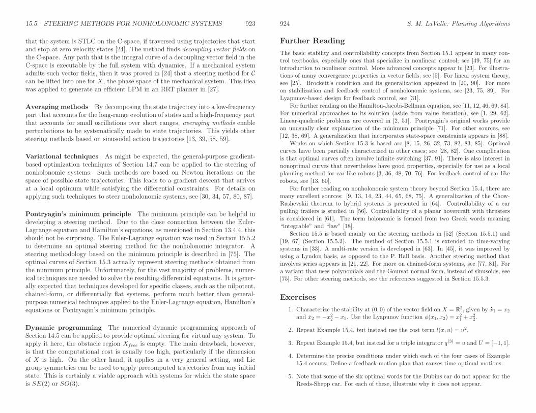
15.5. STEERING METHODS FOR NONHOLONOMIC SYSTEMS 923
that the system is STLC on the C-space, if traversed using trajectories that startand stop at zero velocity states [24]. The method finds decoupling vector fields onthe C-space. Any path that is the integral curve of a decoupling vector field in theC-space is executable by the full system with dynamics. If a mechanical systemadmits such vector fields, then it was proved in [24] that a steering method for Ccan be lifted into one for X, the phase space of the mechanical system. This ideawas applied to generate an efficient LPM in an RRT planner in [27].
Averaging methods By decomposing the state trajectory into a low-frequencypart that accounts for the long-range evolution of states and a high-frequency partthat accounts for small oscillations over short ranges, averaging methods enableperturbations to be systematically made to state trajectories. This yields othersteering methods based on sinusoidal action trajectories [13, 39, 58, 59].
Variational techniques As might be expected, the general-purpose gradient-based optimization techniques of Section 14.7 can be applied to the steering ofnonholonomic systems. Such methods are based on Newton iterations on thespace of possible state trajectories. This leads to a gradient descent that arrivesat a local optimum while satisfying the differential constraints. For details onapplying such techniques to steer nonholonomic systems, see [30, 34, 57, 80, 87].
Pontryagin’s minimum principle The minimum principle can be helpful indeveloping a steering method. Due to the close connection between the Euler-Lagrange equation and Hamilton’s equations, as mentioned in Section 13.4.4, thisshould not be surprising. The Euler-Lagrange equation was used in Section 15.5.2to determine an optimal steering method for the nonholonomic integrator. Asteering methodology based on the minimum principle is described in [75]. Theoptimal curves of Section 15.3 actually represent steering methods obtained fromthe minimum principle. Unfortunately, for the vast majority of problems, numer-ical techniques are needed to solve the resulting differential equations. It is gener-ally expected that techniques developed for specific classes, such as the nilpotent,chained-form, or differentially flat systems, perform much better than general-purpose numerical techniques applied to the Euler-Lagrange equation, Hamilton’sequations or Pontryagin’s minimum principle.
Dynamic programming The numerical dynamic programming approach ofSection 14.5 can be applied to provide optimal steering for virtual any system. Toapply it here, the obstacle region Xfree is empty. The main drawback, however,is that the computational cost is usually too high, particularly if the dimensionof X is high. On the other hand, it applies in a very general setting, and Liegroup symmetries can be used to apply precomputed trajectories from any initialstate. This is certainly a viable approach with systems for which the state spaceis SE(2) or SO(3).
924 S. M. LaValle: Planning Algorithms
Further Reading
The basic stability and controllability concepts from Section 15.1 appear in many con-trol textbooks, especially ones that specialize in nonlinear control; see [49, 75] for anintroduction to nonlinear control. More advanced concepts appear in [23]. For illustra-tions of many convergence properties in vector fields, see [5]. For linear system theory,see [25]. Brockett’s condition and its generalization appeared in [20, 90]. For moreon stabilization and feedback control of nonholonomic systems, see [23, 75, 89]. ForLyapunov-based design for feedback control, see [31].
For further reading on the Hamilton-Jacobi-Bellman equation, see [11, 12, 46, 69, 84].For numerical approaches to its solution (aside from value iteration), see [1, 29, 62].Linear-quadratic problems are covered in [2, 51]. Pontryagin’s original works providean unusually clear explanation of the minimum principle [71]. For other sources, see[12, 38, 69]. A generalization that incorporates state-space constraints appears in [88].
Works on which Section 15.3 is based are [8, 15, 26, 32, 73, 82, 83, 85]. Optimalcurves have been partially characterized in other cases; see [28, 82]. One complicationis that optimal curves often involve infinite switching [37, 91]. There is also interest innonoptimal curves that nevertheless have good properties, especially for use as a localplanning method for car-like robots [3, 36, 48, 70, 76]. For feedback control of car-likerobots, see [13, 60].
For further reading on nonholonomic system theory beyond Section 15.4, there aremany excellent sources: [9, 13, 14, 23, 44, 65, 68, 75]. A generalization of the Chow-Rashevskii theorem to hybrid systems is presented in [64]. Controllability of a carpulling trailers is studied in [56]. Controllability of a planar hovercraft with thrustersis considered in [61]. The term holonomic is formed from two Greek words meaning“integrable” and “law” [18].
Section 15.5 is based mainly on the steering methods in [52] (Section 15.5.1) and[19, 67] (Section 15.5.2). The method of Section 15.5.1 is extended to time-varyingsystems in [33]. A multi-rate version is developed in [63]. In [45], it was improved byusing a Lyndon basis, as opposed to the P. Hall basis. Another steering method thatinvolves series appears in [21, 22]. For more on chained-form systems, see [77, 81]. Fora variant that uses polynomials and the Goursat normal form, instead of sinusoids, see[75]. For other steering methods, see the references suggested in Section 15.5.3.
Exercises
1. Characterize the stability at (0, 0) of the vector field on X = R2, given by x1 = x2
and x2 = −x22 − x1. Use the Lyapunov function φ(x1, x2) = x21 + x22.
2. Repeat Example 15.4, but instead use the cost term l(x, u) = u2.
3. Repeat Example 15.4, but instead for a triple integrator q(3) = u and U = [−1, 1].
4. Determine the precise conditions under which each of the four cases of Example15.4 occurs. Define a feedback motion plan that causes time-optimal motions.
5. Note that some of the six optimal words for the Dubins car do not appear for theReeds-Shepp car. For each of these, illustrate why it does not appear.

15.5. STEERING METHODS FOR NONHOLONOMIC SYSTEMS 925
6. Retrace the steps of the Taylor series argument for deriving the Lie bracket inSection 15.4.2. Arrive at (15.81) by showing all steps in detail (smaller steps areskipped in Section 15.4.2).
7. Determine whether the following system is nonholonomic and STLC:
q1 = u1 q4 = q22u1
q2 = u2 q5 = q21u2 (15.166)
q3 = q1u2 − q2u1.
8. Prove that linear systems x = Ax+Bu for constant matrices A and B cannot benonholonomic.
9. Determine whether the following system is nonholonomic and STLC:
x
y
θ
ψ
=
cos θsin θ0
− sinψ
u1 +
0011
u2. (15.167)
10. Using the commutator motion and constant actions for the differential drive,develop a lattice over its configuration space.
11. Consider a smooth nonlinear system that has only one action variable and an n-dimensional state space for n > 1. Are such systems always completely integrable,always nonholonomic, or is either possible?
12. Generalize Example 15.17 to Rn with two action variables. Determine whether
the system is STLC for any n > 5.
13. Show that the vector cross product on R3 indeed produces a Lie algebra when
used as a bracket operation.
14. Derive the CFS equation for the following system:
q1 = u1 q3 = q1u2 − q2u1
q2 = u2 q4 = q22u1. (15.168)
Implementations
15. Implement software that computes the P. Hall basis up to any desired order (thisis only symbolic computation; the Lie brackets are not expanded).
16. Implement software that displays the appropriate optimal path for the Dubinscar, between any given qI and qG.
15.5. STEERING METHODS FOR NONHOLONOMIC SYSTEMS i
17. Apply the planning algorithm in Section 14.4.2 to numerically determine theDubins curves. Use Dijkstra’s algorithm for the search, and use a high-resolutiongrid. Can your software obtain the same set of curves as Dubins?
18. Experiment with using Dubins curves as a local planning method (LPM) andmetric in an RRT-based planning algorithm. Does using the curves improveexecution time? Do they lead to better solutions?

ii S. M. LaValle: Planning Algorithms
Bibliography
[1] R. Abgrall. Numerical discretization of the first-order Hamilton-Jacobi equa-tion on triangular meshes. Communications on Pure and Applied Mathemat-ics, 49(12):1339–1373, December 1996.
[2] B. D. Anderson and J. B. Moore. Optimal Control: Linear-Quadratic Meth-ods. Prentice-Hall, Englewood Cliffs, NJ, 1990.
[3] D. A. Anisi, J. Hamberg, and X. Hu. Nearly time-optimal paths for a groundvehicle. Journal of Control Theory and Applications, November 2003.
[4] V. I. Arnold. Mathematical Methods of Classical Mechanics, 2nd Ed.Springer-Verlag, Berlin, 1989.
[5] D. K. Arrowsmith and C. M. Place. Dynamical Systems: Differential Equa-tions, Maps, and Chaotic Behaviour. Chapman & Hall/CRC, New York,1992.
[6] T. Basar and G. J. Olsder. Dynamic Noncooperative Game Theory, 2nd Ed.Academic, London, 1995.
[7] A. Baker. Matrix Groups. Springer-Verlag, Berlin, 2002.
[8] D. J. Balkcom and M. T. Mason. Time optimal trajectories for boundedvelocity differential drive vehicles. International Journal of Robotics Research,21(3):199–217, 2002.
[9] A. Bellaiche, F. Jean, and J. J. Risler. Geometry of nonholonomic systems.In J.-P. Laumond, editor, Robot Motion Planning and Control, pages 55–92.Springer-Verlag, Berlin, 1998.
[10] R. E. Bellman. Dynamic Programming. Princeton University Press, Prince-ton, NJ, 1957.
[11] R. E. Bellman and S. E. Dreyfus. Applied Dynamic Programming. PrincetonUniversity Press, Princeton, NJ, 1962.
[12] D. P. Bertsekas. Dynamic Programming and Optimal Control, Vol. I, 2ndEd. Athena Scientific, Belmont, MA, 2001.
iii

iv BIBLIOGRAPHY
[13] A. M. Bloch. Nonholonomic Mechanics and Control. Springer-Verlag, Berlin,2003.
[14] A. M. Bloch and P. E. Crouch. Nonholonomic control systems on Riemannianmanifolds. SIAM Journal on Control & Optimization, 33:126–148, 1995.
[15] J.-D. Boissonnat, A. Cerezo, and J. Leblond. Shortest paths of boundedcurvature in the plane. Journal of Intelligent and Robotic Systems, 11:5–20,1994.
[16] V. G. Boltyanskii. Sufficient conditions for optimality and the justificationof the dynamic programming method. SIAM Journal on Control, 4:326–361,1966.
[17] W. M. Boothby. An Introduction to Differentiable Manifolds and RiemannianGeometry. Revised 2nd Ed. Academic, New York, 2003.
[18] A. V. Borisov and I .S. Mamaev. On the history of the development ofnonholonomic dynamics. Regular and Chaotic Dynamics, 7(1):43–47, 2002.
[19] R. W. Brockett. Control theory and singular Riemannian geometry. InP. A. Fuhrman, editor, New Directions in Applied Mathematics, pages 11–27.Springer-Verlag, Berlin, 1981.
[20] R. W. Brockett. Asymptotic stability and feedback stabilization. In R. W.Brockett, R. S. Millman, and H. J. Sussmann, editors, Differential GeometricControl Theory, pages 181–191. Birkhauser, Boston, MA, 1983.
[21] F. Bullo. Series expansions for the evolution of mechanical control systems.SIAM Journal on Control & Optimization, 40(1):166–190, 2001.
[22] F. Bullo. Series expansions for analytic systems linear in control. Automatica,38(9):1425–1432, September 2002.
[23] F. Bullo and A. D. Lewis. Geometric Control of Mechanical Systems.Springer-Verlag, Berlin, 2004.
[24] F. Bullo and K. M. Lynch. Kinematic controllability for decoupled trajec-tory planning in underactuated mechanical systems. IEEE Transactions onRobotics & Automation, 17(4):402–412, 2001.
[25] C.-T. Chen. Linear System Theory and Design. Holt, Rinehart, and Winston,New York, 1984.
[26] H. Chitsaz, S. M. LaValle, D. J. Balkcom, and M. T. Mason. Minimumwheel-rotation paths for differential-drive mobile robots. In Proceedings IEEEInternational Conference on Robotics and Automation, 2006.
BIBLIOGRAPHY v
[27] P. Choudhury and K. Lynch. Trajectory planning for second-order underac-tuated mechanical systems in presence of obstacles. In Proceedings Workshopon Algorithmic Foundations of Robotics, 2002.
[28] M. Chyba, H. Sussmann, H. Maurer, and G. Vossen. Underwater vehicles:The minimum time problem. In Proceedings IEEE Conference Decision &Control, The Bahamas, December 2004.
[29] M. G. Crandall and P.-L. Lions. Viscosity solutions of Hamilton-Jacobi equa-tions. Transactions of the American Mathematical Society, 277(1):1–42, 1983.
[30] A. W. Divelbiss and J. T. Wen. Nonholonomic path planning with inequalityconstraints. In Proceedings IEEE International Conference on Robotics &Automation, pages 52–57, 1994.
[31] W. E. Dixon, A. Behal, D. M. Dawson, and S. Nagarkatti. Nonlinear Controlof Engineering Systems: A Lyapunov-Based Approach. Birkhauser, Boston,MA, 2003.
[32] L. E. Dubins. On curves of minimal length with a constraint on averagecurvature, and with prescribed initial and terminal positions and tangents.American Journal of Mathematics, 79:497–516, 1957.
[33] I. Duleba. Algorithms of Motion Planning for Nonholonomic Robots. Tech-nical University of Wroclaw, Wroclaw, Poland, 1998.
[34] C. Fernandes, L. Gurvits, and Z. X. Li. A variational approach to optimalnonholonomic motion planning. In Proceedings IEEE International Confer-ence on Robotics & Automation, pages 680–685, 1991.
[35] M. Fliess, J. Levine, P. Martin, and P. Rouchon. Flatness and defect of non-linear systems: Introductory theory and examples. International Journal ofControl, 61(6):1327–1361, 1995.
[36] T. Fraichard and A. Scheuer. From Reeds and Shepp’s to continuous-curvature paths. IEEE Transactions on Robotics, 20(6):1025–1035, December2004.
[37] A. T. Fuller. Relay control systems optimized for various performance criteria.In Automatic and Remote Control (Proceedings First World Congress IFAC,Moscow, 1960), pages 510–519. Butterworths, London, 1961.
[38] L. Grune. An adaptive grid scheme for the discrete Hamilton-Jacobi-Bellmanequation. Numerische Mathematik, 75:319–337, 1997.
[39] L. Gurvits. Averaging approach to nonholonomic motion planning. In Pro-ceedings IEEE International Conference on Robotics & Automation, pages2541–2546, 1992.

vi BIBLIOGRAPHY
[40] H. Halkin. Mathematical foundation of system optimization. In G. Leitman,editor, Topics in Optimization. Academic, New York, 1967.
[41] H. Hermes, A. Lundell, and D. Sullivan. Nilpotent bases for distributionsand control systems. Journal of Differential Equations, 55(3):385–400, 1984.
[42] T. W. Hungerford. Algebra. Springer-Verlag, Berlin, 1984.
[43] R. Isaacs. Differential Games. Wiley, New York, 1965.
[44] A. Isidori. Nonlinear Control Systems, 2nd Ed. Springer-Verlag, Berlin, 1989.
[45] G. Jacob. Lyndon discretization and exact motion planning. In ProceedingsEuropean Control Conference, 1991.
[46] V. Jurdjevic. Geometric Control Theory. Cambridge University Press, Cam-bridge, U.K., 1997.
[47] R. E. Kalman, Y.-C. Ho, and K. S. Narendra. Controllability of dynamicalsystems. Contributions to Differential Equations, 1:189–213, 1963.
[48] A. Kelly and B. Nagy. Reactive nonholonomic trajectory generation viaparametric optimal control. International Journal of Robotics Research, 22(7-8):583–601, 2003.
[49] H. K. Khalil. Nonlinear Systems. Macmillan, New York, 2002.
[50] P. R. Kumar and P. Varaiya. Stochastic Systems. Prentice-Hall, EnglewoodCliffs, NJ, 1986.
[51] H. Kwakernaak and R. Sivan. Linear Optimal Control Systems. Wiley, NewYork, 1972.
[52] G. Laffierriere and H. J. Sussmann. Motion planning for controllable systemswithout drift. In Proceedings IEEE International Conference on Robotics &Automation, 1991.
[53] F. Lamiraux and J.-P. Laumond. Flatness and small-time controllability ofmultibody mobile robots: Application to motion planning. IEEE Transac-tions on Automatic Control, 45(10):1878–1881, April 2000.
[54] J. P. LaSalle. Stability theory for ordinary differential equations. Journal ofDifferential Equations, 4:57–65, 1968.
[55] J.-C. Latombe. Robot Motion Planning. Kluwer, Boston, MA, 1991.
[56] J.-P. Laumond. Controllability of a multibody mobile robot. IEEE Transac-tions on Robotics & Automation, 9(6):755–763, December 1993.
BIBLIOGRAPHY vii
[57] J.-P. Laumond, S. Sekhavat, and F. Lamiraux. Guidelines in nonholonomicmotion planning for mobile robots. In J.-P. Laumond, editor, Robot MotionPlanning and Control, pages 1–53. Springer-Verlag, Berlin, 1998.
[58] N. E. Leonard and P. S. Krishnaprasad. Averaging for attitude control andmotion planning. In Proceedings IEEE Conference Decision & Control, pages3098–3104, December 1993.
[59] N. E. Leonard and P. S. Krishnaprasad. Motion control of drift-free left-invariant systems on lie groups. IEEE Transactions on Automatic Control,40(9):1539–1554, 1995.
[60] A. De Luca, G. Oriolo, and C. Samson. Feedback control of a nonholonomiccar-like robot. In J.-P. Laumond, editor, Robot Motion Planning and Control,pages 171–253. Springer-Verlag, Berlin, 1998.
[61] K. M. Lynch. Controllability of a planar body with unilateral thrusters. IEEETransactions on Automatic Control, 44(6):1206–1211, 1999.
[62] I. Mitchell and C. J. Tomlin. Overapproximating reachable sets by Hamilton-Jacobi projections. Journal of Scientific Computation, 19(1):323–346, 2003.
[63] S. Monaco and D. Normand-Cyrot. An introduction to motion planningunder multirate digital control. In Proceedings IEEE Conference Decision &Control, pages 1780–1785, 1992.
[64] T. Murphey. Control of Multiple Model Systems. PhD thesis, CaliforniaInstitute of Technology, May 2002.
[65] R. M. Murray, Z. Li, and S. Sastry. A Mathematical Introduction to RoboticManipulation. CRC Press, Boca Raton, FL, 1994.
[66] R. M. Murray, M. Rathinam, and W. M. Sluis. Differential flatness of me-chanical control systems. In Proceedings ASME International Congress andExposition, 1995.
[67] R. M. Murray and S. Sastry. Nonholonomic motion planning: Steering usingsinusoids. IEEE Transactions on Automatic Control, 38(5):700–716, 1993.
[68] H. Nijmeijer and A. J. van der Schaft. Nonlinear Dynamical Control Systems.Springer-Verlag, Berlin, 1990.
[69] D. A. Pierre. Optimization Theory with Applications. Dover, New York, 1986.
[70] M. Pivtoraiko and A. Kelly. Generating near minimal spanning controlsets for constrained motion planning in discrete state spaces. In Proceed-ings IEEE/RSJ International Conference on Intelligent Robots and Systems,2005.

viii BIBLIOGRAPHY
[71] L. S. Pontryagin, V. G. Boltyanskii, R. V. Gamkrelidze, and E. F.Mishchenko. L. S. Pontryagin Selected Works, Volume 4: The MathematicalTheory of Optimal Processes. Gordon and Breach, Montreux, Switzerland,1986.
[72] M. Rathinam and R. M. Murray. Configuration flatness of Lagrangian sys-tems underactuated by one control. SIAM Journal of Control & Optimiza-tion, 36(1):164–179, 1998.
[73] J. A. Reeds and L. A. Shepp. Optimal paths for a car that goes both forwardsand backwards. Pacific Journal of Mathematics, 145(2):367–393, 1990.
[74] I. M. Ross and F. Fahroo. Pseudospectral methods for optimal motion plan-ning of differentially flat systems. IEEE Transactions on Automatic Control,49(8):1410–1413, 2004.
[75] S. Sastry. Nonlinear Systems: Analysis, Stability, and Control. Springer-Verlag, Berlin, 1999.
[76] A. Scheuer and T. Fraichard. Collision-free and continuous-curvature pathplanning for car-like robots. In Proceedings IEEE International Conferenceon Robotics & Automation, pages 867–873, 1997.
[77] S. Sekhavat and J.-P. Laumond. Topological property for collision-free non-holonomic motion planning: The case of sinusoidal inputs for chained-formsystems. IEEE Transactions on Robotics & Automation, 14(5):671–680, 1998.
[78] J.-P. Serre. Lie Algebras and Lie Groups. Springer-Verlag, Berlin, 1992.
[79] R. W. Sharpe. Differential Geometry. Springer-Verlag, Berlin, 1997.
[80] E. Sontag. Gradient technique for systems with no drift: A classical idearevisited. In Proceedings IEEE Conference Decision & Control, pages 2706–2711, December 1993.
[81] O. J. Sordalen. Conversion of a car with n trailers into a chained form. InProceedings IEEE International Conference on Robotics & Automation, pages1382–1387, 1993.
[82] P. Soueres and J.-D. Boissonnat. Optimal trajectories for nonholonomic mo-bile robots. In J.-P. Laumond, editor, Robot Motion Planning and Control,pages 93–169. Springer-Verlag, Berlin, 1998.
[83] P. Soueres and J.-P. Laumond. Shortest paths synthesis for a car-like robot.In IEEE Transactions on Automatic Control, pages 672–688, 1996.
[84] R. F. Stengel. Optimal Control and Estimation. Dover, New York, 1994.
BIBLIOGRAPHY ix
[85] H. Sussmann and G. Tang. Shortest paths for the Reeds-Shepp car: A workedout example of the use of geometric techniques in nonlinear optimal control.Technical Report SYNCON 91-10, Dept. of Mathematics, Rutgers University,Piscataway, NJ, 1991.
[86] H. J. Sussmann. A general theorem on local controllability. SIAM Journalon Control & Optimization, 25(1):158–194, 1987.
[87] H. J. Sussmann. A continuation method for nonholonomic path-finding prob-lems. In Proceedings IEEE Conference Decision & Control, pages 2717–2723,December 1993.
[88] H. J. Sussmann. A very non-smooth maximum principle with state con-straints. In Proceedings IEEE Conference Decision & Control, pages 917–922,December 2005.
[89] J. T. Wen. Control of nonholonomic systems. In W. S. Levine, editor, TheControl Handbook, pages 1359–1368. CRC Press, Boca Raton, FL, 1996.
[90] J. Zabczyk. Some comments on stabilizability. Applied Mathematics andOptimization, 19(1):1–9, 1989.
[91] M. I. Zelikin and V. F. Borisov. Theory of Chattering Control. Birkhauser,Boston, MA, 1994.