chapter xx1cd-rom final version

Household Sample Surveys in Developing and Transition Countries

1

Chapter XXI

Sampling error estimation for survey data

Donna Brogan Emory University

Atlanta, Georgia, United States of America

Annex (CD-ROM)

Illustrative and comparative analyses of the Burundi Immunization Survey using five sample survey software packages


2

I. Description of the Burundi sample survey

Inference population and population parameters The population of inference for this survey is women of Burundi who gave birth between Easter of 1988 (that is to say, 3 April 1988) and February/March 1989 (when the survey was fielded). The primary population parameter of interest was proportion or percentage of women who were seropositive, defined as a tetanus antitoxin titre of at least 0.01 international units per millitre (IU/ml), thus protecting their newborn against neonatal tetanus.

Sampling plan The sampling plan for the Burundi survey was a modification of the cluster sample survey methodology developed at the World Health Organization (WHO) for its Expanded Programme on Immunization (Brogan and others, 1994). The modification, as suggested by Brogan and others (1994) and described below, yields a probability sample of dwellings or housing units and hence a probability sample of women. Various sample survey methodologists, including Brogan and others (1994), have noted that the WHO cluster sample survey methodology may not provide a probability sample of dwellings or of persons (elements). A non-probability sample of dwellings or persons may result because the standard WHO procedure eliminates the listing of dwellings within a primary sampling unit (PSU) and may allow field interviewer subjectivity to influence the sampling of “next nearest” dwellings. The country of Burundi was stratified into two geographical areas, the capital Bujumbura (urban stratum) and the rest of the country (rural stratum). Although most of the country’s population was rural (96 per cent), an equal sample size of women per stratum was planned to allow comparison of urban and rural women on seropositivity. Thus, urban women were substantially oversampled. In the rural stratum the PSU was a colline (hill), an administrative geographical unit. The PSUs were listed on the sampling frame by geographical proximity. A probability sample of 30 collines was selected, using systematic probability proportional to estimated size (ppes) sampling; the size measure was total population in the colline as indicated by the 1979 national census. For each sample colline, all dwellings were identified and listed on a dwelling sampling frame. One dwelling was randomly selected from the frame. All survey-eligible women (if any) in this selected dwelling were included in the sample and interviewed. The next adjacent dwelling on the frame was selected for the sample, and all survey-eligible women were included in the sample. Next adjacent dwellings on the frame were visited until seven women were selected from the sample colline. If there was more than one survey-eligible woman in the last dwelling visited, there could be more than seven women selected per colline, since all women in each selected dwelling were selected for the sample.


3

In the urban stratum, the PSU was a quartier or avenue, subdivisions of the city’s ten zones. The PSUs were listed on the sampling frame by geographical proximity. A probability sample of 30 quartiers was selected, using systematic ppes sampling; the size measure was total population in the quartier as measured by a preliminary survey, since the most recent census data were not reliable. A sample quartier was divided into parcelles (lots), and all parcelles for the sample quartier were listed on a sampling frame. One parcelle was randomly chosen from the frame to be in the sample. All survey-eligible women within that parcelle were included in the sample. Next adjacent parcelles on the frame were chosen until seven women were selected for the sample within each sample quartier. If there was more than one survey-eligible woman in the last parcelle visited, there could be more than seven women selected per quartier, since all women in each selected parcelle were selected for the sample. Interview Women selected into the sample were asked questions about the pregnancy that had resulted in the recent birth as well as the two previous pregnancies (if applicable). Tetanus serological testing was based on a finger prick filter paper sample of blood taken at the time of interview. Seropositivity was defined as a tetanus antitoxin titre of at least 0.01 IU/ml. The survey response rate was essentially 100 per cent, an unusually high rate. No sample women refused to participate or were absent from home during the survey field time. Weighting the sample of women Given the sampling plan described above, an equal probability sample of survey-eligible women was assumed within each stratum (urban and rural). Hence, all sample women within the same stratum would have the same value for the sampling weight variable, with the value being much lower for urban women because they were oversampled. The value of the sampling weight variable W provided with the data set was the (estimated) total population of each stratum divided by the sample size of interviewed women in that stratum. The estimated total population for Bujumbura, the urban stratum, was obtained from the preliminary survey. The estimated total population for the rural stratum was obtained by subtracting the estimated Bujumbura population from the national population projected for 1989. The weighting procedure just described is commonly used in WHO/EPI coverage surveys because estimated population figures often are not available for surveyed subpopulations, for example, children in a specified age range or urban and rural women with a recent birth. As long as the subpopulation size is proportional to the total population size, in all strata, point estimates of population proportions or means (summary or average measures) will be unbiased (or nearly unbiased) using a weighting procedure that uses estimates of total population. The WHO/EPI coverage surveys typically are not interested in estimating population totals. However, in the present chapter on variance estimation methods, it is desired to illustrate the estimation of population totals in addition to population means and proportions. Using the sampling weight W provided with the data set would result in estimated population totals that are much too large. Thus, the sampling weight W was multiplied by 0.03996, yielding a revised sampling weight W2 that was used for all analyses reported here. The scaling factor 0.03996 was


4

estimated using Burundi population and fertility data located on various web sites. This scaling factor is approximate and used only to illustrate the estimation of population totals with the various software packages. Substantive results regarding population totals for survey-eligible women in Burundi in 1989 should not be concluded from the analyses in this chapter. It is important to note that point estimates of proportions and means reported in this chapter agree with previously published results with this data set (Expanded Programme on Immunization, 1996) since W2 (the revised sampling weight) is a scalar multiple of W (the sampling weight provided with the data set). Selected variables in the Burundi data set

Some of the variables in the Burundi data set are: STRA Stratum, original survey stratification variable. 1 = rural, 2 = urban. GRAPPE Cluster (PSU) within original stratum. Coded 1 through 30 within stratum. W2 Sample weight variable (revised).

The value of W2 is 959.3 for rural women and 42 for urban women. IMMUNE Tetanus antitoxin titre. 1 = seropositive, 2 = seronegative. BLOOD Indicator variable recode of IMMUNE. 1 = seropositive, 0 = seronegative. RUR_URB Coded same as STRA: 1 = rural, 2 = urban. IUML International units of antitoxin per ml (IU/ml), a continuous variable. Min = 0, Max = 20. PSTRA Pseudo-stratum. Coded 1 through 30. PPSU PSU, coded 1 or 2 within each level of PSTRA. Note that STRA and RUR_URB are coded in exactly the same way and can be used interchangeably. Also, the two variables IMMUNE and BLOOD are just recodes of each other. Describing the Burundi sample selection method to software packages The Burundi sampling plan is described by the common sampling plan WR, discussed in section B.5 of this chapter; that is to say, the ultimate cluster variance estimate (UCVE) approach is used, where the first-stage sampling fractions in both the urban and rural stratum are assumed to be small. Since the population PSUs on both the urban and rural sampling frames were ordered by geographical proximity, and since systematic ppes sampling of PSUs was used within each stratum, implicit geographical stratification is obtained within each of the urban and rural strata. Thus, the sampling plan within each of the urban and rural strata is considered to be two sample PSUs selected from each of 15 geographical pseudo-strata. Therefore, the sample design for the purpose of variance estimation, whether using Taylor series linearization or replication methods, is 30 pseudo-strata with two sample PSUs per pseudo-stratum as opposed to two strata (urban and rural) with 30 sample PSUs per stratum. The pseudo-strata description generally is preferred because it yields more efficient variance estimation by recognizing the implicit geographical stratification. Estimated standard errors for the point estimates differ slightly in this chapter from those in previously published reports because analyses reported here defined pseudo-strata for variance estimation.


5

The variable for the pseudo-stratum is named PSTRA and coded 1, 2, …, 30. The PSU variable within the pseudo-stratum is named PPSU and is coded 1, 2, within each pseudo-stratum.

II. Burundi analyses using sample survey PROCS in SAS 8.2

Example 1: The user-written program below is input into SAS. The PROC statement specifies SURVEYMEANS, a SAS sample survey procedure for the analysis of both continuous and categorical variables. The STRATA statement specifies the pseudo-stratification variable PSTRA, the CLUSTER statement specifies the PSU variable PPSU, and the WEIGHT statement specifies the sampling weight variable W2. The common sampling plan WR is assumed by SAS. The method of variance estimation is Taylor series linearization, the only method available in the SAS sample survey procedures. The VAR statement below indicates the variable to be analysed, and the CLASS statement identifies the variable as categorical. Thus, SURVEYMEANS will estimate a one-way percentage distribution for IMMUNE. Several options on the PROC statement control the output. MEAN requests estimated proportion, STDERR requests the estimated standard error of the MEAN (proportion), CLM requests a confidence interval (95 per cent is default) for the population MEAN (proportion), SUM requests the estimated population total, STD requests the estimated standard error of SUM, CLSUM requests a confidence interval for the population SUM or total, and NOBS requests the number of observations used for each calculation. /* SAS EXAMPLE 1. ESTIMATE NUMBER OF WOMEN AND PERCENTAGE OF WOMEN WHO ARE SEROPOSITIVE. */ libname input 'C:\United_Nations\BUR_V8\' ; proc surveymeans data = input.bursort3 mean stderr clm sum std clsum nobs ; strata PSTRA ; cluster PPSU ; weight w2 ; var immune ; class immune ; TITLE "Estimated seropositivity distribution"; TITLE2 "Women in Burundi with recent birth"; TITLE3 "April 1988 TO February/March 1989"; FORMAT IMMUNE PROTECTF. ; RUN ;

Estimated seropositivity distribution Women in Burundi with recent birth April 1988 to February/March 1989

The SURVEYMEANS Procedure, SAS 8.2

Data Summary

Number of Strata 30

Number of Clusters 60 Number of Observations 418 Sum of Weights 212023.6


6

The printout above indicates that the data set has 30 strata (pseudo-strata) and a total of 60 clusters or PSUs. The sample size is 418 women. The sum of the sampling weight variable W2 for the 418 sample women is 212,024, the estimated number of women in the inference population.

Class-level Information

Class Variable Label Levels Values

IMMUNE PRO_BLOOD 2 SEROPOS1 SERONEG2

The printout above identifies the categorical (CLASS) variable in the analysis and indicates the number of levels for each variable and the codes (value labels) for each variable.

Statistics

Std Error Lower 95% Variable Label N Mean of Mean CL for Mean ----------------------------------------------------------------------------------------------- IMMUNE=SEROPOS1 PRO_BLOOD 313 0.672026 0.038296 0.593815 IMMUNE=SERONEG2 105 0.327974 0.038296 0.249763 -----------------------------------------------------------------------------------------------

Statistics Upper 95% Lower 95% Upper 95% Variable CL for Mean Sum Std Dev CL for Sum CL for Sum ------------------------------------------------------------------------------------------------ IMMUNE=SEROPOS1 0.750237 142485 8848.097742 124415 160556 IMMUNE=SERONEG2 0.406185 69538 7855.577944 53495 85582 ------------------------------------------------------------------------------------------------

The above printout shows that 313 sample women were seropositive and 105 sample women were seronegative. The estimated proportion of women seropositive in the population is 0.672026, with estimated standard error of .038296. A 95 per cent confidence interval on the proportion of women in the inference population who are seropositive is (.593815, .750237). The estimated number of women in the population who are seropositive is 142,485, with estimated standard error of 8,848. A 95 per cent confidence interval on the number of women in the population who are seropositive is (124,415; 160,556). The value of Student-t used in construction of the confidence intervals is 2.0423, which is the two-sided Student-t value with 30 df for a 95 per cent confidence interval. Example 2: The user-written program below is input into SAS. Part A of this program is similar to the SURVEYMEANS program in example 1, except the added DOMAIN statement contains the variable RUR_URB. Thus, the variable IMMUNE on the VAR statement will be analysed for each domain formed by the variable RUR_URB, in other words, for rural and urban women. The options requested on the PROC statement are the same as requested in example 1.


7

In Part B of the SAS program below, SURVEYREG (linear regression) is used to compare rural and urban women in the population on the proportion who are seropositive. In SAS version 8.2, there are no sample survey procs that do chi-square tests for categorical variables or that test linear contrasts such as the difference between two proportions or two means. However, SURVEYREG can be used to estimate the difference between two domain proportions, with estimated standard error, until these sample survey capabilities are available in SAS. The dependent variable in the linear regression is defined as the indicator variable BLOOD (1 = seropositive, 0 = not seropositive). The independent variable in the linear regression is the domain variable, namely, RUR_URB. The estimated regression coefficient for RUR_URB is the estimated difference between the two domain proportions, and its estimated standard error is given. A test of the null hypothesis that the population regression coefficient is zero is equivalent to testing the null hypothesis that the two population proportions are equal. /* SAS EXAMPLE 2. ESTIMATE NUMBER OF WOMEN AND PERCENTAGE OF WOMEN WHO ARE SEROPOSITIVE, FOR EACH OF THE TWO GEOGRAPHIC STRATA (RURAL/URBAN). DETERMINE WHETHER RURAL/URBAN RESIDENCE IS STATISTICALLY INDEPENDENT OF SEROPOSITIVIY. */

libname input 'C:\United_Nations\BUR_V8\' ; /* PART A. GENERATE THE POINT ESTIMATES, BY RURAL/URBAN RESIDENCE */ proc SURVEYMEANS data = input.bursort3 mean stderr clm sum std clsum nobs ; strata PSTRA ; cluster PPSU ; weight w2 ; var immune ; class immune ; domain rur_urb ; TITLE "Estimated seropositivity distribution by rural/urban status"; TITLE2 "April 1988 to February/March 1989"; TITLE3 "Women in Burundi with recent birth"; FORMAT RUR_URB STRAF. ; FORMAT IMMUNE PROTECTF. ; RUN ; /* PART B. USE PROC SURVEYREG TO TEST THE NULL HYPOTHESIS THAT PERCENTAGE SEROPOSITIVE IS THE SAME FOR RURAL WOMEN AS FOR URBAN WOMEN IN POPULATION OF INFERENCE. USE THE INDICATOR VARIABLE BLOOD AS THE DEPENDENT VARIABLE IN SURVEYREG. */ PROC SURVEYREG DATA = INPUT.BURSORT3 ; strata PSTRA ; cluster PPSU ; weight w2 ; CLASS RUR_URB ; MODEL BLOOD = RUR_URB / SOLUTION ; TITLE "Compare rural and urban women on seropositivity"; TITLE2 " April 1988 TO February/March 1989"; TITLE3 "Women in Burundi with Recent Birth";


8

FORMAT RUR_URB STRAF. ; RUN ;

Estimated seropositivity distribution by rural/urban residence

April 1988 to February/March 1989 Women in Burundi with recent birth


Data Summary

Number of Strata 30 Number of Clusters 60 Number of Observations 418 Sum of Weights 212023.6

Class-level Information Class

Variable Label Levels Values IMMUNE PRO_BLOOD 2 SEROPOS1 SERONEG2 Statistics

Std Error Lower 95% Variable Label N Mean of Mean CL for Mean ----------------------------------------------------------------------------------------------- IMMUNE=SEROPOS1 PRO_BLOOD 313 0.672026 0.038296 0.593815 IMMUNE=SERONEG2 105 0.327974 0.038296 0.249763 -----------------------------------------------------------------------------------------------

Statistics Upper 95% Lower 95% Upper 95% Variable CL for Mean Sum Std Dev CL for Sum CL for Sum ------------------------------------------------------------------------------------------------ IMMUNE=SEROPOS1 0.750237 142485 8848.097742 124415 160556 IMMUNE=SERONEG2 0.406185 69538 7855.577944 53495 85582 -------------------------------------------------------------------------------------------------

The printout above is for the entire population and is the same as the printout for Example 1 earlier. The 95 per cent confidence intervals above use Student-t = 2.042 with 30 df. The printout for the two domains (rural and urban women) follows.


9

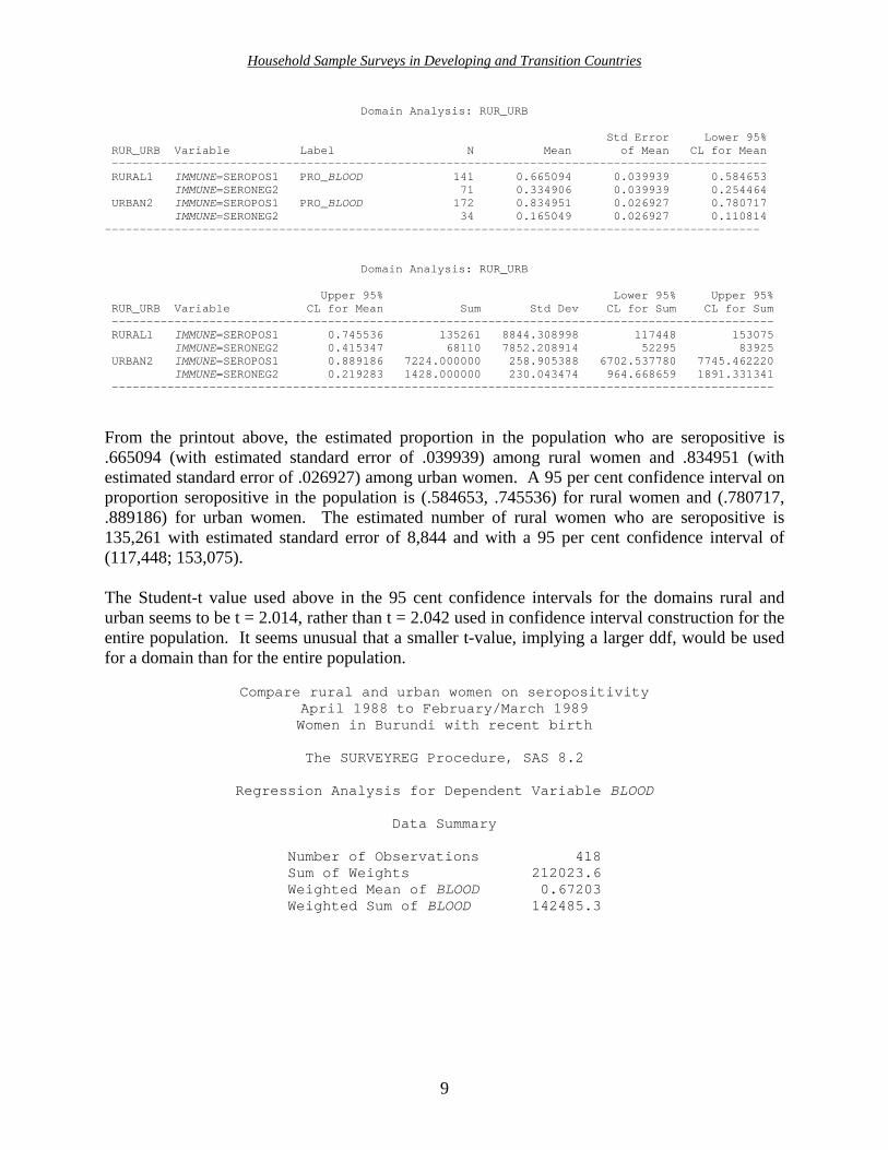
Domain Analysis: RUR_URB Std Error Lower 95% RUR_URB Variable Label N Mean of Mean CL for Mean ---------------------------------------------------------------------------------------------- RURAL1 IMMUNE=SEROPOS1 PRO_BLOOD 141 0.665094 0.039939 0.584653 IMMUNE=SERONEG2 71 0.334906 0.039939 0.254464 URBAN2 IMMUNE=SEROPOS1 PRO_BLOOD 172 0.834951 0.026927 0.780717 IMMUNE=SERONEG2 34 0.165049 0.026927 0.110814 ----------------------------------------------------------------------------------------------

Domain Analysis: RUR_URB Upper 95% Lower 95% Upper 95% RUR_URB Variable CL for Mean Sum Std Dev CL for Sum CL for Sum ----------------------------------------------------------------------------------------------- RURAL1 IMMUNE=SEROPOS1 0.745536 135261 8844.308998 117448 153075 IMMUNE=SERONEG2 0.415347 68110 7852.208914 52295 83925 URBAN2 IMMUNE=SEROPOS1 0.889186 7224.000000 258.905388 6702.537780 7745.462220 IMMUNE=SERONEG2 0.219283 1428.000000 230.043474 964.668659 1891.331341 -----------------------------------------------------------------------------------------------

From the printout above, the estimated proportion in the population who are seropositive is .665094 (with estimated standard error of .039939) among rural women and .834951 (with estimated standard error of .026927) among urban women. A 95 per cent confidence interval on proportion seropositive in the population is (.584653, .745536) for rural women and (.780717, .889186) for urban women. The estimated number of rural women who are seropositive is 135,261 with estimated standard error of 8,844 and with a 95 per cent confidence interval of (117,448; 153,075). The Student-t value used above in the 95 cent confidence intervals for the domains rural and urban seems to be t = 2.014, rather than t = 2.042 used in confidence interval construction for the entire population. It seems unusual that a smaller t-value, implying a larger ddf, would be used for a domain than for the entire population.

Compare rural and urban women on seropositivity

April 1988 to February/March 1989 Women in Burundi with recent birth

The SURVEYREG Procedure, SAS 8.2

Regression Analysis for Dependent Variable BLOOD

Data Summary

Number of Observations 418 Sum of Weights 212023.6 Weighted Mean of BLOOD 0.67203 Weighted Sum of BLOOD 142485.3


10

Note above at the beginning of the SURVEYREG output that the number of observations (women) in the data set is 418. The sum of the weight variable W2 over these 418 sample women is 212,023.6, as in example 1; this is an estimate of the number of women in the population. The weighted mean of the variable BLOOD is the estimated proportion of women in the population who are seropositive, namely, 0.67203, the same answer as in Part A of this example 2. The weighted sum of the variable BLOOD is the estimated number of women who are seropositive, namely, 142,485, and agrees with the point estimate from Part A of this example 2.

Design Summary

Number of Strata 30 Number of Clusters 60

The design summary above indicates that SAS SURVEYREG found 30 strata (pseudo-strata) and a total of 60 PSUs or clusters. Thus, the denominator degrees of freedom (ddf) stated below for the F tests and t-tests is 60 – 30 = 30.

Fit Statistics

R-square 0.005124 Root MSE 0.4694 Denominator DF 30



RUR_URB RURAL/URBAN 2 RURAL1 URBAN2

ANOVA for Dependent Variable BLOOD Sum of Mean Source DF Squares Square F Value Pr > F Model 1 239.44 239.4364 2.14 0.1440 Error 416 46492.09 111.7598 Corrected Total 417 46731.52 Tests of Model Effects Effect Num DF F Value Pr > F Model 1 12.41 0.0014 Intercept 1 967.47 <.0001 RUR_URB 1 12.41 0.0014 NOTE: The denominator degrees of freedom for the F tests is 30.


11

The F-test above for the one df variable RUR_URB (F = 12.41, p = .0014) indicates that the following null hypothesis is rejected: the population regression coefficient for the rural/urban factor is zero, in other words, the proportion of women seropositive is the same among urban women and rural women. Estimated regression eoefficients Standard Parameter Estimate error t Value Pr > |t| Intercept 0.8349515 0.02695951 30.97 <.0001 RUR_URB RURAL1 -0.1698571 0.04822641 -3.52 0.0014 RUR_URB URBAN2 0.0000000 0.00000000 . . Note: The denominator degrees of freedom for the t tests is 30. Matrix X'WX is singular and a generalized inverse was used to solve the normal equations. Estimates are not unique. From the printout to Part A earlier, the estimated proportion in the population who are seropositive is .665094 for rural women and .834951 for urban women. The difference in these estimated proportions is (.665094 - .834951) = -.169857, which is the estimated regression coefficient above for rural women compared to urban women (the reference group used by SURVEYREG). The estimated standard error of this estimated difference is .04822641. The t-statistic is defined as the estimated regression coefficient divided by its estimated standard error, in other words, (-.1698571/.04822641) = -3.52, with a p-value of .0014. The null hypothesis is that the population regression coefficient is zero; this null hypothesis is rejected. The conclusion is that rural and urban women in the inference population have a different prevalence of seropositivity, and the prevalence is lower for rural women. Note that the square root of the F-statistic 12.41 for the rural/urban independent variable is 3.52, the absolute value of the t-statistic for the rural/urban variable. The F-test and the t-test are equivalent because the rural/urban variable has 1 df. Example 3: The user-written program below is input into SAS. Part A of the program generates estimated means using SURVEYMEANS and Part B of the program compares the two estimated means using SURVEYREG. In Part A, the PROC statement instructs SURVEYMEANS to analyse the variable IUML named on the VAR statement. Since IUML does not appear on a CLASS statement, SURVEYMEANS assumes that IUML is a continuous variable and will estimate mean IUML. The DOMAIN statement indicates that mean IUML is to be estimated for all levels of the RUR_URB variable, in other words, for rural and urban women.


12

/* SAS EXAMPLE 3. ESTIMATE MEAN INTERNATIONAL UNITS OF ANTITOXIN ( IUML ), FOR INFERENCE POPULATION OF WOMEN AND BY RURAL/URBAN RESIDENCE. DETERMINE WHETHER RURAL/URBAN RESIDENCE IS RELATED TO MEAN IUML. */ /* PART A. GENERATE THE ESTIMATED MEANS */ libname input 'C:\United_Nations\BUR_V8\' ; proc SURVEYMEANS data = input.bursort3 ; strata PSTRA ; cluster PPSU ; weight w2 ; VAR IUML ; domain rur_urb ; TITLE "Estimated mean IUML, by rural/urban residence"; TITLE2 "April 1988 to February/March 1989"; TITLE3 "Women in Burundi with recent birth"; FORMAT RUR_URB STRAF. ; RUN ; In Part B, the program is called SURVEYREG, with IUML as the dependent variable. The only independent variable in the model is RUR_URB. SURVEYREG uses the higher coded value of RUR_URB as the reference group, namely, urban women. The estimated regression coefficient for RUR_URB is the estimated difference in mean IUML between rural and urban women. /* PART B. COMPARE RURAL/URBAN WOMEN ON MEAN IUML WITH SURVEYREG */ libname input 'C:\United_Nations\BUR_V8\' ; proc SURVEYREG data = input.bursort3 ; strata PSTRA ; cluster PPSU ; weight w2 ; CLASS RUR_URB ; MODEL IUML = RUR_URB / SOLUTION ; TITLE "Estimated mean difference of IUML, for rural/urban residence"; TITLE2 "April 1988 to February/March 1989"; TITLE3 "Women in Burundi with recent birth"; FORMAT RUR_URB STRAF. ; RUN ;


13

Estimated mean IUML, by rural/urban residence April 1988 to February/March 1989 Women in Burundi with recent birth


Data Summary

Number of strata 30 Number of clusters 60 Number of observations 418 Sum of weights 212023.6

Statistics

Std Error Lower 95% Upper 95% Variable N Mean of Mean CL for Mean CL for Mean ---------------------------------------------------------------------------------------- IUML 418 2.114074 0.354465 1.390160 2.837988 ----------------------------------------------------------------------------------------

From the output above, the estimated mean IUML for the inference population is 2.114074, with an estimated standard error of 0.354465. A 95 per cent confidence interval on mean IUML is (1.390160, 2.837988). The Student-t value used in the 95 per cent confidence interval above is t=2.042 with 30 df. Domain analysis: RUR_URB Std Error Lower 95% Upper 95% RUR_URB Variable N Mean of Mean CL for Mean CL for Mean --------------------------------------------------------------------------------------------- RURAL1 IUML 212 2.111002 0.369415 1.366962 2.855043 URBAN2 IUML 206 2.186273 0.235188 1.712580 2.659966 ---------------------------------------------------------------------------------------------

The above SURVEYMEANS output estimates mean IUML for the two domains of rural and urban women. The estimated mean IUML for rural women is 2.111002, with an estimated standard error of 0.369415. The estimated mean IUML for urban women is 2.186273 with an estimated standard error of 0.235188. The Student-t value used in the 95 per cent confidence interval above seems to be t = 2.014.


14

Estimated mean difference of IUML, for rural/urban residence April 1988 to February/March 1989 Women in Burundi with recent birth

The SURVEYREG Procedure, SAS 8.2

Regression Analysis for Dependent Variable IUML

Data Summary

Number of Observations 418 Sum of Weights 212023.6 Weighted Mean of IUML 2.11407 Weighted Sum of IUML 448233.6

Design Summary

Number of Strata 30 Number of Clusters 60

Fit Statistics

R-square 0.000012 Root MSE 4.3018 Denominator DF 30



RUR_URB RURAL/URBAN 2 RURAL1 URBAN2

ANOVA for dependent variable IUML Sum of Mean Source DF Squares Square F Value Pr > F Model 1 47 47.019 0.01 0.9436 Error 416 3904863 9386.691 Corrected Total 417 3904910

Tests of model effects

Effect Num DF F Value Pr > F

Model 1 0.03 0.8648 Intercept 1 96.06 <.0001 RUR_URB 1 0.03 0.8648


15

The above SURVEYREG output includes F-test (F =.03 for the entire model [less intercept] or for the one independent variable RUR_URB) and indicates that the variable rural/urban is not significantly related to mean IUML (since p = .8648).

The SURVEYREG procedure Regression Analysis for Dependent Variable IUML

NOTE: The denominator degrees of freedom for the F tests is 30. The statement above indicates that the denominator degrees of freedom (ddf) for the F tests is 30. The ddf is calculated as the number of PSUs in the sample (60) less the number of strata (pseudo-strata) in the sample (30). Estimated regression coefficients Standard Parameter Estimate error t Value Pr > |t| Intercept 2.1862728 0.23547064 9.28 <.0001 RUR_URB RURAL1 -0.0752705 0.43845417 -0.17 0.8648 RUR_URB URBAN2 0.0000000 0.00000000 . . NOTE: The denominator degrees of freedom for the t tests is 30. Matrix X'WX is singular and a generalized inverse was used to solve the normal equations. Estimates are not unique. The estimated regression coefficient above, -0.0752705, is the difference between the estimated mean IUML for rural (2.111002) and urban (2.186273) women (means from Part A of this Example 3.). The estimated standard error of the estimated regression coefficient is 0.43845417. The t-statistic is calculated as (-0.0752705/.43845417) = -0.17, with a p-value of 0.8648. The null hypothesis (population regression coefficient equals zero) is not rejected. The conclusion is that there is no evidence to support a difference between rural and urban women on mean IUML.

III. Burundi analyses using selected PROCS in SUDAAN 8.0 Example 1: The PROC statement of the input program below specifies CROSSTAB, a SUDAAN procedure for the analysis of categorical variables. The PROC statement includes DESIGN = WR to indicate the common sampling plan WR as discussed earlier; WR in SUDAAN also invokes Taylor series linearization as the variance estimation method.


16

The NEST statement below identifies PSTRA as the pseudo-stratification variable and PPSU as the PSU variable. The WEIGHT statement below identifies W2 as the sampling weight variable. The TABLES statement below requests a one-way percentage distribution on the variable IMMUNE. The options NOTOT and NOCOL on the PROC statement suppress default estimation of total percents and column percents; only row percents are estimated here. (For a one way distribution note that row, column and total percents are equal to each other.) All variables on the TABLES statement appear on the SUBGROUP statement, with the maximum level of each SUBGROUP variable included in the analysis indicated on the LEVELS statement. The RTITLE and RFORMAT statements are similar to the TITLE and FORMAT statements in SAS, but proceeded by the letter R (for RTI) to indicate a SUDAAN key word rather than a SAS key word, since SAS-CALLABLE SUDAAN is used here. /* SUDAAN EXAMPLE 1. ESTIMATE NUMBER OF WOMEN AND PERCENTAGE OF WOMEN WHO ARE SEROPOSITIVE. */ libname input 'C:\United_Nations\BUR_V8\' ; proc crosstab data = input.bursort2 notot nocol design = wr ; nest PSTRA PPSU ; weight w2 ; tables immune ; subgroup immune ; levels 2 ; RTITLE "Estimated seropositivity distribution"; RTITLE "Women in Burundi with recent birth"; RTITLE "April 1988 to February/March 1989"; RFORMAT IMMUNE PROTECTF. ; RUN ; Below is the output from the SUDAAN program written for example 1. S U D A A N Software for the Statistical Analysis of Correlated Data Copyright Research Triangle Institute July 2001 Release 8.0.0 Number of observations read : 418 Weighted count : 212024 Denominator degrees of freedom : 30 The output above indicates that 418 women in the sample make inference to an estimated population size of 212,024 women. The figure 212,024 is obtained by summing the value of the W2 variable for the 418 women in the sample. The denominator degrees of freedom (ddf) is total number of PSUs (60) less the number of pseudo-strata (30), i.e., 60-30 = 30.


17

Research Triangle Institute The CROSSTAB Procedure, V8.0

Variance Estimation Method: Taylor series (WR). This is a SUDAAN message.

Estimated seropositivity distribution Women in Burundi with recent birth April 1988 to February/March 1989

Title is provided by input program.

by: PRO_BLOOD. SUDAAN identifies the analysis variable as IMMUNE. ----------------------------------------------------------------------------- | | | | | | PRO_BLOOD | | | Total | SEROPOS1 | SERONEG2 | ----------------------------------------------------------------------------- | | | | | | | | Sample size | 418 | 313 | 105 | | | Weighted size | 212023.60 | 142485.30 | 69538.30 | | | SE weighted | 2351.30 | 8848.10 | 7855.58 | | | Row per cent | 100.00 | 67.20 | 32.80 | | | SE row per cent | 0.00 | 3.83 | 3.83 | ----------------------------------------------------------------------------- In the sample of 418 women above, 313 were seropositive, and 105 were seronegative. An estimated 67.20 per cent of women in the population are seropositive, with estimated standard error of 3.83 per cent. An estimated 142,485 women in the population are seropositive, with estimated standard error of 8,848. Note that 142485.30/212023.60 = 67.20 per cent = (estimated number of women seropositive in population) / (estimated number of women in population). Example 2: The user-written program below is input into SAS-CALLABLE SUDAAN. The TABLES statement below requests a two-way cross-tabulation of the original geographical stratification variable STRA (row variable at 2 levels, rural and urban) with seropositivity (column variables). Row percentages (i.e., by rural/urban) are requested on the PROC statement by suppressing column and total percentages. The TEST statement below requests two different types of chi-square tests to test the null hypothesis that rural/urban residence is statistically independent of seropositivity. The CHISQ test is similar to the Pearson (observed – expected) type of chi-square test and compares seropositivity prevalences for rural/urban women, and the LLCHISQ test compares odds of seropositivity for rural/urban women.


18

/* SUDAAN EXAMPLE 2. ESTIMATE NUMBER OF WOMEN AND PERCENTAGE OF WOMEN WHO ARE SEROPOSITIVE, FOR EACH OF THE TWO GEOGRAPHIC STRATA (RURAL/URBAN). DETERMINE WHETHER RURAL/URBAN RESIDENCE IS STATISTICALLY INDEPENDENT OF SEROPOSITIVITY. */ libname input 'C:\United_Nations\BUR_V8\' ; proc crosstab data = input.bursort2 notot nocol design = wr ; nest PSTRA PPSU ; weight w2 ; tables stra * immune ; subgroup immune stra ; levels 2 2 ; TEST CHISQ LLCHISQ ; RTITLE "Estimated seropositivity distribution"; RTITLE "By rural/urban residence. April 1988 to February/March 1989"; RTITLE "Women in Burundi with recent birth"; RFORMAT STRA STRAF. ; RFORMAT IMMUNE PROTECTF. ; RUN ; Below is the output from the SUDAAN program written for example 2. S U D A A N Software for the Statistical Analysis of Correlated Data Copyright Research Triangle Institute July 2001 Release 8.0.0 Number of observations read : 418 Weighted count : 212024 Denominator degrees of freedom : 30


19

Research Triangle Institute CROSSTAB Procedure

Variance Estimation Method: Taylor series (WR)

Estimated seropositivity distribution BY rural/urban residence. April 1988 to February/March 1989

Women in Burundi with recent birth by: STRATUM, PRO_BLOOD.

----------------------------------------------------------------------------- | | | | STRATUM | | PRO_BLOOD | | | Total | SEROPOS1 | SERONEG2 | ----------------------------------------------------------------------------- | | | | | | | Total | Sample size | 418 | 313 | 105 | | | Weighted size | 212023.60 | 142485.30 | 69538.30 | | | SE weighted | 2351.30 | 8848.10 | 7855.58 | | | Row per cent | 100.00 | 67.20 | 32.80 | | | SE row per cent | 0.00 | 3.83 | 3.83 | ----------------------------------------------------------------------------- | | | | | | | RURAL1 | Sample size | 212 | 141 | 71 | | | Weighted size | 203371.60 | 135261.30 | 68110.30 | | | SE weighted | 2349.80 | 8841.31 | 7852.21 | | | Row per cent | 100.00 | 66.51 | 33.49 | | | SE row per cent | 0.00 | 3.99 | 3.99 | ----------------------------------------------------------------------------- | | | | | | | URBAN2 | Sample size | 206 | 172 | 34 | | | Weighted size | 8652.00 | 7224.00 | 1428.00 | | | SE weighted | 116.73 | 258.91 | 230.04 | | | Row per cent | 100.00 | 83.50 | 16.50 | | | SE row per cent | 0.00 | 2.69 | 2.69 | ----------------------------------------------------------------------------- In the above printout. the row Total contains the same information for this variable as in example 1, i.e., 67.20 per cent seropositive among all women. The new information here is estimation by rural/urban areas. The estimated percentage of women who are seropositive is 66.51 per cent (estimated s.e. of 3.99 per cent) among rural women and 83.50 per cent (estimated s.e. of 2.69 per cent) among urban women.


20

Variance Estimation Method: Taylor series (WR) Chi-square test of independence for STRATUM and PRO_BLOOD

Estimated seropositivity distribution By rural/urban residence. April 1988 to February/March 1989

Women in Burundi with recent birth -------------------------------------------------

| | | | ------------------------------------------------- | | | | | | ChiSq | 12.33 | | | P-value ChiSq | 0.0014 | | | Degrees of | | | | Freedom ChiSq | 1 | | | LLChiSq | 12.43 | | | P-value LLChiSq | 0.0014 | | | Degrees of | | | | Freedom LLChiSq | 1 | -------------------------------------------------

The above printout gives results for two chi-square tests that assess the relationship between the variables STRA (rural/urban residence) and IMMUNE (seropositivity). Each chi-square test (CHISQ and LLCHISQ) has 1 df (based on a 2 x 2 table) and a very small p-value. Thus, the null hypothesis of statistical independence between rural/urban residence and seropositivity is rejected. The conclusion is that rural and urban women in the inference population differ on seropositivity. The chi-square test indicates that rural women have lower seropositivity prevalence, and the LLCHISQ test indicates that rural women have lower odds of seropositivity. Example 3: The user-written program below is input into SAS-CALLABLE SUDAAN. Part A of the program generates estimated means and Part B of the program compares the two estimated means. In Part A, PROC DESCRIPT is used with the continuous variable IUML on the VAR statement. The TABLES statement asks SUDAAN to estimate mean IUML for the two domains formed by the variable STRA, i.e., for rural/urban women. SUDAAN automatically provides estimates for the marginal, i.e., all women in the inference population.


21

/* SUDAAN EXAMPLE 3. ESTIMATE MEAN INTERNATIONAL UNITS OF ANTITOXIN (IUML), FOR INFERENCE POPULATION OF WOMEN AND BY RURAL/URBAN RESIDENCE. DETERMINE WHETHER RURAL/URBAN RESIDENCE IS RELATED TO MEAN IUML. */ /* PART A. GENERATE THE ESTIMATED MEANS */ libname input 'C:\United_Nations\BUR_V8\' ; proc DESCRIPT data = input.bursort2 design = wr ; nest PSTRA PPSU ; weight w2 ; VAR IUML ; tables stra ; subgroup stra ; levels 2 ; RTITLE "Estimated mean IUML, by rural/urban residence. April 1988 to February/March 1989; RTITLE "Women in Burundi with recent birth"; RFORMAT STRA STRAF. ; PRINT / MEANFMT = F6.4 SEMEANFMT = F6.4 WSUMFMT = F6.0 ; RUN ; In Part B of the program, PROC DESCRIPT is used with the variable IUML on the VAR statement. The PAIRWISE statement tells SUDAAN to estimate the difference between two domain means formed by the STRA variable, i.e., to compare mean IUML for rural and urban women. Any variable on a PAIRWISE statement must appear on a SUBGROUP statement with a corresponding LEVELS statement. /* PART B. COMPARE RURAL/URBAN WOMEN ON MEAN IUML */ libname input 'C:\United_Nations\BUR_V8\' ; proc DESCRIPT data = input.bursort2 design = wr ; nest PSTRA PPSU ; weight w2 ; VAR IUML ; PAIRWISE STRA / NAME = "RURAL-URBAN" ; subgroup stra ; levels 2 ; RTITLE "Estimated mean difference of IUML, for rural/urban residence"; RTITLE "April 1988 to February/March 1989:; RTITLE "Women in Burundi with recent birth"; RFORMAT STRA STRAF. ; PRINT / MEANFMT = F6.4 SEMEANFMT = F6.4 WSUMFMT = F6.0 ; RUN ;


22

Below is the output from Part A of the SUDAAN program written for example 3. S U D A A N Software for the Statistical Analysis of Correlated Data Copyright Research Triangle Institute July 2001 Release 8.0.0 Number of observations read : 418 Weighted count : 212024 Denominator degrees of freedom : 30

Research Triangle Institute

The DESCRIPT Procedure

Variance Estimation Method: Taylor series (WR) Estimated mean IUML, by rural/urban residence. April 1988 to February/March 1989

Women in Burundi with recent birth by: Variable, STRATUM.

----------------------------------------------------------------------------------- | Variable | | STRATUM | | | total | RURAL1 | URBAN2 | ----------------------------------------------------------------------------------- | | | | | | | IUML | Sample size | 418 | 212 | 206 | | | Weighted size | 212024 | 203372 | 8652 | | | Total | 448233.56 | 429317.93 | 18915.63 | | | Mean | 2.1141 | 2.1110 | 2.1863 | | | SE mean | 0.3545 | 0.3694 | 0.2352 | ----------------------------------------------------------------------------------- The above printout is for Part A of the SUDAAN program. Among the 418 sample women, 212 are from the rural stratum and 206 are from the urban stratum. The sum of the sampling weight variable W2 for the 212 sample women in the rural stratum is 203,372, i.e., an estimated 203,372 women in the inference population reside in rural Burundi. The estimated mean IUML for the inference population is 2.1141, with an estimated standard error of 0.3545. The estimated mean IUML is 2.1110 for rural women and 2.1863 for urban women.


23

Below is the printout for Part B of the SUDAAN program written for example 3.

S U D A A N Software for the Statistical Analysis of Correlated Data

Copyright Research Triangle Institute July 2001 Release 8.0.0

Number of observations read : 418 Weighted count : 212024

Denominator degrees of freedom : 30

Research Triangle Institute DESCRIPT Procedure

Variance Estimation Method: Taylor Series (WR)

Estimated mean difference of IUML, for rural/urban residence April 1988 to February/March 1989 Women in Burundi with recent birth

by: Variable, One, Contrast.

for: Variable = IUML.

----------------------------------------------------- | One | | Contrast | | | | RURAL-URBAN: | | | |(RURAL1,URBAN2) | ----------------------------------------------------- | | | | | Total | Sample size | 418 | | | Weighted size | 212024 | | | Cntrst total | 410402.29 | | | Cntrst mean | -0.0753 | | | SE cntrst mean | 0.4379 | | | T-Test | | | | Cont.Mean=0 | -0.17 | | | P-value T-Test | | | | Cont. Mean=0 | 0.8647 | -----------------------------------------------------

The above printout indicates that the estimated difference between the two estimated IUML means is –0.0753, i.e., 2.1110 – 2.1863. The estimated standard error of this estimated difference is 0.4379. SUDAAN calculates a t-statistic which is the ratio of the estimated mean difference (-0.0753) to its estimated standard error (.4379), i.e., –0.17. The t-statistic is used to test the null hypothesis that the difference between the two domain means is equal to zero. The p-value for the t-statistic is 0.8647. The null hypothesis is not rejected. The conclusion is that there is no evidence to suspect that rural and urban women in the inference population differ on mean IUML.


24

IV. Burundi analyses using sample survey commands in STATA 7.0

Commands typed into STATA are preceded by a dot (.). STATA text lines not preceded by a dot are output from STATA. The commands and resulting output were saved in a STATA log text file. Note: commands to STATA must be typed in lower case. Example 1: Estimate number of women and percentage of women who are seropositive. The command below tells STATA what data set to use (bursort3.dta) and in what folder the data set is located. The file name suffix on bursort3.dta (i.e., dta) indicates a STATA data set. . use c:\United_Nations\STATA\bursort3 The three SVYSET commands below identify the survey design variables for STATA. The STATA keyword STRATA identifies the variable PSTRA as the stratification variable (rural/urban). The STATA keyword PSU identifies the primary sampling unit (or cluster) variable as PPSU. The STATA keyword PWEIGHT identifies the sampling weight variable as W2. These three commands, with no fpc information provided, specify the common sampling plan WR discussed previously, i.e., the ultimate cluster variance estimate (UCVE) approach and first stage sampling within each stratum either with replacement or without replacement but with a small sampling fraction. STATA uses Taylor series linearization for variance estimation. * . svyset strata pstra . svyset psu ppsu . svyset pweight w2 The SVYDES command below tells STATA to describe the sample survey data set currently in memory, i.e., bursort3.dta. . svydes pweight: w2 Strata: pstra PSU: ppsu #Obs per PSU Strata ---------------------------- pstra #PSUs #Obs min mean max -------- -------- -------- -------- -------- -------- 1 2 14 7 7.0 7 2 2 15 7 7.5 8 3 2 14 7 7.0 7 ………………………………………………………… 30 2 11 5 5.5 6 -------- -------- -------- -------- -------- -------- 30 60 418 5 7.0 8


25

The edited SVYDES output above identifies 30 pseudo-strata, each with two primary sampling units. Seven women (observations) are in each of the two sample PSUs within pseudo-stratum #1, and 7 and 8 women are in the two sample PSUs within pseudo-stratum #2. Among all 60 sample PSUs, the minimum number of women per PSU is 5 and the maximum is 8. The following SVYMEAN command estimates proportion of women in the population who are seropositive by estimating the mean of the indicator variable BLOOD. Since the command begins with SVY, STATA uses the survey design variables PSTRA, PPSU and W2 in the analyses, with appropriate sample survey formulas. Options for the SVYMEAN command appear after the comma. OBS requests the number of observations used in each calculation, CI requests a confidence interval (95 per cent is default) on the population mean, and DEFF requests an estimated design effect. . svymean blood , obs ci deff Survey mean estimation pweight: w2 Number of obs = 418 Strata: pstra Number of strata = 30 PSU: ppsu Number of PSUs = 60 Population size = 212023.6 ------------------------------------------------------------------------------ Mean | Estimate Std. Err. [95% Conf. Interval] Deff ---------+-------------------------------------------------------------------- blood | .6720257 .038296 .5938147 .7502366 2.774714 ------------------------------------------------------------------------------ ------------------------------------------------------------------------------ Mean | Obs ---------+-------------------------------------------------------------------- blood | 418 ------------------------------------------------------------------------------ An estimated 67.2 per cent of women are seropositive, with estimated standard error of 3.83 per cent. A 95 per cent confidence interval on the percentage of women who are seropositive is (59.4 per cent, 75.0 per cent). STATA uses a Student-t value of 2.042 with 30 ddf. The estimated design effect for the point estimate of 67.2 per cent is 2.77. This means that the estimated variance of the point estimate 67.2 per cent is almost three times higher than it would have been with a specific alternative sampling plan, i.e., a simple random sample of 418 women from the population of about 212,000 women. Of course, it would have been impossible to select a simple random sample of women since no list existed of the approximately 212,000 women in the population.


26

The command SVYTOTAL below estimates the total number of women who are seropositive. . svytotal blood , obs ci deff Survey total estimation pweight: w2 Number of obs = 418 Strata: pstra Number of strata = 30 PSU: ppsu Number of PSUs = 60 Population size = 212023.6 ------------------------------------------------------------------------------ Total | Estimate Std. Err. [95% Conf. Interval] Deff ---------+-------------------------------------------------------------------- blood | 142485.3 8848.098 124415.1 160555.5 3.294896 ------------------------------------------------------------------------------ ------------------------------------------------------------------------------ Total | Obs ---------+-------------------------------------------------------------------- blood | 418 ------------------------------------------------------------------------------ From above, an estimated 142,485 women are seropositive, with an estimated standard error of 8,848. A 95 per cent confidence interval on the number of women seropositive is (124,415; 160,556). The estimated design effect for the point estimate 142,485 is 3.29. Example 2: Estimate number and percentage of women who are seropositive, by rural/urban residence. Determine whether rural/urban residence is statistically independent of seropositivity. The SVYTAB command below cross-tabulates the rural/urban variable RUR_URB (row variable) with the seropositivity variable IMMUNE (column variable). The options ROW and PERCENT request row percentages (i.e., by rural/urban residence), the option SE requests estimated standard error for each row percentage, and the option CI requests a confidence interval for each population row percentage (95 per cent CI is default). STATA conducts a chi-square test of the null hypothesis of statistical independence between rural/urban residence and seropositivity. Eight different chi-square tests are available and discussed in the STATA manual. The one chi-square test presented here is default, since no particular chi-square test is requested on the SVYTAB command line. The default chi-square test is a Pearson statistic with a second order correction by Rao and Scott (1981, 1984). The default chi-square test in STATA is not available in SUDAAN, although the two chi-square tests in SUDAAN are available in STATA.


27

. svytab rur_urb immune , row se obs ci percent pweight: w2 Number of obs = 418 Strata: pstra Number of strata = 30 PSU: ppsu Number of PSUs = 60 Population size = 212023.6 ----------+-------------------------------------------- | PRO_BLOOD RURAL/URB SEROPOS1 SERONEG2 Total ----------+-------------------------------------------- rural1 66.51 33.49 100 | (3.994) (3.994) | [57.93,74.12] [25.88,42.07] | 141 71 212 | urban2 | 83.5 16.5 100 | (2.693) (2.693) | [77.24,88.29] [11.71,22.76] | 172 34 206 | Total | 67.2 32.8 100 | (3.83) (3.83) | [58.96,75.5] [25.5,41.04] | 313 105 418 ----------+-------------------------------------------- Key: row percentages (standard errors of row percentages) [95 per cent confidence intervals for row percentages] number of observations Pearson: Uncorrected chi2(1) = 2.1417 Design-based F(1,30) = 13.2958 P = 0.0010

The above printout estimates that 66.51 per cent of rural women and 83.5 per cent of urban women are seropositive. The 95 per cent confidence interval on percentage seropositive among rural women is (57.93 per cent, 74.12 per cent). The chi square test of the null hypothesis of independence between rural/urban residence and seropositivity is based on an F test with 1,30 degrees of freedom, with a p-value of 0.0010. The null hypothesis is rejected. The conclusion is that, in the inference population, urban women have a higher seropositivity prevalence than do rural women.


28

The following SVYTAB command estimates the total number of women (since the option COUNT is specified) who are seropositive and not seropositive for each of rural and urban women, with estimated standard error for the estimated total (option SE) and confidence interval on the population total (option CI). . svytab rur_urb immune , count se obs ci percent pweight: w2 Number of obs = 418 Strata: pstra Number of strata = 30 PSU: ppsu Number of PSUs = 60 Population size = 212023.6 ----------+-------------------------------------------------------- | PRO_BLOOD RURAL/URB | SEROPOS1 SERONEG2 Total ----------+-------------------------------------------------------- rural1 | 1.4e+05 6.8e+04 2.0e+05 | (8844) (7852) (2350) | [1.2e+05,1.5e+05] [5.2e+04,8.4e+04] [2.0e+05,2.1e+05] | 141 71 212 | urban2 | 7224 1428 8652 | (258.9) (230) (84) | [6695,7753] [958.2,1898] [8480,8824] | 172 34 206 | Total | 1.4e+05 7.0e+04 2.1e+05 | (8848) (7856) | [1.2e+05,1.6e+05] [5.3e+04,8.6e+04] | 313 105 418 ----------+-------------------------------------------------------- Key: weighted counts (standard errors of weighted counts) [95 per cent confidence intervals for weighted counts] number of observations Pearson: Uncorrected chi2(1) = 2.1417 Design-based F(1,30) = 13.2958 P = 0.0010

The printout above estimates that there are 1,428 urban women in the population who are not seropositive, with an estimated standard error of 230 and a 95 per cent confidence interval of (958, 1,898). Note that the test of the null hypothesis of statistical independence between rural/urban residence and seropositivity is the same here as earlier when SVYTAB estimated the percentage of women who were seropositive. Example 3: Estimate the mean international units of antitoxin (IUML) for the inference population of women, and then by rural/urban residence. Determine whether rural/urban residence is related to mean IUML.


29

The SVYMEAN command below estimates mean IUML for the population of inference. The options CI and OBS are requested. . svymean iuml , ci obs Survey mean estimation pweight: w2 Number of obs = 418 Strata: pstra Number of strata = 30 PSU: ppsu Number of PSUs = 60 Population size = 212023.6 ------------------------------------------------------------------------------ Mean | Estimate Std. Err. [95% Conf. Interval] Obs ---------+-------------------------------------------------------------------- iuml | 2.114074 .3544651 1.390159 2.837988 418 ------------------------------------------------------------------------------ The estimated mean IUML for the inference population is 2.11, with estimated standard error of 0.35. A 95 per cent confidence interval on mean IUML is ( 1.39, 2.84 ). STATA uses the Student-t value of 2.042, with 30 ddf. The command SVYMEAN below estimates mean IUML for the two domains defined by the variable RUR_URB, i.e., rural/urban. . svymean iuml , ci obs by ( rur_urb ) Survey mean estimation pweight: w2 Number of obs = 418 Strata: pstra Number of strata = 30 PSU: ppsu Number of PSUs = 60 Population size = 212023.6 ------------------------------------------------------------------------------ Mean Subpop. | Estimate Std. Err. [95% Conf. Interval] Obs ---------------+-------------------------------------------------------------- iuml | rural1 | 2.111002 .3694152 1.356556 2.865449 212 urban2 | 2.186273 .2351881 1.705955 2.666591 206 From the output above, the mean IUML is estimated to be 2.11 (with estimated standard error of 0.37) for rural women and 2.19 (with estimated standard error of 0.24) for urban women. The command SVYLC below forms a linear contrast of the two estimated means above, i.e., 2.111 (rural) and 2.186 (urban). The variable name IUML is in square brackets. The domains being compared appear after the variable name IUML, i.e., RURAL1 and URBAN2. The urban estimated mean is subtracted from the rural estimated mean. Note that 2.111 (rural) - 2.186 (urban) = -0.075. SVYLC estimates the difference between the two domain means and also estimates the standard error of the estimated difference. . svylc [ iuml ] rural1 - [ iuml ] urban2 ( 1) [iuml]rural1 - [iuml] urban2 = 0.0


30

The printout above specifies the null hypothesis to be tested by STATA. The null hypothesis states that the difference between the two domain means (rural and urban) for IUML is equal to zero. ------------------------------------------------------------------------------ Mean | Estimate Std. Err. t P>|t| [95% Conf. Interval] ---------+-------------------------------------------------------------------- (1) | -.0752705 .4379281 -0.172 0.865 -.969639 .8190981 ------------------------------------------------------------------------------ The above printout estimates the difference in mean IUML between rural and urban women to be –0.075 units, with an estimated standard error of 0.438. A 95 per cent confidence interval on the mean difference is [ -0.970, 0.819 ]; note that this confidence interval includes zero. STATA uses a Student t-value of 2.042 with 30 ddf for the CI calculation. The t-statistic of –0.172 is calculated as ( -.0752705 / .4379281 ) and has a p-value of 0.865, indicating that the null hypothesis (of equal mean IUML for rural/urban women) should not be rejected. The conclusion is that there is no evidence to question the assumption of the same mean IUML for rural and urban women in the inference population.

V. Burundi analyses using the CSAMPLE module in Epi-Info V6.04d

The example below uses CSAMPLE in Epi-Info Version 6.04d. Epi-Info 2002 is not illustrated in this annex. Example 1: Estimate percentage of women who are seropositive. NOTE: Epi-Info does NOT estimate population totals, e.g., number of women who are seropositive. Also, recall that the input data set for Epi-Info must be sorted by the stratification and the PSU variables. Here are instructions to navigate through Epi-Info 6.04d to do example 1 above. Use the keyboard, not the mouse, for navigation.

1. Open Epi-Info Version 6.04d. 2. Select the option PROGRAM and then the option CSAMPLE. 3. The field “Input name” will appear, with a list of files underneath. Select the

directory and name of the Epi-Info data file to be analysed, i.e., bursort3.rec in this example.

4. The CSAMPLE screen appears and requests specification of the sample design and the desired analysis. In the field Strata, select the pseudo-stratification variable PSTRA from the displayed menu of variables in the Burundi data set or type the variable PSTRA. In the field PSU, select or type the variable PPSU. In the field Weight, select or type the variable W2. In the field Main, select the variable to analyse, i.e., IMMUNE for this example. Then select whether the output will go to screen/monitor (default), printer or file (electronic).

5. Then select the option Table to conduct the specified analysis.


31

The output below (electronic file requested) is from one submission to CSAMPLE in Epi-Info 6.04d for the analysis of IMMUNE. CTABLES COMPLEX SAMPLE DESIGN ANALYSIS Analysis of IMMUNE IMMUNE ³ ³Total ³ ------------------------- ³1 ³ ³ ³ Obs ³ 313³ ³ Percent V 67.203³ ³ SE% ³ 3.830³ NOTE: code of 1 for IMMUNE means seropositive ³ LCL% ³ 59.697³ ³ UCL% ³ 74.709³ ------------------------- ³2 ³ ³ ³ Obs ³ 105³ ³ Percent V 32.797³ ³ SE% ³ 3.830³ NOTE: code of 2 for IMMUNE means seronegative ³ LCL% ³ 25.291³ ³ UCL% ³ 40.303³ ------------Å-----------´ ³Total Obs ³ 418³ ------------Å-----------´ ³Design eff.³ 2.781³ À-----------Á-----------Ù Sample Design Included: ----------------------- Sampling Weights from W2 field Primary Sampling Units from PPSU Stratification from PSTRA 0 records with missing values The above output indicates that 313 of the 418 sample women are seropositive. An estimated 67.203 per cent of women in the inference population are seropositive; the estimated standard error of this point estimate is 3.830 per cent. A 95 per cent confidence interval on the seropositivity prevalence in the inference population is (59.697 per cent, 74.709 per cent). Epi-Info 6.04d uses the value 1.96 from the standard normal distribution to construct the 95 per cent confidence interval above. Using 1.96 assumes a large value for ddf (denominator degrees of freedom for the survey). For the Burundi data set described by 30 pseudo-strata and 60 sample PSUs, the ddf is 30 for a t-value of 2.041. The confidence intervals from Epi-Info for the Burundi data set are narrower than the confidence intervals from SAS, STATA and WesVar.


32

The estimated design effect for the point estimate 67.203 per cent is 2.781; this is also the design effect for the point estimate 32.797 per cent. The actual sampling plan (stratified multistage cluster sampling) is compared with a simple random sample of 418 women on estimated variance of the point estimate 67.203 per cent (or 32.797 per cent). The design effect of 2.781 is calculated as

(.0383)*(.0383)/[(.67203) * (.32797) / (418)]. Epi-Info indicates that it used in its calculations W2 as the sampling weight variable, PSTRA as the pseudo-stratification variable, and PPSU as the PSU variable. It also indicates that it found no records (observations) with missing values for any of the variables used in the analysis. Example 2: Estimate percentage of women who are seropositive, by rural/urban residence of women. Determine whether rural/urban residence is statistically independent of seropositivity. NOTE: Epi-Info 6.04d does not estimate domain totals, e.g., number of rural women who are seropositive. The survey design and the MAIN variable IMMUNE are specified to the Epi-Info CSAMPLE screen as in example 1 earlier. The new option here is to specify the CROSSTAB variable (the exposure variable or row variable) to Epi-Info. The CROSSTAB variable is RUR_URB. The output on the next page is from the submission to Epi-Info 6.04d.


33

CTABLES COMPLEX SAMPLE DESIGN ANALYSIS Analysis of IMMUNE by RUR_URB Comparison between RUR_URB 1 and 2 ³RUR_URB ³IMMUNE ³ ³1 ³2 ³Total ³ ------------ Å-----------Å-----------Å-----------´ ³1 ³ ³ ³ ³ ³ Obs ³ 141³ 71³ 212³ ³ Percent V 94.930³ 97.946³ 95.919³ ³ Percent H 66.509³ 33.491³ 100.000³ Rural women ³ SE% ³ 3.994³ 3.994³ ³ ³ LCL% ³ 58.681³ 25.662³ ³ ³ UCL% ³ 74.338³ 41.319³ ³ ³ Deff. ³ 1.518³ 1.518³ ³ ------------Å-----------Å-----------Å-----------´ ³2 ³ ³ ³ ³ ³ Obs ³ 172³ 34³ 206³ ³ Percent V 5.070³ 2.054³ 4.081³ ³ Percent H 83.495³ 16.505³ 100.000³ Urban women ³ SE% ³ 2.693³ 2.693³ ³ ³ LCL% ³ 78.217³ 11.227³ ³ ³ UCL% ³ 88.773³ 21.783³ ³ ³ Deff. ³ 1.084³ 1.084³ ³ ------------Å-----------Å-----------Å-----------´ ³Total ³ ³ ³ ³ ³ Obs ³ 313³ 105³ 418³ ³ Percent V 100.000³ 100.000³ ³ ³ Percent H 67.203³ 32.797³ 100.000³ Both rural/urban ³ SE% ³ 3.830³ 3.830³ ³ ³ LCL% ³ 59.697³ 25.291³ ³ ³ UCL% ³ 74.709³ 40.303³ ³ ³ Deff. ³ 2.781³ 2.781³ ³ À-----------Á-----------Á-----------Á-----------Ù CTABLES COMPLEX SAMPLE DESIGN ANALYSIS OF 2 X 2 TABLE Odds Ratio (OR) 0.393 95% Conf. Limits ( 0.23, 0.66 ) Risk Ratio (RR) 0.797 95% Conf. Limits ( 0.70, 0.91 ) RR = (Risk of IMMUNE=1 if RUR_URB=1) / (Risk of IMMUNE=1 if RUR_URB=2) Risk Difference (RD) -16.986% 95% Conf. Limits ( 0.00, -7.54 ) RD = (Risk of IMMUNE=1 if RUR_URB=1) - (Risk of IMMUNE=1 if RUR_URB=2) Sample Design Included: ----------------------- Sampling Weights from W2 field Primary Sampling Units from PPSU Stratification from PSTRA 0 records with missing values


34

The Epi-Info 6.04d output on the previous page estimates seropositivity prevalence by rural/urban residence. The estimated seropositivity prevalence for rural women is 66.509 per cent (read the H or horizontal percentage, since rural/urban residence is the row or horizontal variable), with an estimated standard error of 3.994 per cent. Corresponding estimates for urban women are 83.495 per cent and 2.693 per cent. Note that the standard error calculations in each row of the table are for the ROW (or horizontal) point estimates only. Similarly, the lower and upper confidence interval limits are for the population row (or H) percentage. Note that the TOTAL row gives the same calculations for the IMMUNE variable as in example 1 earlier, which was a one-way estimated population distribution on the variable IMMUNE. The output above includes estimated odds ratio and risk ratio (prevalence ratio) for the 2 x 2 table, with confidence intervals. In these calculations Epi-Info assumes the column variable (IMMUNE) to be the disease (or outcome or analysis or dependent) variable, and the row variable (URB_URB) to be the exposure (or independent or domain) variable. Further, Epi-Info assumes the code of 1 for the outcome variable to be the outcome of interest, e.g., diseased (for IMMUNE a code of 1 means seropositive). In this example, the estimated risk ratio seems to be of more interest than the estimated odds ratio since the outcome of interest (seropositive) is a common occurrence. The estimated risk ratio is 0.797, i.e., the ratio of seropositivity prevalence for rural to urban women (66.509 per cent/83.495 per cent). A 95 per cent confidence interval on the population risk ratio is (0.70, 0.91). Since this confidence interval does not include 1.0, the conclusion is that, in the inference population, rural women have a lower seropositivity prevalence than do urban women. Finally, the output above estimates the risk difference to be –16.986 per cent, i.e., rural prevalence (66.509 per cent) minus urban prevalence (83.495 per cent). No estimated standard error is given for this estimated difference. The 95 per cent confidence interval on the population risk difference is given as (0.00, -6.70 per cent). However, this confidence interval clearly is in error. First, the smaller number, i.e., –6.70 per cent, should be the lower limit of the confidence interval. Second, even if the confidence interval is interpreted as (-6.70 per cent, 0.00), the confidence interval is not consistent with the point estimate of -16.986 per cent since the point estimate is not included in the confidence interval. Based on the risk ratio analyses, in the inference population rural women have a lower seropositivity prevalence than do urban women. Example 3: Estimate mean international units of antitoxin (IUML) for inference population of women and by rural/urban residence. Determine whether rural/urban residence is related to mean IUML. To generate the output below, call up the Epi-Info CSAMPLE screen. Then select IUML as the MAIN variable and RUR_URB as the CROSSTAB variable, followed by selecting the option MEANS.


35

COMPLEX SAMPLE DESIGN ANALYSIS Analysis of IUML by RUR_URB Confidence Limits RUR_URB Obs Mean Std Error Lower Upper 1 212 2.111 0.369 1.387 2.835 2 206 2.186 0.235 1.725 2.647 ----- Total 418 2.114 0.354 1.419 2.809 ----- Difference -0.075 0.438 -0.934 0.783 ----- RUR_URB Minimum Maximum 1 0.000 20.000 2 0.000 20.000 ----- Total 0.000 20.000 ----- Sample Design Included: ----------------------- Sampling Weights from W2 field Primary Sampling Units from PPSU Stratification from PSTRA 0 records with missing values The output above indicates that the estimated mean IUML value for rural women (RUR_URB = 1) in the inference population is 2.111, with estimated standard error of 0.369. A 95 per cent confidence interval on mean IUML for rural women is (1.387, 2.835). The corresponding calculations for urban women (RUR_URB = 2) are 2.186 for the point estimate, 0.235 for estimated standard error, and (1.725, 2.647) for the 95 per cent confidence interval. Corresponding calculations for the total inference population are given on the TOTAL line. Note that the estimated mean for the total inference population, 2.114, is very close to the estimated mean for the rural population, 2.111. This occurs because rural women constitute 96 per cent of the total population. The output above estimates the difference in mean IUML in the inference population (rural women minus urban women) to be –0.075 (2.111 – 2.186), with an estimated standard error of 0.438 for the –0.075 point estimate. A 95 per cent confidence interval on the population mean difference is (-0.934, 0.783). Since this confidence interval includes the value 0.00, we cannot conclude that rural and urban women in the inference population differ on mean IUML. All 95 per cent confidence interval calculations in this example 3 use the value 1.96 from the standard normal distribution rather than using the Student-t distribution with ddf determined by the sample survey design. Using 1.96 is equivalent to assuming a very large (or infinite) ddf for the sample survey. Thus, the Epi-Info confidence intervals are narrower than confidence intervals obtained from the other sample survey software packages reviewed here.


36

VI. Burundi analyses using WesVar 4.2

Example 1: Estimate number and percentage of women who are seropositive. The output on the next page is the WesVar 4.2 log file that was generated as a result of a TABLES request to WesVar for the analyses of example 1. The following paragraphs summarize some of the log information. The input data set bursort5.var is identified; the .var suffix indicates a data set specifically for WesVar. W2 is identified as the full sample weight variable and is used for all point estimates. The replicate weight variables, used for variance estimation, are RPL01—RPL32. BRR with no Fay adjustment factor is the specified variance estimation technique. (The Burundi sample survey has 30 pseudo-strata and exactly two sample PSUs per stratum). WesVar produced the replicate weight variables RPL01-RPL32 for BRR from the input data set variables W2, PSTRA and PPSU. The two options VARIABLE LABEL and VALUE LABEL are OFF. If desired, one can append to the *.var data set labels for the variable names and labels for the variable values. These options make the output easier to read, but they are not illustrated here. The finite population correction factor is specified as 1.0, i.e., it is ignored in variance estimation. All tests of significance and confidence interval estimation use a default alpha value of 0.05. The denominator degrees of freedom (ddf) for the survey is 30, (60 PSUs less 30 pseudo-strata). The Student t-value (2 sided) for 30 df is 2.042. One categorical variable is analysed via the TABLES option: IMMUNE. Four hundred eighteen observations were read in from the input data set. The estimated number of women in the population of inference is 212,024, i.e., the sum of the weight variable W2 over the 418 women in the data set.


37

The output on the next page (TABLE:IMMUNE) gives estimated total population and estimated population percentage for each level of the variable IMMUNE. An estimated 142,285 women in the inference population (with s.e. of 8848) are seropositive (code value of 1). A 95 per cent confidence interval on the number of women seropositive is (124415, 160554). An estimated 69,538 women in the inference population are not seropositive (code value of 2), and the estimated size of the inference population is 212,024 women (marginal). In the sample of 418 women, 313 were seropositive and 105 were not seropositive. An estimated 67.203 per cent of women in the inference population are seropositive; the estimated standard error for this point estimate is 3.829 per cent. A 95 per cent confidence interval on percentage of women who are seropositive is (59.38 per cent, 75.02 per cent).

Summary Information of Example 1-Univariate WESVAR VERSION NUMBER : v4.2 TIME THE JOB EXECUTED : 11:58:55 03/06/2003 INPUT DATA SET NAME : C:\United_Nations\WesVar\bursort5.var TIME THE INPUT DATA SET CREATED : 14:38:10 01/16/2003 FULL SAMPLE WEIGHT : W2 REPLICATE WEIGHTS : RPL01...RPL32 VARIANCE ESTIMATION METHOD : BRR OPTION COMPLETE : ON OPTION FUNCTION LOG : ON OPTION VARIABLE LABEL : OFF OPTION VALUE LABEL : OFF OPTION OUTPUT REPLICATE ESTIMATES : OFF FINITE POPULATION CORRECTION FACTOR : 1.00000 VALUE OF ALPHA (CONFIDENCE LEVEL %) : 0.05000 (95.00000 %) DEGREES OF FREEDOM : 30 t VALUE : 2.042 ANALYSIS VARIABLES : None Specified. COMPUTED STATISTIC : None Specified. TABLE(S) : IMMUNE FACTOR(S) : 1.00 NUMBER OF REPLICATES : 32 NUMBER OF OBSERVATIONS READ : 418 WEIGHTED NUMBER OF OBSERVATIONS READ : 212023.6


38

TABLE : IMMUNE

IMMUNE STATISTIC EST_TYPE ESTIMATE STDERROR LOWER 95% UPPER 95% CELL_n DENOM_n

1 SUM_WTS VALUE 142485.300 8848.098 124415.07 160555.53 313 N/A

2 SUM_WTS VALUE 69538.300 7855.578 53495.07 85581.53 105 N/A

MARGINAL SUM_WTS VALUE 212023.600 2351.296 207221.61 216825.59 418 N/A

1 SUM_WTS PERCENT 67.203 3.829 59.38 75.02 313 418

2 SUM_WTS PERCENT 32.797 3.829 24.98 40.62 105 418

MARGINAL SUM_WTS PERCENT 100.000 . . . 418 418

Example 2: Estimate number and percentage of women who are seropositive, by rural/urban residence. Determine whether rural/urban residence and seropositivity are statistically independent. The abbreviated log output for example 2 below contains much of the same information seen earlier in the log output for example 1. The requested TABLE is two dimensional, RUR_URB crossed with IMMUNE. Summary Information of Example 2—Bivariate WESVAR VERSION NUMBER : v4.2 INPUT DATA SET NAME : C:\United_Nations\WesVar\bursort5.var FULL SAMPLE WEIGHT : W2 REPLICATE WEIGHTS : RPL01...RPL32 VARIANCE ESTIMATION METHOD : BRR FINITE POPULATION CORRECTION FACTOR : 1.00000 VALUE OF ALPHA (CONFIDENCE LEVEL %) : 0.05000 (95.00000 %) DEGREES OF FREEDOM : 30 t VALUE : 2.042 ANALYSIS VARIABLES : None Specified. COMPUTED STATISTIC : None Specified. TABLE(S) : RUR_URB*IMMUNE FACTOR(S) : 1.00 NUMBER OF REPLICATES : 32 NUMBER OF OBSERVATIONS READ : 418 WEIGHTED NUMBER OF OBSERVATIONS READ : 212023.6


39

The table below gives the output for RUR_URB (row variable) crossed with IMMUNE (column variable). The first part of the output gives estimated population and domain totals, and the second part of the output gives estimated population and domain row percentages. The third part of the output gives chi-square tests to assess the independence of rural/urban residence and seropositivity. TABLE : RUR_URB * IMMUNE

RUR_URB IMMUNE STATISTIC EST_TYPE ESTIMATE STDERROR LOWER 95% UPPER 95% CELL_n DENOM_n

1 1 SUM_WTS VALUE 135261.300 8844.309 117198.81 153323.79 141 N/A

1 2 SUM_WTS VALUE 68110.300 7852.209 52073.95 84146.65 71 N/A

1 MARGINAL SUM_WTS VALUE 203371.600 2349.796 198572.68 208170.52 212 N/A

2 1 SUM_WTS VALUE 7224.000 258.905 6695.24 7752.76 172 N/A

2 2 SUM_WTS VALUE 1428.000 230.043 958.19 1897.81 34 N/A

2 MARGINAL SUM_WTS VALUE 8652.000 84.000 8480.45 8823.55 206 N/A

MARGINAL 1 SUM_WTS VALUE 142485.300 8848.098 124415.07 160555.53 313 N/A

MARGINAL 2 SUM_WTS VALUE 69538.300 7855.578 53495.07 85581.53 105 N/A

MARGINAL MARGINAL SUM_WTS VALUE 212023.600 2351.296 207221.61 216825.59 418 N/A

1 1 SUM_WTS ROWPCT 66.509 3.993 58.35 74.66 141 212

1 2 SUM_WTS ROWPCT 33.491 3.993 25.34 41.65 71 212

1 MARGINAL SUM_WTS ROWPCT 100.000 . . . 212 212

2 1 SUM_WTS ROWPCT 83.495 2.693 78.00 89.00 172 206

2 2 SUM_WTS ROWPCT 16.505 2.693 11.00 22.00 34 206

2 MARGINAL SUM_WTS ROWPCT 100.000 . . . 206 206

MARGINAL 1 SUM_WTS ROWPCT 67.203 3.829 59.38 75.02 313 418

MARGINAL 2 SUM_WTS ROWPCT 32.797 3.829 24.98 40.62 105 418

MARGINAL MARGINAL SUM_WTS ROWPCT 100.000 . . . 418 418

Chi-Square

CHI-SQUARE D.F. VALUE PROB

PEARSON 1 2.142 0.143

RS2 1 12.036 0.001

RS3 1 12.014 0.001

In the table above and for the rural area (RUR_URB = 1), an estimated 135,261 women are seropositive, with estimated standard error of 8,844. A 95 per cent confidence interval on the number of rural women seropositive is (117,199, 153,324). There are 212 rural women in the sample, of whom 141 are seropositive and 71 seronegative. In the rural area, an estimated 66.509 per cent of women are seropositive, with estimated standard error of 3.993 per cent. A 95 per cent confidence interval on percentage of rural women who are seropositive is (58.35 per cent, 74.66 per cent). In the urban area (RUR_URB = 2) an estimated 83.495 per cent of women are seropositive, with estimated standard error of 2.693 per cent.


40

The MARGINAL row indicates that an estimated 67.203 per cent of women in the inference population (urban and rural combined) are seropositive, with estimated standard error of 3.829 per cent. The MARGINAL figures for IMMUNE agree with the output from the earlier Example 1 that gave an estimated one-way distribution for the variable IMMUNE. The Pearson chi-square statistic in the output uses weighted percentages but does not account for the complex sample design. The RS2 and RS3 chi-square tests (Rao and Scott, 1981; 1984) adjust the Pearson chi-square statistic for the complex sample design. In general, WESVAR recommends using RS3. The RS2 and RS3 chi-square tests indicate rejection of the null hypothesis of independence between rural/urban residence and seropositivity. The conclusion is that, in the inference population, urban women have a higher seropositivity prevalence than do rural women. Example 3: Estimate mean international units of antitoxin (IUML) for inference population of women and by rural/urban residence. Determine whether rural/urban residence is related to mean IUML. The abbreviated log output below for example 3 contains much of the same information in the earlier two logs. The continuous analysis variable is IUML; the computed statistic is the estimated mean of IUML. Further, the estimated mean is requested by the rural/urban variable RUR_URB, as indicated by TABLES.


41

Summary Information of Example 3—Means FULL SAMPLE WEIGHT : W2 REPLICATE WEIGHTS : RPL01...RPL32 VARIANCE ESTIMATION METHOD : BRR ANALYSIS VARIABLES : IUML COMPUTED STATISTIC : M_IUML = MEAN(IUML) TABLE(S) : RUR_URB NUMBER OF REPLICATES : 32 NUMBER OF OBSERVATIONS READ : 418 WEIGHTED NUMBER OF OBSERVATIONS READ : 212023.6 TABLE : RUR_URB

RURAL/URBAN STATISTIC EST_TYPE ESTIMATE STDERROR LOWER 95% UPPER 95% t VALUE PROB>|T| CELL_n

1 IUML VALUE 429317.927 76091.821 273917.69 584718.16 5.642 0.000 212

2 IUML VALUE 18915.632 2082.028 14663.56 23167.70 9.085 0.000 206

MARGINAL IUML VALUE 448233.560 76120.300 292775.16 603691.96 5.888 0.000 418

1 M_IUML VALUE 2.111 0.371 1.354 2.868 5.697 0.000 212

2 M_IUML VALUE 2.186 0.235 1.706 2.667 9.295 0.000 206

MARGINAL M_IUML VALUE 2.114 0.356 1.388 2.840 5.947 0.000 418

Functions

LABEL STATISTIC EST_TYPE ESTIMATE STDERROR LOWER UPPER t VALUE PROB>|T|

diff M_IUML VALUE -0.075 0.439 -0.972 0.821 -0.171 0.865

The table above for the variable RUR_URB shows the estimated mean IUML for the population of inference as 2.114, with estimated standard error of 0.356 (see the row MARGINAL with M_IUML). A 95 per cent confidence interval on mean IUML for the population of inference is (1.388, 2.840). The calculated t-value of 5.947 is for testing the null hypothesis that the mean IUML in the population of inference is zero, a null hypothesis not of interest. The sample size upon which the point estimate 2.114 is based is 418 women. For rural women (RUR_URB = 1), the estimated mean IUML is 2.111, with estimated standard error 0.371. A 95 per cent confidence interval on mean IUML for rural women is (1.354, 2.868). The sample size upon which the point estimate 2.111 is based is 212. For urban women (RUR_URB = 2), the estimated mean IUML is 2.186, with estimated standard error 0.235. A 95 per cent confidence interval on mean IUML for urban women is (1.706, 2.667). The sample size upon which the point estimate 2.186 is based is 206.


42

Note that the point estimate for the entire population, 2.114, is very close to the point estimate for rural women, 2.111. This occurs because 96 per cent of the women in the inference population are rural. Thus, the weighted average of 2.111 (rural) and 2.186 (urban) to obtain 2.114 (both rural and urban) is dominated by the 2.111 estimated mean for rural women. In the last row labeled “diff”, an estimate of the difference in mean IUML (rural minus urban) is -0.075 (i.e., 2.111 - 2.186). The estimated standard error of the point estimate -0.075 is 0.439. A 95 per cent confidence interval on the difference between the two domain means (rural - urban) is (-.972, 0.821). Since the confidence interval includes zero, there is no evidence to question the assumption of equal mean IUML for rural and urban women in the inference population. The t-value of -0.171 above is calculated as the estimated difference in means divided by the estimated standard error of the estimated difference, i.e., -0.075/0.439 = -0.171. The two sided p-value for t=-0.171 with 30 df is 0.865. Thus, the null hypothesis of equal mean IUML for rural and urban women is not rejected.


43

Table XXI.3. Comparison of PROCS in five software packages: Estimated percentage of women who are seropositive, by rural/urban residence, with estimated standard error, women with recent birth, Burundi, 1988-1989

Rural women Urban women

Software package and PROC

% Seropos s.e. of % Seropos

95% CI % Seropos

% Seropos s.e. of % Seropos

95% CI % Seropos

SAS 8.2 SURVEYMEANS

66.51% 3.99% 58.47%, 74.55%

83.50% 2.69% 78.07%, 88.92%

SUDAAN 8.0 CROSSTAB and DESCRIPT Taylor and BRR

66.51% 3.99% N-AV 83.50% 2.69% N-AV

STATA 7.0 Svytab

66.51% 3.99% 57.93%, 74.12%

83.50% 2.69% 77.24%, 88.29%

Epi-Info 6.04d CSAMPLE

66.51% 3.99% 58.68%, 74.34%

83.50% 2.69% 78.22%, 88.77%

WesVar 4.2 66.51% 3.99% 58.35%, 74.66%

83.50% 2.69% 78.00%, 89.00%

Note: Abbreviations used: CI = confidence interval; N-AV = Not available; s.e. = standard error. Conclusions to table XXI.3. The five software packages here agree on point estimates and estimated standard errors for rural and urban Burundi, which were the two original strata in the sample survey. The four software packages that provide confidence interval estimation (SUDAAN excluded) have slight differences. SAS, Epi-Info and WesVar all produce symmetric confidence intervals around the point estimate. Epi-Info uses z=1.96 for its confidence intervals rather than using the Student t-distribution with df determined by the sample survey design and hence has the narrowest confidence interval. The SAS confidence interval is slightly narrower than the WesVar confidence interval. STATA svytab obtains asymmetric confidence intervals for proportions because it uses a logit transform that constrains the confidence limit end points to be between 0 and 1. If STATA svymean had been used to estimate proportion of women seropositive, the STATA confidence intervals would have been symmetric around the point estimate.


44

Table XXI.4. Comparison of PROCS in five software packages: Compare rural and urban women on percentage who are seropositive by a linear contrast

women with recent birth, Burundi, 1988-1989

Software package and PROC

Rural %

Seropos

Urban %

Seropos

Estimated difference

s.e. difference

t-test and

p-value

95% CI on difference

SAS 8.2 SURVEYREG

66.51% 83.50% -16.99% 4.82% -3.52, 0.0014

(-26.83%, -7.14%)

SUDAAN 8.0 DESCRIPT Taylor and BRR

66.51% 83.50% -16.99% 4.82% TAY

4.81% BRR

-3.53, 0.0014

N-AV

STATA 7.0 Svylc Output not in chap

66.51% 83.50% -16.99% 4.82% -3.53, 0.001

(-26.82%, -7.15%)


66.51% 83.50% -16.99% N-AV N-AV (0.00, -7.54%)

IN ERROR! WesVar 4.2 66.51% 83.50% -16.99% 4.81% -3.53

.001 (-26.81%, -

7.16%) Note: Abbreviations used: CI = confidence interval; N-AV = Not available; s.e. = standard error. Conclusions to table XXI.4. The five software packages here yield the same point estimate of the population percentage difference. Four of the five packages yield the same estimated standard error of the difference and the same t-test; Epi-Info does not provide this information. With respect to confidence interval estimation of the population percentage difference, SAS, STATA and WesVar yield comparable results, SUDAAN does not give a confidence interval, and Epi-Info gives an incorrect confidence interval.


45

Table XXI.5. Comparison of PROCS in three software packages:

Compare rural and urban women on seropositivity by a chi-square test women with recent birth, Burundi, 1988-1989

(an estimated 66.51 per cent of rural women and 83.50 per cent of urban women are seropositive)

Software package and

PROC a/ Value of

chi-square statistic

p-value for chi-square

statistic

Type of chi-square statistic

SUDAAN 8.0 CROSSTAB Taylor and BRR

12.33

0.0014 CHISQ Wald (Pearson )

SUDAAN 8.0 CROSSTAB Taylor and BRR

12.43 0.0014 LLCHISQ Wald (log linear)

STATA 7.0 svytab 13.30

0.0010 Default test

Pearson (Rao/Scott)

STATA 7.0 svytab

12.33 0.0014

Wald (Pearson) (SUDAAN CHISQ)

STATA 7.0 svytab

12.43

0.0014 Wald (log linear) (SUDAAN LLCHISQ)

WesVar 4.2 12.04 0.001 Pearson RS2

(Rao/Scott)

WesVar 4.2 12.01 0.001 Pearson RS3 (Rao/Scott)

a/ Chi-square tests for sample survey data are not available in SAS 8.2 and Epi-Info 6.04d. Conclusions to table XXI.5. STATA has 8 different chi-square tests, two of which agree with the two Wald chi-square tests available in SUDAAN. The chi-square test recommended by STATA (which is default) is a Pearson type test. WesVar has two chi-square tests proposed by Rao and Scott (1981; 1984). The substantive conclusions are the same, no matter which chi-square test is used.


46

Table XXI.6. Comparison of PROCS in four software packages: compare rural to urban women on seropositivity by odds ratio and prevalence ratio

women with recent birth, Burundi. 1988-1989

Software package and PROC a/

Rural %

Seropos

Urban %

Seropos

Odds ratio

95% CI on odds ratio

Prevalence ratio

95% CI on prevalence

ratio SUDAAN 8.0 CROSSTAB Taylor and BRR

66.51% 83.50% 0.393

(.228, .675) Taylor

(.228, .677) BRR

0.797

(.693, .916)

STATA 7.0 Svylogit

66.51% 83.50% 0.393 (.228, .675)

Not output in Logistic



66.51% 83.50% 0.393 (0.23, 0.66) 0.797 (0.70, 0.91)

WesVar 4.2 logistic regression

66.51% 83.50% 0.393 (.227, .678)



WesVar 4.2 cell function in TABLES

66.51% 83.50% 0.797 (.684, .909)

Note: Abbreviations used: CI = confidence interval.

a/ Odds ratio and prevalence ratio for sample survey data are not available in SAS 8.2. Conclusions to table XXI.6. Four of the five packages illustrated (SAS excluded) estimate the population odds ratio; all four packages agree on the point estimate. Three of the four packages (STATA, SUDAAN, WesVar) essentially agree on the confidence interval for the population odds ratio; the confidence interval from Epi-Info is slightly narrower (because it uses the standard normal distribution rather than the Student t-distribution). Three packages estimate the prevalence ratio (SUDAAN, WesVar and Epi-Info) and agree on the point estimate. The confidence interval on population prevalence ratio is slightly narrower in Epi-Info.

chapter xx1cd-rom final version

Documents