chapter one introduction - university of adelaide€¦ · 4 chapter 1. introduction that is, the...
TRANSCRIPT

1
Chapter One
Introduction
“...when you can measure what you are speakingabout and express it in numbers, you knowsomething about it; but when you cannot expressit in numbers, your knowledge is of a meagre andunsatisfactory kind; it may be the beginning ofknowledge, but you have scarcely in your thoughtsadvanced to the state of science, whatever thematter may be.”
Lord Kelvin
1.1 INTRODUCTION
All engineering design incorporates uncertainty in one form or another. In fact, the overall,or total, uncertainty associated with any particular design may incorporate one or more ofthe following:
• uncertainties due to variabilities of material properties;• inconsistencies associated with the magnitude and distribution of design loads;• uncertainties associated with the measurement and conversion of design parameters;• inaccuracies that arise from the models which are used to predict the performance of the
design;• anomalies that occur as the result of construction variabilities;• gross errors and omissions.
While the traditional forms of geotechnical engineering design, which are based ondeterministic constitutive relationships, are unable to account for these uncertainties in anyquantifiable manner, the probabilistic design approach, which has gained greater acceptance
2 Chapter 1. Introduction
over the last 20 years or so, is able to incorporate these uncertainties. The value ofprobabilistic, or stochastic, analyses is that, in accounting for uncertainties and errors, theyenable the designer to make estimates regarding the reliability and risk of failure associatedwith a particular engineering design.
An important uncertainty that sets geotechnical engineering apart from other disciplines ofcivil engineering, and which is one aspect of the probabilistic design approach, is thevariability associated with the properties of soils and rock or, more precisely, theprobabilistic characterisation of soil profiles. This problem, which is central togeotechnical engineering, as well as other geosciences, arises from the fact that theengineering properties of geotechnical materials, such as soils, rock and fill, exhibitvariability from one location to another, even within seemingly homogeneous profiles. Thisis in contrast to other civil engineering materials, such as steel, concrete and timber, whichare essentially homogeneous in comparison. The reason for this is due largely to thecomplex and varied physical processes associated with the formation of geotechnicalmaterials. The divergence of properties from one location to another, within a soil or rockmass, is termed spatial variability.
Since the performance of a geotechnical structure depends on local extremes of theproperties within a subsurface profile, it is important to probabilistically characterise a soilprofile (Vanmarcke, 1978). This is best illustrated by referring to the following twoexamples. Firstly, the failure, or settlement, of a foundation will occur if the shear strength,or stiffness, within a sufficiently large enough volume of soil lying beneath it, falls belowsome critical value. Secondly, sliding failure of an embankment will occur if the shearstrength along a given surface drops below some minimum strength. The same can be saidfor other geotechnical failure conditions, such as differential settlement, liquefaction, pipingand erosion, and retaining wall failures. Each of these examples illustrates the fact thatfailures occur within some region whose spatially averaged property falls below somecritical value. Vanmarcke (1978) describes the probabilistic characterisation of soil profilesas having essentially two main purposes:
(i) it provides a format for quantifying geotechnical engineering information regardingthe subsurface conditions at a particular site;
(ii) it provides the basis for predicting the performance of a geotechnical engineeringstructure and for quantifying the probability of failure.
Kulatilake and Varatharajah (1986) suggested an additional benefit of quantifying the spatialvariability of soil deposits, that is, it enables a geotechnical engineer to critically assess and

Chapter 1. Introduction 3
compare various site investigation and testing programmes, and also to evaluate theireffectiveness.
A probabilistic design approach has a number of significant benefits when compared totraditional deterministic design. These are best illustrated by looking at the design ofembankments. The traditional deterministic design approach expresses the stability of anembankment by means of the factor of safety, FoS, which is the ratio of the forces resistingfailure to those causing failure. It has been shown by several researchers (e.g. Matsuo andAsaoka, 1977; Li and Lumb, 1987; Li and White, 1987b; Mostyn and Li, 1993) that the FoSis a wholly unsatisfactory description of the stability of a slope. This is because it isuncertain whether some parameters which affect the stability of the slope, such as theweight of the soil at the toe of the slope, should contribute to the FoS by adding to theforces resisting sliding or by subtracting from the forces causing sliding. However, moreimportantly, depending on the level of uncertainty associated with the various parameters, aslope based on data with large scatter and, therefore, reduced confidence in the mean value,may produce a higher factor of safety than a slope based on data with a reduced spread, thatis, one with more reliable information. The probabilistic approach, on the other hand,would apportion the former case with a higher probability of failure than the latter, as onewould normally expect. In addition, by quantifying the failure probability, the designer isable to quantify the expenditure needed to reduce the risk of failure, or alternatively, theconsequences associated with reducing the overall cost of a project. As a result, theprobabilistic design approach provides much more useful design information than thatprovided by traditional deterministic techniques.
Whilst some research has been undertaken in the study of the probabilistic characterisationof soil profiles, this thesis seeks to add to the existing body of knowledge in this field. Inparticular, there is a distinct lack of accurate, closely-spaced data with which to examine thespatial variability of soils (Orchant et al., 1988).
1.2 AIMS AND SCOPE OF THE STUDY
This research has aimed to investigate and quantify the spatial variation of soils and seeks toexamine its influence on geotechnical engineering design. This study has focused on twostiff, overconsolidated clays, known as the Keswick and Hindmarsh Clays, and has beenconfined to a section of the central business district of Adelaide known as the Adelaide cityarea. The research has concentrated on the undrained shear strength, su , of these clays,however some attention has also been given to the internal angle of friction, φ, and theundrained Young’s modulus, Eu , as well as those properties defining the state of the clays,

4 Chapter 1. Introduction
that is, the moisture content, w, void ratio, e, specific gravity of solids, Gs , and thecoefficient of earth pressure at rest, K0.
This study has aimed to provide:
• an understanding of the nature of the spatial variation of the Keswick and HindmarshClays, and soils like them;
• a model to allow the preliminary estimation of geotechnical properties;
• an understanding of the influence of spatial variability on geotechnical engineeringdesign.
The Keswick and Hindmarsh Clays were chosen as the basis of this study for a number ofreasons. These include:
• The Keswick and Hindmarsh Clays are relatively homogeneous and underlie much of themetropolitan and central business district of Adelaide;
• Keswick Clay is internationally significant since its geotechnical properties are similar tothe well-documented London Clay and, as a result, conclusions made in this study maybe directly applicable to similar soils in other countries;
• Keswick Clay is locally significant since many of Adelaide’s high rise buildings arefounded on it and, as a consequence, a relatively large quantity of in situ and laboratorytest information is available;
• From a pragmatic point of view, the Keswick Clay can be intercepted at reasonablyshallow depths resulting in relatively cost-effective sampling and testing programmes.
In order to investigate and quantify the spatial variability of a soil or rock mass, a largevolume of closely-spaced, accurate data is needed. This is because the mathematicaltechniques used to quantify spatial variation, namely random field theory and geostatistics,require large amounts of data, otherwise large uncertainties will be associated with theresults of these analyses. Vast resources of capital, equipment and labour are needed tosample and test the large number of specimens required for these mathematical analyses.Lumb (1975) suggested that for a full, three-dimensional analysis of spatial variability, aminimum of 104 test samples are needed. As a consequence, to date, little data has beenpublished in the field of spatial variability of geotechnical materials.

Chapter 1. Introduction 5
In order to obtain large quantities of reliable data efficiently and economically, it wasnecessary and desirable to make use of existing test information. As a consequence, a database of test results was compiled from records stored in private and governmentgeotechnical engineering offices. Such a data base is able to provide the informationnecessary to develop a large-scale spatial variability model of the Keswick and HindmarshClays, but would provide little data for quantifying the small-scale variability of the clay.This is because very few geotechnical site investigations sample and test closely-spaced soilspecimens. Therefore, in order to quantify the small-scale spatial variability of these clays, itwas necessary to conduct a specific, carefully-controlled experimental programme. It wasdecided to base this experimental programme on data obtained using the electrical conepenetration test (CPT). Factors which influenced this decision are given below.
• In situ testing has a number of advantages over laboratory testing - Wroth (1984)suggested that, as the understanding of the behaviour of real soils increases, theappreciation of the suitability of conventional laboratory testing diminishes. In situtesting, unlike its laboratory counterpart, does not suffer from the consequences ofsample disturbance, and the soil in question is tested at the appropriate level of effectivestress; provided that changes due to insertion of the instrument are kept to a minimum.
• Large amounts of data can be collected efficiently and economically - By virtue of itscontinuous and simultaneous recording of test parameters, the CPT is able to provide,for a particular linear sounding, a large volume of closely-spaced data, as is required forspatial variability analyses. In addition, the CPT is able to measure these data efficiently,economically, and with a high level of reliability.
• Accuracy - The CPT, along with the Marchetti Flat Plate Dilatometer, has been shown toexhibit the lowest measurement error (coefficient of variation1 of between 5% and 15%)of any of the common in situ test methods in current practice (Wu and El-Jandali, 1985;Orchant et al., 1988).
• Availability - The Department of Civil and Environmental Engineering, at the Universityof Adelaide, currently owns and maintains a cone penetrometer and associatedequipment, and employs technicians who are proficient in its operation.
This small-scale study has been confined to the investigation of the spatial variability of theundrained shear strength of the Keswick and Hindmarsh Clays within the Adelaide city area,using the cone penetration test. The analytical techniques of random field theory andgeostatistics have been employed to examine the spatial variability of the Keswick Clay.
1 ratio of the standard deviation, σ, to the mean, m.

6 Chapter 1. Introduction
Finally, the assessment of the significance of spatial variability on geotechnical engineeringdesign has been restricted to the analysis of embankments, and the design of piledfoundations.
1.3 LAYOUT OF THE THESIS
The thesis details the present research undertaken to quantify and model the spatialvariability of the Keswick and Hindmarsh Clays. In Chapter 2 the study area is described,and a review of the existing literature regarding the development in the understanding of theKeswick and Hindmarsh Clays is given, including their geological history, stratigraphy andgeotechnical properties. In addition, matters relating to the CPT, which are relevant to thisstudy, are presented, and techniques currently used to characterise the spatial variability ofsoils, as well as published experimental and theoretical research relevant to the spatialvariability of geotechnical materials, are examined.
Chapter 3 describes a micro-computer based data acquisition system for the CPT which wasdeveloped in order to enable the recording, storage and post-processing of accurate, reliableand closely-spaced CPT measurements. The data acquisition system consists of bothhardware and software components. Chapter 3 describes these, as well as the designcriteria on which they are based. Each of the elements of the data acquisition system is thentested and calibrated, and treatment of the results is given, as well as discussion relating tothe limitations of the overall system.
Chapter 4 describes the experimental programme undertaken to examine the small-scalespatial variability of the Keswick and Hindmarsh Clays. This programme consisted of:
• 222 vertical CPTs, at various lateral spacings, to a typical depth of 5 metres. TheseCPTs were performed at the South Parklands site which is situated within the Adelaidecity area;
• a single horizontal CPT, performed to a lateral extent of 7.62 metres at the Keswick site;
• continuous and discrete sampling;
• a series of 12 unconsolidated undrained triaxial tests.
In addition, Chapter 4 discusses the relevant sites, the equipment used to obtain themeasurements, the conditions under which they were recorded, and the results of thesetests.
Chapter 1. Introduction 7
In Chapter 5 analyses are presented which are based on the data detailed in Chapter 4.These analyses have been performed using random field theory and geostatistics, and spatialvariability models are generated for the undrained shear strength, su , of the Keswick Clay.The techniques of random field theory and geostatistics are then employed to generatepredictions and simulations of the su data.
The compilation of the data base of geotechnical properties of the Keswick and HindmarshClays, known as KESWICK, is detailed in Chapter 6. This data base, which providesinformation relating to the large-scale spatial variation of the Keswick and HindmarshClays, was compiled from various site investigations and laboratory results. In this chapter,these data are discussed, and trends and relationships between them, are examined.
In Chapter 7 the data and relationships presented in Chapter 6 are used to develop a modelwhich describes the lateral spatial variation of the undrained shear strength of the KeswickClay. This model is then used to develop a stochastic framework which providespreliminary estimates of the undrained shear strength of the Keswick Clay within theAdelaide city area.
The results obtained in Chapters 5 and 7 are then employed in Chapter 8 to examine theinfluence of spatial variability on the design of geotechnical engineering systems, inparticular, earth embankments and piled foundations.
A summary and conclusions of this study, as well as areas for future research, are thenpresented in Chapter 9.

8
Chapter Two
Literature Review
2.1 INTRODUCTION
This chapter provides a background for later chapters of this thesis and briefly reviews the
historical developments in: the understanding of the nature and properties of the Keswick
and Hindmarsh Clays; the cone penetration test; and the spatial variability of soils. Where
possible, the review has followed a chronological sequence.
2.2 THE STUDY AREA
Adelaide, the capital and largest city of South Australia, is located approximately ten
kilometres east of the Gulf St. Vincent, as shown in Figure 2.1, and is bounded to the east
by the Adelaide foothills which form part of the Mount Lofty Ranges.
This research focuses on a region of the Adelaide city bounded by Park, Fitzroy and Robe
Terraces to the north; Port Road and the Railway to the west; Greenhill Road to the south;
and Fullarton Road, Dequetteville Terrace and Hackney Road to the east, as shown in
Figure 2.2. This region was originally studied by Cox (1970) and was referred to as the
Adelaide city area in his paper. Stapledon (1970) and Selby and Lindsay (1982) also
referred to this region as the Adelaide city area.
This portion of the Adelaide city varies in mean height above sea level from approximately
20 metres to the west, to approximately 60 metres to the east, and includes the central
business district and a region of parklands locally referred to as the green belt. The River
Torrens bisects the city area into North Adelaide, chiefly residential, and Adelaide, to the
south, which is predominantly commercial.

Chapter 2. Literature Review 9
South Australia
AUSTRALIA
Gulf St. Vincent
Adelaide
Figure 2.1 Locality plan.
2.3 THE KESWICK AND HINDMARSH CLAYS
A brief treatment of the geological history and geotechnical characteristics of the Keswick
and Hindmarsh Clays are presented below, in order to provide a broad overview of
properties of these soils.
2.3.1 Geological History
The city of Adelaide is situated on the western portion of an upthrust block bounded to the
west by the Para Fault and to the east by the Eden-Burnside Fault. It is predominantly
these two faults which have influenced the present day topography of the city. The major
stratigraphic units that underlie the Adelaide city area are summarised in Table 2.1.
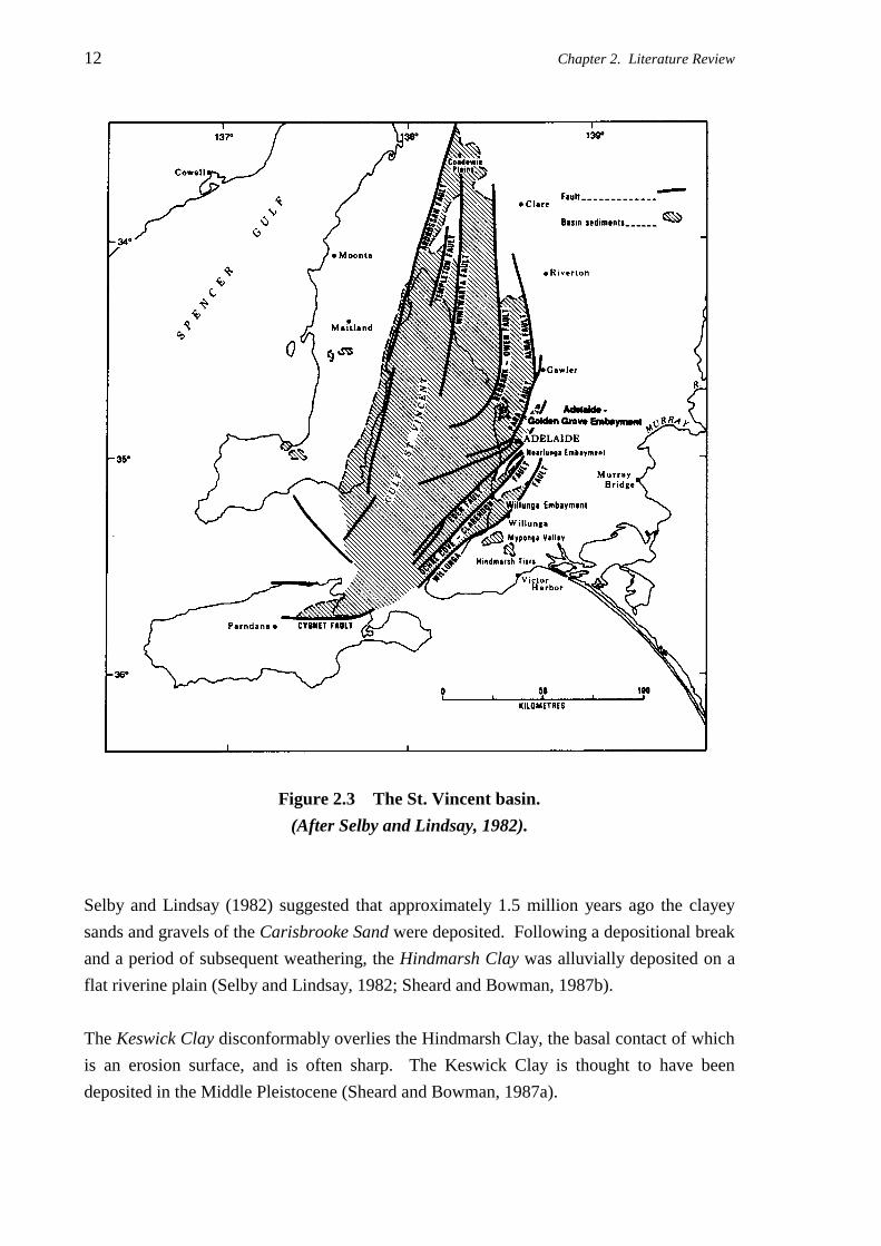
The St. Vincent Basin, shown in Figure 2.3, was formed by a downfaulted block bounded
by the Ardrossan Fault to the west and a series of major faults to the east. The Adelaide
city area is located in one of the eastern embayments of the St. Vincent Basin, referred to
by Selby and Lindsay (1982) as the Highbury - Golden Grove Embayment and later by
Sheard and Bowman (1987a) as the Adelaide - Golden Grove Embayment. The sediments

10 Chapter 2. Literature Review
Figure 2.2 The Adelaide city area.
(After Cox, 1970 and Selby and Lindsay, 1982).

Chapter 2. Literature Review 11
Table 2.1 Summary of stratigraphic units underlying the Adelaide city area.
(After Selby and Lindsay, 1982).
Era, Age in Geological MaximumPeriod, Millions Classification Thickness Material DescriptionEpoch of years Name (m)
Alluvium of Red brown Silty CLAY;
the River grades downwards to SAND
Cainozoic 10,000 Torrens and GRAVEL (SP-GP).
Quaternary years Callabonna Clay 21 Red brown CLAY (CH).
Holocene Pooraka Light brown Silty CLAY
Formation (CL-ML), calcareous with
layers of calcrete GRAVEL (GM).
Keswick 7 Grey-green CLAY (CH) with red and
Clay brown mottling, stiff to hard, fissured.
Cainozoic Hindmarsh 16 Grey-green CLAY (CH) with yellow and
Quaternary Clay red mottling with overlying SAND (SC).
Pleistocene 1.5 Carisbrooke 13 Yellow, orange brown and grey, fine to
Sand medium Clayey and Silty SAND (SC/SM)
Burnham 1 - 2 White Clayey, Sandy
Limestone and rubbly LIMESTONE.
Cainozoic Hallett Pale grey to brown
Tertiary 3 Cove 12 calcareous SANDSTONE
Pliocene Sandstone with layers of SAND (SP).
Port Sandy SILT and CLAY
30-38 Willunga 39 with strong CHERT nodules
Formation (GC-GP, ML, SM).
Chinaman Dark grey to black SILT and CLAY
Gully 12 (ML-CL) with layer of Gravelly,
Cainozoic Formation Clayey SAND (SC-GW).
Tertiary Blanche Alternating bands of cherty
Eocene Point 25 siltstone and grey SILT (SM)
Formation overlying green to dark grey Clayey
SAND (SC) and LIMESTONE.
South Maslin 12 Grey to brown or yellow, Silty
Sand SAND (SM) with pyrite lumps.
40 Clinton 27 Dark grey CLAY (CL) with lignite;
Formation irregular Clayey SAND zones (SC).
Proterozoic ≈ 800+ Adelaidean Brown, pink, grey to white, weathered
System SILTSTONE with quartz veinlets.
that filled these embayments were deposited first in swamps and from streams, followed by
several cycles of marine deposition. During the Tertiary period, movement along the faults
continued, as is evidenced by the variation of strata thickness adjacent to, and on either
side, of the faults.
12 Chapter 2. Literature Review
Figure 2.3 The St. Vincent basin.
(After Selby and Lindsay, 1982).
Selby and Lindsay (1982) suggested that approximately 1.5 million years ago the clayey
sands and gravels of the Carisbrooke Sand were deposited. Following a depositional break
and a period of subsequent weathering, the Hindmarsh Clay was alluvially deposited on a
flat riverine plain (Selby and Lindsay, 1982; Sheard and Bowman, 1987b).
The Keswick Clay disconformably overlies the Hindmarsh Clay, the basal contact of which
is an erosion surface, and is often sharp. The Keswick Clay is thought to have been
deposited in the Middle Pleistocene (Sheard and Bowman, 1987a).

Chapter 2. Literature Review 13
Following the deposition of the Keswick Clay, a major cold, dry and windy period began in
the Middle Pleistocene about 700,000 years ago. This led to the accumulation of a wind-
blown calcareous dust, or loess, known as the calcareous mantle. This is an extremely
variable soil profile which varies from nodular lime gravel to soft calcareous silt and clay.
Usually the calcareous material appears in white, yellow or pink patches within grey or
green sand, silt, or clay. In the Adelaide city area the calcareous mantle grades downwards
into the Keswick, or Hindmarsh, Clay, a transition which is marked by: the gradual
disappearance of carbonate nodules and patches; a change to stiff clay of high plasticity;
and development of mottling and structuring in the clay.
Approximately 20,000 years ago, following a period of faulting and erosion, alluvial silts
and clays of the Pooraka Formation were deposited. Another cold, dry period caused
further accumulation of windblown calcareous sediments which modified the Pooraka
Formation. Finally, a red-brown, non-calcareous, alluvial clay, known as the Callabonna
Clay, or Soil-B Horizon, was deposited over much of the Adelaide city area, where it is
usually less than one metre in thickness. In some parts of the Adelaide city area, the
Callabonna Clay is absent due to erosion, weathering, gilgai and shallow earthmoving
activities.
Subsequent to the deposition of the Keswick and Hindmarsh Clays, sediments were
deposited in the River Torrens valley. Though, at present, the River Torrens occupies a
relatively narrow channel within the Adelaide city area, below it lies a much wider ancient
valley. The sediments that have been deposited within this buried valley are known as the
Alluvium of the River Torrens, and deposition is thought to have occurred during the recent
Quaternary, since the Keswick and Hindmarsh Clays have been completely removed from
this valley (Selby and Lindsay, 1982). The composition of these sediments consists
generally of sandy gravel overlain by silt and clay, but vary greatly, both laterally and with
depth.
2.3.2 Geotechnical Characteristics
This section details the geotechnical characteristics of the Keswick and Hindmarsh Clays
relevant to this research. These characteristics include: stratigraphy; mineralogy; plasticity;
moisture regime; specific gravity; degree of saturation; instability index; and coefficient of
earth pressure at rest.

14 Chapter 2. Literature Review
2.3.2.1 Stratigraphy
Since the late 1800’s, many geoscientists have described the clay-rich deposits overlying
the Tertiary marine sediments of the Adelaide plains. These clays have been referred to as
Plio-Pleistocene ‘pipe clay’, Mammaliferous Drift, ‘alluvial mottled clays’, Adelaide Clay,
‘mottled clay’ and the Pleistocene Clay. Recently, Selby and Lindsay (1982) referred to
these clays as the Hindmarsh Clay and they described it as consisting of three layers: the
upper clay layer; the middle sand member; and the lower clay layer. Based on a joint
Department of Mines and Energy, S.A. and CSIRO project that incorporated the drilling of
62 boreholes in the Adelaide metropolitan area, Sheard and Bowman (1987a & b)
suggested that a disconformable erosion surface exists between the upper clay layer and the
lower sediments. They subsequently redefined the upper clay layer as the Keswick Clay
and the middle sand member and lower clay layer as the Hindmarsh Clay. However, it is
somewhat ambiguous to refer to this soil deposit, which consists of a layer of clay and a
layer of sand, as the “Hindmarsh Clay.” As a consequence, for the remainder of this thesis,
the term Hindmarsh Clay Formation will refer to both, the Hindmarsh Clay sand member
(the middle sand member of Selby and Lindsay, 1982), and the Hindmarsh Clay layer (the
lower clay layer of Selby and Lindsay, 1982), and the term Keswick Clay will be consistent
with that defined by Sheard and Bowman (1987a).
(i) Keswick Clay
The Keswick Clay underlies much of the Adelaide city area and pockets of the Adelaide
metropolitan area, as shown in Figure 2.4, and has been eroded by the River Torrens. It
stratigraphically overlies the Hindmarsh Clay Formation; the basal contact surface being a
disconformable erosion surface.
Keswick Clay is a relatively uniform, very stiff to hard, silty clay of high plasticity. It has a
Unified Soil Classification System (USCS) symbol of CH and is heavily fissured, with
fissure spacings of approximately 10 to 25 mm. Its colour varies from grey-green to
yellow-grey (gley colours) with red (haematite) and yellow (limonite) mottling of varying
proportions. Sheard and Bowman (1994) suggest that the gley colours may have resulted
from post-depositional chemical reduction in oxygen-poor groundwaters. Within the
Adelaide city area, its thickness varies to a maximum of approximately 7 metres. Tree
roots have been found at all depths and are probably the remains of old eucalypts removed
during urbanisation (Cox, 1970).

Chapter 2. Literature Review 15
Figure 2.4 Distribution of the Keswick Clay.
(After Sheard and Bowman, 1987a).
Stapledon (1970) and Selby and Lindsay (1982) suggested that the Keswick Clay has been
overconsolidated due mainly to desiccation, with preconsolidation pressures in excess of
400 kPa.
(ii) Hindmarsh Clay Sand Member
The Hindmarsh Clay sand member consists of a grey and brown, dense, coarse clayey sand
(USCS symbol SC). It directly overlies either the clay member of the Hindmarsh Clay
Formation, the Hallett Cove Sandstone, or the Blanche Point Formation (Cox, 1970). The
16 Chapter 2. Literature Review
sand has many red lateritic and sand/rock pebbles, some horizontal interbedded clay layers
and traces of calcareous material.
Selby and Lindsay (1982) suggested that the sand member is distributed in an elongated
zone extending south-southwest across the central city area and that the member probably
represents a river channel deposit.
(iii) Hindmarsh Clay Layer
The Hindmarsh Clay Layer underlies the Adelaide city area and much of the Adelaide
metropolitan area, as shown in Figure 2.5. In the Adelaide - Golden Grove Embayment the
River Torrens has dissected the unit.
The Hindmarsh Clay layer is similar in appearance and properties to that of the Keswick
Clay. It is a very stiff to hard, highly plastic silty clay (USCS symbol CH). Selby and
Lindsay (1982) attribute stiffening of the upper 1 to 2 metres of the clay, which they term
‘pseudo-consolidation’, to post-depositional desiccation. Its colour is the same as the
Keswick Clay, that is, grey-green with red and yellow mottling at depth. The Hindmarsh
Clay Layer directly overlies the Carisbrooke Sand or, where it has been removed by
erosion, it overlies the Hallett Cove Sandstone. (The Burnham Limestone is often seen
only as a transitional zone within the Hallett Cove Sandstone). The Hindmarsh Clay Layer
is relatively uniform, both in properties and in surface level.
Where no sand separator bed exists, and where the Hindmarsh and Keswick Clays are
similar in character, the boundary between the two units is difficult to establish (Sheard and
Bowman, 1987b). Like the Keswick Clay, the Hindmarsh Clay layer is heavily fissured
with large and numerous slickensides which occur at 30° to 45° to the horizontal.
Structural features associated with these clays are treated in greater detail in §2.3.3.
2.3.2.2 Mineralogy
In general, very few tests have been carried out in order to determine the mineralogy of the
Keswick and Hindmarsh Clays. This holds true not only for these clays, but for all
Adelaide soils in general. Cox (1970) cited X-ray diffraction tests carried out on the
Keswick Clay which indicated that the soil consists predominantly of three clay minerals:
illite; kaolinite; and montmorillonoid minerals. Illite appears in quantities generally greater
than 50%, whereas kaolinite was found in quantities in excess of 20%. Minerals of the
montmorillonoid group were observed in amounts of less than 20%.

Chapter 2. Literature Review 17
Figure 2.5 Distribution of the Hindmarsh Clay.
(After Sheard and Bowman, 1987b).
Stapledon (1970) suggested that the Hindmarsh Clay consists of illite and kaolinite in
proportions of greater than 50%, and lesser amounts of montmorillonite. It is not evident
whether Stapledon was referring to the Keswick Clay or the Hindmarsh Clay layer,
however, Stapledon (1995) confirmed that he was referring to both.

18 Chapter 2. Literature Review
2.3.2.3 Plasticity
Cox (1970) presented the results of many Atterberg limit tests performed on samples of
Keswick Clay and the Hindmarsh Clay layer in the Adelaide city area. The ranges of
results from these tests are summarised in Table 2.2.
Table 2.2 Summary of Atterberg limit tests. (Reported by Cox, 1970).
Member No. oftests
wP
(%)wL
(%)IP
(%)Clay
Content (%)Activity
Keswick Clay 75 18-29 60-117 42-88 52-67 0.8-1.2
Hindmarsh Clay layer 11 16-30 55-100 40-70 50-70 0.7-1.0
Cox suggested that the plastic limit, liquid limit, plasticity index and activity increase to the
north. Sheard and Bowman (1994) also reported Atterberg limit results based on their
extensive study of soils in the metropolitan area of Adelaide. Those results that pertain to
soils within the Adelaide city area are summarised in Table 2.3, with average values shown
in parentheses. Undifferentiated Keswick-Hindmarsh Clay refers to soil that the authors
were unable to classify as Keswick Clay or the Hindmarsh Clay layer.
Table 2.3 Summary of Atterberg limit tests.
(Reported by Sheard and Bowman, 1994).
Member No. oftests
wP
(%)wL
(%)IP
(%)Keswick
Clay17 21-35
(27)46-98(74.6)
25-63(47.6)
Hindmarsh Claylayer
14 17-42(26.9)
46-100(72.4)
27-66(45.5)
UndifferentiatedKeswick-Hindmarsh Clay
9 12-32(23.8)
77-96(83.7)
53-84(59.9)
Note: Average values are shown in parentheses.
2.3.2.4 Moisture Regime
Cox (1970) suggested that the in situ moisture content of the Keswick Clay generally
decreases from 34% at the surface of the layer to 30% at depth, with moisture contents of

Chapter 2. Literature Review 19
up to 40% beneath old basement floors. He also reported that the in situ moisture content
of the Hindmarsh Clay is much lower than that of the Keswick Clay, varying from 20% at
the surface of the clay layer to 30% at depth.
Jaksa and Kaggwa (1992) presented a moisture distribution of far greater variation than
that suggested by Cox. Based on the results of 451 separate tests performed on samples of
Keswick Clay obtained throughout the Adelaide city area, Jaksa and Kaggwa suggested
that the in situ moisture content varied anywhere between 15% and 40% at depths between
one and 20 metres below ground surface. These data are examined in greater detail in
Chapter 6.
2.3.2.5 Specific Gravity
Based on the results of three laboratory tests performed on samples of Keswick Clay, Cox
(1970) reported that the average specific gravity of solids, Gs , was 2.70. The values of the
individual tests, however, were not published. Jaksa and Kaggwa (1992) suggested that a
mean value of 2.75 ± 0.02 would be a more appropriate value for the Gs of the Keswick
Clay. Their estimate was not based on laboratory test measurements of Gs , but on a
statistical analysis of 451 moisture content and dry density test results, as well as an
estimation based on the mineralogy of the clay particles. Islam (1994) reported the result
of a single laboratory test which was carried out on a sample of Keswick Clay obtained
from the Myer-Remm development, which lies within the Adelaide city area. He reported
the Gs of the clay to be 2.73. To date, no values of the Gs of the Hindmarsh Clay have been
published.
2.3.2.6 Degree of Saturation
In general, the in situ degree of saturation, Sr , is obtained from the measured in situ
moisture content, w, and dry density, ρd; tabulated values of the density of water, ρw
(usually assumed constant at 1000 kg/m3); and the value of the specific gravity of solids,
Gs , via the relationship shown in Equation (2.1), below.
( ) dws
dsr G
GwS
ρ−ρρ=
(2.1)
Using this relationship, and a Gs of 2.70, Cox (1970) found that the majority of his samples
of Keswick Clay, taken from 20 separate sites within the Adelaide city area, had degrees of
saturation between 95% and 100%. He inferred that the Keswick Clay was fully saturated

20 Chapter 2. Literature Review
by suggesting the 0% to 5% air which was measured could be attributed to air entering the
fissure system during sampling and testing. Cox claimed, based on theoretical calculations,
“ that fissures with a spacing of one inch [25 mm] need open only 0.0001 in. [0.0025 mm]
to give a degree of saturation of 95%.” Similar calculations performed by the author
suggest that the fissures need to open 0.02 mm to yield an Sr of 95%. In addition,
Stapledon (1970) stated that the Hindmarsh Clay (the Keswick Clay and Hindmarsh Clay
Formation) is either unsaturated or quasi-saturated, that is, apparently saturated, but
showing appreciable negative porewater pressures.
Using 451 test results, Jaksa and Kaggwa (1992) also concluded that the majority of the
Keswick Clay is “saturated or very close to being saturated.” They also described the clay
as being quasi-saturated due to the fact that, though it is saturated, no free moisture is
observed. These data will be examined in greater detail in Chapter 6.
2.3.2.7 Instability Index, Ipt
The instability index, Ipt, is defined as the ratio between the vertical strain, εv, and the
change in total suction, ∆u, as shown in Equation (2.2).
Iuptv= ε
∆(2.2)
The Ipt is a measure of the reactivity or expansiveness of a soil, or in other words, the
amount of shrinkage or swelling that the soil will undergo upon drying or wetting,
respectively. It is widely accepted that the Keswick and Hindmarsh Clays are extremely
expansive with recorded measurements of Ipt up to 6% not uncommon (Sheard and
Bowman, 1994). One would suspect that the reactivity of these clays is related to the
amount of montmorillonoid minerals present in the soil mass, however, no published
mineralogical tests have yet been carried out to investigate this assumption.
2.3.2.8 Coefficient of Earth Pressure at Rest, K0
The coefficient of earth pressure at rest, K0, is defined as the ratio between the horizontal
effective stress, σ'h, and the vertical effective stress, σ'v, at some depth below the ground
surface, as shown in Equation (2.3).
K h
v0 =
σσ
’
’(2.3)

Chapter 2. Literature Review 21
Richards and Kurzeme (1973) installed earth pressure cells and psychrometer probes
behind a 7.5 metre deep basement wall, much of which was retaining undifferentiated
Keswick-Hindmarsh Clay. They found that after a period of approximately two years, the
earth pressures stabilised to a value of 1.3 to 4 times the overburden pressure. Similar
results have been obtained from self-boring pressuremeter tests performed in the Keswick
and Hindmarsh Clays (Kaggwa, 1992).
While Richards and Kurzeme’s measurements were based on total stresses, many
geotechnical engineering practitioners used these results to imply that the Keswick and
Hindmarsh Clays have values of K0 up to 4. This high value of K0 has been used by some
engineers to hypothesise that the lateral earth pressure is close to the passive resistance of
the soil (Kaggwa, 1992).
Kaggwa (1992) examined self-boring pressuremeter, triaxial and psychrometer test results
obtained from an extensive site investigation for a proposed tunnel within the Adelaide city
area (Coffey and Partners Pty. Ltd., 1979). He found, by assuming that measurements of
soil suction could be equated to negative porewater pressures, that the derived values of K0
reduced to more realistic figures in agreement with laboratory K0 triaxial tests. Kaggwa
suggested that values close to 1 are appropriate for the K0 of the Keswick and Hindmarsh
Clays.
2.3.3 Structural Features
Stapledon (1970) detailed many structural features and defects within the Keswick Clay
and the Hindmarsh Clay Formation. These included:
• Steeply dipping joints: These dip between 60° and vertical, are generally less than
4 m2 in areal extent and, upon drying, cause the clays to
break into prismatic or polyhedral blocks 20 to 200 mm in
width. The faces are slickensided, which suggests that they
may have been initially formed by tension due to drying
out, and then modified by shearing due to movement of
adjacent blocks.
• Gently dipping joints: Slickensided joints with dips ranging from 20° to 60° and
extending for several metres. These joints generally occur
in two sets striking approximately parallel to one another,
but dipping in opposite directions.
22 Chapter 2. Literature Review
• Fissures: These are joints of small areal extent, generally less than
0.2 metres, which may have originated during deposition
of the clay in large open-structure flocs.
• Dykes: These are found only in the Keswick Clay and are
numerous where the clay has come in contact with sandy
topsoil. They are generally 1 to 5 mm wide and are
thought to have formed by the percolation of the sandy
topsoil into the vertical joints.
• Other minor defects: These include roots, ranging up to 10 mm in diameter;
tubes; tube-casts; and tunnels and sinkholes.
In addition, Stapledon (1970) stated that some of these joints may have apertures as wide as
5 mm. Further, he suggested that all of these macroscopic and structural defects greatly
influence the engineering behaviour and the vertical permeability of the clay masses,
though the extent of this influence is extremely difficult to assess quantitatively.
2.3.3.1 Gilgais
The term gilgai refers to dome-type undulations of the upper surface of the Keswick Clay
and Hindmarsh Clay Formation as shown in Figure 2.6. An abundance of gilgai in the
Adelaide city area gives rise to marked lateral variation in soil type for the first few metres
below the ground surface.
Stapledon (1970) proposed a scenario for the development of gilgai structures, a summary
of which is given below, and a graphical representation is shown in Figure 2.7.
1. Firstly, the Keswick and Hindmarsh Clays were deposited in a flocculated state in a
river flood plain.
2. Subsequently, the surface of the clay dried, cracked and became desiccated, largely as a
result of uplift. This resulted in the formation of numerous vertical shrinkage cracks
and the pseudo-consolidation of the clays, referred to earlier.
3. Wind-blown quartz sand and calcareous silt accumulated on the surface of the clay and
penetrated and filled the cracks and open joints to form dykes.
4. Subsequent wetting, which led to the deposition of the red-brown Callabonna Clay,
resulted in the swelling of the Keswick and Hindmarsh Clays.

Chapter 2. Literature Review 23
Figure 2.6 Typical gilgai structures within the Adelaide city area.
(After Selby and Lindsay, 1982).
5. The pressures induced by the increased moisture resulted in upward swelling and
doming of the clays, as it was largely unconfined in the vertical direction. Horizontally,
the clay was confined by the surrounding soil mass and lateral swelling resulted in the
formation of the gently dipping joints as a consequence of shear failure.
The gilgai structures appear to be relatively recent in origin as they have displaced soil-
profile horizons (Selby and Lindsay, 1982). It appears that most of the gilgais are inactive,
though it is thought that they could be reactivated by a local increase in groundwater flow.

24 Chapter 2. Literature Review
Figure 2.7 Suggested origin of gilgai structures.
(After Stapledon, 1970 and Selby and Lindsay, 1982).
2.3.4 Groundwater
The general groundwater table is usually encountered in the Hallett Cove Sandstone and,
in addition, perched groundwater tables often occur within the upper three metres of the
Keswick Clay (Cox, 1970 referred to this as the upper perched water table) and within the
sand member of Hindmarsh Clay Formation (the lower perched water table). The extent of
the upper perched water table varies irregularly over any one site, due mainly to level
variations of the boundary between the calcareous mantle and the Keswick Clay, as a result
of gilgai. Movement of this groundwater is facilitated by the joints within the clay mass.
Cox (1970) suggested that groundwater within the Adelaide city area originates from the
foothills to the east, and Selby and Lindsay (1982) indicated that the Hallett Cove
Sandstone has been extensively used as a drainage horizon to take seepage water which
collects beneath buildings in the city area.
Chapter 2. Literature Review 25
2.3.5 Summary
This section has examined the geotechnical and structural characteristics of the Keswick
and Hindmarsh Clays, as well as the general groundwater regime within the Adelaide city
area. It has been shown that these clays are: relatively homogeneous; significantly fissured
- both in the macro and micro scales; highly plastic; extremely expansive; and exhibit
geotechnical properties similar to those of the well-documented London Clay.
The Keswick and Hindmarsh Clays will form the basis of an experimental investigation to
quantify the spatial variability of these soils. This investigation will measure strength
parameters of these clays by means of the cone penetration test, which is detailed below.
2.4 THE CONE PENETRATION TEST
This section discusses aspects of the cone penetration test which relate directly to the study
of spatial variability. These include: equipment; test procedure; applications and data
interpretation; determination of the undrained shear strength; extent of the failure zone; and
accuracy of the test itself. As discussed in Chapter 1, the cone penetration test was used in
this study to evaluate the small-scale spatial variability of the Keswick and Hindmarsh
Clays.
2.4.1 Introduction
The electrical cone penetration test (as distinct from the mechanical cone penetration test,
and commonly referred to by the shorter name of cone penetration test, CPT) essentially
involves pushing a steel cone and rods, of standard dimensions, into the subsurface profile
and monitoring the resistance to penetration mobilised in the soil.
Since it was first developed in Holland in 1965, the CPT has continued to gain wide
acceptance in many countries throughout the world. De Ruiter (1981) attributed its
increased worldwide use to three main factors:
1. The electric cone penetrometer provides more precise measurements, and improvements
in the equipment allow deeper penetrations, particularly in dense materials.
26 Chapter 2. Literature Review
2. The need for penetration testing as an in situ technique in offshore foundation
investigations, in view of the difficulties in achieving adequate sample quality in marine
environments.
3. The addition of other simultaneous measurements to the standard friction penetrometer,
such as porewater pressure and soil temperature.
De Ruiter (1981) stated that the CPT is the only available routine technique that provides
an accurate continuous profile of soil stratification.
2.4.2 Equipment
The electric cone penetrometer consists, essentially, of two strain gauge load cells; one
being attached to the cone tip and measuring cone tip resistance, qc; and the other,
connected to the side, or sleeve, of the cone penetrometer and measuring sleeve friction, fs .
The cone tip resistance, qc , is defined as the total force acting on the cone tip, Fc , divided
by the area of the base of the cone, Ab , and is usually expressed in units of MPa. The
sleeve friction, fs , is defined as the total force on the friction sleeve, Fs , divided by the
surface area of the sleeve, As , and is usually expressed in units of kPa. A schematic
representation of the electric cone penetrometer is shown in Figure 2.8.
The load cells contain a number of electrical resistance strain gauges which are arranged in
such a manner that automatic compensation is made for bending stresses and only axial
stress is measured (de Ruiter, 1971). The push rods, used to advance the electric cone
penetrometer into the subsurface profile, are usually of a standard length of one metre with
a tapered thread, male at the lower end and female at the upper. In addition, the rods have
a hollow core so that the cone penetrometer cable can pass through each rod enabling the
electronics of the cone to be connected to the recording instruments located at the ground
surface.
As will be discussed in greater detail in §3.2, the recording devices generally consist of two
types: analogue and digital. These instruments measure qc and fs , and in some cases, depth
of the cone penetrometer.
The equipment and procedure of the CPT vary throughout the world. Over the years, many
committees have been formed in an attempt to establish a consistent, worldwide standard
for the CPT; the most recent of these being at the First International Symposium on
Penetration Testing (ISOPT-1) (De Beer et al., 1988). In addition, some countries have
established individual standards for the CPT, the most relevant of these, for this research,

Chapter 2. Literature Review 27
Figure 2.8 Schematic diagram of the electric cone penetrometer.
(After Holtz and Kovacs, 1981).
being the American Standard, ASTM D3441 (American Society for Testing and Materials,
1986), and the Australian Standard, AS 1289.F5.1 (Standards Association of Australia,
1977). In general, these three standards agree on the fundamental aspects of the CPT
equipment and procedure. Relevant details of the CPT equipment, as specified in these
standards, are summarised briefly below and the standard procedure is detailed in §2.4.3.
• The standard cone has a base diameter of 35.7 mm and an apex angle of 60° resulting in
a projected area of 1000 mm2 (10 cm2). The gap between the cone and other elements of
the penetrometer shall not be greater than 5 mm.

28 Chapter 2. Literature Review
• The diameter of the standard friction sleeve is 35.7 mm and has a surface area of
15,000 mm2 (150 cm2). The friction sleeve is located immediately above the cone.
• Both the cone and sleeve shall be made from steel of a type and hardness suitable to
resist wear due to abrasion by soil. The cone shall have, and maintain with use, a
roughness of ≤ 1 µm, and the friction sleeve shall have a roughness of 0.5 µm ± 50%.
• No standard details for the electrical measuring equipment are given.
• The thrust machine shall have a stroke of at least one metre and shall push the rods into
the soil at a constant rate of penetration. The thrust machine shall be anchored and/or
ballasted such that it does not move relative to the soil surface during the pushing
action.
• Where a friction reducer2 is used, it shall be located at least one metre above the base of
the cone.
2.4.3 Procedure
The standard CPT procedure detailed in ISOPT-1 (De Beer et al., 1988), ASTM D3441
(American Society for Testing and Materials, 1986), and AS 1289.F5.1 (Standards
Association of Australia, 1977) is summarised as follows:
1. The thrust machine, generally some form of drilling rig, is set up over the test location
and is oriented as near to vertical as practicable. The deviation from vertical shall not
exceed 2%.
2. The penetrometer and the first length of rod assembly are connected to the thrust
machine, the penetrometer being passed through the rod guide at the base of the
machine. Prior to connection, the push rods have been pre-threaded with the electrical
cable.
3. The cone penetrometer is thrust a short distance into the soil and allowed to remain
there until the temperature of the tip has equilibrated with the temperature of the ground,
usually between 5 and 10 minutes.
4. The penetrometer is withdrawn from the soil and the cone tip and sleeve friction
transducers are zeroed, whilst protecting the cone from direct sunlight.
2 narrow local protuberances outside the push rod surface, placed above the penetrometer tip, and provided to reduce the
total friction on the push rods.
Chapter 2. Literature Review 29
5. The cone penetrometer is advanced into the subsurface profile at a constant rate of
20 mm/s (±5 mm/s). Whilst this is occurring, depth, qc and fs are recorded. Under no
circumstances shall the interval between the readings be greater than 0.2 metres. The
depths shall be measured to an accuracy of at least 0.1 metres.
6. Once the thrust mechanism has reached the end of its travel, the rod assembly is
disconnected from it, the thrust machine is raised and additional push rods are attached
as required.
7. Steps 5 and 6 are continued until the required test depth is reached.
8. On completion of the test, the rod assembly and cone penetrometer are removed from
the soil. A final set of readings is taken and compared with the initial readings. If these
are not satisfactory, the results are discarded and the penetrometer is either repaired or
replaced and the test is repeated.
2.4.4 Applications and Data Interpretation
The CPT is ideally suited for use in fine-grained soils and in sands, both on land and
offshore. Due to the probability of cone damage and thrust limitations, the CPT is rarely
used in gravels, and weak and weathered rock profiles.
Orchant et al. (1988) suggested that the information obtained from the CPT can be used to
interpret the following geotechnical characteristics: soil classification; relative density, RD,
of sands; friction angle, φ, of sands; undrained shear strength, su , of cohesive soils;
overconsolidation ratio, OCR; Young’s modulus of elasticity, E; compressibility of clay;
pile bearing capacity; shallow foundation bearing capacity; and liquefaction potential of
sands. The friction ratio, FR, is often used in conjunction with qc to assist in soil
classification. The friction ratio is defined as the ratio between fs and qc, and is usually
expressed as a percentage, as shown in Equation (2.4).
Ff
qRs
c
= × 100% (2.4)
Schmertmann (1978) and AS 1289.F5.1 (Standards Association of Australia, 1977)
emphasised that incorrect calculations of FR will be made unless a depth correction, or
shift, is applied to the fs measurements. This correction is required since the cone tip
resistance and sleeve friction load cells are physically separated by a given distance, and
hence measurements of qc do not refer to the same soil as that at which measurements of fs
are taken. Schmertmann (1978) recommended that this shift distance be the distance
30 Chapter 2. Literature Review
between the base of the cone and the mid-height of the sleeve which, in standard electric
cone penetrometers, is approximately 75 mm. Campanella et al. (1983) suggested that the
shift distance, also termed the friction-bearing offset, is 100 mm and is dependent on the
type of soil being penetrated. The shift distance is examined in detail in §5.3.5.
As mentioned above, CPT data are often used to determine the axial bearing capacity of
piled foundations. In fact, the CPT was essentially developed to facilitate the design of
driven piles (Orchant et al., 1988). As a consequence, a large number of pile design
methods have been developed which are based directly on CPT data. Robertson et al.
(1988) compared the results of 6 full-scale pile load tests with the predictions given by 13
separate static axial pile capacity prediction methods, each of which are based on CPT data.
Robertson et al. (1988) concluded that, in order of highest to lowest accuracy, the LCPC
Method (Bustamante and Gianeselli, 1982), the de Ruiter and Beringen Method (de Ruiter
and Beringen, 1979), and the Schmertmann and Nottingham Method (Schmertmann, 1978)
yielded the best predictions. Briaud (1988) also compared the predictions of 6 CPT axial
pile capacity methods using the results of 98 pile load tests. The 6 CPT pile methods that
Briaud examined included: the LCPC Method; the de Ruiter and Beringen Method; and the
Schmertmann and Nottingham Method. Briaud (1988) found that, overall, the LCPC
Method yielded the best predictions. As a consequence of its performance, the LCPC
Method, of Bustamante and Gianeselli (1982), will be used in Chapter 8 to assess the
significance of spatial variability on the design of pile foundations. The technique, itself,
will be described in detail in §8.3.1.
2.4.5 Determination of the Undrained Shear Strength of a Clay fromthe CPT
The CPT, and the majority of in situ tests, induce relatively rapid local failures in the soil
mass that allow little drainage in the clays. As a result, the cone tip resistance, qc, is
generally related to the undrained shear strength, su, by Equation (2.5), which is based on
the bearing capacity of a deep, circular foundation (Ladd et al., 1977; Schmertmann, 1978;
de Ruiter, 1982; Jamiolkowski et al., 1982; Sutcliffe and Waterton, 1983).
sq
Nuc v
k
=− σ 0 (2.5)
where: qc is the cone tip resistance;
σv0 is the total in situ vertical overburden stress;
Nk is the cone factor.
Chapter 2. Literature Review 31
The cone factor, Nk , is an empirically derived parameter usually obtained by cone
penetration testing in parallel with reference determinations of su . The undrained shear
strength, su , is normally obtained from triaxial tests performed on high quality specimens,
or from in situ vane shear tests - triaxial testing providing better estimates of Nk in most
situations (Sutcliffe and Waterton, 1983; Kay and Mayne, 1990). Sutcliffe and Waterton
(1983) suggested that the sleeve friction, fs , of the clay be used as a lower bound for su .
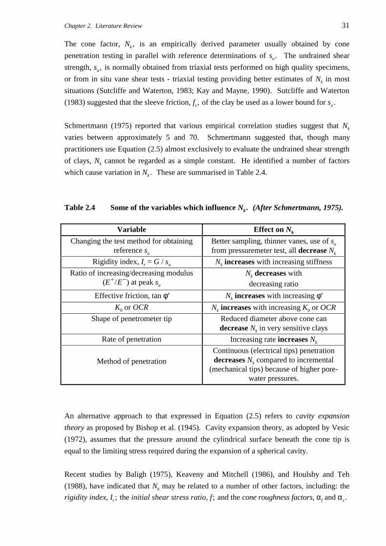
Schmertmann (1975) reported that various empirical correlation studies suggest that Nk
varies between approximately 5 and 70. Schmertmann suggested that, though many
practitioners use Equation (2.5) almost exclusively to evaluate the undrained shear strength
of clays, Nk cannot be regarded as a simple constant. He identified a number of factors
which cause variation in Nk . These are summarised in Table 2.4.
Table 2.4 Some of the variables which influence Nk. (After Schmertmann, 1975).
Variable Effect on Nk
Changing the test method for obtainingreference su
Better sampling, thinner vanes, use of su
from pressuremeter test, all decrease Nk
Rigidity index, Ir = G / su Nk increases with increasing stiffness
Ratio of increasing/decreasing modulus(E+/E−) at peak su
Nk decreases withdecreasing ratio
Effective friction, tan φ’ Nk increases with increasing φ’
K0 or OCR Nk increases with increasing K0 or OCR
Shape of penetrometer tip Reduced diameter above cone candecrease Nk in very sensitive clays
Rate of penetration Increasing rate increases Nk
Method of penetrationContinuous (electrical tips) penetrationdecreases Nk compared to incremental
(mechanical tips) because of higher pore-water pressures.
An alternative approach to that expressed in Equation (2.5) refers to cavity expansion
theory as proposed by Bishop et al. (1945). Cavity expansion theory, as adopted by Vesic
(1972), assumes that the pressure around the cylindrical surface beneath the cone tip is
equal to the limiting stress required during the expansion of a spherical cavity.
Recent studies by Baligh (1975), Keaveny and Mitchell (1986), and Houlsby and Teh
(1988), have indicated that Nk may be related to a number of other factors, including: the
rigidity index, Ir ; the initial shear stress ratio, f; and the cone roughness factors, αf and αs .

32 Chapter 2. Literature Review
Baligh (1975), and Houlsby and Teh (1988), suggested that Equation (2.5) should strictly
be written in terms of the in situ horizontal stress, σh0, instead of the vertical stress, σv0.
As a result, Equation (2.5) can be rearranged in the following manner:
0
000
0
000
0000
2
1
2 :where
2=
22=
vuu
hv
u
hck
u
hv
u
hc
u
h
u
h
u
vc
u
vck
s
K
sf
fs
qN
ss
q
sss
q
s
qN
σ−=σ−σ=
−σ−
σ−σ−σ−
σ−σ−σ−=σ−=
(2.6)
The parameter, f, is defined as the initial shear stress ratio and was originally proposed by
Davis and Poulos (1968) and more recently by Ladd et al. (1977). Theoretically, f can vary
between −1 (which represents passive failure in swelling soils under total stress
conditions) and +1 (which represents conditions at the maximum depth of a shrinkage
crack in terms of total stresses) (Kay and Mayne, 1990).
As suggested by Kay and Mayne (1990), it is convenient to use f to compare the various
proposals for the determination of Nk . Baligh (1975) proposed that Nk be calculated based
on a strain path approach, as follows:
( )N I fk r= + −12 2ln (2.7)
Keaveny and Mitchell (1986) used spherical cavity expansion theory and suggested that Nk
be determined using the mean stress, p, instead of σv0. Kay and Mayne (1990) rewrote
Keaveny and Mitchell’s equation as:
( )( )fIN rk −+= ln33.142.3 (2.8)
Baligh (1986) pointed out that an inconsistency in the application of the cavity expansion
theory to cone penetration problems is that it does not correctly model the strain paths
followed by soil elements. Teh and Houlsby (1991) presented the results of a strain path
approach to the steady penetration of a cone in homogeneous soil. This involved changing
the frame of reference and treating the penetration process as a steady flow of soil past a
stationary penetrometer. As an initial estimate of the flow field, the soil was treated as a
viscous fluid. The authors found that the cone factor, Nk, was significantly influenced by
the rigidity index, Ir , of the soil and the in situ stress conditions, f, and, to a lesser extent,

Chapter 2. Literature Review 33
by the roughness of the cone and shaft, αf and αs3. In addition, Teh and Houlsby (1991)
concluded that the in situ horizontal stresses have a greater influence on Nk than the vertical
stress. Using a strain path approach, and assuming initial isotropic soil stresses and a
simple, linear, elastic, perfectly-plastic model with a von Mises yield surface, Teh and
Houlsby (1991) concluded that Nk can be determined using:
( )N I fk r f= + + −1.25 1.84 ln 2 2α (2.9)
However, since the stresses derived using the strain path method do not fully satisfy the
equilibrium condition, because of errors in the assumed initial displacement field, Teh and
Houlsby (1991) carried out a strain path finite element analysis. The authors found that Nk
can be determined using Equation (2.10).
( )[ ] fI
IN sfr
rk 8.12.02.42000
1.25ln13
4 −α−α+
++= (2.10)
where: 50 ≤ Ir ≤ 500
The authors stated that, although Equation (2.10) results in higher cone factors than have
previously been derived theoretically, the cone factors are closer to those observed in
practice and therefore provide a more reasonable solution to the cone penetration problem.
Kay and Mayne (1990) applied Equations (2.5) and (2.10) to CPT and screw plate load test
data obtained from a number of site investigations performed in Adelaide (Mitchell and
Kay, 1985). Using f = −0.4 and αf = αs = 0.8, values judged to be appropriate for the
highly overconsolidated fissured plastic clays and the very stiff silty and sandy clays that
constituted the soils tested, Kay and Mayne (1990) found that values of Nk obtained from
Equation (2.10) yielded good predictions of undrained shear strength, su , when compared
to measured values.
The relative importance of the expressions given in Equations (2.5) and (2.7) to (2.10) will
be discussed in detail in Chapter 4.
3 both αf and αs lie within the range 0 and 1, where ατ
ff
us=
3
2; α
τs
s
us=
3
2; and τf and τs are the shear stresses on
the cone and sleeve respectively.

34 Chapter 2. Literature Review
2.4.6 Extent of the Failure Zone Due to Cone Penetration
As it is advanced into the subsurface profile, the cone penetrometer causes a zone of soil to
fail and deform plastically. Teh and Houlsby (1991), using a strain path approach as
discussed in the previous section, quantified the extent of this failure zone by the use of
two parameters: rp - the radial distance of the plastic boundary from the axis of penetration
measured at a large enough distance above the cone tip; and zp - the distance between the
cone tip and the plastic boundary measured along the axis of the penetrometer. The
parameters rp and zp , as well as the two possible states of the elasto-plastic boundary as
defined by Teh and Houlsby (1991), are shown diagrammatically in Figure 2.9.
βo
Plastic Soil
Plastic Soil
Elastic Soil
Elastic Soil
zp
rp
ac
Figure 2.9 Schematic representation of rp and zp .
(Adapted from Teh and Houlsby, 1991).
Figure 2.10 illustrates the variation of the parameters rp and zp with the rigidity index, Ir .
Teh and Houlsby (1991) found close agreement with cylindrical and spherical cavity
expansion solutions, as shown in Figure 2.10. For a standard cone with β = 60°,
ac = 35 7 2. = 17.9 mm, and a rigidity index typical for the Keswick and Hindmarsh Clays,
that is, Ir = 100, Figure 2.10 suggests that rp ≈ 150 mm and zp ≈ 90 mm. These values
compare well to those obtained by Baligh (1986), who, using a spherical cavity expansion
model and a Prandtl-Reuss bilinear clay, found that rp ≈ 180 mm and zp ≈ 110 mm.
These dimensions imply that the measurements of qc and fs , obtained by the CPT, are not

Chapter 2. Literature Review 35
Figure 2.10 Location of the elasto-plastic boundary in cone penetration.
(After Teh and Houlsby, 1991).
point values, but rather block values; that is, measurements based on the failure of a
volume of soil surrounding both the cone and sleeve. The implications of this will be
treated in Chapter 5.
2.4.7 Accuracy of the CPT
Errors associated with measurement can be separated into two categories: systematic errors
and random errors (Lee, White and Ingles, 1983; Baecher, 1986; Orchant et al., 1988; Kay,
1990).
Systematic errors, or bias, are the consistent underestimation or overestimation of a
measured parameter. Orchant et al. (1988) separated systematic errors into: equipment
errors - inaccuracies associated with such effects as drift, non-linearities, zero error of the
elements of the measuring instrument; and operator/procedural errors - variabilities
associated with limitations in existing test standards and between different operators.
Random errors, or scatter, are the variation of test results which cannot be directly
attributed to the inherent variability of the material (spatial variability), equipment errors or
operator/procedural errors. Random errors are quantified by performing many tests under

36 Chapter 2. Literature Review
identical conditions, and are assumed to have a mean of zero, thus affecting test results
equally, and without bias.
Orchant et al. (1988) suggested that the total measurement error can be evaluated by the
following model:
σ σ σ σ
σ
σ
σ
σ
measure equip op proc random
measure
equip
op proc
random
2 2 2 2
2
2
2
2
= + +
=
=
=
=
/
/
where: total variance of measurement;
variance of equipment effects;
variance of operator / procedural effects;
variance of random testing effects.
(2.11)
Equation (2.11) has two important assumptions: (i) all of the sources of uncertainty can be
considered as additive; and (ii) each source of measurement error is considered to be
independent, or uncorrelated. In order to simplify the model, Orchant et al. (1988) adopted
the second assumption. Otherwise if the sources of error are correlated, covariance terms,
expressing the inter-relationship between the parameters, would need to be included and
evaluated, thereby complicating the model considerably.
Each of these sources of measurement error are discussed in the following sections.
2.4.7.1 Equipment Errors of the CPT
Orchant et al. (1988) attributed CPT equipment errors to a number of variables. These are
summarised in Table 2.5.
Table 2.5 Variables contributing to CPT equipment error.
(After Orchant et al., 1988).
Variable Relative Effect on CPT ResultsCone Size Minor
Cone Angle Moderate to SignificantManufacturing Defects Minor to Moderate
Leaky Seals MinorExcessive Cone Wear Minor to Moderate

Chapter 2. Literature Review 37
Durgunoglu and Mitchell (1975) found that the angle of the cone tip has an important
effect on CPT results, and that an angle of 60° favours maximum penetration for a given
force on the penetrometer. Baligh et al. (1979) also supported this conclusion, having
tested cones with angles of 18°, 30° and 60°. The authors found that by using an 18° cone,
measurements of qc and fs were increased by as much as 30% of those obtained by using the
standard 60° cone.
De Ruiter (1981) detailed the use of enlarged cones for special soil conditions. Results
obtained from a cone with a 2000 mm2 base area, used in soft soils, and a 1500 mm2 cone,
used in gravelly and hard deposits, indicated that cone size does not greatly affect
measurements of qc and fs when compared to the standard cone of 1000 mm2 base area.
De Ruiter (1982) suggested that minor equipment errors can occur as the result of
manufacturing defects which can allow soil to become wedged between the cone and the
friction sleeve, yielding inaccurate measurements of fs . In addition, the author indicated
that faulty or leaking seals can lead to corrosion of the electrical components resulting in
erroneous measurements; and excessive wear, as a consequence of the penetration of hard
and gravelly deposits, can affect test results.
The equipment errors discussed above, can be minimised by regularly maintaining and
inspecting the penetrometer, whereas consistent measurements of qc and fs can be obtained
by the use of a cone penetrometer of standard dimensions, that is, 60° angle and 1000 mm2
base area.
From an extensive examination of published data, Orchant et al. (1988) concluded that the
coefficient of variation, CV, (defined as the ratio of the standard deviation, σ, to the mean,
m, usually expressed as a percentage) of CPT results that are attributed to equipment
effects is approximately 3%.
2.4.7.2 Operator/Procedural Errors of the CPT
Orchant et al. (1988) identified three variables which can lead to operator/procedural errors
of the CPT as shown in Table 2.6.
Schaap and Zuidberg (1982) indicated that the CPT is practically operator-independent
provided that prescribed calibration procedures are adequately followed before, during and
after the test. Tests performed by Schaap and Zuidberg showed that typical calibration
errors are less than 0.4% of the full scale output of the load cell.

38 Chapter 2. Literature Review
Table 2.6 Variables contributing to operator/procedural errors.
(After Orchant et al., 1988).
Variable Relative Effect on CPT ResultsCalibration Error Minor to Moderate
Rate of Penetration MinorInclined Penetration Minor to Moderate
Since the CPT provides for the continuous and automatic acquisition of data, the primary
procedural variable is the rate of penetration. ASTM D3441 (American Society for Testing
and Materials, 1986), AS 1289.F5.1 (Standards Association of Australia, 1977) and
ISOPT-1 (De Beer et al., 1988) specified that the rate of penetration shall be constant and
between 10 − 20 mm/s ± 25%. De Ruiter (1981) showed that qc tends to increase with
higher rates of penetration, however, he concluded that this influence is insignificant for
speeds between 10 and 20 mm/s.
Another effect associated with the CPT procedure is drift of the cone tip, or in other words,
the deviation from the vertical alignment of the cone tip with depth. This can lead to
substantial errors in the evaluation of test results by misinterpreting the depth of the CPT
measurements. However, AS 1289.F5.1 (Standards Association of Australia, 1977)
suggests that cone tip drift can occur when testing is carried out at depths greater than 10 to
15 metres. De Ruiter (1981) recommended the use of a slope sensor where penetration
exceeds 25 metres and if the site contains gravel or cobbles.
Orchant et al. (1988) concluded that the CV associated with operator/procedural effects is
less than, or equal to, 5%.
2.4.7.3 Random Errors of the CPT
As discussed above, random errors can be quantified by carrying out a number of tests
under identical conditions. Orchant et al. (1988), after examining a number of laboratory
calibration studies, found that the variability associated with random errors is
approximately 5% for qc measurements and 10% for fs measurements.

Chapter 2. Literature Review 39
2.4.7.4 Total Measurement Errors of the CPT
Using the model expressed in Equation (2.11), Orchant et al. (1988) estimated total
measurement errors of the CPT of 7% and 12% for qc and fs results, respectively. The
authors stated that these results were confirmed by several statistical analyses of CPT data
in homogeneous clays. In conclusion, Orchant et al. (1988) suggested that, because of the
limited data available and the judgement involved in estimating coefficients of variation,
the total measurement errors of the CPT are in the range of 5% to 15%. However, Orchant
et al. (1988) emphasised that in order to maintain these low values of measurement error it
is vital that experienced personnel perform the tests and that the equipment be kept in good
working order and regularly calibrated.
2.4.8 Summary
In this section it has been shown that the CPT is a reliable and accurate test procedure with
the lowest coefficient of variation of in situ test methods in current use. Furthermore, the
CPT has the facility for enabling closely-spaced, geotechnical data to be acquired by
computer, reliably and efficiently. Chapter 3 will detail the design and calibration of a
micro-computer based data acquisition system developed to record and store these data.
The CPT will be used in an extensive field study to investigate and quantify the small-scale
spatial variability of the Keswick Clay. This field study is detailed in Chapter 4, and the
techniques used to quantify the spatial variability of soils are treated in the next section.
2.5 SPATIAL VARIABILITY OF SOILS
Geotechnical materials and their properties are inherently variable from one location to
another. This is due mainly to the complex and varied processes and effects which
influence their formation, and include: sedimentation; parent material; weathering and
erosion; climate; topography; organisms; structural defects, such as faults, folds, joints,
fractures, slickensides and fissures; layering; stress history; suction; and time.
Prior to examining the historical progress of the study of spatial variability in the field of
geotechnical engineering, it is necessary, by way of background, to treat the various
mathematical techniques used in this area of research.

40 Chapter 2. Literature Review
2.5.1 Mathematical Techniques Used to Model Spatial Variability
Ideally, it would be desirable to assign a tractable deterministic function, say Y(x), to
describe the spatial variability of the geotechnical properties of soils and rock. However,
this is rarely possible because the variability is often extremely erratic, and hence complex,
with many discontinuities and anisotropies. As a result, spatial variability research has
focused on a limited number of statistical techniques to quantify, model and estimate the
spatial variation of geotechnical materials. These include: regression, random field theory
and geostatistics. Regression analyses are based on classical statistics which makes use of
random variables, with the underlying assumption that all sample values within a soil
deposit have equal likelihood of being represented and are independent of one another.
Random field theory and geostatistics, on the other hand, make use of spatial statistics; that
is, the location of the sample is also given consideration. A brief examination of the three
statistical techniques of regression, random field theory and geostatistics follows.
2.5.1.1 Regression Analysis
Classical statistics and regression analyses can be applied to many situations in
geotechnical engineering and the earth sciences which involve the analysis of bivariate and
multivariate data. It is common, when comparing two distributions, to display these in the
form of a scatterplot. This is an x-y graph on which the x-coordinate corresponds to the
value of one variable, and the y-coordinate corresponds to the value of the other variable.
The scatterplot represents the correlation, that is the degree of dependence, between the
two variables. The correlation is quantified using the covariance and the correlation
coefficient.
The covariance, CXY, between two sets of data X X X X Xn= 1 2 3, , , ,K and Y Y Y Y Yn= 1 2 3, , , ,K
is defined as:
( )( )
−−
=−−−
= ∑∑∑
∑=
==
=
n
i
n
ii
n
ii
ii
n
iiiXY n
YXYX
nYYXX
nC
1
11
1 1
1
1
1(2.12)
where: X is the mean of the data X X X X Xn= 1 2 3, , , ,K = X
n
ii
n
=∑
1 ;
Y is the mean of the data Y Y Y Y Yn= 1 2 3, , , ,K ;
n is the number of data.

Chapter 2. Literature Review 41
The correlation coefficient, r, is defined as:
rCXY
X Y
=σ σ
(2.13)
where: σX is the standard deviation of the data X X X X Xn= 1 2 3, , , ,K = ( )X X
n
ii
n
−
−=∑ 2
1
1;
σY is the standard deviation of the data Y Y Y Y Yn= 1 2 3, , , ,K .
When:
• r = +1 the data fit a straight line of positive slope, perfectly;
• r = 0 the data exhibit no correlation;
• r = −1 the data fit a straight line of negative slope, perfectly.
As a consequence, as r approaches 1, the data fit more closely to a straight line. Smith
(1986) suggested that for values of r between 0 and 1 the following rough guide may be
used:
• r ≥ 0.8 strong correlation exists between X and Y, which can be assumed to
be completely dependent;
• 0.2 < r < 0.8 correlation exists between X and Y;
• r ≤ 0.2 weak correlation exists between X and Y, which can be assumed to
be independent of each other.
As mentioned previously, the correlation coefficient is a measure of how well the data fits a
straight line. This straight line has the form:
Y a bX= + (2.14)
The y-intercept, a, and the slope, b, can be determined by using relationships found in any
standard statistical text. The parameter r2 is often defined as the coefficient of
determination, and is commonly determined by means of the expression shown in Equation
(2.15). The correlation coefficient, given by Equation (2.13), is simply the square root of
r2, its sign being the same as b, the slope of the line.
ra Y b XY nY
Y nY2
2
2 2=
+ −−
∑ ∑∑
(2.15)
This line of best fit, ordinary least squares straight line, or linear regression line, by which

42 Chapter 2. Literature Review
names it is known, is achieved by minimising the sum of the squared deviations. That is:
( )[ ]Y a bXi ii
n
− + ==∑ 2
1
minimum (2.16)
In addition, the least squares straight line has the property that the sum of the deviations is
equal to zero, that is:
( )[ ]Y a bXi ii
n
− + ==∑
1
0 (2.17)
Other techniques are available for evaluating regression lines other than the method of
ordinary least squares (OLS) described above. These include: averages; least normal
squares (LNS); and reduced major axis (RMA)4. The regression lines obtained by each
method are shown in Figure 2.11, together with the line given by the method of OLS. In
addition, another ordinary least squares line is shown (OLS - D on Q) where the X variable
has been made the regressed variable, instead of the usual case of Y. While these other
techniques are available, the method of OLS is the most commonly used throughout
geotechnical engineering and the earth sciences, since it is the best method to use when one
is seeking to predict Y from X (Troutman and Williams, 1987). As a consequence, for the
remainder of this thesis, regression analysis will refer to the method of ordinary least
squares where the Y variable is the regressed variable.
Figure 2.11 Hypothetical sedimentary rock data showing
straight lines fitted by different methods.
(After Troutman and Williams, 1987).
4 an extensive treatment of each of these alternative techniques is given in Troutman and Williams (1987).

Chapter 2. Literature Review 43
In addition, regression analysis enables non-linear functions, such as quadratic, cubic and
logarithmic functions, to be fitted to the data. It should be noted that the largest power in
the system of equations used to determine the regression line is always twice the degree of
the curve being fitted. Davis (1986) suggested that this can be a major source of error in
computer programs which fit high-order polynomials to the data. This can result in
rounding-off errors leading to unstable or unreliable solutions to the set of simultaneous
equations. As a consequence, regression analyses performed in the following chapters will
be limited to fitting polynomials of order no greater than 6. Furthermore, Lumb (1974)
stated that, in routine site investigations, there are rarely sufficient data to estimate any
form more complicated than a linear trend.
Mann (1987) stated that, theoretically, the linear regression model is valid only when the
following assumptions are true:
1. X and Y are measured without error;
2. X and Y are normally distributed, independent variables;
3. A linear relationship exists between X and Y;
4. X values are linearly independent;
5. Errors of prediction are normally distributed with a mean of zero and a constant
variance (homoscedastic);
6. Errors of prediction are serially independent (not autocorrelated - Discussed briefly
below, and in detail in §2.5.1.2(iii).
In geotechnical engineering and the earth sciences, whilst many of these assumptions may
be valid, the first and, more importantly, the sixth assumptions are not. Matheron (1963)
demonstrated that concepts of classical statistics, such as regression analyses, are
insufficient because geotechnical materials are not serially independent. In fact, they are
autocorrelated; that is, neighbouring samples indicate stronger correlation than distant
samples which exhibit weak correlation (Matheron, 1963; Journel and Huijbregts, 1978;
Tabba and Yong, 1981; Li and White, 1987a; Jaksa et al., 1993). This is partly explained
by the randomness of the process governing the formation of the microscopic structural
units within the soil mass (Yong, 1984). Rendu (1981) stated that since properties of
geotechnical materials are rarely distributed randomly throughout a soil or rock mass, the
use of classical statistics techniques such as regression should be limited to preliminary
stages of exploration, or when the number of samples available is relatively small and the
distances between samples are large.

44 Chapter 2. Literature Review
2.5.1.2 Random Field Theory
Random field theory, as it is known in geotechnical engineering (Vanmarcke, 1977b,
1983), is an n-dimensional extension of classical time series analysis. A time series is a
chronological sequence of observations of a particular variable usually, but not necessarily,
at constant time intervals, and which may be thought of as a one-dimensional random field.
A geotechnical example of a time series is the measurement of qc with depth as obtained
from the CPT. Unlike classical statistics, time series analysis incorporates the observed
behaviour that values at adjacent time steps are more related, that is autocorrelated, than
those at large time steps. When applied to the spatial variability of geotechnical materials,
the time domain is replaced by the distance domain and the data set is referred to as a
random field. Hence, for the remainder of this thesis, time series analysis and random field
theory will be used interchangeably to refer to the same theoretical framework.
(i) Stationarity
The application of random field theory is greatly simplified if the data are stationary; that
is, the probabilistic laws which govern the series must be independent of the location of the
samples. Data are said to be stationary, in a strict sense, if (Brockwell and Davis, 1987):
• the mean, m, is constant with distance, that is, no trend or drift exists in the data;
• the variance, σ2, is constant with distance, that is, homoscedastic;
• there are no seasonal variations;
• there are no irregular fluctuations.
In practice it is usual to define stationarity in terms of second-order, or weak, stationarity.
A data set is said to satisfy second-order stationarity if its mean is constant, and its
autocovariance function depends only on the lag, that is, the distance between two random
variables in a random field (Chatfield, 1975; Brockwell and Davis, 1987). These aspects
are defined, and treated in some detail in §2.5.1.2(iii).
An example of a non-stationary data set, that is, measurements of qc from a CPT, is shown
in Figure 2.12. As can be seen from this figure, the level, indicated by a quadratic trend,
and the variance, are both a function of depth.
An important implication of the assumption of stationarity is that the statistical properties

Chapter 2. Literature Review 45
Cone Tip Resistance, qc (MPa)
4500
4000
3500
3000
2500
2000
1500
1000
500
00 5 10 15
Quadratic Trendr2 = 0.571
Figure 2.12 An example of a non-stationary data set.
of the time series are unaffected by a shift of the spatial origin. For example, the statistical
relationships between n samples at origin i, say Xi , Xi+1, ..., Xi+n−1, are the same as the
statistical relationships between n samples at origin i+j , say Xi+j , Xi+j+1, ..., Xi+j+n−1
(Brockwell and Davis, 1987). A stationary process is therefore invariant under spatial
translation (Bennett, 1979).
Bennett (1979) suggested that non-stationarity falls into three separate forms, namely:
trend; variance; and relationship; each of which are shown in Figure 2.13. Non-stationarity
of trend describes the phenomenon that a random field is subject to a trend which may be
either deterministic or stochastic; whereas non-stationarity of variance describes the pattern
by which the variance is subject to change as a function of distance. On the other hand,
non-stationarity of relationship occurs when the process which controls the random field
itself, is a function of distance.
Vanmarcke (1983) stated that stationarity is the one-dimensional equivalent of two- and
three-dimensional homogeneity and, in particular, he referred to statistical homogeneity.
However, as the application of both random field theory and geostatistics are facilitated by
stationary data, treatment must first be given to data transformation, that is, the process by
which a non-stationary data set is transformed to a stationary one.

46 Chapter 2. Literature Review
Figure 2.13 Forms of non-stationarity: (a) trend non-stationarity,
(b) variance non-stationarity, (c) relationship non-stationarity.
(After Bennett, 1979).
(ii) Data Transformation
In the analysis of any random field, or time series, the first step is to plot the data and to
identify any apparent discontinuities that may exist in the series. If there are any, it is
advisable to first separate the series into a number of statistically homogeneous segments,
and then to carry out the analyses on these segments (Brockwell and Davis, 1987).
Secondly, it is desirable to transform the data so that they are stationary. Two techniques
are commonly used to transform non-stationary data which exhibit a trend: classical
decomposition and differencing. In addition, variance transformation is used for data
which exhibit a non-stationary variance. These are treated, in turn, below.
(a) Classical Decomposition
Classical decomposition assumes that a random field, Xt , is made up of a number of
additive components (Brockwell and Davis, 1987):
X tt t t= + ε (2.18)
where: tt is a slowly changing function termed the trend component;
εt is a random, or white noise component.
In general, time series analysis also considers an additional component, st , which is due to
seasonal effects. However, since the majority of geotechnical engineering data do not
contain a seasonal component (Lumb, 1974), including the data examined in the present
study, no further discussion of seasonality will be given. Such treatment, however, can be

Chapter 2. Literature Review 47
found in a large number of time series analysis texts, such as Box and Jenkins (1970),
Anderson (1976), Cryer (1986), and Brockwell and Davis (1987).
The aim of classical decomposition is to estimate and remove the deterministic component,
tt , in the hope that the residual random component, εt , will be stationary. This trend
component can be removed in a number of ways. In the geotechnical engineering literature
the technique of OLS regression tends to be the most widely used method for trend
estimation (Lumb, 1974; Alonso and Krizek, 1975; Lumb, 1975; Baecher, 1979; Kulatilake
and Southworth, 1987; Spry et al., 1988; Ravi, 1992), with polynomial trends of up to
order 4 being reported. Other techniques, such as smoothing by means of: a moving
average, spline fitting and exponential smoothing, have been suggested in various time
series analysis texts (Brockwell and Davis, 1987); however, these have not found use in the
geotechnical engineering community, probably because of the suitability of the OLS
method.
(b) Differencing
An alternative technique which is used extensively in time series analysis, though has
found limited use in geotechnical engineering, is that of differencing (Chatfield, 1975;
Bowerman and O’Connell, 1979; Brockwell and Davis, 1987). If the time series, or
random field, does not contain seasonal variation, stationarity can frequently be attained by
taking the first-difference, ∇Xt, of the original data, Xt, where:
∇ = − = −−X X X B Xt t t t1 1( ) (2.19)
where, B, is the backshift operator given by:
BX Xt t= −1 (2.20)
In fact, any polynomial trend of degree, k, can be removed by applying the ∇k difference
operator. That is, by starting with a model, Xt = tt + εt, where t a tt jj
j
k= =∑ 0, and εt is
stationary with zero mean, then:
∇ = + ∇kt k
ktX k a X! (2.21)
is a stationary process with a mean of ak. While differencing to any order, k, can be
performed, first-, or second-order differencing is usually sufficient (Brockwell and Davis,
1987). In fact, Cryer (1986) recommended that care be taken to avoid over-differencing,
which tends to introduce unnecessary correlations and complicate relatively simple models.

48 Chapter 2. Literature Review
(c) Variance Transformation
As detailed in §2.5.1.2(i), the condition of stationarity is violated if the variance of the data is
heteroscedastic, that is, it varies with distance. A random field, Xt, with a non-constant
variance can often be transformed into a stationary data set, Wt, by means of either:
1. Logarithmic transformation by using:
( )W Xt t= ln (2.22)
2. The Box-Cox transformation by using:
=λ
≠λλ−
=
λ
.0 ),log(
,0 ,1
)(
tX
xxf (2.23)
Often the variance can be stabilised by choosing λ = 0 (Brockwell and Davis, 1991).
A number of tools are available, firstly, to ascertain whether the data are stationary, and
secondly, to enable the data to be modelled. These tools, namely the autocovariance,
autocorrelation function, partial autocorrelation function, and cross-correlation function
are treated below.
(iii) Autocovariance and the Autocorrelation Function
Two essential statistical properties used in time series analysis are the autocovariance, ck,
and the autocorrelation coefficient, ρk, at lag, k, which are defined as:
( ) ( )( )[ ] [ ]c X X X X X X X X Xk i i k i i k i i k= = − − = −+ + +Cov E E, 2 (2.24)
and
ρkkc
c=
0
(2.25)
where: c0 is the autocovariance at lag 0;
ck = c−k;
ρk = ρ−k.
The autocorrelation coefficient, ρk, measures the correlation between any two random field
observations separated by a lag of k units (Bowerman and O’Connell, 1979).

Chapter 2. Literature Review 49
It is not possible to know ck nor ρk with any certainty, but only to estimate them from
samples obtained from a population, say X1, X2, ..., Xn . As a result, the sample
autocovariance, ck* , and the sample autocorrelation coefficient, at lag k, rk , are defined,
respectively, as:
( )( )cn
X X X Xk i i ki
n k* = − −+
=
−
∑1
1
(2.26)
and
( )( )
( )r
c
c
X X X X
X Xk
ki i k
i
n k
ii
n= =− −
−
+=
−
=
∑
∑
*
*0
1
2
1
(2.27)
where: X is the average of the observations X1, X2, ..., Xn;
0 ≤ k < n.
The sample autocovariance function (ACVF), or autocovariogram, is the plot, or graph, of
ck* , for lags k = 0, 1, 2,... . The sample autocorrelation function (ACF), or correlogram, is
the graph of rk for lags k = 0, 1, 2, ... , K; where K is the maximum number of lags that rk
should not be calculated beyond. While the sample autocorrelation function can be
evaluated for all lags up to n − 1, it is not advisable since, as k tends toward n, the number
of pairs reduces and, as a consequence, the reliability of the estimate rk of the true
autocorrelation function, ρk , also decreases. Various authors have suggested the following
values for K:
• Kn=4
(Box and Jenkins, 1970; Chatfield, 1975; Anderson, 1976; Pankratz, 1983;
Davis, 1986);
• K = 12 for non-seasonal time series (Bowerman and O’Connell, 1979);
• K n= +10 (Cryer, 1986);
• 20 ≤ K ≤ 40 (Brockwell and Davis, 1987; Hyndman, 1990; Brockwell and Davis, 1991).
As one might expect, the accuracy of the sample autocorrelation and autocovariance
functions are directly related to the number of observations, n, in the random field. Little
guidance is given regarding the minimum number of observations, though Box and Jenkins
(1970), Anderson (1976), and Davis (1986) recommended that n be greater than 50. With
particular reference to the spatial variability of soils, Lumb (1975) suggested that, for a full
three-dimensional analysis, the minimum number of test results needed to give reasonably
precise estimates is of the order of 104, which is prohibitively large, even for a special

50 Chapter 2. Literature Review
research project. On the other hand, Lumb (1975) recommended that the best that can be
achieved in practice is to study the one-dimensional variability, either vertically or laterally,
using n of the order of 20 to 100.
The autocorrelation function (ACF) is used widely throughout the time series analysis
literature, whereas the use of the autocovariance function is far more limited. The ACF
enables the characteristics of the random field to be determined. For example, an ACF
exhibiting slowly decaying values of rk with increasing k suggests long term dependence,
whereas rapidly decaying values of rk suggest short term dependence (Chatfield, 1975;
Hyndman, 1990). However, no guidance is given with regard to distinguishing between
the two, other than subjectively. A purely random time series, or white noise, is
characterised by an ACF with the following properties:
≠=
=ρ0for 0
0for 1
k
kk (2.28)
In addition, the ACF provides information which is used when estimating values of the
time series, as will be discussed later in this chapter. Moreover, many authors (Box and
Jenkins, 1970; Chatfield, 1975; Bennett, 1979; Bowerman and O’Connell, 1979; Davis,
1986) have suggested that the stationarity of a random field can be determined from an
inspection of the ACF. These authors stated that non-stationarity is punctuated by an ACF
which slowly dies-down over large lags. Conversely, ACFs which die-down rapidly are
thought to represent stationary random fields. While these rules are somewhat subjective,
it is difficult to define quantitative limits (for example, the maximum number of lags
beyond which the autocorrelations should essentially be equal to zero), as these are very
much dependent on the scale of the problem. A number of other techniques for the
evaluation of stationarity are available, and these will be examined later in this section.
The theoretical ACF of a stationary random field tends to either cut-off after a particular
lag k = q , or die-down with increasing lag, k (Bowerman and O’Connell, 1979). Since rk is
an estimation of ρk, it is difficult to know, with certainty, when ρk = 0. Many authors,
however, have provided some guidance to the calculation of q, that is, the lag number at
which the theoretical ACF is thought to be equal to zero. That is, ρk = 0 for k > q, if:
• n
rn
rk
iik
96.121
2211
1
2 ±≈
+= ∑
−
=
, often referred to as Bartlett’s approximation, which
corresponds to two standard errors of the estimates (Box and Jenkins, 1970; Chatfield,
1975; Anderson, 1976; Brockwell and Davis, 1987; Hyndman, 1990; Brockwell and
Davis, 1991);

Chapter 2. Literature Review 51
• qkrn
rq
jjk >
+
+= ∑
=for 21
1
221
1
2 ; a rough rule of thumb suggested by Bowerman and
O’Connell (1979).
Of these methods, the former appears to be the most widely used throughout the time series
literature.
(iv) Partial Autocorrelation Function
Another useful function applied to the analysis of time series is the partial autocorrelation
coefficient, φkk, at lag, k, which is defined by the solution of the Yule-Walker equations
(Box and Jenkins, 1970):
ρ
ρρ
=
φ
φφ
ρρρ
ρρρρρρ
−−−
−
−
kkk
k
k
kkk
k
k
MM
L
MOMMM
L
L
2
1
2
1
321
211
121
1
1
1
(2.29)
The partial autocorrelation coefficient, φkk, can be thought of as the autocorrelation
between any two observations, Xi and Xi+k, separated by a lag of k units, with the effects of
the intervening observations, Xi+1, Xi+2, ... , Xi+k−1, removed (Bowerman and O’Connell,
1979).
Like ck and ρk, it is not possible to know φkk with any certainty, but only to estimate it from
samples obtained from a population. As a result, rkk is defined as the sample partial
autocorrelation coefficient at lag k, and is given by the following equation:
where: 1 , ,2 ,1for
1 if 1
1 if
,1,1
1
1,1
1
1,1
1
−=−=
>−
−
=
=
−−−
−
=−
−
=−−
∑
∑
kjrrrr
krr
rrr
kr
r
jkkkkjkkj
k
jjjk
k
jjkjkk
kk
K
(2.30)
The graph of rkk, calculated for lags k = 0, 1, 2, ... K, is known as the sample partial
autocorrelation function (PACF). The parameter K is the maximum number of lags that rkk

52 Chapter 2. Literature Review
should not be calculated beyond, and is identical to the parameter K used for the ACF,
discussed previously.
The PACF is a useful tool in identifying an appropriate estimation model for the random
field, as well as assisting to identify the stationarity of the data. Like the ACF, the
theoretical PACF of a stationary random field tends to either cut-off after a particular lag,
k = q , or die-down with increasing lag, k (Bowerman and O’Connell, 1979). Again, since
rkk is an estimation of φkk, it is difficult to know, with certainty, when φkk = 0. Many
authors, however, provide some guidance for the calculation of q, that is, the lag number at
which the theoretical PACF is thought to be equal to zero. These limits are identical to
those detailed in the previous section, with Bartlett’s formula being the most widely
adopted.
(v) Estimation - Random Field Models
Once the autocorrelation, and partial autocorrelation, functions have been determined for a
stationary data set, time series analysis provides a framework whereby values at other
spatial locations may be estimated. The process, known as the Box-Jenkins Procedure,
involves a number of steps which are summarised in Figure 2.14. The stages of model
identification, parameter estimation, diagnostic checking and forecasting, are treated
below.
(a) Model Identification and Parameter Estimation
Once the data are made stationary, the ACF and PACF are together used to determine
which probability model will best fit the random field under consideration. Models which
are in common use include:
• Moving average (MA) models;
• Autoregressive (AR) models;
• Mixed autoregressive-moving average (ARMA) models;
• Integrated mixed autoregressive-moving average (ARIMA) models.
In deciding which of these models best fits the data, the first step is to calculate the
autocorrelation and partial autocorrelation functions. The choice of model will depend on
the manner in which the ACF and PACF die-down. Each of these models will be briefly
described below, with treatment confined to non-seasonal models.
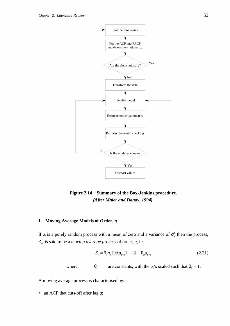
Chapter 2. Literature Review 53
No
No
Yes
Yes
Forecast values
Is the model adequate?
Perform diagnostic checking
Estimate model parameters
Identify model
Transform the data
Are the data stationary?
Plot the ACF and PACF,and determine stationarity
Plot the time series
Figure 2.14 Summary of the Box-Jenkins procedure.
(After Maier and Dandy, 1994).
1. Moving Average Models of Order, q
If at is a purely random process with a mean of zero and a variance of σa2 then the process,
Zt , is said to be a moving average process of order, q, if:
Z a a at t t q t q= + + +− −θ θ θ0 1 1 L (2.31)
where: θi are constants, with the ai’s scaled such that θ0 = 1.
A moving average process is characterised by:
• an ACF that cuts-off after lag q;

54 Chapter 2. Literature Review
• a PACF that dies-down.
The manner in which the PACF dies-down identifies the order of the MA process. For
example:
• First order MA process The PACF dies-down in a damped exponential
decay fashion;
• Second order MA process The PACF dies-down according to a combination
of damped exponential and sine wave decays.
The parameters θ0, θ1, ... , θq , are estimated using a numerical optimisation algorithm such
as a grid search, the Gauss-Newton approach (Cryer, 1986), or the innovations algorithm
(Brockwell and Davis, 1987).
As an example, for the MA(1) case (a first-order moving average process) the parameter,
θ1, and the variance of the white noise, σa2 , are determined by the following relationships:
( )θ
σθ
112
1
2 0
12
1 1 4
2
1
12
=− + −
=+
r
r
ca
(2.32)
2. Autoregressive Models of Order, p
If at is a purely random process with a mean of zero and a variance of σa2 then the process,
Zt , is said to be an autoregressive process of order, p, if:
Z Z Z Z at t t p t p t= + + + +− − −φ φ φ1 1 2 2 L (2.33)
where: φi are constants.
An autoregressive process is characterised by:
• an ACF that dies-down;
• a PACF that cuts-off after lag p.
The manner in which the ACF dies-down identifies the order of the AR process. For
example:

Chapter 2. Literature Review 55
• First order AR process The ACF dies-down in a damped exponential decay
fashion;
• Second order AR process The ACF dies-down according to a combination of
damped exponential and sine wave decays.
Consider an AR process of order m and mean, µ, (Chatfield, 1975):
( ) ( ) ( )Z Z Z Z at t t m t m t− = − + − + + − +− − −µ φ µ φ µ φ µ1 1 2 2 L (2.34)
Given N observations, Z1, Z2, ... , Zn , the parameters, µ, φ1, φ2, ... , φm , can be estimated by
least squares by minimising S, usually called the conditional sum-of-squares function
(Cryer, 1986), where:
( ) ( ) ( )[ ]S Z Z Zt t m t mt m
n
= − − − − − −− −= +∑ µ φ µ φ µ1 1
2
1
L (2.35)
As an example, for the AR(1) case (a first-order autoregressive process) the parameter, φ1,
and the variance of the white noise, σa2 , are determined by the following relationships:
( )φ
σ φ1 1
20 1 11
=
= −
r
c ra
(2.36)
3. Mixed Autoregressive-Moving Average Models of Order, p, q
The mixed autoregressive-moving average process (ARMA) is a useful class of time series
model since a stationary random field can often be described using fewer parameters than a
purely MA or AR process (Chatfield, 1975). An ARMA process of order (p, q) is defined
as:
qtqtttptpttt aaaaZZZZ −−−−−− θ++θ+θ++φ++φ+φ= 22112211 LL (2.37)
An ARMA process is characterised by:
• an ACF that dies-down;
• a PACF that dies-down.
The manner in which the ACF and PACF die-down identifies the order of the ARMA

56 Chapter 2. Literature Review
process. For example:
• ARMA process of order (1, 1) Both the ACF and PACF die-down in a damped
exponential decay fashion.
4. Integrated Mixed Autoregressive-Moving Average Models
Finally, the integrated mixed autoregressive-moving average process (ARIMA) is a class
of time series model that incorporates non-stationary data. The ARIMA process is one
that, after performing several differences, as outlined in §2.5.1.2((ii)), reduces to an ARMA
process (Brockwell and Davis, 1987). If Zt, a non-stationary random field, is differenced
to order d, that is:
W Ztd
t= ∇ (2.38)
such that Wt is a stationary random field, then the ARIMA process is of the form:
qtqtttptpttt aaaaWWWW −−−−−− θ++θ+θ++φ++φ+φ= 22112211 LL (2.39)
If Wt is an ARMA(p, q) process, then Xt is an ARIMA(p, d, q) process. Cryer (1986) stated
that for practical purposes, d is usually taken to 1 (first-difference), or at most 2 (second-
difference).
Estimation of the parameters in both the ARMA and ARIMA models use the same
techniques adopted for the MA and AR models, detailed previously.
(b) Diagnostic Checking
Once a preliminary model has been identified and its associated parameters estimated, a
number of diagnostic checks are available to determine how well the model fits the
observed random field. Each technique analyses the residuals, that is, the differences
between the observations and the fitted values, as well as the autocorrelation coefficient of
the residuals, kr̂ . A brief discussion of the more commonly used techniques follows.
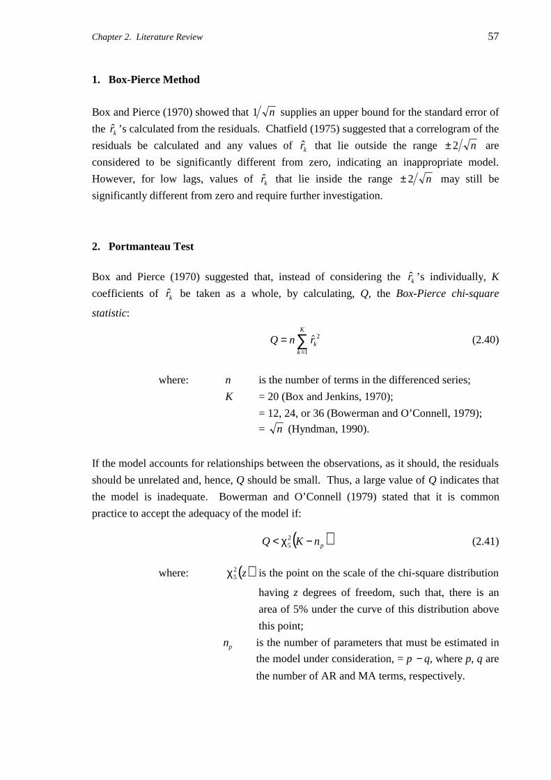
Chapter 2. Literature Review 57
1. Box-Pierce Method
Box and Pierce (1970) showed that 1 n supplies an upper bound for the standard error of
the kr̂ ’s calculated from the residuals. Chatfield (1975) suggested that a correlogram of the
residuals be calculated and any values of kr̂ that lie outside the range ± 2 n are
considered to be significantly different from zero, indicating an inappropriate model.
However, for low lags, values of kr̂ that lie inside the range ± 2 n may still be
significantly different from zero and require further investigation.
2. Portmanteau Test
Box and Pierce (1970) suggested that, instead of considering the kr̂ ’s individually, K
coefficients of kr̂ be taken as a whole, by calculating, Q, the Box-Pierce chi-square
statistic:
Q n rkk
K
==
∑ $ 2
1
(2.40)
where: n is the number of terms in the differenced series;
K = 20 (Box and Jenkins, 1970);
= 12, 24, or 36 (Bowerman and O’Connell, 1979);
= n (Hyndman, 1990).
If the model accounts for relationships between the observations, as it should, the residuals
should be unrelated and, hence, Q should be small. Thus, a large value of Q indicates that
the model is inadequate. Bowerman and O’Connell (1979) stated that it is common
practice to accept the adequacy of the model if:
( )pnKQ −χ< 25 (2.41)
where: ( )z25χ is the point on the scale of the chi-square distribution
having z degrees of freedom, such that, there is an
area of 5% under the curve of this distribution above
this point;
np is the number of parameters that must be estimated in
the model under consideration, = p − q, where p, q are
the number of AR and MA terms, respectively.

58 Chapter 2. Literature Review
Brockwell and Davis (1987, 1991) suggested that the portmanteau test is useful for
disqualifying unsatisfactory models, but often fails to reject poorly fitting models. As a
consequence, Brockwell and Davis (1991) recommended that the portmanteau test should
not be used on its own.
In addition, Brockwell and Davis (1987, 1991) suggested a number of diagnostic tests
which examine the randomness of the residuals. These include: a test based on turning
points; the difference-sign test; and the rank test. However, in the interests of brevity,
these are not treated in this thesis. Further details regarding these tests are given by
Brockwell and Davis (1987, 1991).
(c) Forecasting
Having identified an appropriate model, estimated its parameters and performed diagnostic
checks to confirm its validity, the user is then in a position to employ the model to forecast
future values of the random field, or in terms of the spatial domain, estimate values at
locations other than those measured. In essence, forecasting is one of the primary
objectives of time series analysis. Focusing solely on univariate stochastic processes,
several forecasting techniques have been traditionally applied to time series. These
include: extrapolation of trend curves (regression); exponential smoothing; Holt-Winters
forecasting technique; and the Box-Jenkins approach (Chatfield, 1975). Whilst each of
these methods are frequently applied with good results, the Box-Jenkins methodology,
detailed above and summarised in Figure 2.14, is the most versatile, and provides a more
systematic framework for building, analysing and forecasting with time series models
(Chatfield, 1975; Bowerman and O’Connell, 1979). In addition, the Box-Jenkins
methodology tends to give more accurate forecasts than other methods. On the other hand,
the Box-Jenkins approach suffers from a number of limitations:
• At least 50 to 100 observations are necessary to build a reliable Box-Jenkins model, and
even greater if a seasonal component, or a relationship non-stationarity are present
(Bowerman and O’Connell, 1979). In addition, these authors recommended that,
because of the large amount of data required, the Box-Jenkins methodology is best
suited to time series with small sampling intervals.
• Several ARIMA models may be found to fit the data equally well. While these models
are usually almost equivalent, occasionally each model will generate different forecasts
(Chatfield, 1975).
• There are currently no procedures available for automatically updating the model
parameters as new data are measured. As additional observations are added to the

Chapter 2. Literature Review 59
random field, the complete model-building procedure must be repeated (Bowerman and
O’Connell, 1979).
• The Box-Jenkins procedure is complex, time-consuming and expensive (Chatfield,
1975; Bowerman and O’Connell, 1979).
• Considerable experience is required to identify an appropriate ARIMA model
(Chatfield, 1975).
(vi) Cross-Covariance and the Cross-Correlation Function
Just as the autocovariance and the autocorrelation functions are used to measure
dependencies by comparing a time series with itself at successive lags, it is also possible to
compare two separate time series with each other to calculate positions of strong
correlation. The tools used to do this are the cross-covariance and the cross-correlation
function (CCF). The cross-covariance coefficients, between two time series,
X X X X Xn= 1 2 3, , , ,K and Y Y Y Y Yn= 1 2 3, , , ,K , at lag k, ckXY, are given by (Box and Jenkins,
1970):
( )( )[ ] K ,2 ,1 ,0 E =−−= + kYYXXc kiikXY(2.42)
and the cross-covariance between Y and X at lag k, ckYX, is:
( )( )[ ] K ,2 ,1 ,0 E =−−= + kXXYYc kiikYX(2.43)
where, in general, c ck kXY YX≠ . However, since:
( )( )[ ] ( )( )[ ]c X X Y Y Y Y X X ck i k i i i k kXY YX= − − = − − =− − −E E (2.44)
ckXY need only be calculated for k = 0, ± 1, ± 2, ± ...
Since the time series, X and Y, may be expressed in different units, it is useful to define the
cross-correlation coefficient at lag k, ρkXY, as:
K ,2 ,1 ,0 ±±±=σσ
=ρ kc
YX
kk
XY
XY(2.45)

60 Chapter 2. Literature Review
Again, only estimates can be made of ckXY and ρkXY
, and hence the sample cross-covariance
coefficient at lag k, ckXY
* , and the sample cross-correlation coefficient at lag k, rkXY, are
defined as:
( )( )
( )( )
−−=−−
=−−
=
∑
∑+
=−
−
=+
K
K
,2 ,1 ,0 1
,2 ,1 ,0 1
1
1*
kXXXXn
kXXXXn
ckn
ikii
kn
ikii
kXY (2.46)
rc
s skk
k
X YXY
XY= = ± ± ±*
, , , 0 1 2 K (2.47)
where: sX is the sample standard deviation of X = cXX0
* ;
sY is the sample standard deviation of Y = cYY0
* .
Again, the accuracy of the sample cross-correlation function (CCF), that is the graph of rkXY
against lag, k, is directly related to the number of observations in the time series, n. As for
the sample autocorrelation function, Box and Jenkins (1970) recommended that n be
greater than 50.
Again, Box and Jenkins (1970) recommended that Bartlett’s approximation be used as a
crude check to ascertain whether certain values of the CCF can be regarded as being
effectively equal to zero. The CCF will be used in §5.3.5 to compare series of qc
measurements to fs measurements, to determine the optimal value of the shift distance
mentioned previously in §2.4.4.
2.5.1.3 Geostatistics
The mathematical technique, which is now universally known as geostatistics, was
developed to assist in the estimation of changes in ore grade within a mine, and is largely a
result of the work of Krige (1951) and Matheron (1965). Since its development in the early
1960’s, geostatistics has been applied to many disciplines including: groundwater
hydrology and hydrogeology; surface hydrology; earthquake engineering and seismology;
pollution control; geochemical exploration; and geotechnical engineering. In fact,
geostatistics can be applied to any natural phenomena that are spatially or temporally
associated (Journel and Huijbregts, 1978; Hohn, 1988).

Chapter 2. Literature Review 61
As mentioned previously, geostatistics is based on the regionalised variable, that is, one
that can be represented by random functions, rather than the classical approach which treats
samples as independent random variables. The regionalised variable has properties that are
partly random and partly spatial and has continuity from point to point, however, the
changes are so complex that they cannot be described by a tractable deterministic function
(Davis, 1986).
One of the basic statistical measures of geostatistics is the semivariogram, which is used to
express the rate of change of a regionalised variable along a specific orientation. The
semivariogram is treated below.
(i) Semivariogram
The semivariogram is a measure of the degree of spatial dependence between samples
along a specific orientation, and represents the degree of continuity of the property in
question. The semivariogram, γh , is defined by the following equation:
( )[ ]2E2
1ihih XX −=γ + (2.48)
where: Xi is the value of the property, X, at location, i;
Xi+h is the value of the property, X, at location, i+h;
h is the displacement between the data pairs;
E[…] is the expected value.
Thus, the semivariogram is defined as half the expected value, or mean, of the squared
difference between pairs of points, Xi and Xi+h , separated by a displacement, h. If the
regionalised variable is stationary and normalised to have a mean of zero and a variance of
1.0, the semivariogram is the mirror image of the autocorrelation function, as shown in
Figure 2.15.
Even though a regionalised variable is spatially continuous, like the ACF and PACF, it is
not possible to know its value at all locations. Instead its values can only be determined
from samples taken from a population. Thus, in practice, the semivariogram must be
estimated from the available data, and is generally determined by the following
relationship:
( )∑=
+ −=γN
iihih XX
N 1
2*
2
1(2.49)
where: γ h* is the experimental semivariogram, that is, one based on the
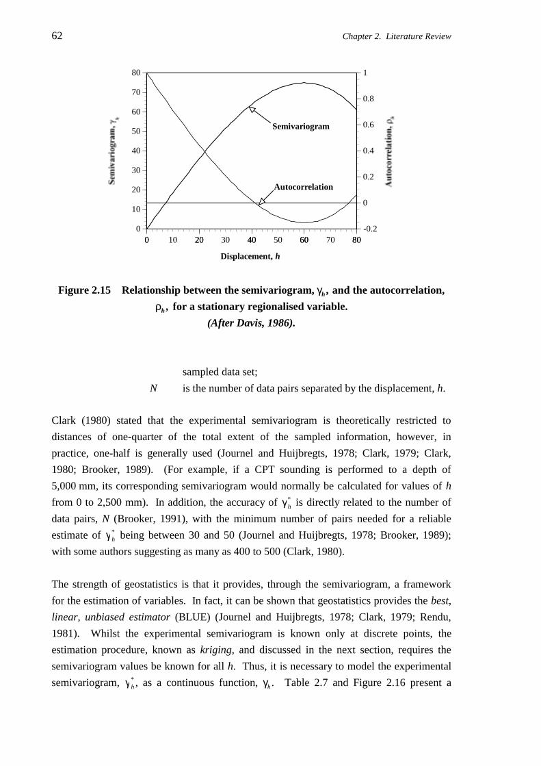
62 Chapter 2. Literature Review
0
10
20
30
40
50
60
70
80
-0.2
0
0.2
0.4
0.6
0.8
1
0 20 40 60 800 10 20 30 40 50 60 70 80
Autocorrelation
Semivariogram
Displacement, h
Figure 2.15 Relationship between the semivariogram, γh , and the autocorrelation,
ρh , for a stationary regionalised variable.
(After Davis, 1986).
sampled data set;
N is the number of data pairs separated by the displacement, h.
Clark (1980) stated that the experimental semivariogram is theoretically restricted to
distances of one-quarter of the total extent of the sampled information, however, in
practice, one-half is generally used (Journel and Huijbregts, 1978; Clark, 1979; Clark,
1980; Brooker, 1989). (For example, if a CPT sounding is performed to a depth of
5,000 mm, its corresponding semivariogram would normally be calculated for values of h
from 0 to 2,500 mm). In addition, the accuracy of γ h* is directly related to the number of
data pairs, N (Brooker, 1991), with the minimum number of pairs needed for a reliable
estimate of γ h* being between 30 and 50 (Journel and Huijbregts, 1978; Brooker, 1989);
with some authors suggesting as many as 400 to 500 (Clark, 1980).
The strength of geostatistics is that it provides, through the semivariogram, a framework
for the estimation of variables. In fact, it can be shown that geostatistics provides the best,
linear, unbiased estimator (BLUE) (Journel and Huijbregts, 1978; Clark, 1979; Rendu,
1981). Whilst the experimental semivariogram is known only at discrete points, the
estimation procedure, known as kriging, and discussed in the next section, requires the
semivariogram values be known for all h. Thus, it is necessary to model the experimental
semivariogram, γ h* , as a continuous function, γh . Table 2.7 and Figure 2.16 present a

Chapter 2. Literature Review 63
Table 2.7 Commonly used model semivariograms.
Model Mathematical Function Remarks
Pure Nugget γ h C= 0 C0 = Nugget
SphericalahCC
ahCa
h
a
hC
h
h
≥+=γ
≤+
−=γ
when
when 22
3
0
03
3
C + C0 = Sill;
Range = a
Exponential ( )γ hh aC e C= − +−1 0 Effective Range = 3a†
Gaussian ( )γ hh aC e C= − +−1
2 2
0 Effective Range = 3a †
Linear γ h ph C= + 0 p = slope
Power γ αh ph C= + 0 0 < α < 2
de Wijsian γ αh h C= +3 0ln( ) α = absolute dispersion
Note: In addition, each of the models, above, obey γ0 = 0.† From Olea (1991).
0
50
100
0 50 100
Spherical
Gaussian
Exponential
Displacement, h
0
50
100
0 50 100
Power
de Wijsian
Linear
Displacement, h
Figure 2.16 Commonly used model semivariograms with C0 set to zero.
number of semivariogram models that are commonly used in the literature, the most widely
applied of these being the spherical model.
With particular reference to the spherical model, three parameters are used:
C0 is defined as the nugget effect and arises from the regionalised variable being
so erratic over a short distance that the semivariogram goes from zero to the
level of the nugget in a distance less than the sampling interval. The nugget
effect is the result of three separate phenomena (Rendu, 1981):

64 Chapter 2. Literature Review
1. microstructures within the geological material - which have been observed
from the study of the spatial variability of mineral concentrations of core
samples. Two adjacent cores will exhibit a nugget effect when one of
them contains a nugget and the other does not (Journel and Huijbregts,
1978). Several researchers have stated that soils also exhibit this
behaviour (Calle et al., 1987; Li and White, 1987a; Soulié et al., 1990;
Jaksa et al., 1993);
2. sampling, or statistical, errors - as will be detailed in §2.5.2.1, C0 depends
greatly on the spacing between individual samples (Brooker, 1977; Journel
and Huijbregts, 1978; Clark, 1979; Clark, 1980; de Marsily, 1982);
3. measurement errors - if it were possible to obtain a repeat measurement at
precisely the same location, the observations would differ by an amount
directly dependent on the measurement technique. Measurement errors are
also manifested by a non-zero value of the semivariogram at zero lag.
It has been standard practice in the treatment of the spatial variability of soils
to attribute the nugget effect solely to measurement errors associated with the
testing method (Baecher, 1986; Wu and El-Jandali, 1985; Filippas et al.,
1988). However, Li and White (1987a) suggested that while some of the
nugget effect can be attributed to measurement errors, the possibility of small-
scale random effects, that is, microstructures, cannot be ignored in
geotechnical properties. The relationship between measurement errors and
the nugget effect will be examined in some detail in §5.5.
C + C0 is known as the sill which measures half the maximum, on average, squared
difference between data pairs.
a is defined as the range of influence, or range, and is the distance at which
samples become independent of one another. Data pairs separated by
distances up to a are correlated, but not beyond.
Clark (1979) described the process of fitting a model to an experimental semivariogram as
essentially a trial-and-error approach, usually achieved by eye. Brooker (1991) suggested
the following technique as a first approximation in determining the appropriate parameters
for a spherical model:
• The experimental semivariogram and variance of the data are plotted;
• The value of the sill, C + C0, is approximately equal to the variance of the data;

Chapter 2. Literature Review 65
• A line is then drawn with the slope of the semivariogram near the origin, which
intersects the sill at two thirds the range, a;
• This line intersects the ordinate at the value of the nugget effect, C0.
In addition, Brooker (1991) stated that the accuracy of the modelling process depends on
both, the number of pairs in the calculation of the experimental semivariogram, and the lag
distance at which it is evaluated.
Journel and Huijbregts (1978) suggested that automatic fitting of models to experimental
semivariograms, such as least squares methods, should be avoided. This is because each
estimator point, γ h* , of an experimental semivariogram is subject to an estimation error and
fluctuation which is related to the number of data pairs associated with that point. Since
the number of pairs varies for each point so, too, does the estimation error. The authors
recommended that the weighting applied to each estimated point, γ h* , should come from a
critical appraisal of the data, and from practical experience.
Similar to the autocorrelation function of random variables, the semivariogram is greatly
facilitated by stationarity, that is, the semivariogram depends only on the separation
distance and not on the locality of the data pairs. The regionalised variable can be regarded
as consisting of two components: the residual and the drift. If a drift, or trend, exists in the
data, which leads to non-stationarity, it must first be removed (Journel and Huijbregts,
1978; Henley, 1981). It has been shown by Davis (1986), that if the drift is subtracted from
the regionalised variable, the residuals will themselves be a regionalised variable and will
have local mean values of zero. In other words, the residuals will be stationary and the
semivariogram can be evaluated.
(ii) Estimation - Kriging
Once the form of the semivariogram is known, it is possible to estimate the values of the
measured parameter at any unsampled location. The estimation procedure is known as
kriging, named after D. G. Krige, a South African mining engineer who pioneered the
application of statistical techniques to the estimation of ore bodies. Kriging essentially
involves the determination of a series of weights, w w w wn1 2 3, , , ,K , that are applied to the
sample data set, Y Y Y Yn1 2 3, , , ,K , to yield a linear estimate, Yp* , at an unsampled location, p,
such that:
nnp YwYwYwYwY ++++= 332211* L (2.50)
and:1 321 =++++ nwwww L (2.51)

66 Chapter 2. Literature Review
It is expected that the estimate, Yp* , will differ from the actual (but unknown) value, Yp , by
an amount known as the estimation error, εp , (the same as the residual used in random field
theory), such that:
ε p p pY Y= −* (2.52)
Provided that no local trend exists within the sample data set, and the weights sum to one,
as indicated by Equation (2.51), the estimate, Yp* , will be unbiased. That is, the average of
the estimation errors will be zero, and linear, since the estimate is a linear combination of
the sample values. The variability of the errors, or the estimation variance, σε2, for the
general linear unbiased estimator can be shown to be equal to (Clark, 1979; Brooker,
1991):
[ ] ),(),(),(21 1 1
2 UUSSwwUSwn
i
n
i
n
jjijiii γ−γ−γ=σ ∑ ∑∑
= = =ε (2.53)
where: γ( , )S Ui is the average value of the semivariogram, γh , as one end of
the vector h is in Si , and the other independently sweeps the
unknown element U;
U is a point, line, area, or block;
γ ( , )S Si j is the average value of the semivariogram between points Si
and Sj;
γ( , )U U is the average of the semivariogram between all pairs of
points within the element U.
For the continuous case, Equation (2.53) can be expressed as:
( ) ( ) ( )⌡⌠
⌡⌠ −γ−⌡
⌠ −γ−−γ=σ ∑∑∑= ==
εUU
N
i
N
jjiji
N
iii dydxyx
Uxxwwdxxxw
U 21 11
2 12(2.54)
By calculating the estimation variance, σε2, it is possible to rank any estimation regime5.
Kriging enables an optimal set of weights, w w w wn1 2 3, , , ,K , to be determined so that σε2
can be minimised. This is achieved by differentiating σε2 with respect to the weights, and
setting this differential equal to zero, as:
5 A methodology used to estimate the value of a domain, based on applying a series of weights, nwwww , ,,, 321 K , to a
set of sample data. Such estimation regimes include: polygonal, inverse distance, and inverse distance squared. Eachof these estimation procedures are examined in §7.4.2.

Chapter 2. Literature Review 67
∂σ∂
ε2
0w
i ni
= = where: 1, 2, 3, , K (2.55)
Solving this equation will yield n-equations and n-unknowns. However, an additional
equation needs to be satisfied so that the estimator will be unbiased; that is, the weights
must sum to equal one:
wii
n
==∑ 1
1
(2.56)
After differentiation, the following system of equations is obtained:
( ) ( )
γ
=
µ
γ
1
,
011
1
,
1
M
M
M
M
L
M USwSS iiji (2.57)
where: µ is the Lagrange multiplier.
This results in n + 1 equations and n + 1 unknowns. In this way, kriging provides the
minimum estimation variance and the best, linear, unbiased estimation (BLUE) regime, as
mentioned previously. The estimation variance associated with kriging, or the kriging
variance, σk2 , can be evaluated using Equation (2.53), or alternatively:
[ ] ( ) ( )σ µγ
γk iiw
S UU U2
1
=
−K K
M
M
,, (2.58)
Brooker (1980) detailed the following key steps involved in the kriging method of
geostatistical estimation:
1. A structural study to determine the semivariogram.
2. Selection of the samples to be used in evaluating the element, U.
3. Calculation of the γ of the kriging system of equations.
4. Solution of the system of equations to obtain the optimal weights.
5. Use of these results to calculate the estimate of U and its associated estimation variance.
Since the geostatistical process of kriging was first formalised in the 1960’s, several
modifications to this process have been proposed by various researchers. These are
generally sub-divided into two forms: linear kriging, and non-linear kriging. These two
forms include:

68 Chapter 2. Literature Review
Linear Kriging:
• ordinary kriging (Isaaks and Srivastava, 1989; Olea, 1991) - the technique defined
previously in §2.5.1.3(ii) simply as ‘kriging’;
• simple kriging (Journel and Huijbregts, 1978; Olea, 1991) - the same as ordinary
kriging, except that the mean is known and, hence, the final row is deleted from all
matrices, as is the final column of the square matrix. Simple kriging is the best of all
minimum mean square error estimators only when a multinormal distribution is used as
a model for the random function (Olea, 1991);
• universal kriging (Journel and Huijbregts, 1978; Rendu, 1981; Olea, 1991) - simple
kriging of the residuals of a regionalised variable after automatically removing optimal
estimates of the drift. It is used for non-stationary data, that is, when a deterministic
trend exists in the measured data.
Non-Linear Kriging:
• disjunctive kriging (Journel and Huijbregts, 1978; Clark, 1979; Olea, 1991) - a
distribution-dependent estimator which is used when a bias exists in the measured data,
and is the most demanding of the kriging procedures in terms of stationarity conditions,
computer resources, and mathematical understanding on the part of the user;
• lognormal kriging (Olea, 1991) - simple kriging or ordinary kriging of a logarithmically
transformed set of observations, having a multivariate lognormal distribution;
• indicator kriging (Journel, 1983; Olea, 1991) - simple kriging or ordinary kriging
applied to indicator data (samples which have been transformed into binary numbers)
sharing the same threshold;
• probability kriging (Olea, 1991) - an enhancement of indicator kriging which also
includes rank order transformations of the original data;
• Bayesian kriging (Kulkarni, 1984; Omre, 1987; Omre and Halvorsen, 1989) - an
enhancement of indicator kriging which is used when a small number of observations is
available, and when significant experience and knowledge about the phenomenon
should be accounted for in the estimation process.
Indicator, probability and Bayesian kriging are methods of non-parametric geostatistics;
that is, a branch of geostatistics which comprises techniques that do not rely on a prior
multivariate distribution hypothesis (Olea, 1991). The geostatistical process of kriging will
be examined in detail in Chapters 5 and 7.

Chapter 2. Literature Review 69
2.5.1.4 Tests for Non-Stationarity
As discussed in the previous sections, the application of both random field theory and
geostatistics is facilitated by stationary data. Various authors have proposed techniques for
ascertaining the stationarity of the data.
Bennett (1979) proposed five methods for the detection of non-stationary data:
1. Eyeballing - Mere inspection of the scatterplots of the data is often sufficient to detect
non-stationarity, as was shown by Figure 2.12. Eyeballing, however, is not sufficient to
detect the form of the trend, nor most cases of non-stationary variance.
2. Histogram plots - A simple, though crude technique, is to split the random field into a
number of subsections and to plot each of their histograms. Comparison of these
histograms enables shifts in the means and variances to be detected.
3. Inspection of the ACF - As discussed previously, several authors (Box and Jenkins,
1970; Chatfield, 1975; Bowerman and O’Connell, 1979; Davis, 1986) have suggested
that a process that is non-stationary in trend, or mean, is indicated by an ACF which
dies-down slowly. Box and Jenkins (1970) suggested that a stationary time series is
observed by a rapidly damping ACF, whilst Bennett (1979) stated that it is difficult to
determine if a slowly dying-down ACF is the result of non-stationarity, or of
autoregressive parameters very close to unity.
4. The number of significant autocorrelations - This method determines the appropriate
degree of differencing necessary to achieve stationarity, and is implicit in the previous
technique described above. As a result, this method should be combined with the
inspection technique (3), above (Bennett, 1979).
5. Significance tests on trends - This technique is applied in four stages:
(i) The trend component, tt, is estimated by least-squares regression;
(ii) The residuals, Et, from this model are calculated and the parameters of an
autoregressive model are estimated, that is:
ptpttt eeee −−− φ++φ+φ= 2211 L (2.59)
(iii) The original data, Xt, are transformed using the estimates of the residual auto-
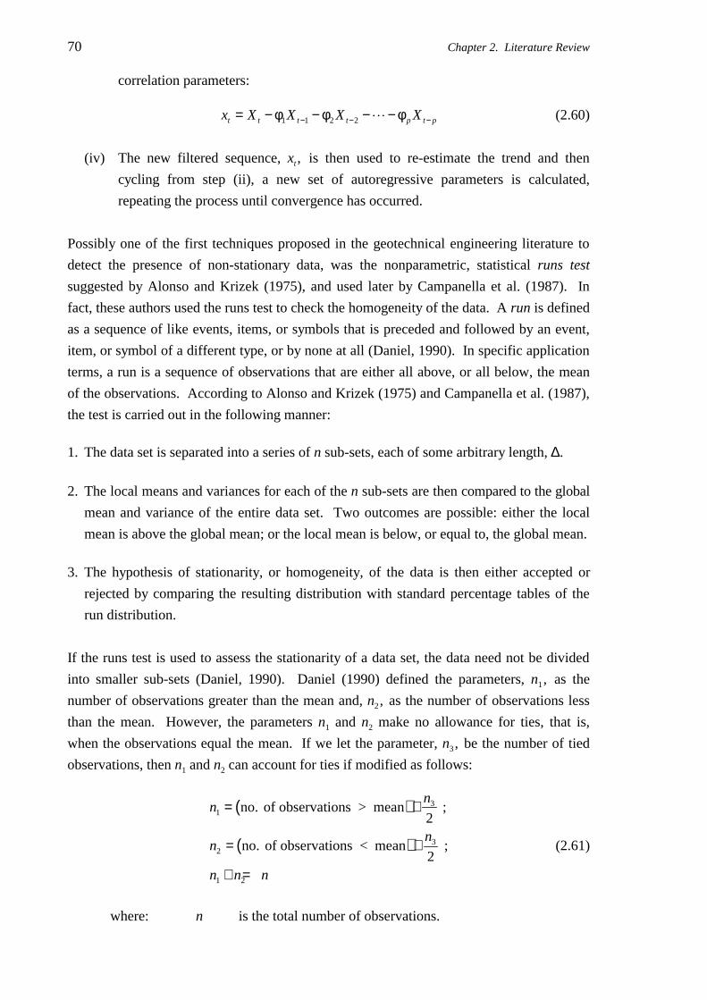
70 Chapter 2. Literature Review
correlation parameters:
ptptttt XXXXx −−− φ−−φ−φ−= 2211 L (2.60)
(iv) The new filtered sequence, xt , is then used to re-estimate the trend and then
cycling from step (ii), a new set of autoregressive parameters is calculated,
repeating the process until convergence has occurred.
Possibly one of the first techniques proposed in the geotechnical engineering literature to
detect the presence of non-stationary data, was the nonparametric, statistical runs test
suggested by Alonso and Krizek (1975), and used later by Campanella et al. (1987). In
fact, these authors used the runs test to check the homogeneity of the data. A run is defined
as a sequence of like events, items, or symbols that is preceded and followed by an event,
item, or symbol of a different type, or by none at all (Daniel, 1990). In specific application
terms, a run is a sequence of observations that are either all above, or all below, the mean
of the observations. According to Alonso and Krizek (1975) and Campanella et al. (1987),
the test is carried out in the following manner:
1. The data set is separated into a series of n sub-sets, each of some arbitrary length, ∆.
2. The local means and variances for each of the n sub-sets are then compared to the global
mean and variance of the entire data set. Two outcomes are possible: either the local
mean is above the global mean; or the local mean is below, or equal to, the global mean.
3. The hypothesis of stationarity, or homogeneity, of the data is then either accepted or
rejected by comparing the resulting distribution with standard percentage tables of the
run distribution.
If the runs test is used to assess the stationarity of a data set, the data need not be divided
into smaller sub-sets (Daniel, 1990). Daniel (1990) defined the parameters, n1, as the
number of observations greater than the mean and, n2, as the number of observations less
than the mean. However, the parameters n1 and n2 make no allowance for ties, that is,
when the observations equal the mean. If we let the parameter, n3, be the number of tied
observations, then n1 and n2 can account for ties if modified as follows:
( )
( )
nn
nn
n n n
13
23
1 2
2
2
= +
= +
+ =
no. of observations > mean ;
no. of observations < mean ; (2.61)
where: n is the total number of observations.

Chapter 2. Literature Review 71
This technique of allowance for ties is similar to that suggested by Noether (1991) for use
with Kendall’s τ test, which is discussed in detail below. The runs test, when used to
assess stationarity of a data set, however, is given by the following steps (Daniel, 1990):
1. The parameters, n1, n2, and n3 are evaluated.
2. The number of runs, R, are calculated.
3. If the data are determined by a random process, that is, a stationary one, then the
calculated number of runs, R, must lie within upper and lower critical bounds, as given
by standard runs test tables, for example Daniel (1990). However, these tables are
generally limited to situations where n ≤ 20. For large values of n, Daniel (1990)
recommended the use of Equation (2.62), where zR is distributed normally, with a mean
of zero and variance of unity. As a consequence, the value of zR can be compared with
values given in standard, normal distribution tables. Hence, if zR ≤ ±1.96, then the data
can be assumed to be stationary with 95% confidence.
( )( ) ( )1
22
12
212
21
212121
21
21
−++−−
++
−=
nnnn
nnnnnn
nn
nnR
zR (2.62)
The runs test, although used by Alonso and Krizek (1975) and Campanella et al. (1987) as
a test for homogeneity, has found little use elsewhere in the geotechnical engineering
literature.
Journel and Huijbregts (1978) suggested that an experimental semivariogram which
increases as rapidly as h 2 for large distances, h, most often indicates the presence of a
trend, and hence non-stationary data. This technique was also proposed by Kulatilake and
Southworth (1987) and Kulatilake and Ghosh (1988) for the detection of non-stationarities
in geotechnical engineering data. This technique is the geostatistical equivalent of the time
series method of a slowly decaying ACF (the third method suggested by Bennett (1990), as
detailed previously).
Ravi (1992) stated that the most powerful test for non-stationarity is Kendall’s τ test. The
test essentially involves the calculation of the test statistic, τ, which measures the
probability of concordance minus the probability of disconcordance (Daniel, 1990). The
observation pairs, (Xi , Yi) and (Xj , Yj), are said to be concordant if the difference between Xi
and Xj is in the same direction as the difference between Yi and Yj . That is, if either Xi > Xj
and Yi > Yj , or Xi < Xj and Yi < Yj , then the pairs are concordant. Discordance, on the other
hand, is when the directions of the differences are not the same. If Xi = Xj and/or Yi = Yj ,
72 Chapter 2. Literature Review
then the pairs are neither concordant nor discordant. The test statistic, τ, is given by
(Daniel, 1990; Noether, 1991):
( )τ =−
S
n n12 1
(2.63)
where: n is the number of pairs of (X, Y) observations.
To obtain S the following process is used:
1. The observations (Xi , Yi) are ranked in a column according to the magnitude of the X’s,
with the smallest X first, through to the largest X last. The X’s are thus arranged in their
natural order.
2. Each Y value is then successively compared with each Y value appearing below it. In
making these comparisons, a pair of Y values, that is, the value of Y in question and the
value of Y below it, is said to be in natural order if the Y below is larger than the Y
above. On the other hand, a pair of Y values is in reverse natural order if the Y below is
smaller than the Y above.
3. The parameter, P, is the number of pairs in natural order, and the parameter, Q, is the
number of pairs in reverse natural order.
4. S is then simply the difference between P and Q, that is, S = P − Q.
The value of Kendall’s τ lies between +1 and −1 with: τ = +1 indicating perfect positive
correlation; τ = −1 indicating perfect negative correlation; and τ = 0 indicating no
correlation. Hence, when applied to the assessment of stationarity, a value of τ close to
zero indicates that the data are stationary, whereas a value of τ near +1 or −1 indicates non-
stationary data. Usually, for some confidence level specified by the user, the value of τ is
compared with critical values of τ tabulated in many statistics texts; for example Daniel
(1990) and Noether (1991). As with the runs test, tables of critical τ values are rarely given
for data sets where n exceeds about 40. For large values of n, Daniel (1990) recommended
the use of the following equation:
( )( )
zn n
nτ
τ=
−+
3 1
2 2 5(2.64)
Again, zτ is normally distributed with a mean of zero and variance of unity and, as a
consequence, the value of zτ can be compared with values given in standard, normal
distribution tables. Hence, if zτ ≤ ±1.96 then the data can be assumed to be stationary with
Chapter 2. Literature Review 73
95% confidence. Additionally, Noether (1991) suggested the use of the parameter, c, given
by:
c =+−
1
1
ττ
(2.65)
The parameter, c, suggests that the probability of concordance, P, is c times more likely
than the probability of disconcordance, Q.
In summary, of the various techniques for assessing data stationarity, as detailed above, it is
generally accepted that none have been found to be entirely suitable on their own. Perhaps
the most suitable and most widely used in the field of geotechnical engineering are:
inspection of a scatterplot of the data; examination of the ACF; inspection of the
experimental semivariogram; the runs test; and Kendall’s τ test. It will be these five
techniques which will be used to assess the stationarity of the data, detailed in Chapter 4,
and examined in Chapter 5.
In the next section treatment will be given to the historical progress of the understanding of
the spatial variability of geotechnical materials. This discussion will focus essentially on
soils, as much work has already been done in the field of rocks, particularly in the
evaluation of ore bodies. Where possible, this treatment follows a chronological sequence.
2.5.2 Historical Studies Concerned with the Spatial Variability ofGeotechnical Materials
The development of the understanding of the spatial variability of soils has evolved along
two, essentially separate streams - one involving random field theory, and the other
focusing on geostatistics. In general, the evolution of each stream has occurred
independent of the other, with a few exceptions. As a result, this treatment of the historical
development of the spatial variability of geotechnical materials will be separated into these
two streams.
Since the very early days of soil mechanics, it was recognised that geotechnical materials
varied from one location to another. Karl Terzaghi, universally regarded as the father of
geotechnical engineering, in his Presidential Address to the First International Conference
on Soil Mechanics and Foundation Engineering in 1936, stated: “...the earth in its natural
state is never uniform” (Terzaghi, 1936). However, it was not until 1966 that this aspect,
that is, the spatial variability of soils, began to be examined rigorously.

74 Chapter 2. Literature Review
2.5.2.1 Random Field Theory
Probably the first detailed investigation of the spatial variability of soils was that by Lumb
(1966), where he examined the statistical properties of London Clay and four Hong Kong
soils, namely: Marine Clay; Alluvial Sandy Clay; Residual Silty Sand; and Residual Clayey
Silt. Lumb (1966) stated that any soil property such as the void ratio, undrained shear
strength, and so on, is generally not constant, but depends on the location of the point
within the soil mass. He stated that the properties can be taken as independent of lateral
position and, at most, linearly dependent on the depth, zk , below the ground surface. Thus,
for a particular soil property, vk , at a point k within a soil mass, Lumb (1966) proposed the
following random variable model:
v a bzk k k= + + ε (2.66)
where: a, b are constants;
zk is the depth of point k below the ground surface;
εk is a random variable at point k with a mean of zero.
In this model, a + bzk accounts for a linear trend of the property, vk , with depth, and εk
represents the random fluctuation of this property about the trend. In addition, Lumb
(1966) suggested that it is occasionally more convenient to express the random variable, εk ,
in the form: εk = σuk , since σ may itself be a function of depth. Lumb (1966) defined the
variable, uk , as a standardised random variable having a mean of zero and a standard
deviation equal to unity. In addition, Lumb (1966) proposed three different cases of the
form of the standard deviation, as shown in Figure 2.17.
•
• ••
•
• •
•••
• •••
••
•
••
•
•
•
•
•
•
Dep
th, z
Soil Parameter, v
Case 1
••
••
•• •
•••
• •
••••
•
••
•
•
•
•
•
•
Dep
th, z
Soil Parameter, v
Case 2
••
••
•• •
•••
• •
••••
•
••
•
•
•
•
•
•
Dep
th, z
Soil Parameter, v
Case 3
•
••
•
•
•
•
• •
•
•
•
••
•
Figure 2.17 Different forms of a soil parameter, v, with depth, z. (After Lumb, 1966).

Chapter 2. Literature Review 75
Case 1 refers to the soil property, v, being normally distributed about the mean value, m,
whereas Case 2 refers to v being normally distributed about a linear trend, a + bz, and, in
both cases, the variance is independent of depth. Case 3 represents the situation where v is
normally distributed about a linear trend, a + bz, and the variance increases with depth. By
plotting the standardised random variable, u, against the standardised normal variate, ζ(Pearson and Hartley, 1956), and applying the χ2 test to a combination of vane shear and
carefully sampled, unconfined compression test results, Lumb (1966) was able to show that
the undrained shear strength, su , and drained internal angle of friction, φd , of the three soils
follow normal distributions, and possess statistical properties which are summarised in
Table 2.8. In addition, Lumb (1966) suggested that a rational choice of design parameter
can be made from the mean, or linear trend provided that the form of the variance is
known. As can be seen from Table 2.8, the spatial variability models, represented by the
mean linear trends, provide relatively basic models of the variability structure of these
geotechnical properties.
Table 2.8 Summary of statistical properties. (After Lumb, 1966).
Soil Property Mean, m Std. Deviation, σ Coeff. of Variation, CV
Marine Clay su (kPa) 1.04z + 1.89 0.19z + 0.35 18.4% (3)*
London Clay su (kPa) 22.1z 3.58z 16.2% (3)
Silty Sand tanφd 0.692 0.0958 13.8% (1)Note: z is the depth below the ground surface in metres;
* (1) and (3) refer to the cases shown in Figure 2.17.
Hooper and Butler (1966) presented the results of a large number of undrained triaxial tests
performed on undisturbed samples of London Clay, and also found that the undrained shear
strength follows a normal distribution.
Lumb and Holt (1968) examined undrained shear strength results obtained from vane shear
tests; and unconfined compression tests, carried out on remoulded and high quality
undisturbed specimens of the soft Marine Clay of Hong Kong. The results, combined from
approximately 100 boreholes, indicated Case 3 behaviour with a high degree of scatter
about the linear trend. From 270 test results, the authors suggested a CV of at least 20%,
and the best linear relationship for the mean value to be:
s zu = ± +( . )1.012 0 1.85012 (2.67)
where: su is the undrained shear strength, in kPa;
z is the depth below the ground surface, in metres.

76 Chapter 2. Literature Review
Again, the use of a linear trend to depict the variability of su represents a relatively
elementary model. Agterberg (1970), for probably the first time, summarised the use of the
autocorrelation function (ACF) with respect to geotechnical engineering materials; in his
case, rocks. Based on a general model:
v t sk k k k= + + ε (2.68)
where: vk is the value of a parameter v in a random field at
location k;
tk is the trend component at k, which expresses the global
systematic change and any test method bias;
sk is the signal component at k, which expresses the local
correlated portion of the spatial variation;
εk is the random uncorrelated portion.
Agterberg (1970) proposed the following procedure for estimating the ACF:
1. Eliminate spatial heteroscedasticity from the data, if present, by data transformation.
2. Estimate the trend by fitting deterministic functions by the method of least squares.
3. Remove the trend component from the data; the remaining data being the residuals.
4. Estimate the ACF of the residuals.
5. Fit a model to the ACF of the residuals.
Agterberg suggested that the ACF for a continuous random variable is exponential. By
analysing elevations of the surface of a geological stratum from 200 boreholes, Agterberg
(1970) concluded that the best results can be obtained by first fitting a low degree trend
function (e.g. a quadratic) and using an estimation procedure based on the residuals.
While Lumb (1966) stated that soil properties can be regarded as laterally independent,
Lumb (1974) later acknowledged lateral dependence, in addition to depth dependence.
Lumb (1974) re-examined the results of Lumb and Holt (1968) and, for probably the first
time in the geotechnical engineering literature, used the ACF to investigate the spatial
dependence of soil properties by making use of the work of Agterberg (1970). Lumb
(1974) suggested that soil properties which are depth dependent generally follow a first
order autoregressive model, also known as a unilateral Markov process, as shown in
Equation (2.69) in the backward direction, and Equation (2.70) in the forward direction.
On the other hand, Lumb (1974) stated that laterally dependent soil properties usually
follow a bilateral Markov process; that is, one with dependence extending in both
directions, as shown in Equation (2.71).

Chapter 2. Literature Review 77
v vk k k= +−φ ε1 1 (2.69)
v vk k k= ++φ ε1 1 (2.70)
v v vk k k k= + +− +φ φ ε1 1 2 1 (2.71)
where: φ1, φ2 are constants generally less than 1.
Lumb (1974) stated that the ACF for the unilateral and bilateral Markov processes are,
respectively, of the following form:
ρ αk
ke= − (2.72)
ρ β βk k K k= ( ) ( )1 (2.73)
where: α, β are constants;
k is the distance, in metres;
K1(x) is the modified Bessel function of the second kind
and first order.
Lumb (1974) went on to fit these models to sample ACFs produced from data obtained
from various sources, and concluded that:
• The lateral variation of the liquid limit of the Bear Paw Shale (a clay shale from
Saskatchewan, Canada) followed satisfactorily a combination of a white noise process
and a bilateral Markov process:
ρk k K k= 0 42 144 1441. ( . ) ( . ) (2.74)
• The lateral variation of the modulus of subgrade reaction of a fine dry sand fill could be
satisfactorily represented, again, by a combination of a white noise process and a
bilateral Markov process, via:
ρk k K k= 059 6 35 6 351. ( . ) ( . ) (2.75)
• The variation with depth of the liquid limit, natural moisture content and the submerged
unit weight of the Hong Kong Marine Clay (Lumb and Holt, 1968) followed a unilateral
Markov process:
ρkke= −1 23. (2.76)
78 Chapter 2. Literature Review
• The variation of the undrained shear strength with depth of the Hong Kong Marine Clay
could be modelled using either a white noise process, or a unilateral Markov process:
ρkke= −0 33. (2.77)
From the results of these analyses, Lumb (1974) stated that the spatial autocorrelations for
the Bear Paw Shale and the Marine Clay were not particularly large, the converse of what
would have been expected for these very uniform deposits. On this basis, and from the
limited data available, Lumb (1974) concluded that no great error would be made in
assuming the properties to be uncorrelated for spacings of the order of 1 to 2 metres.
Wu (1974) also used the ACF to study the spatial correlation of the undrained shear
strength of the soils, in his case, the Chicago Clay. Positive correlation was found to occur
within a vertical distance of 0.9 metres, which is equal to the approximate thickness of the
different geological units within the Chicago area. In addition, Wu (1974) approximated
the ACF by the following relationship:
ρkke= −0 234. (2.78)
Lumb (1975) re-examined the results presented by Lumb (1974) using first- and second-
differences, the ACF, and the partial autocorrelation function (PACF). Lumb (1975) found
that, in all cases, no more than a first-difference was necessary to minimise the variance of
the population; implying that a linear trend component was always sufficient. Since the
soils that he examined showed weak autocorrelations, Lumb (1975) concluded that the
autocovariances and autocorrelations could be neglected and, as a result, their omission
should produce no serious error in the design predictions. This conclusion, in particular,
will be examined in greater detail later in this thesis, with reference to the measured CPT
values of Keswick Clay6.
Diaz Padilla and Vanmarcke (1974) proposed a property, the correlation distance, vo ,
which expresses the extent of spatial variation of some parameter, v. The authors defined
vo as the distance required for the ACF to decay from 1 to e−1 (0.3679). Diaz Padilla and
Vanmarcke (1974) suggested that vo be determined by fitting the following exponential
decay models to the sample ACF:
( )ρ∆∆
zz ve= − 0 (2.79)
6 Lumb (1975) also made reference to the spectral density function (SDF); that is, the Fourier transform of the ACF; as
an additional spatial variability descriptor. Lumb suggested that there are some theoretical advantages in using afrequency domain, instead of the more natural distance domain. However, since the vast majority of research reportedin the geotechnical engineering literature has focused on the distance domain, the theory associated with the SDF willnot be applied in the present study. A detailed treatment of the analysis of properties in the frequency domain; that is,spectral analysis; is given by Vanmarcke (1983).

Chapter 2. Literature Review 79
( )ρ∆∆
zz ve= − 0
2
(2.80)
where: ∆z is the spacing between samples.
Using these relationships, Diaz Padilla and Vanmarcke (1974) were able to calculate
vertical correlation distances for the moisture content, void ratio and preconsolidation
pressure of a soft organic, silty clay from California, as 1.5, 1.5, and 0.3 metres,
respectively. In addition, the authors found that the horizontal correlation distance of the
preconsolidation pressure of this clay was of the order of 90 metres. However, Diaz
Padilla and Vanmarcke (1974) commented that, since the smallest lateral spacing between
boreholes was 90 metres, they could not detect smaller scale correlation effects. The
usefulness of the parameter, vo , was not emphasised until Vanmarcke (1977a) presented his
treatment of random field theory, which is discussed below.
Matsuo and Asaoka (1977) compared the undrained shear strengths of many undisturbed
samples of a normally consolidated Japanese marine clay, obtained from unconsolidated
undrained triaxial tests. While extending the number of cases proposed by Lumb (1966)
from three to ten, the authors found that the results fell into Lumb’s Case 3, and a small
number into Case 2. Matsuo and Asaoka (1977) concluded that it was difficult to
determine the exact spatial autocorrelation of su because of sample disturbance. In
addition, the authors found that significant autocorrelation of su in the vertical direction
usually occurs within a distance of 1.5 metres.
Vanmarcke (1977a, 1977b, 1978, 1983, 1984) provided a major contribution to the study of
spatial variability of geotechnical materials by the use of random field theory. Vanmarcke
(1977a) stated that, in order to describe a soil property, v, stochastically, three parameters
are needed: (i) the mean, m; (ii) the standard deviation, σ (or the variance, σ2, or the
coefficient of variation, CV); and (iii) the scale of fluctuation, δv. He introduced the new
parameter, δv, which accounts for the distance within which the soil property, v, shows
relatively strong correlation, or persistence, from point-to-point. Furthermore, when the
property is plotted as a function of distance, the scale of fluctuation is closely related to the
average distance between intersections, or crossings, of v and m. Small values of δv imply
rapid fluctuations about the mean, whereas large values suggest a slowly varying property,
with respect to the average. While δv is closely related to the correlation distance, vo (Diaz
Padilla and Vanmarcke, 1974), Vanmarcke (1977a) recommended the use of δv.
Vanmarcke (1983) suggested that δv has an important property, namely:
∫ ∫+∞
∆
+∞
∞− ∆∆ρ=∆ρ=δ
0)(2)( zdzd
zzv (2.81)

80 Chapter 2. Literature Review
That is, the scale of fluctuation, δv , is the area beneath the entire ACF, or twice the area
beneath the positive part of the ACF. To be more specific than Vanmarcke (1977a), with
regard to the three parameters needed to stochastically model a soil profile, in order to
describe a random field in terms of first- and second-order moments, one must quantify the
mean or trend function, the variance, and the correlation structure. As suggested by
Vanmarcke (1977a), the variance of the soil profile may be expressed by σ, CV, or the
variance, σ2, itself. Whilst Vanmarcke (1977a) argued that δv is a simple characterisation
of the correlation structure, as in fact it is, the autocovariance function, ACVF, spectral
density function, SDF, and the variance function, may also be used as descriptors of the
correlation structure. The variance function, Γ ∆v z2 ( ), proposed by Vanmarcke (1977a),
measures the point variance under local averaging, and its value is bounded by 0 and 1.
The variance function is a particularly useful relationship, since it implies that the
variability of spatial averages is lower than the point values. This results from the fact that
fluctuations of v are smoothed in the averaging process. Vanmarcke (1977a, 1983) defined
the standard reduction factor, Γ ∆v z( ) , as the square root of Γ ∆v z2 ( ), and by the following
relationship:
Γ ∆ ∆v
zz( ) =σσ
(2.82)
where: σ∆z is the standard deviation of v spatially averaged over a
depth interval, ∆z;
σ is the standard deviation of the point values of v.
Or, in terms of volume averages:
ΓvVV( ) =
σσ
(2.83)
where: σV is the standard deviation of v spatially averaged over a
volume, V.
In addition, Vanmarcke (1977a) defined the scale of fluctuation, δv , in terms of Γ ∆v z2 ( ), as:
δv v z z= Γ ∆ ∆2 ( ) (2.84)
which is valid when ∆z becomes large.
Vanmarcke (1977a) proposed that the variance function may be represented by:
Model 1:
δ≥∆∆δ
δ≤∆=∆Γ
vv
v
vz
z
zz
for
for 1)(2 (2.85)
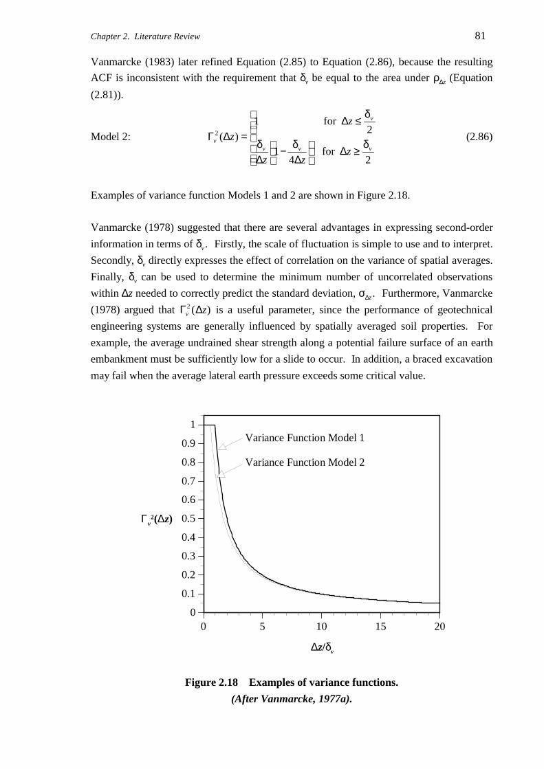
Chapter 2. Literature Review 81
Vanmarcke (1983) later refined Equation (2.85) to Equation (2.86), because the resulting
ACF is inconsistent with the requirement that δv be equal to the area under ρ∆z (Equation
(2.81)).
Model 2:
δ≥∆
∆δ−
∆δ
δ≤∆=∆Γ
2for
41
2for 1
)(2
vvv
v
v
zzz
z
z (2.86)
Examples of variance function Models 1 and 2 are shown in Figure 2.18.
Vanmarcke (1978) suggested that there are several advantages in expressing second-order
information in terms of δv . Firstly, the scale of fluctuation is simple to use and to interpret.
Secondly, δv directly expresses the effect of correlation on the variance of spatial averages.
Finally, δv can be used to determine the minimum number of uncorrelated observations
within ∆z needed to correctly predict the standard deviation, σ∆z . Furthermore, Vanmarcke
(1978) argued that Γ ∆v z2 ( ) is a useful parameter, since the performance of geotechnical
engineering systems are generally influenced by spatially averaged soil properties. For
example, the average undrained shear strength along a potential failure surface of an earth
embankment must be sufficiently low for a slide to occur. In addition, a braced excavation
may fail when the average lateral earth pressure exceeds some critical value.
0
0.1
0.2
0.3
0.4
0.5
0.6
0.7
0.8
0.9
1
0 5 10 15 20
Γv2(∆z)
∆z/δv
Variance Function Model 1
Variance Function Model 2
Figure 2.18 Examples of variance functions.
(After Vanmarcke, 1977a).

82 Chapter 2. Literature Review
Vanmarcke (1977a, 1978 and 1983) proposed a number of methods for estimating the scale
of fluctuation, δv , with particular reference to CPT data. In each of these methods,
Vanmarcke used statistically homogeneous data, that is, the n-dimensional equivalent of
1D stationarity. Vanmarcke (1977a) suggested that statistical homogeneity could be
obtained by standardising the data by means of the following relationship:
v zv z v
sv
( )( )
=−
σ(2.87)
where: vs(z) is the standardised data;
v is the mean of v(z);
σv is the standard deviation of v(z).
Vanmarcke (1983) later recognised that, in some instances, a further transformation, such
as the logarithmic variance transformation (discussed previously in §2.5.1.2(ii)), may be
needed to obtain homogeneity. The more relevant techniques for estimating δv are
presented below.
1. Variance function method for estimating δv
Vanmarcke (1977a) suggested that, firstly, the mean, v , and standard deviation, σv, of
the measured point values are determined. Adjacent observations are then averaged
pairwise, and standard deviation of the resulting spatial averages are calculated. This
yields an estimate of σvΓ(2). This result is plotted on a standard reduction factor graph,
Γ(n) versus n, which is similar in nature to that shown in Figure 2.18. (The parameter,
n, denotes the number of adjacent observations of v which are averaged). Subsequently,
for each value of n, the standard deviation of the spatial averages is computed, and Γ(n)
evaluated by dividing the result by σ. Vanmarcke (1977a) suggested that the predicted
values of Γ(n) will approach the theoretical values given by:
Γ∆
( )nn z
v=δ
0
(2.88)
where: ∆z0 is the sampling interval.
Finally, δv is estimated by fixing n, observing Γ(n), and substituting into:
δv n n z= Γ ∆20( ) (2.89)

Chapter 2. Literature Review 83
2. Autocorrelation function method for estimating δv
Vanmarcke (1978, 1983) and Li and White (1987a) proposed that δv could be evaluated
from the ACF by the relationships shown in Table 2.9. As a result, δv may be estimated
by fitting one of the ACF models to the sample ACF by using standard curve fitting
techniques, such as ordinary least squares.
Table 2.9 Theoretical autocorrelation functions used to determine the scale of
fluctuation, δv . (After Vanmarcke, 1977a, 1983; Li and White, 1987a).
ModelNo.
AutocorrelationFunction
Model(Process)
Scale ofFluctuation, δv
1
≥∆
≤∆∆
−=ρ∆
az
aza
z
z
for 0
,for 1 Triangular model a
2 ρ∆∆
zz be= − Simple Exponential, AR(1) 2b
3( )2cz
z e ∆−∆ =ρ
Squared Exponential, orGaussian, model
π c
4
∆+=ρ ∆−
∆ d
ze dz
z 1 AR(2) 4d
5 ( )α∆=ρ α∆−∆ ze z
z cos Cosine Exponential αNote: AR(1) is a first-order, autoregressive process;
AR(2) is a second-order, autoregressive process.
3. Mean-crossings approximation of δv
An alternative technique, proposed by Vanmarcke (1977a), is to use the approximate
relationship:
dv v v≈ ≈π
δ δ2
1.25 (2.90)
where: dv is the average distance between the intersections of
the fluctuating property, v(z), and its mean, v .
Since the introduction of these techniques, the ACF method appears to be the most widely
adopted in the geotechnical engineering community, with the variance function method
being somewhat less popular. This is possibly due to the fact that the variance function
84 Chapter 2. Literature Review
method involves a degree of subjectivity with regard to the choice of the number of
observations, n, whereas the ACF method is somewhat less subjective. The latter,
however, implicitly assigns equal weighting to each autocorrelation coefficient. This is
slightly erroneous, since more data pairs contribute to the coefficients at lower lags than
those at higher lags. However, this effect becomes somewhat negligible when the number
of data pairs is large.
Vanmarcke (1977b) applied the theory of random fields to earth slopes in an attempt to
make reliable forecasts of slope failure events. He used data obtained from the site
investigation of the failure of a 6.5 metre high, and 100 metre long, embankment in a deep
deposit of varved clay in Ontario, Canada (Lacasse and Ladd, 1973). Based on
measurements of su obtained from vane shear tests performed in a number of vertical
boreholes, Vanmarcke (1977b) calculated the vertical scale of fluctuation, δV, to be
5 metres, and the horizontal scale of fluctuation, δH , to be 46 metres. Vanmarcke (1977b),
however, gave no information regarding the number and spacing of the data used in the
calculation of δV and δH . Furthermore, no details were provided with respect to
transformations, if any, that were performed on the data. Vanmarcke (1977b) subsequently
used these values to estimate the probability of failure of the slope. Most importantly,
however, Vanmarcke (1977b) provided a theoretical framework for the three-dimensional
probabilistic analysis of the classical, limit-equilibrium, slope stability problem.
Since its introduction, several researchers have applied random field theory to the stability
analysis of slopes (Anderson et al., 1984; Li and White, 1987b; Li and Lumb, 1987;
Bergado and How, 1991; Mostyn and Soo, 1992), as well as other geotechnical problems
(Baker, 1984; Tang and Sidi, 1984; Baker and Zeitoun, 1987; Vanmarcke, 1987;
Vanmarcke, 1989; Cherubini and Garrasi, 1991; Ditlevsen and Gluver, 1991; Fenton and
Vanmarcke, 1991; Bergado et al., 1992). Random field theory, as applied to slope stability
analyses, will be examined in Chapter 8.
Based on the work of Vanmarcke (1977a, 1977b, 1978 and 1983), several researchers have
since estimated the ACF and the scale of fluctuation, δv , of several geotechnical properties
of many different soil types. Their results are summarised in Table 2.10.
The relationships between the scale of fluctuation, δv , and the correlation distance, vo , for
each model given in Table 2.9, are summarised in Table 2.11.
Baecher et al. (1980) and DeGroot and Baecher (1993) defined the correlation distance as
the distance at which the autocovariance function decays to e−1, not the ACF, as defined by
Diaz Padilla and Vanmarcke (1974). However, this is not a generally accepted definition

Chapter 2. L
iterature Review
85
Table 2.10 Autocorrelation functions, correlation distances and scales of fluctuations given by various researchers.
(Adapted from Li and White, 1987a).
SoilType
GeotechnicalProperty
Direction(H: Horizontal,
V: Vertical)
TestType*
AutocorrelationFunction
ρz
CorrelationDistance
vo (m)
Scale ofFluctuation
δv (m)
SamplingInterval∆z0 (m)
Researcher(s)
Bear Paw Shale Liquid Limit, wL H - 0.605zK1(1.44)z ≈ 0 ≈ 0 0.15
Hong Kong Index Properties V - e−1.23z 0.8 1.6 0.3 Lumb (1974)
Marine Clay su V TUC e−0.33z 3.0 6.0 0.3
Moisture Content, w V - e−0.66z 1.5 3.0 1.5
Soft Organic Silty Clay, Void ratio, e V - e−0.66z 1.5 3.0 1.5 Diaz Padilla and
California Preconsolidation V - e−3.3z 0.3 0.6 1.5 Vanmarcke (1974)
Pressure, σ’p H - e−0.011z 90 180 90
Chicago Clay su V e−0.234z 4.3 8.6 ? Wu (1974)
Bear Paw Shale Liquid Limit, wL H - 0.445zK1(1.31)z ≈ 0 ≈ 0 0.15 Lumb (1975)
Fine Dry Sand Fill Subgrade Modulus H PLT e−6.1z 0.16 0.33 0.1
Soft Clay, Louisiana γ V - ? 1.2 ? ? Vanmarcke and Fuleihan (1975)
Clean Sand, qc V CPT e−0.9z 1.1 2.22 0.2
Florida fs V CPT e−1.6z 0.6 1.25 0.2
Clay qc V CPT e−1.91zcos(2.62z) 0.5 ? 0.05
Soft Silty Loam, Moisture Content, w ? - e−0.16zcos(0.3z) 6.3 ? 0.5 Alonso and Krizek (1975)
Coast of the Liquid Limit, wL ? - e−0.23zcos(0.31z) 4.3 ? 0.5
Ariake Sea, Void ratio, e ? - e−0.191zcos(0.31z) 5.2 ? 0.5
Japan Bulk unit weight, γ ? - e−0.253zcos(0.41z) 4.0 ? 0.5
Note: * : Abbreviations for test types are given in the Glossary. continued on the following pages...

86 C
hapter 2. Literature R
eview
Table 2.10 Autocorrelation functions, correlation distances and scales of fluctuations given by various researchers. (...continued).
(Adapted from Li and White, 1987a).
SoilType
GeotechnicalProperty
Direction(H: Horizontal,
V: Vertical)
TestType*
AutocorrelationFunction
ρz
CorrelationDistance
vo (m)
Scale ofFluctuation
δv (m)
SamplingInterval∆z0 (m)
Researcher(s)
Marine Clay,Japan
su V TUU e−αz
α = 0.75 - 1.60.6 - 1.3 1.3 - 2.7 1.0 - 7.7 Matsuo (1976)
New Liskeard Varved su V VST ? ? 5 ≈ 1.5 Vanmarcke (1977b) and
Clay, Canada su H VST ? ? 46 ≈ 25 Lacasse and Ladd (1973)
D10 to D90 V - e−0.33z 3.0 6.1 1.5
Sand H - e−0.041z 24 49 61 Fardis (1979)
Deposit ln(RD) V SPT e−0.547z 1.8 3.7 1.5
H SPT e−0.030z 34 67 61
Seabed Deposits, Nth. Sea qc H CPT ( )e z− 302
30 53 > 20 Tang (1979)
Coastal Sand qc ? CPT ? 5 ? ?
Compacted γd V - ? 5 ? ? Baecher et al. (1980)
Clay γd H - ? 5 ? ?
Dune Sand SPT-N ? SPT ? 20 ? ?
Hydraulic H - ? ? ≈ 3.5 1.52 - 3.0
Pleistocene Conductivity V - ? ? ≈ 1.7 1.52 - 3.0
Quadra Sand, Porosity H - ? ? ≈ 3.3 1.52 - 3.0 Smith (1981)
Vancouver, Canada V - ? ? ≈ 6.5 1.52 - 3.0
D50 V - ? ? ≈ 0.9 1.52 - 3.0
Note: * : Abbreviations for test types are given in the Glossary. continued on the following page...

Chapter 2. L
iterature Review
87
Table 2.10 Autocorrelation functions, correlation distances and scales of fluctuations given by various researchers. (...continued).
(Adapted from Li and White, 1987a).
SoilType
GeotechnicalProperty
Direction(H: Horizontal,
V: Vertical)
TestType*
AutocorrelationFunction
ρz
CorrelationDistance
vo (m)
Scale ofFluctuation
δv (m)
SamplingInterval∆z0 (m)
Researcher(s)
Sand ln(RD) V SPT e−0.547z 1.8 3.7 1.5 Fardis and Veneziano (1981)
Deposit H SPT e−0.030z 34 67 61
Soft Clay, su V VST e−0.826z 1.2 2.4 1.0 - 3.3 Asaoka and A-Grivas (1982)
New York su V VST e−0.322z 3.1 6.2 3.0 - 4.8
Alluvial Deposits,Spain
1 qc V CPT e−αz
α = 0.78 - 23.10.04 - 1.3 0.09 - 2.6 0.05 Ximenez de Embun & Romana
(1983)
Soft Glacial Clay, su V TUC ? 1.0 ? 0.4
North Sea su V VST ? 1.0 ? 0.4 Wu and El-Jandali (1985)
Fine Silty Sand, Nth. Sea qc V CPT ? 1.4 ? 0.2
Deltaic Soils, Canada qc V CPT e−1.18zcos(2.63z) 0.85 0.13 - 0.71 0.025 Campanella et al. (1987)
Silty Clay, California qc V CPT e−2.94z 0.34 0.68 0.1 Spry et al. (1988)
Various, California Permeability H/V - ? - δH / δV ≈ 40 - Fenton and Vanmarcke (1991)
Silty Clays,
Bangkok
Embankment
Settlement
V - e−αz
α = 0.5 - 2.00.5 - 2.0 1.0 - 4.0 > 1 Bergado and How (1991)
Silty Clay qc V CPT e−10z 0.1 0.2 0.020 Li and Lee (1991)
qc V CPT ? ? 0.24 - 0.32 0.025 Wickremesinghe
Deltaic Soils, Canada fs V CPT ? ? 0.35 - 0.40 0.025 and
Pore Pressure, ubt V CPT ? ? 0.14 - 0.42 0.025 Campanella (1993)
Note: * : Abbreviations for test types are given in the Glossary.

88 Chapter 2. Literature Review
Table 2.11 Relationship between the scale of fluctuation, δv , and the correlation
distance, vo , for various ACF models.
ModelNo.
AutocorrelationFunction
Scale ofFluctuation, δv
vo
vδ
1
≥∆
≤∆∆
−=ρ∆
az
aza
z
z
for 0
,for 1 a † 1
2 ρ∆∆
zz be= − 2b † 1
2
3 ( )2czz e ∆−
∆ =ρ π c † 1
π
4
∆+=ρ ∆−
∆ d
ze dz
z 1 4d † 1
4
5 ( )α∆=ρ α∆−∆ ze z
z cos α ‡ 1
Note: † from Vanmarcke (1983);‡ from Vanmarcke (1978).
of vo and, as a result, the interpretation suggested by Diaz Padilla and Vanmarcke (1974)
and Vanmarcke and Fuleihan (1975) will be used. While some authors use the correlation
distance (Baecher et al., 1980; Li and White, 1987a; DeGroot and Baecher, 1993) to
express the autocorrelation of geotechnical properties, the majority of researchers use the
scale of fluctuation, δv .
Asaoka and A-Grivas (1982) presented the results of 56 field vane shear tests performed on
a saturated, soft, organic, silty clay from New York, obtained from four separate vertical
boreholes, A1, A2, B1 and B2. The tests were nominally spaced at 1.0 metre intervals, but
varied between 0.85 and 1.25 metres. Asaoka and A-Grivas (1982) normalised the
measurements of su , with respect to depth, z, by introducing the parameter, ui , which they
defined as:
us
zi
u
i
i= (2.91)
where: suiis the undrained shear strength of sample i;
zi is the depth below ground of the ith sample.
Asaoka and A-Grivas (1982) modelled the variability of the undrained shear strength by

Chapter 2. Literature Review 89
means of the straight line function:
s zu =−β
β0
11(2.92)
where: su is the mean estimate of the undrained shear strength;
β β0 1, are parameters obtained from ordinary least squares,
OLS, such that: u ui i i= + +−β β ε0 1 1 ;
εi is an error term, with zero mean and constant
variance.
The authors found that for the four boreholes su varied between 1.50z and 2.49z, with a CV
of between 17.8% and 30.2%. However, because the spatial variability was modelled by
means of a straight line, the function given in Equation (2.92) provides a relatively poor fit
of the actual measured variability, as shown in Figure 2.19. In addition, the model
proposed by Asaoka and A-Grivas (1982) makes no allowance for irregularly spaced data
and, as has been pointed out above, the data from each of the boreholes were not sampled
at regular intervals.
0
0
0
0
0
0
0
0
0
0
0
0
0
0
0
0
0
0
0
0
0
30
25
20
15
10
5
0 10 20 30 40 50 60 70 80
0 Measured data
Asaoka & A-Grivas (1982)
Undrained Shear Strength, su (kPa)
Figure 2.19 Spatial variability model of su at borehole A1.
(After Asaoka and A-Grivas, 1982).
90 Chapter 2. Literature Review
Using random field theory, Baecher (1982) proposed a useful method for separating the
scatter observed in geotechnical data into its two component sources: the spatial variability
of the material; and the random measurement error associated with the test itself. Baecher
(1982) suggested, as did Agterberg (1970) and Lumb (1974) before him, that the spatial
variation of some parameter, vx , at a location x within a soil mass, may be treated as a
combination of a deterministic component, as well as a stochastic, or random, component,
as shown in the following equation:
vx = tx + ξx (2.93)
where: tx is the trend component at location x, usually determined
by OLS regression;
ξx is the random perturbation from the trend at x.
In addition, Baecher (1982) suggested that the random measurement error is presumed to
be independent from one test to another, to have zero mean, and to have constant variance.
As a consequence, the measurement, mvx, of the parameter, vx , may be expressed as:
m tv x x xx= + +ξ ζ (2.94)
where: ζx is the random measurement error at x.
After some algebraic manipulation, Baecher (1982, 1986) stated that the autocovariance,
ck mv( ), of the measurement, mv , at lag, k, may be shown to equal:
c c ck k kmv v( ) ( ) ( )= +
ζ(2.95)
where: ck v( )is the autocovariance function (ACVF) of v at lag, k;
ck( )ζis the autocovariance function of the random
measurement error, ζ, at lag, k.
A similar relationship can be derived that incorporates the ACF, rather than the ACVF.
Baecher (1982, 1986) proposed that, since ck( )ζ is equal to the variance of ζ at k = 0, and
ck( )ζ is equal to zero at k ≠ 0, the random measurement error may be determined by
extrapolating the observed ACVF, or ACF, back to the origin, as shown in Figures 2.20
and 2.21.
Baecher (1986) stated that, by using this method, typical in situ measurements of soils have
been found to contribute random measurement errors anywhere between 0% and 70% of
the data scatter. It will be shown in §5.5 that Baecher’s approach suffers from a number of
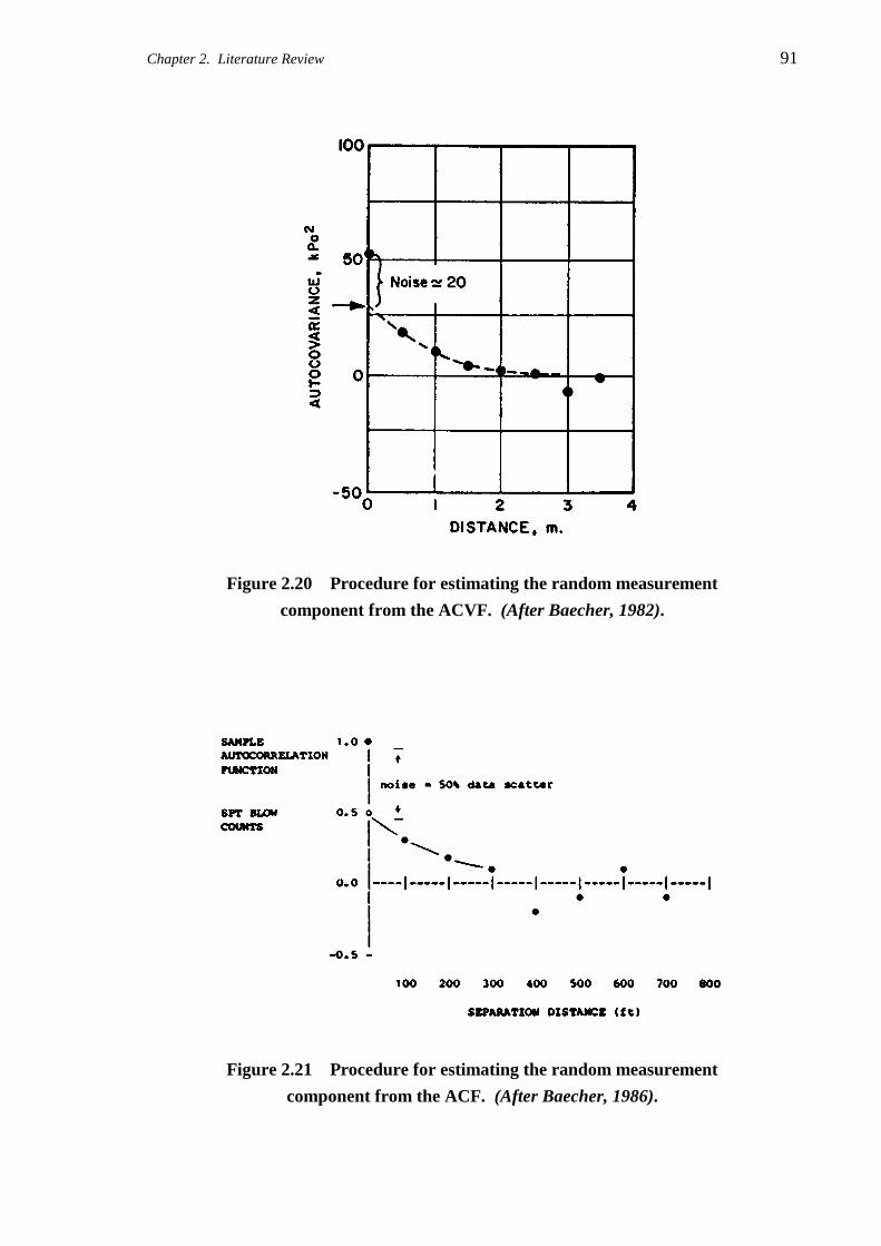
Chapter 2. Literature Review 91
Figure 2.20 Procedure for estimating the random measurement
component from the ACVF. (After Baecher, 1982).
Figure 2.21 Procedure for estimating the random measurement
component from the ACF. (After Baecher, 1986).

92 Chapter 2. Literature Review
limitations. As a consequence, the technique should be used with care, and with attention
given to the factors discussed in §5.5.
Wu and El-Jandali (1985) suggested a slightly different technique to Baecher’s for
estimating the random measurement error associated with geotechnical testing. Wu and El-
Jandali proposed a method which incorporates time series analysis and, in particular, the
Box-Jenkins methodology, and accounts for the random testing error by including an error
term, εt, in the ARMA model, as shown in the following equation:
tqtqtttptpttt aaaaZZZZ ε+θ−−θ−θ−+φ++φ+φ= −−−−−− 22112211 LL (2.96)
Wu and El-Jandali (1985) proposed the parameter, PRE, the percentage random testing
error, and expressed it as:
PRE e
z
= ×σσ
2
2 100% (2.97)
where: σe2 is the variance of the random testing error;
σz2 is the variance of the observed, or transformed, data.
The technique proposed by Wu and El-Jandali (1985) essentially involves fitting an
ARMA model to the observed or transformed data (or an ARIMA model to the differenced
data) and calculating σe2 by substituting into Equation (2.98). Since σz
2 is equal to the
autocovariance at lag 0, that is c0, PRE can be directly obtained by substituting into
Equation (2.97).
( ) ( ) 21
2110 1 ezaqzaapp qccccc σ+−θ−−−θ−σ+φ++φ= LL (2.98)
where: cza(−k) ( )= −φ θ σk k a2 ;
φi are coefficients of the AR process;
θi are coefficients of the MA process.
Using this technique, Wu and El-Jandali (1985) found that:
• unconfined compression tests performed on Oslo clay were best represented by an
ARMA(1,3) model, and that the percentage random testing error, PRE, was found to
equal 54.9%, as compared with 24% using Baecher’s technique;
• undrained shear strengths obtained from field vane tests in Oslo clay were best
represented by an MA(2) model, and PRE was found to equal 5.7%, as compared with
5% using the method proposed by Baecher (1982);

Chapter 2. Literature Review 93
• measurements of qc obtained from a typical cone penetration test in sand were best
modelled using an ARIMA(0,1,1), and PRE was found to equal 6.2%, as compared
with 0% using Baecher’s technique.
Kulatilake and Varatharajah (1986) proposed a weighted regression approach to model and
estimate the trend component of geotechnical properties in one dimension. The technique,
used to transform heteroscedastic data to satisfy stationarity, applies a series of weights to
the covariance matrix of the residuals in an iterative fashion. Using mechanical cone
penetrometer data performed in Florida sands, from Schmertmann (1969), Kulatilake and
Varatharajah (1986) found that a fourth-order polynomial best fitted the data and that
weighted regression was not needed, since the data exhibited constant variance with depth.
Kulatilake and Southworth (1987) extended this work and proposed a technique for the
estimation of the spatial variability of geotechnical properties in one dimension, based on
random field theory. Their method is summarised in Figure 2.22. Again using the data
reported by Schmertmann (1969), Kulatilake and Southworth (1987) found that an
ARMA(6,1) process best represented the residual data. In addition, the authors
recommended that the semivariogram be used as a check of the stationarity of the data.
Kulatilake and Southworth suggested that stationary data are indicated by an experimental
semivariogram which is modelled using a transitive semivariogram function; that is, one
with a finite sill7.
Kulatilake and Ghosh (1988) later formalised this indirect test for data stationarity, and
Kulatilake and Miller (1987) extended the theoretical framework to incorporate three
dimensions. The technique involves: the estimation of the trend component by fitting a
polynomial surface by OLS regression; transformation of the data by removing the trend
surface; evaluation of the ACF of the residuals; and, finally, estimation by means of the
geostatistical process of kriging. It is evident from this that the technique proposed by
Kulatilake and Miller (1987) makes use of various aspects proposed by others, such as
Agterberg (1970), Asaoka and A-Grivas (1982), and Wu and El-Jandali (1985). However,
the procedure uses the geostatistical estimation technique of kriging and, as such, is a
hybrid method incorporating aspects of both random field theory and geostatistics.
Kulatilake (1989) applied this three-dimensional estimation technique to potentiometric
data from the Wolfcamp aquifer in Texas. He was able to demonstrate the usefulness of
his estimation framework and showed that the estimates, generated by including a
stationary stochastic component, were superior to those obtained using the more common
deterministic approach.
7 In a formal sense, however, stationary data may also be represented by a non-transitive model semivariogram, for
example, a linear semivariogram.

94 Chapter 2. Literature Review
Are the raw datanon-stationary?
Yes
No
No
No
No
Yes
Determine the variances of the meanestimations.
Determine mean estimations.
Is the ARMA modeladequate?
Use diagnostic checks to determinewhether the model is adequate.
Estimate the model coefficients.
Identify a potential ARMA model.
Use Box-Jenkins methodology to modelthe stationary stochastic portion.
Stationary stochastic portioncontains only noise.
Yes
Yes
Is autocorrelationsignificant?
Calculate autocorrelationcoefficients using
normalised residuals.
Calculate autocorrelationcoefficients for raw data.
Are the normalisedresiduals non-stationary?
Perform polynomial regression analysis on rawdata to model the trend. Remove the trend fromthe raw data and obtain the normalised residuals.
Figure 2.22 Estimation technique proposed by Kulatilake and Southworth (1987).
Chapter 2. Literature Review 95
Sulikowska et al. (1991) examined the results of relative density, RD, data obtained from
45 replicate CPTs performed in sand. The authors indicated that the measurement error
associated with the testing was relatively small, with a variance of RD of 0.002298.
However, Sulikowska et al. (1991) gave no indication of the conditions under which the
tests were performed, no global mean, nor any details regarding the sampling interval. As
a consequence, without this additional information, it is difficult to compare the variance
with other similar results. In addition, the authors used random field theory to model the
spatial variability of the data and, subsequently, concluded that the data were best modelled
by an AR(2), or an ARMA(2,2) process.
Ravi (1992) re-examined the data presented by Asaoka and A-Grivas (1982) using the
Box-Jenkins methodology. Instead of normalising the measurements of su with respect to
depth, as suggested by Asaoka and A-Grivas (1982), Ravi (1992) used the standard Box-
Jenkins approach of classical decomposition of the data by removing both a linear, and a
quadratic, trend by means of OLS, as suggested by others before him (Agterberg, 1970;
Asaoka and A-Grivas, 1982; Wu and El-Jandali, 1985; Kulatilake and Ghosh, 1988). In
this manner, Ravi (1992) found that an AR(1) model best fitted the residual data and that,
in all but one of the boreholes, removing the OLS quadratic trend provided a better
representation of the measured data than that obtained by removing the OLS linear trend.
Using the sum of the squares of the difference between the measurements and the
estimated values, Ravi (1992) was able to demonstrate that the standard Box-Jenkins
approach provided a better model of the spatial variability of the undrained shear strength
than the technique proposed by Asaoka and A-Grivas (1982). In addition, Ravi used
Kendall’s τ test to assess the stationarity of the residuals and concluded that, in all cases,
the removal of a linear or quadratic trend provided stationary data. On the other hand, the
technique of normalising with respect to depth, as proposed by Asaoka and A-Grivas
(1982), did not always provide stationary data. Some of Ravi’s results will be re-examined
in Chapter 5, in order to provide a check of the numerical procedures contained within
computer software, specifically written to perform random field theory and geostatistical
analyses presented therein.
The foregoing treatment of random field theory, as applied to the field of geotechnical
engineering, has demonstrated its usefulness as a tool for characterising the spatial
variability of soils and rocks, as well as providing a framework for the estimation of
properties at unsampled locations. While much research effort has been directed towards
the application of random field theory in the field of geotechnical engineering, it has been
almost exclusively applied to one-dimensional situations. Two- and three-dimensional
random field theory frameworks have been suggested (Lumb, 1974; Li and White, 1987a;
Kulatilake and Ghosh, 1988), but no such field studies have yet been published. In

96 Chapter 2. Literature Review
addition, it is evident from the literature that the vast majority of spatial variability studies
have been based on limited data, and on data obtained at relatively large sample spacings.
The following sub-section examines the historical development and application of
geostatistics to the field of geotechnical engineering.
2.5.2.2 Geostatistical Analyses
The study of the spatial variability of soil properties by means of geostatistics has found far
less use in the geotechnical community than that using random field theory. Over the last 5
to 10 years, there has been a growing number of researchers who are directing their efforts
towards the field of geostatistics. While a number of researchers have suggested that
geostatistics is a useful tool in the field of geotechnical engineering, many have relied on
scant or fictitious data (Bogárdi et al., 1983; Nguyen and Baafi, 1986; Ims and Toolan,
1988). This section, however, examines the more significant contributions made with
respect to the application of geostatistics to the study of the spatial variability of soil
properties, and again follows a chronological sequence where possible.
Perhaps the first application of geostatistics to the study of the spatial variability of
geotechnical properties was made by Soulié et al. (1983). In their paper, Soulié et al.
(1983) examined the results of 371 in situ compaction tests which were performed during
the construction of an earth dam, and the locations of which were randomly selected in
three dimensions. Because the data were spatially sparse, 1 test every 3,500 m3, the authors
used a temporal scale rather than a spatial one; that is, the data were sorted according to
their date of testing, rather than their location. The authors then generated an experimental
semivariogram and used this as a basis for ordinary kriging. The kriged estimates were
then used to assess the efficiency of the control testing, the probability of whether further
compaction was necessary or not, and the probability of whether any incorrect decisions
were made. The authors concluded that the application of geostatistics to this kind of
geotechnical problem was very useful. However, the results are questionable because of
the sparsity of the data, and the fact that a temporal scale was used instead of a spatial one.
Soulié (1984) presented the results of 12 CPTs performed in alluvial deposits of sand and
gravel in the Mississippi River flood plain, in the state of Missouri. Measurements of qc
were recorded at vertical intervals of 12.5 mm. The vertical experimental semivariograms
of these data indicated: no nugget, and hence no random measurement error; a periodicity
of 1.5 metres, which the authors attributed to sample disturbance due to a reaming process
which was performed at 1.5 metre intervals in order to reduce lateral stresses on the drilling
rods; and a sill value, C, of 13 MPa2 and a range, a, of 1.2 metres.

Chapter 2. Literature Review 97
In addition, Soulié (1984) and Soulié et al. (1990) presented the results of about 300 field
vane shear tests (VSTs), performed in an intact clay within the James Bay area of Québec,
Canada. Though not expressly stated, the tests appear to have been spaced at vertical
intervals of 0.5 metres, and at irregular horizontal spacings of greater than one metre.
Examination of the vertical VSTs indicated no definite trend with depth and, as a result, the
authors performed no transformation of the data. The vertical semivariograms indicated a
sill of 50 kPa2 and a range, a, of 3 metres; whereas one horizontal semivariogram exhibited
pure nugget behaviour, and another indicated a sill of 25 kPa2 and a range, a, of 7 metres.
In order to account for a measurement bias which was found to exist within the data, the
authors performed a shift of 8 kPa to the su profiles; and the resulting horizontal
semivariogram indicated a sill of 50 kPa2 and a range of 30 metres, with each point on the
semivariogram being represented by generally less than 30 data pairs. While the authors
could not isolate the cause of this bias, it is likely that, since the tests were obtained from
four separate investigations which were carried out over a 3 year period, equipment,
operator, or environmental effects may have influenced the measurements.
By examination of the experimental semivariograms, Soulié et al. (1990) found the
measurement errors to be extremely small and, as a result, they excluded a measurement
error term, and hence a nugget effect, from their spatial variability model. The authors then
used the experimental semivariograms and the spatial variability model to perform ordinary
kriging and presented a cross-sectional elevation, contour plot of estimates of su. Soulié
(1984) and Soulié et al. (1990) were able to demonstrate the value of geostatistics as a tool
for site characterisation and quantifying the spatial variability of the undrained shear
strength of clay soils.
Baecher (1984), on the other hand, presented a number of reasons why geostatistics should
be treated with caution when applied to geotechnical engineering situations. Baecher
(1984) identified three aspects where traditional geotechnical reliability, statistical data
analysis and geostatistics differ.
1. For geotechnical applications, population sizes are often small and, as a consequence,
statistical estimation error plays an important role in geotechnical reliability.
2. The characterisation of soil or rock properties for geotechnical reliability serves as input
to complicated, and often non-linear, numerical transformations, rather than being an
end in itself.
3. While average soil or rock properties, throughout a deposit, are often of interest to
geotechnical problems, just as often it is the geological detail, or extremes, which
control the performance of geotechnical facilities.

98 Chapter 2. Literature Review
While agreeing that the work presented by Soulié (1984) was a valid and useful application
of geostatistics to the field of geotechnical engineering, Baecher (1984) recommended that
its use should be tempered with caution, particularly in relation to the three aspects listed
above. However, the three factors which Baecher (1984) identified apply not only to
geostatistics, but also to random field theory. While Baecher expressed some reservations
in regard to geostatistics, he offered no alternative technique for estimating the spatial
variability of geotechnical materials.
A number of other researchers have applied geostatistics to the study of various
geotechnical engineering parameters, and these are summarised in Table 2.12. In addition,
several researchers have used kriging to estimate and characterise various properties of
soils and rock. These are summarised below.
• Oullet et al. (1987) performed 3D ordinary kriging in order to estimate the modulus of
rigidity of a Colorado rock mass. The authors found that the geostatistical analysis
yielded different results to those reported in a former study, which were obtained using
conventional contouring techniques. As a consequence, Oullet et al. (1987) questioned
the results of the former study.
• Nowatzki et al. (1989) used 2D indicator kriging to predict the occurrence of collapsing
soils in the Tucson area of Arizona. Data were obtained from job files, from a number
of consulting firms, from 411 separate locations yielding 992 data measurements. The
authors found that the theory of geostatistics could be applied successfully to
geotechnical engineering problems where large amounts of reliable data are available.
• Soulié et al. (1990) estimated the undrained shear strength of an intact marine clay,
using 2D ordinary kriging. The authors concluded that the power of geostatistics was
made very apparent by the estimation of values where no measurements were taken,
with the semivariogram enabling local estimations to be made.
• Nobre and Sykes (1992) used 2D universal kriging and Bayesian kriging to estimate the
elevation of bedrock near Lake Erie in Ontario. Universal and Bayesian kriging were
used, in contrast to ordinary kriging, because of the presence of a significant trend in the
bedrock elevations. The authors found that the estimates from both the universal
kriging and Bayesian kriging methods were superior to those obtained by ordinary
kriging. In addition, Nobre and Sykes (1992) suggested that Bayesian kriging is
particularly useful when only a small number of observations are available, and when
significant experience and knowledge can be added to the estimation process.
• Brooker et al. (1995) performed 2D ordinary kriging in order to estimate values of

Chapter 2. L
iterature Review
99
Table 2.12 Model semivariograms and their parameters as given by various researchers.
SoilType
GeotechnicalProperty
Direction(H: Horizontal,
V: Vertical)
TestType*
ModelSemivariogram
γh
ModelParameters
NuggetEffect
C0
SamplingInterval∆z0 (m)
Researcher(s)
Sand & Gravel, Missouri qc V CPT Spherical a = 1.2 m, C = 13 MPa2 0 0.0125 Soulié (1984)
Sandy Clay, qc V CPT Spherical a = 0.6 m, C = 1.0 MPa2 0 0.1 Azzouz et al. (1987) and
France qc H CPT Spherical a = 25 m, C = 0.44 MPa2 0.42 1 and 5 Azzouz & Bacconnet (1991)
Rock, Colorado Modulus of Rigidity V & H CSMD Spherical a = 3 m, C = 92 GPa2 20 0.3 Oullet et al. (1987)
Intact Marine Clay, su V VST Spherical a = 3 m, C = 50 kPa2 0 ≈ 0.5 Soulié et al. (1990)
James Bay, Québec su H VST Spherical a = 30 m, C = 50 kPa2 0 > 1
Alluvial Clay, su V TUC Spherical a = 6.5 m, C = 125 kPa2 0 ≈ 0.5 Honjo and Kuroda (1991)
North of Tokyo su H TUC Spherical a = 200 m, C = 125 kPa2 0 40
Sands and Clays,
Riverland,
Readily Available
Water (RAW)†
H - Spherical a = 200 to 650 m,
C = 130 mm2
100
75 × 75 Brooker et al. (1995)
South Australia Topsoil Depth H - Spherical a = 220 to 1,000 m,
C = 2950 cm2
600 grid
Lightly Over- qc Piezo- a = 2 m, C = 5,400 kPa2 0
consolidated, fs V cone Spherical a = 2 m, C = 4.6 kPa2 0 < 2 cm Chiasson et al. (1995)
Highly Sensitive Clay, Porewater Pressure a = 2 m, C = 1,180 kPa2 0
Montréal, Canada su V VST Spherical a = 2 m, C = 24 - 27 kPa2 0 0.5 m
Note: * : Abbreviations for test types are given in the Glossary.† : An irrigation/soil science parameter which measures the water reservoir of the soil between full point, −8 kPa, and refill point, −60 kPa, and is expressed in mm.

100 Chapter 2. Literature Review
readily available water, RAW, and topsoil depth. The authors concluded that
geostatistical analyses were valuable adjuncts to the more traditional information
available to irrigation system designers.
• Chiasson et al. (1995) used geostatistics to characterise the spatial variability of a lightly
overconsolidated and highly sensitive clay. The study was based on measurements
obtained from piezocone and vane shear tests (VSTs) which were observed to increase
linearly with depth. The authors found that the results of the piezocone and VSTs
yielded the same spatial covariance and statistical distribution, indicating that the
assessed variability is independent of the mode of operation of the testing device. In
addition, Chiasson et al. (1995) found that the piezocone and the VST exhibited no
measurement error.
As can be seen from the treatment of geostatistical analyses in the field of geotechnical
engineering, given above, geostatistics is particularly useful as a technique for
characterising the spatial variability of soils and rocks, and also provides a framework for
the estimation of parameters at locations where no measurements are available.
Furthermore, there has been relatively little research directed towards the application of
geostatistics to the assessment of the spatial variability of soils, when compared to that
relating to random field theory.
2.6 SUMMARY
It is evident from the foregoing treatment of the available literature, that both random field
theory and geostatistics provide adequate frameworks for quantifying and estimating the
spatial variability of geotechnical engineering properties. In addition, it has been
demonstrated that the vast majority of analyses using these two techniques have been based
on limited data, and on data obtained at relatively large sample spacings. This is
particularly so in studies dealing with the lateral variability of geotechnical properties. As
mentioned previously, one of the aims of this research is to obtain a large quantity of
accurate and closely-spaced data on which subsequent spatial variability analyses will be
based.
Furthermore, it has been demonstrated that the CPT provides the facility to measure and
record accurate and reliable data, and possesses the lowest level of measurement error of
any commonly-used in situ test procedure; provided that the equipment is well-maintained
and well-calibrated. The following chapter details a micro-computer based data acquisition
system which was developed in order to provide an accurate, reliable and efficient means
by which to measure and store these CPT data.

101
Chapter Three
Development of a Micro-Computer BasedData Acquisition System for the ConePenetration Test
3.1 INTRODUCTION
This section describes the design, development, calibration and use of a micro-computer
based data acquisition system for the CPT. The system was developed by the author in
order to obtain accurate and reliable, closely-spaced data for subsequent spatial variability
analyses.
3.2 EXISTING DATA ACQUISITION SYSTEMS
As discussed in §2.4.1, the electric cone penetrometer was first developed in Holland in
1965. At that time, measurements of cone tip resistance, qc, and sleeve friction, fs , were
recorded using analogue instruments. De Ruiter (1971) detailed one of the first data
acquisition systems as consisting of a Wheatstone bridge instrument which recorded load
variations directly onto a continuous chart. Depth of the cone penetrometer was measured
by a magnetic reduction coupling installed between the loading frame, which was
connected to the push rods, and the transport mechanism of the chart recorder. In this way,
the chart paper advanced 10 mm for every metre of cone penetration.
Analogue systems, such as the one described by de Ruiter (1971), have several limitations.
These include:
• Scaling is Required to Determine Numerical Values - Since data are stored solely on the
chart plots, should data manipulation and calculation be required, (as is the case with the

102 Chapter 3. Development of a Micro-Computer Based Data Acquisition System for the CPT
evaluation of the friction ratio and the undrained shear strength of the soil), this is only
possible once the data have been scaled from the plots and re-input into a computer or
calculator. This results in: inefficiencies, both from a time and economic perspective;
and inaccuracies from the scaling process itself.
• Stiction and Overshoot - Pen-based chart recorders are affected by: stiction - the friction
developed between the pen and the paper, resulting in delayed response of the chart
recorder; and overshoot - the amount of over-, or under- measurement as a result of the
pen assembly having a finite inertia. These effects combine to reduce the accuracy of
the qc and fs plots.
• Limitations of Thermal Paper - While thermal paper chart recorders can overcome the
effects of stiction and overshoot, the quality of their output deteriorates with exposure to
ultra-violet light. As a result, care needs to be taken when operating these chart
recorders in bright field situations. In addition, the quality of thermal paper deteriorates
with time resulting in a loss of resolution in the qc and fs plots.
In order to overcome these limitations modern CPT data acquisition systems are based on
digital computers. Jamiolkowski et al. (1985) suggested that the potential of the CPT has
been greatly improved by recent advances in data acquisition systems.
De Ruiter (1981, 1982) described a system, used by Fugro Consultants International Pty.
Ltd. in Holland, designed to produce precise data with a high degree of resolution, which is
shown in Figure 3.1. De Ruiter (1981, 1982) stated that the most important part of the data
acquisition system is the signal conditioner, to which all major elements are connected.
The conditioning unit supplies the excitation voltages for the penetrometer, and amplifies
the returned signal to useable and calibrated levels. In addition, it receives pulses from a
rotary encoder which measures depth of the cone penetrometer. These pulses, 1,000 per
metre, are used to control chart displacement, and to trigger a digital data-logger. The
system uses an analogue chart recorder, in addition to the digital acquisition system, to
verify equipment operation and to allow on-site evaluation of the CPT.
Currently, there are a limited number of data acquisition systems that are commercially
available for the CPT. However, those that can be purchased are generally:
• Spacing of measured data may not suit spatial variability research - As discussed
previously, studies focusing on spatial variability require large amounts of relatively
closely-spaced data. Many of the data acquisition systems commercially available
record data at spacings not ideal for this research.
• Expensive - Their cost is generally prohibitive to research projects with limited budgets.

Chapter 3. Development of a Micro-Computer Based Data Acquisition System for the CPT 103
Figure 3.1 Fugro Consultants International Pty. Ltd. data acquisition system.
(After de Ruiter, 1982).
• Difficult to modify - Often the design and details of the elements of the data acquisition
system are not supplied. Consequently the individual components are difficult to modify
to suit requirements that may arise in research. In addition, maintenance of the system
is made more difficult because of the unavailability of these design specifications.
• Errors and limitations of the system and individual components are uncertain - Since
the design details are generally not supplied with the system, any errors, limitations, or
uncertainties associated with the elements of the system are difficult to identify and
quantify.
Due to the limitations of commercially available data acquisition systems for the CPT, it
was decided to design and develop a system at the University of Adelaide, primarily suited
to the investigation of spatial variability of soils. In addition, the Department of Civil and
Environmental Engineering at the University of Adelaide uses the CPT for consulting
projects and, as a result, the data acquisition system should also meet the criteria necessary
for this type of work.
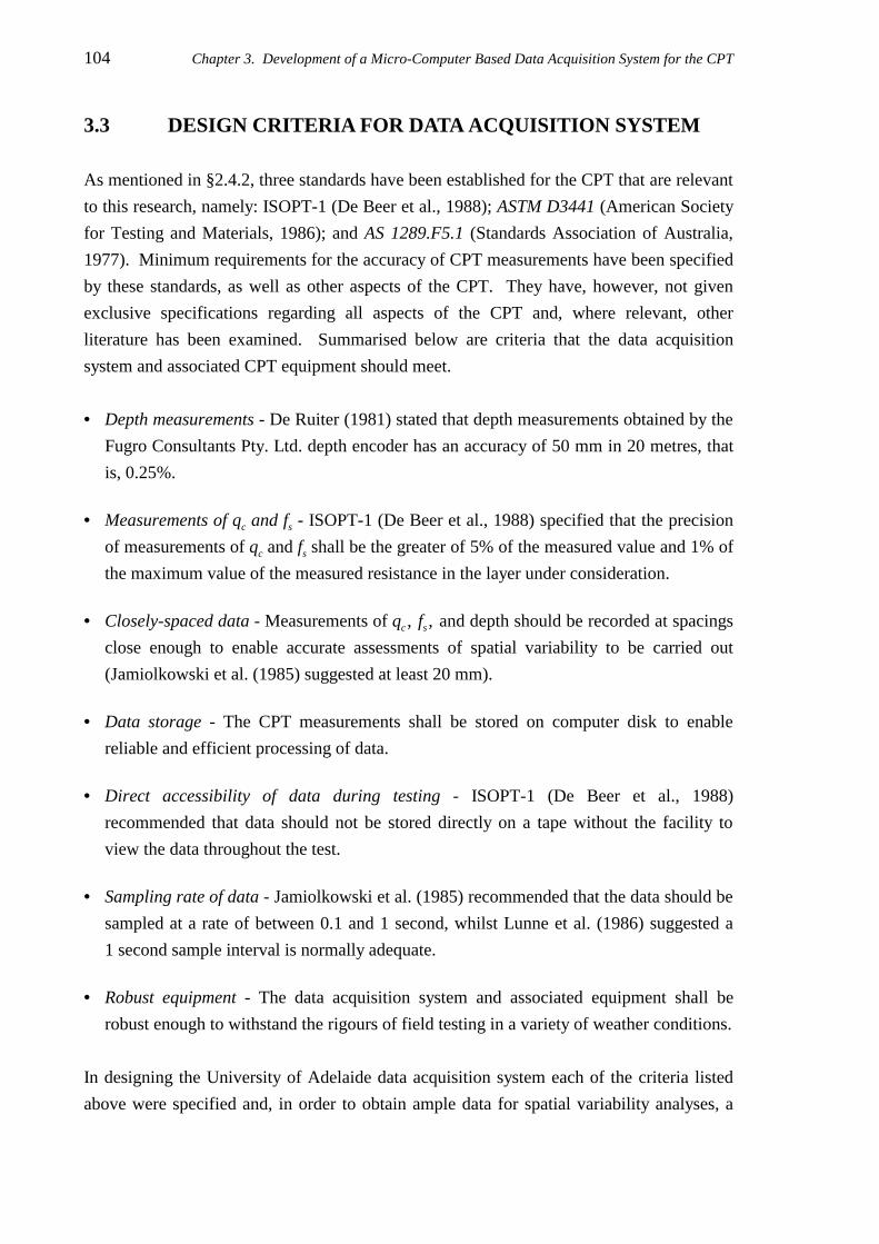
104 Chapter 3. Development of a Micro-Computer Based Data Acquisition System for the CPT
3.3 DESIGN CRITERIA FOR DATA ACQUISITION SYSTEM
As mentioned in §2.4.2, three standards have been established for the CPT that are relevant
to this research, namely: ISOPT-1 (De Beer et al., 1988); ASTM D3441 (American Society
for Testing and Materials, 1986); and AS 1289.F5.1 (Standards Association of Australia,
1977). Minimum requirements for the accuracy of CPT measurements have been specified
by these standards, as well as other aspects of the CPT. They have, however, not given
exclusive specifications regarding all aspects of the CPT and, where relevant, other
literature has been examined. Summarised below are criteria that the data acquisition
system and associated CPT equipment should meet.
• Depth measurements - De Ruiter (1981) stated that depth measurements obtained by the
Fugro Consultants Pty. Ltd. depth encoder has an accuracy of 50 mm in 20 metres, that
is, 0.25%.
• Measurements of qc and fs - ISOPT-1 (De Beer et al., 1988) specified that the precision
of measurements of qc and fs shall be the greater of 5% of the measured value and 1% of
the maximum value of the measured resistance in the layer under consideration.
• Closely-spaced data - Measurements of qc, fs , and depth should be recorded at spacings
close enough to enable accurate assessments of spatial variability to be carried out
(Jamiolkowski et al. (1985) suggested at least 20 mm).
• Data storage - The CPT measurements shall be stored on computer disk to enable
reliable and efficient processing of data.
• Direct accessibility of data during testing - ISOPT-1 (De Beer et al., 1988)
recommended that data should not be stored directly on a tape without the facility to
view the data throughout the test.
• Sampling rate of data - Jamiolkowski et al. (1985) recommended that the data should be
sampled at a rate of between 0.1 and 1 second, whilst Lunne et al. (1986) suggested a
1 second sample interval is normally adequate.
• Robust equipment - The data acquisition system and associated equipment shall be
robust enough to withstand the rigours of field testing in a variety of weather conditions.
In designing the University of Adelaide data acquisition system each of the criteria listed
above were specified and, in order to obtain ample data for spatial variability analyses, a

Chapter 3. Development of a Micro-Computer Based Data Acquisition System for the CPT 105
measurement spacing of 5 mm was targeted. The following section details the design and
construction of this data acquisition system.
3.4 DESIGN AND CONSTRUCTION OF UNIVERSITY OFADELAIDE DATA ACQUISITION SYSTEM
3.4.1 Equipment
The cone penetration test requires that three parameters be measured: cone tip resistance,
qc; sleeve friction, fs ; and the depth of the cone penetrometer, z. As detailed in Chapter 2,
the electric cone penetrometer is the basis of the CPT which measures both qc and fs .
However, there is no technique that is specifically referred to by ISOPT-1 (De Beer et al.,
1988), ASTM D3441 (American Society for Testing and Materials, 1986), or AS 1289.F5.1
(Standards Association of Australia, 1977) for the measurement of depth. The electric
cone penetrometer and the depth box - the instrument developed by the author to measure
depth, are discussed below.
3.4.1.1 Electric Cone Penetrometer
The University of Adelaide electric cone penetrometer was manufactured by Macsil Pty.
Ltd. and meets the guidelines specified by ISOPT-1 (De Beer et al., 1988), ASTM D3441
(American Society for Testing and Materials, 1986), or AS 1289.F5.1 (Standards
Association of Australia, 1977). These guidelines were briefly summarised in §2.4.2.
3.4.1.2 Depth Box
In order to measure accurately the depth of the electric cone penetrometer a device, termed
the depth box, was developed. This instrument was designed to meet the criteria detailed
in §3.3. The depth box, which is seated on the ground, consists of a thin metallic cable,
one end of which is attached to the hydraulic ram which drives the cone penetrometer into
the ground, and the other end is wound around a metal drum, as shown in Figure 3.2.
A shaft encoder is connected to the shaft of the drum and, as a result, a pulse is transmitted
every one-five-hundredth of a revolution of the drum. Since the metal drum has an
external diameter of 100 mm, each pulse corresponds to 0.62832 mm of travel of the cable
and, hence, depth of the cone penetrometer. A light torsional spring is also attached to the

106 Chapter 3. Development of a Micro-Computer Based Data Acquisition System for the CPT
(a) (b)
Figure 3.2 Depth box: (a) internal details, (b) attached to drilling rig.
metal drum so that as the cable is retracted into the depth box, which corresponds to the
cone penetrometer being driven into the ground, it is automatically rewound onto the drum.
By counting the number of pulses, and the phase of each pulse, it is possible to accurately
determine the depth of the cone penetrometer and whether it is being driven into the soil, or
whether it is being removed from it.
Connected to the depth box is an alarm button which consists of a warning alarm and an
electronic button. The purpose of the alarm button is to signify that the CPT has
commenced, or continued, after the addition of further drilling rods. The alarm button will
be described in greater detail in §3.4.2.1(iii).

Chapter 3. Development of a Micro-Computer Based Data Acquisition System for the CPT 107
3.4.2 Measurement and Recording
In order to convert the electrical signals being transmitted by the electric cone penetrometer
and the depth box to measurements of qc , fs and depth, a system of electric components are
required. These include amplifiers, signal conditioners and analogue-to-digital (A/D)
converters. In addition, software is required to interpret and convert the electrical
information to meaningful units, such as MPa, kPa and mm, and to store these data for
subsequent post-processing. Details of the hardware and software developed to measure
qc , fs and depth are described below.
3.4.2.1 Hardware
The measurements of qc , fs and depth are acquired, interpreted and stored by two elements
of hardware; the microprocessor interface and the micro-computer. In addition, the alarm
button is used to signify the commencement, or continuation, of the CPT. Each of these
elements are treated in turn, below.
(i) Microprocessor Interface
The microprocessor interface, shown schematically in Figure 3.3, consists of the following
components:
• Microprocessor unit (MPU);
• 8 kb (kilobytes) × 8 bit EPROM chip (erasable programmable read only memory);
• 8 kb × 8 bit RAM (random access memory);
• Operational amplifiers;
• RS232 interface;
• Liquid crystal displays (LCD).
The microprocessor interface performs a variety of tasks. These include the following:
• Multiplexing - The MPU reads two input channels: cone tip resistance and sleeve
friction. Software stored on the EPROM controls when the MPU reads each of these
two channels. This software is discussed in §3.4.2.2((i)). Depth measurements, that is,
pulses from the depth box’s shaft encoder, are interrupt driven. In other words, the
MPU immediately processes these measurements as soon as an interrupt signal is
received.

108 Chapter 3. Development of a Micro-Computer Based Data Acquisition System for the CPT
MultiplexerD/A Converter (10 bit)
A/D Converter (10 bit)
CPU
I/O Port RS232 Port
8 kbytes x 8 bit EPROM
8 kbytes x 8 bit RAM
RS232 Interface
+ 2.5 V
Alarm Button
Shaft Encoder
Con
e ti
pre
sist
ance
Slee
vefr
icti
on
0 - 500 kPa
0 - 15 MPa
LCD
LCD Microprocessor Unit (80C552)
Microprocessor Unit Board
+ 5 V
12 V power from vehicle battery
to micro-computer
Figure 3.3 Schematic diagram of the microprocessor interface.
• I/O Port Data Transmission - The depth box and alarm button are read via the I/O
(input/output) port.
• Signal Conditioning and Amplification - The qc and fs analogue signals arrive from the
electrical cone penetrometer at microvolt level, and are scaled by the operational
amplifiers to 0 to 1V, so that qc is in the range 0 to 15 MPa, and fs is in the range of 0 to
500 kPa. This scaling is attained by setting an appropriate gain on each of the two
operational amplifiers. In addition, the microprocessor interface is fitted with a cone
amplification switch which, when activated, multiplies the cone measurements by a
factor of five. This facility is useful when taking measurements in soft soils, as it
increases the resolution of the qc measurements by 5 times. Because of the range of qc
measurements, the cone amplification switch can be used only for values of qc less than,
or equal to, 3 MPa.
• Analogue to Digital (A/D) Conversion - So that the analogue information can be
transferred to the micro-computer, data are converted to digital format. This is
performed by a 10 bit A/D converter located on the MPU chip. As a result, qc and fs
have a resolution of 210, or 1,024 bits.

Chapter 3. Development of a Micro-Computer Based Data Acquisition System for the CPT 109
• Data Storage and Transfer - Data are temporarily stored in RAM and transferred to the
micro-computer via the RS232 serial data bus every 5 mm travel of the cone
penetrometer. Data are transferred to the micro-computer in the following format:
D⊕⊕⊕⊕⊕8 depth measurements (number of pulses from the shaft encoder);
c⊗⊗⊗⊗9 qc measurements;
C⊗⊗⊗⊗ qc measurements when the cone amplification switch has been
activated, that is, 5 times the actual value;
S⊗⊗⊗⊗ fs measurements;
M⊗⊗⊗⊗ maximum depth reached before the cone penetrometer was raised;
X when the cone has been raised more than 200 mm.
(ii) Micro-Computer
Measurements of qc , fs and depth which are amplified, conditioned, stored and transmitted
by the microprocessor interface are scaled, displayed and saved onto floppy disk on an IBM
compatible micro-computer. An AMSTRAD PPC640 portable personal computer was
chosen for this task, and is shown in Figure 3.4. It is a relatively inexpensive unit, with a
cost below $1,000, and supports the following features:
• IBM PC-XT compatible with an 8 MHz clock;
• 640 kb of Random Access Memory (RAM);
• 2 × 3.5”, 720 kb floppy disk drives;
• Liquid Crystal Display Monitor with in built facility for external CGA monitor;
• Compact and fully portable with facility for mains, 12V and battery power supplies;
• Modem.
A number of these features make this computer attractive for field data acquisition of CPT
measurements, particularly: its portability and relative robustness; IBM compatibility; low
initial operation and maintenance costs; its facility to be powered by either 12V supply or
dry cell batteries; and its ability to store the measured data onto floppy disks.
(iii) Alarm Button
The alarm button, mentioned earlier, is located adjacent to the drilling rig operator and its
primary function is to transmit a signal to the microprocessor interface to commence
8 ⊕⊕⊕⊕⊕ refers to a 16 bit number; that is, in the range 0 and 65,535 (examples are given in §3.1.1.2).
9 ⊗⊗⊗⊗ refers to a four digit, 10 bit number in the range 0 and 1,023.

110 Chapter 3. Development of a Micro-Computer Based Data Acquisition System for the CPT
Figure 3.4 Micro-computer and microprocessor interface.
sampling. That is, once the cone penetration test is ready to commence, or continue, the
operator presses the button, thereby communicating to the microprocessor interface to
begin reading its inputs.
A warning alarm sounds when the drilling head has been raised by more than 200 mm,
indicating that sampling has ceased. This situation occurs when additional drilling rods are
connected to the cone penetrometer in order to continue the CPT sounding, or the sounding
has been completed and the cone penetrometer is being withdrawn from the ground. The
alarm continues to sound, informing the operator that data acquisition will not continue
until the button is depressed.
3.1.1.2 Software
The microprocessor interface and micro-computer are each controlled by software stored in
their respective memories. The microprocessor interface software, CPTRead, and the
micro-computer software, CPTest, are each discussed in the following sections.
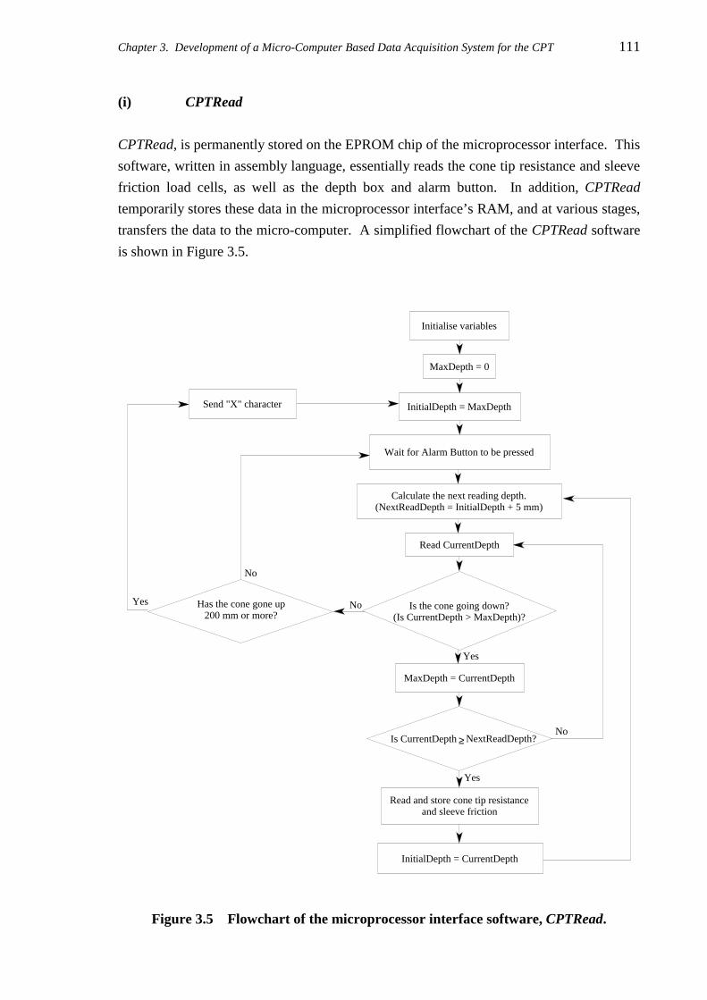
Chapter 3. Development of a Micro-Computer Based Data Acquisition System for the CPT 111
(i) CPTRead
CPTRead, is permanently stored on the EPROM chip of the microprocessor interface. This
software, written in assembly language, essentially reads the cone tip resistance and sleeve
friction load cells, as well as the depth box and alarm button. In addition, CPTRead
temporarily stores these data in the microprocessor interface’s RAM, and at various stages,
transfers the data to the micro-computer. A simplified flowchart of the CPTRead software
is shown in Figure 3.5.
Yes
No
Has the cone gone up200 mm or more?
NextReadDepth?Is CurrentDepth ≥
No
No
Yes
Yes
Send "X" character
InitialDepth = CurrentDepth
Read and store cone tip resistanceand sleeve friction
MaxDepth = CurrentDepth
Is the cone going down?(Is CurrentDepth > MaxDepth)?
Read CurrentDepth
Calculate the next reading depth.(NextReadDepth = InitialDepth + 5 mm)
Wait for Alarm Button to be pressed
InitialDepth = MaxDepth
MaxDepth = 0
Initialise variables
Figure 3.5 Flowchart of the microprocessor interface software, CPTRead.

112 Chapter 3. Development of a Micro-Computer Based Data Acquisition System for the CPT
In addition, CPTRead has an in built filtering algorithm for reducing the effects of
electrical noise. This aspect of CPTRead is detailed in §3.2.3.
(ii) CPTest
The program CPTest, written in Turbo Pascal® 10 Version 6.0, is the interface between the
operator of the CPT and the data acquisition system. Every 5 mm of travel of the cone
penetrometer, the microprocessor interface reads the cone and sleeve load cells and sends
depth, cone tip resistance and sleeve friction data to the RS232 port of the micro-computer.
An example of these data is shown below.
D2438
c0167
S0271
CPTest continually scans the RS232 port of the micro-computer for data being transferred
from the microprocessor interface. Data are read, one character at a time, and then
reassembled to form a series of three, string variables. Referring to the example above, the
first string would be “D2438”; the second “c0167”; and the third “S0271”. The first letter
of each string identifies the type of measurement. For example, a “D” character refers to a
depth measurement; a “c” character refers to a cone tip resistance measurement; and so on,
as described previously in §3.4.2.1.
In order to obtain the scaled values of depth, qc and fs , the digital values are multiplied by
conversion factors, as shown in Table 3.1, which were calculated using the relationships
shown in Table 3.2. Both of these tables are discussed in greater detail in §3.2.1.
Table 3.1 Data conversion factors.
First Character Measurement Conversion Factor Unit Range
D or M Depth 0.62832 mm 0 to 41,176 mm
c qc 0.014648 MPa 0 to 15 MPa
C qc × 5 0.0029296 MPa 0 to 3 MPa
S fs 0.48828 kPa 0 to 500 kPa
10 Turbo Pascal is a registered trademark of Borland International, P.O. Box 660001, Scotts Valley, CA, USA, 95066-
0001.
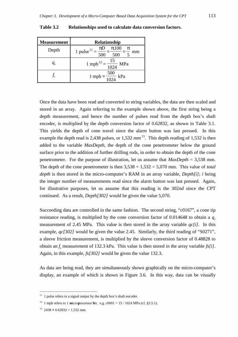
Chapter 3. Development of a Micro-Computer Based Data Acquisition System for the CPT 113
Table 3.2 Relationships used to calculate data conversion factors.
Measurement Relationship
Depth 1 pulse11 = π π πD
500
100
500 5= =
. mm
qc 1 mpb12 = 15
1024 MPa
fs 1500
1024 mpb kPa=
Once the data have been read and converted to string variables, the data are then scaled and
stored in an array. Again referring to the example shown above, the first string being a
depth measurement, and hence the number of pulses read from the depth box’s shaft
encoder, is multiplied by the depth conversion factor of 0.62832, as shown in Table 3.1.
This yields the depth of cone travel since the alarm button was last pressed. In this
example the depth read is 2,438 pulses, or 1,532 mm13. This depth reading of 1,532 is then
added to the variable MaxDepth, the depth of the cone penetrometer below the ground
surface prior to the addition of further drilling rods, in order to obtain the depth of the cone
penetrometer. For the purpose of illustration, let us assume that MaxDepth = 3,538 mm.
The depth of the cone penetrometer is then 3,538 + 1,532 = 5,070 mm. This value of total
depth is then stored in the micro-computer’s RAM in an array variable, Depth[i]; i being
the integer number of measurements read since the alarm button was last pressed. Again,
for illustrative purposes, let us assume that this reading is the 302nd since the CPT
continued. As a result, Depth[302] would be given the value 5,070.
Succeeding data are controlled in the same fashion. The second string, “c0167”, a cone tip
resistance reading, is multiplied by the cone conversion factor of 0.014648 to obtain a qc
measurement of 2.45 MPa. This value is then stored in the array variable qc[i]. In this
example, qc[302] would be given the value 2.45. Similarly, the third reading of “S0271”,
a sleeve friction measurement, is multiplied by the sleeve conversion factor of 0.48828 to
obtain an fs measurement of 132.3 kPa. This value is then stored in the array variable fs[i].
Again, in this example, fs[302] would be given the value 132.3.
As data are being read, they are simultaneously shown graphically on the micro-computer’s
display, an example of which is shown in Figure 3.6. In this way, data can be visually
11 1 pulse refers to a signal output by the depth box’s shaft encoder.
12 1 mpb refers to 1 microprocessor bit. e.g. c0001 = 15 / 1024 MPa (cf. §3.5.1).
13 2438 × 0.62832 = 1,532 mm.

114 Chapter 3. Development of a Micro-Computer Based Data Acquisition System for the CPT
Figure 3.6 An example of the CPTest screen.
monitored and interrogated in order to assess whether the test is being performed correctly
and whether it is giving sensible results. This is in accordance with ISOPT-1 (De Beer et
al., 1988) as described in §3.3.
Once the cone penetrometer has been raised more than 200 mm, the microprocessor
interface sends an “X” character to the micro-computer. Upon receiving this signal, which
implies that sampling has temporarily ceased due to the addition of further drilling rods,
CPTest again reads the depth box to determine the depth of the cone penetrometer and
assigns this depth to the variable MaxDepth. It is necessary for CPTest to read the depth
box at this maximum depth, since the depth of the cone penetrometer tip may not be at a
multiple of 5 mm. As a consequence, the depth of the penetrometer tip can be monitored
more accurately.
In addition, CPTest saves all data previously stored in the array variables, Depth[i], qc[i]
and fs[i], in the micro-computer’s RAM, to a file on a 3.5” floppy disk for later post-
processing. Data in the file are arranged in three columns: Depth of the cone tip below the
ground surface (mm); qc (MPa); and fs (kPa); and are saved in ASCII format - each column
being separated by a tab (ASCII #9) character.

Chapter 3. Development of a Micro-Computer Based Data Acquisition System for the CPT 115
3.1.2 Post-Processing
A number of computer programs have been developed to enable post-processing of the
CPT data recorded by CPTest. All programs were written in Turbo Pascal Version 6.0,
because of its excellent speed and graphical capabilities at the time of development. A
brief description of each of the programs is given below.
3.1.2.1 CPTView
The program CPTView was developed to allow the user to inspect, visually, the cone
penetration test data on the screen, both in the field and at a later date. Cone tip resistance,
sleeve friction and friction ratio are simultaneously plotted on the screen, an example of
which is shown in Figure 3.7. In addition, CPTView provides the following facilities:
• The entire CPT sounding can be plotted on a single screen;
• A range of depths can be plotted on a single screen, for example 2.5 metres to
5.0 metres;
• The entire recorded depth can be plotted and stepped in windows of user-specified
depth;
• The numerical values of qc , fs and FR , can be displayed for inspection.
3.1.2.2 CPTPlot
The program CPTPlot was developed to enable the user to prepare report quality plots and
tables of the CPT data stored on disk. Figure 3.8 shows an example of a graphical plot and
Figure 3.9 an example of the recorded CPT data printed in tabular format, each of which
has been produced by the CPTPlot program.
CPTPlot creates a PostScript14 file (filename.ps) which enables the plot, or table, to be
output to a laser printer which supports the PostScript language, such as the Apple Laser-
Writer.
In addition, CPTPlot shifts the sleeve friction data back by 75 mm. As detailed in §2.4.4,
this is necessary because the cone tip and the friction sleeve are physically separated by a
distance of 75 mm. As discussed previously, the microprocessor interface simultaneously
14 PostScript is a graphical language for laser printers developed by Adobe Systems, Inc.

116 Chapter 3. Development of a Micro-Computer Based Data Acquisition System for the CPT
Figure 3.7 An example of a screen plot produced by CPTView.
reads values of qc and fs at the depth of the cone penetrometer tip. As a result, the actual
depth corresponding to the fs measurements is 75 mm less than that indicated by the depth
box. Hence, friction ratio, FR , calculations, based on data that has not been corrected for
this shift, will yield misleading results (Schmertmann, 1978).
As discussed previously in §3.1.1.2(ii), measurements of qc and fs are read at depth
intervals of 5 mm. However, while the recorded depths are separated by 5 mm, they need
not be divisible by 5. This is due to the fact that MaxDepth, the maximum depth of the
cone penetrometer tip prior to the addition of further drilling rods, may not be at a depth
divisible by 5. For example, MaxDepth may be 797 mm and, when the CPT is continued,
the next depth at which readings are taken will be 797 + 5 mm, or 802 mm; a depth not
divisible by 5. When the fs measurements are shifted by 75 mm, there may not be a value
of qc corresponding to this depth, ie 652 mm. As a result, two columns of depths would
need to be provided: one for values of qc, and the other for the shifted values of fs .
So that only one column of depth measurements need be maintained, CPTPlot first

Chapter 3. Development of a Micro-Computer Based Data Acquisition System for the CPT 117
Figure 3.8 An example of a graphical plot produced by CPTPlot.

118 Chapter 3. Development of a Micro-Computer Based Data Acquisition System for the CPT
Figure 3.9 An example of a data table produced by CPTPlot.
Chapter 3. Development of a Micro-Computer Based Data Acquisition System for the CPT 119
rationalises the depths to values divisible by 5. For example, a depth of 797 mm would be
rationalised to 795 mm. The rationalisation algorithm obeys the following rules:
1. If the last digit is a 0, 1, or 2, then the last digit becomes a 0.
e.g. 200, 201 and 202 become 200 mm.
2. If the last digit is a 3, 4, 5, 6, or 7, then the last digit becomes a 5.
e.g. 203, 204, 205, 206, and 207 become 205 mm.
3. If the last digit is an 8, or 9, then the depth is increased by 2, or 1, respectively.
e.g. 208, and 209 become 210 mm.
The rationalisation process assumes that each measurement of qc and fs is constant within
its soil element of 5 mm in height. Such an assumption is appropriate for elements of soil
with such small dimensions. Once rationalisation of depths has been performed, the sleeve
friction values can then be easily shifted back by 75 mm.
Occasionally, the distance between two successive depth measurements is 6 mm instead of
5 mm. The reason for this is explained in §3.2. As a result, rationalisation causes some
depths to have no associated qc or fs measurements. For example, two successive depths
may be 207 mm and 213 mm, that is, separated by 6 mm. Upon rationalisation, the
207 mm depth becomes 205 mm; and the 213 mm depth becomes 215 mm. Hence, the
210 mm depth has no associated qc or fs measurements. When this occurs, CPTPlot,
assigns this missing depth of 210 mm with values of qc and fs equal to −99.99, implying
that there are missing data associated with this depth. When plotting takes place, CPTPlot
(and CPTView) ignores these missing data and draws a straight line from the next depth
above and below this missing depth.
Rationalised plots of data spaced at 5 mm intervals are indistinguishable from
unrationalised plots. Figure 3.8 shows an example of a plot performed on rationalised data,
and Figure 3.10 shows the same data but plotted without depth rationalisation. As can be
seen clearly from these figures, these missing data have negligible effect on the plots
obtained by CPTPlot. Note the effect of rationalisation and sleeve friction shift on the plot
of friction ratio versus depth. Omission of the shift can greatly affect the calculation of FR
yielding misleading results, as mentioned previously.
In addition, it will be seen later, in Chapter 5, that the rationalisation process simplifies the
calculation of the semivariogram, autocorrelation and partial autocorrelation functions, as
well as reducing their calculation times.
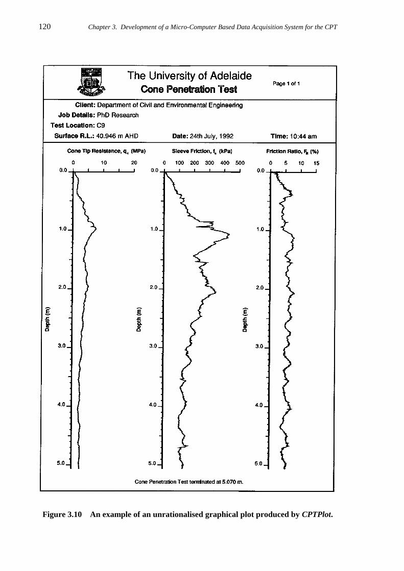
120 Chapter 3. Development of a Micro-Computer Based Data Acquisition System for the CPT
Figure 3.10 An example of an unrationalised graphical plot produced by CPTPlot.
Chapter 3. Development of a Micro-Computer Based Data Acquisition System for the CPT 121
In addition to those discussed previously, CPTPlot provides the following features:
• One, two or five metres of data, or the entire data set, can be plotted on a single page;
• Either of the following formats can be plotted:
• cone tip resistance, sleeve friction and friction ratio, or
• cone tip resistance, friction ratio and undrained shear strength.
3.1.2.3 CPTPrint
CPTPrint is a utility program which enables files created by CPTPlot to be printed by the
Apple LaserWriter, or other PostScript printing device. So that the University of Adelaide
crest can be printed at the top left hand corner of each plot, CPTPrint either copies or
concatenates (depending on whether the user has a stand-alone PC15 connected to the
printer, or a networked PC) the plot file with the university crest file (crest.ps). In this
way, plot files can be stored more efficiently without duplicating the crest in each plot file.
A typical 5 metre plot file is approximately 80 kb in size, whereas crest.ps is about
17 kb in size.
3.1.3 Description of Overall Data Acquisition System
The University of Adelaide data acquisition system was developed to enable closely-spaced
CPT data to be measured and stored reliably, efficiently and accurately. As discussed
previously, the data acquisition system can be divided into hardware and software. The
hardware of the system consists of: the electric cone penetrometer; depth box; alarm
button; microprocessor interface; and the micro-computer. The software of the data
acquisition system consists of: CPTRead; CPTest; CPTView; CPTPlot; and CPTPrint. A
summary of the University of Adelaide data acquisition system for the cone penetration test
is shown in flowchart form in Figure 3.11.
Each of the elements of the data acquisition system is powered by a 12V DC16 source,
which is normally supplied by the lead-acid battery on board the drilling rig. The battery
provides a stable power source which readily accommodates the requirements of the
individual components of the system.
15 Personal Computer
16 Direct Current.

122 Chapter 3. Development of a Micro-Computer Based Data Acquisition System for the CPT
Figure 3.11 Flowchart of the University of Adelaide CPT data acquisition system.

Chapter 3. Development of a Micro-Computer Based Data Acquisition System for the CPT 123
3.2 CALIBRATION AND ACCURACY OF EQUIPMENT
Micro-computer based data acquisition systems, by themselves, do not increase the
accuracy of the recorded data. The accuracy is derived from the design and quality of the
individual elements and electrical components, as well as the quality and resolution of the
microprocessor interface and associated software. This section details the procedures and
the results of calibration tests undertaken to quantify the resolution, accuracy and errors
associated with the University of Adelaide data acquisition system for the CPT, and
compares these to the criteria specified in §3.3.
3.2.1 Resolution of Measured Data
The accuracy of the CPT data is governed by the resolution of the microprocessor interface
and the depth box. Since the acquisition system stores and transfers data digitally, the
recorded values of depth, cone tip resistance and sleeve friction, have a finite resolution.
The resolution of depth measurements is dictated by the specifications of the shaft encoder,
that is, 500 pulses per revolution of the encoder. Since the depth box drum has a diameter
of 100 mm, the resolution of depth measurements is π 5, or 0.628 mm, as indicated
previously in Tables 3.1 and 3.2.
The resolution of qc and fs measurements is governed by the number of bits that the A/D
converter of the MPU can accommodate. The University of Adelaide microprocessor
interface contains an MPU with a 10 bit A/D converter, as shown in Figure 3.5. Hence,
since the MPU can accommodate 210, or 1,024 values, and the range of qc and fs
measurements is 15 MPa and 500 kPa respectively, the resolution of cone tip resistance
measurements is 15 1024, or 14.65 kPa, and the resolution of sleeve friction measurements
is 500 1024 , or 0.488 kPa, as shown in Tables 3.1 and 3.2.
3.2.2 Calibration Tests to Quantify Measurement Errors
This section discusses the results of calibration tests undertaken to quantify errors in the
measurement of qc, fs and depth, and examines how well each of these compares with the
criteria specified in §3.3.

124 Chapter 3. Development of a Micro-Computer Based Data Acquisition System for the CPT
3.2.2.1 Depth Box and Depth Measurements
The depth box, and the resulting measurement of depth, was calibrated by comparing the
results output by the microprocessor interface to those given by a 500 mm long vernier and
an 8 metre long steel tape. The results of the calibration are shown in Figure 3.12.
0
0
0
0
0
0
0
0
0
0
0
0
0
0
0
00
0000000000000
2000
4000
6000
8000
10000
0 2000 4000 6000 8000 10000
0 Measured Values
Equality
Actual Depth (mm)
Figure 3.12 Depth box calibration curve.
The results of the calibration indicate that the accuracy of the depth box is 0.8%, that is, an
error of 160 mm in 20 metres. While this error is approximately 3 times greater than that
specified by de Ruiter (1981), it still represents a relatively high degree of accuracy.
This error can, in part, be attributed to the diameter of the metal drum of the depth box. As
discussed in §3.1.1.2(ii), the microprocessor interface reads both the cone tip load cell and
the sleeve friction load cell at depth intervals of 5 mm. However, every 38th measurement
the distance between two successive depth readings is 6 mm instead of 5 mm. This is
because of rounding of the depth conversion factor, indicated in Table 3.1. The
microprocessor interface reads the qc and fs load cells every 8 pulses of the shaft encoder.
However, a penetration depth of 5 mm actually corresponds to 7.9577 pulses, not eight.
Every 38 readings, or 190 mm, this error accumulates to add 1 mm to the depth, that is, an
inaccuracy of 0.53%.
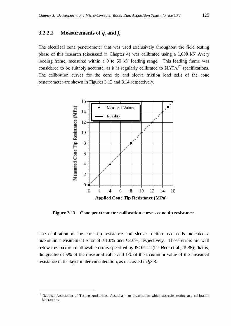
Chapter 3. Development of a Micro-Computer Based Data Acquisition System for the CPT 125
3.2.2.2 Measurements of qc and fs
The electrical cone penetrometer that was used exclusively throughout the field testing
phase of this research (discussed in Chapter 4) was calibrated using a 1,000 kN Avery
loading frame, measured within a 0 to 50 kN loading range. This loading frame was
considered to be suitably accurate, as it is regularly calibrated to NATA17 specifications.
The calibration curves for the cone tip and sleeve friction load cells of the cone
penetrometer are shown in Figures 3.13 and 3.14 respectively.
0
0
0
0
0
0
0
0
00
2
4
6
8
10
12
14
16
0 2 4 6 8 10 12 14 16
0 Measured Values
Equality
Applied Cone Tip Resistance (MPa)
Figure 3.13 Cone penetrometer calibration curve - cone tip resistance.
The calibration of the cone tip resistance and sleeve friction load cells indicated a
maximum measurement error of ±1.0% and ±2.6%, respectively. These errors are well
below the maximum allowable errors specified by ISOPT-1 (De Beer et al., 1988); that is,
the greater of 5% of the measured value and 1% of the maximum value of the measured
resistance in the layer under consideration, as discussed in §3.3.
17 National Association of Testing Authorities, Australia - an organisation which accredits testing and calibration
laboratories.

126 Chapter 3. Development of a Micro-Computer Based Data Acquisition System for the CPT
0
0
0
0
0
0
0
00
100
200
300
400
500
0 100 200 300 400 500
0 Measured Values
Equality
Applied Sleeve Friction (kPa)
Figure 3.14 Cone penetrometer calibration curve - sleeve friction.
3.2.2.3 Microprocessor Interface Sampling Rate
The microprocessor interface has a sample interval of approximately 0.1 second. As
mentioned in §3.3, Jamiolkowski et al. (1985) recommended that CPT data be sampled
within the range of 0.1 to 1 second; whereas Lunne et al. (1986) suggested a 1 second
sample interval is generally adequate. Depth measurements, or pulses from the depth box’s
shaft encoder, are interrupt driven. That is, the MPU immediately processes these
measurements as soon as an interrupt signal is received. As a result, depth measurements
can be recorded at a maximum sampling rate of 75 µs, the sample and conversion rate of
the microprocessor. At the standard penetration rate of 20 mm/s, the shaft encoder
transmits approximately 32 pulses per second, which is equivalent to one pulse every
31 ms. As a result, a sample rate of 75 µs, which is approximately 2,500 times greater than
the rate of pulse transmission, is more than adequate to measure depth, qc and fs .
3.2.3 Random Measurement Errors
Random measurement errors, such as electrical noise, although generally small, are always
present in this type of system in one form or another. In order to minimise random
measurement errors, a filtering algorithm was built into the program CPTRead. This
algorithm effectively uses a four level stack. Measured data are placed at the bottom of the
Chapter 3. Development of a Micro-Computer Based Data Acquisition System for the CPT 127
stack and each previous measurement is rolled up to the next level on the stack, the
uppermost value being rolled off the stack. An average of the four values on the stack is
calculated each time new data are measured. In this way a rolling average of the data is
recorded. Davison and Hills (1983) suggested a similar method for reducing the
fluctuation in readings due to electrical noise, described as 12% trimmed means. This
method stores 24 readings which are ranked, the top and bottom four are discarded, and the
result stored in memory being the average of the remaining 16. Calibration tests, detailed
in the preceding section, indicated that the rolling average method is an effective and
adequate means of minimising the effect of electrical and random noise, and there was no
need to adopt Davison and Hills’ 12% trimmed means technique.
3.3 FIELD PERFORMANCE
Tests to assess the field performance of the University of Adelaide data acquisition system
showed that it is relatively robust and performs well in a variety of weather conditions.
The tests, however, highlighted two problems with the equipment and associated software:
falling off; and noise spikes. These are shown in Figure 3.15 and are treated in-turn, below.
3.3.1 Falling Off
Assessment of the data measured during preliminary cone penetration tests indicated that at
every addition of a drill rod the measured values of qc and fs dropped to zero, or a value
well below that recorded immediately above it. This phenomenon, known as falling off, as
shown in Figure 3.15, is indicated only at the addition of further drill rods and at no other
point in the CPT sounding. The cause of falling off is likely to be due to a number of
factors, which include:
• Soil rebound - Since much of the soil surrounding the electric cone penetrometer
remains in an elastic condition, as shown in Figure 2.9, when load is removed from the
drill rod stem to enable further rods to be added, the surrounding soil rebounds thereby
lifting the penetrometer slightly and reducing the measurements of qc and fs to values
approaching zero.
• Response of electrical components - The time taken for the cone tip resistance and
sleeve friction load cells to respond to large changes may be such that the response
recorded is principally that of the equipment and not the soil.
The effect of falling off has been removed by modifications to the control program CPTest.

128 Chapter 3. Development of a Micro-Computer Based Data Acquisition System for the CPT
Figure 3.15 An example of qc and fs falling-off at rod changes and noise spikes.

Chapter 3. Development of a Micro-Computer Based Data Acquisition System for the CPT 129
Measurements of qc and fs are recorded at intervals of 5 mm from the initiation and
continuation of the CPT. However, as discussed previously, when the data are saved to the
data file on the floppy disk, CPTest does not save the first 2 readings. This removes the
falling off effect in qc and fs measurements, but adds to the number of missing depths in the
data file, as discussed in §3.1.1.2(ii).
3.3.2 Noise Spikes
An uncertainty associated with the measurement of qc and fs , discovered during the
development of the data acquisition system, was the random presence of noise spikes.
These were identified as sudden increases in qc and fs values that were not associated with
any geotechnical phenomena. Figure 3.15 shows examples of noise spikes obtained during
cone penetration testing. These spikes were found to be related to earthing within the CPT
cable, and rectified by connecting the shielding that surrounds the cable and individual
wires, to ground.
3.3.3 Limitations of Data Acquisition System
A computer based data acquisition system has two drawbacks. Firstly, minor undetected
defects, such as gradual breakdown of the electrical instruments, amplifiers and electrical
components, give rise to data inaccuracy and an increased measurement error (defined as
the difference between the actual parameter and that measured) with time. This error can
be minimised, however, by regular calibration. ISOPT-1 (De Beer et al., 1988)
recommends that calibration be carried out at least every three months.
Secondly, total failure of the system can occur due to failures of the micro-computer, or
microprocessor interface, which usually occur due to external power supply failure. The
University of Adelaide system is less likely to suffer from power supply failure since the
external power source is derived from the vehicle’s 12V battery - the power required to
drive the various electrical elements of the data acquisition system being insignificant in
comparison to that stored in the battery itself.
3.4 SUMMARY
This chapter has examined the development of a micro-computer based data acquisition
system for the CPT. It has been shown that the system satisfies each of the criteria

130 Chapter 3. Development of a Micro-Computer Based Data Acquisition System for the CPT
specified in §3.3. As a result, the data acquisition system is a robust and reliable means of
accurately measuring, recording and storing closely-spaced CPT data.
The data acquisition system will be used in a field study to measure the small-scale spatial
variability of the Keswick and Hindmarsh Clays. This field study is detailed in the next
chapter.

131
Chapter Four
Experimental Programme
4.1 INTRODUCTION
As mentioned previously, in order to quantify small-scale variation (that is, within the
range of millimetres to metres) it is necessary to obtain data at closely spaced intervals -
both vertically and horizontally. This chapter details the results of a field study undertaken
to quantify the small-scale variation of the undrained shear strength, su , of the Keswick and
Hindmarsh Clays. Chapter 6, on the other hand, will discuss the compilation of a data base
which will be used to quantify the large-scale variability of these clays.
4.2 LOCATION OF SITE FOR FIELD STUDY
In selecting the site for the field investigation, it was decided that it should meet a number
of criteria. That is, the site should:
• be located within the Adelaide city area - so that the field study data can be incorporated
with the large-scale database (discussed in Chapter 6);
• have minimum dimensions of 50 × 50 metres - in order to enable the number of required
tests to be carried out;
• be relatively free of trees and vegetation - Trees and vegetation draw water from the
upper region of the subsurface profile resulting in moisture changes with depth. These
moisture variations influence the shear strength of the soil which, in turn, can distort
spatial variability analyses. In addition, the locations of the trees will influence the
positions of the individual tests and unnecessarily complicate the testing programme;

132 Chapter 4. Experimental Programme
• have the Keswick and Hindmarsh Clays relatively close to the ground surface -in order
to optimise the testing programme by obviating the need for unnecessary drilling and
penetration;
• be relatively flat and free of fill, previous construction and services - thereby reducing
the number of aspects likely to hinder the testing programme and uncertainties
associated with the measurements;
• have clear access to the site - enabling the drilling rig and associated equipment to enter
the site and successfully carry out the testing programme.
A suitable site, which satisfied the criteria listed above, was located in the South Parklands
of the City of Adelaide. The location of the field study site is shown in Figure 4.1.
4.3 FIELD TESTING - SOUTH PARKLANDS SITE
As discussed in Chapters 1 and 2, the cone penetration test (CPT) was used as the basic
field testing procedure to quantify the small-scale variability of the Keswick and
Hindmarsh Clays because:
• In situ testing has a number of advantages over laboratory testing;
• Large amounts of data can be acquired efficiently and economically;
• The CPT has the lowest measurement error of any in situ test method in current use;
• CPT equipment and technicians proficient in its operation were available.
4.3.1 Layout of Field Testing
In order to determine the small-scale variability of the Keswick and Hindmarsh Clays in
the vertical direction, as well as in a number of horizontal directions, a grid layout of cone
penetration tests was chosen, as shown in Figure 4.2.
The layout consisted of 100 CPTs at a grid spacing of 5 metres in both directions, and 101
CPTs set out in a cross arrangement at lateral spacings of 1 metre. For ease of referencing,
an alpha-numeric grid-numbering system was adopted, as shown in Figure 4.2. The
referencing system used for the CPTs in the cross arrangement is shown in Figure 4.3. It
was proposed that each cone penetration sounding would be performed to a depth of
5 metres below ground. Thus, for each sounding, a total of 1,000 measurements of cone tip

Chapter 4. Experimental Programme 133
Figure 4.1 Location of field study site.

134 Chapter 4. Experimental Programme
5 m
50 m
50 m
5 m
1 m
1 m
0 1 2 3 4 5 6 7 8 9 10A
B
C
D
E
F
G
H
I
J
K
CPT location
LegendGridNorth
Figure 4.2 Initial layout of field testing.
resistance, qc , and sleeve friction, fs , would be recorded, due to the spacing of
measurements being 5 mm, as detailed in Chapter 3. The orientation of the CPTs, as
shown in Figure 4.1, was chosen to avoid large trees, overhead electrical cables and a
concrete cricket pitch.
It is common practice, when investigating the spatial variability of soils and rock, to use a
sampling pattern which is regular and either in the form of a square grid, or along a straight
line. In particular, in the field of geostatistics, it is common place to use regular square grid
sampling (Brooker, 1975; Journel and Huijbregts, 1978; Clark, 1979; Rendu, 1981; Azzouz
and Bacconnet, 1991; Brooker, 1991). Journel and Huijbregts (1978) recommended that,
initially, sampling should be carried out on a large, and more or less, regular grid which is

Chapter 4. Experimental Programme 135
0 1 2 3 4 5 6 7 8 9 10A
B
C
D
E
F
G
H
I
J
K
A5
B5
C5
B51B52B53B54
A51A52A53A54
C51
F0
F01
F02
F03
F04
F1 F2
F11
F12
F13
F14
F21
F5
F501
F502
F503
F504
F6
F61
Figure 4.3 Referencing system used for the one metre, laterally spaced CPTs.
then followed by in-fill drilling, that is, sampling on a progressively smaller grid.
Furthermore, it is possible to show, using geostatistics, that samples located on a regular, or
near regular grid, provide more information than randomly located samples (Matheron,
1963; Rendu, 1981).
In the application of random field theory to the spatial variability of geotechnical materials,
it is common practice to use either: samples taken along straight lines at regular, or
irregular, intervals (Lumb, 1974, 1975; Anderson et al., 1984; Bergado et al., 1992); or
samples obtained from regular, or near regular, square grids (Tang, 1979; Smith, 1981;
Fardis and Veneziano, 1981). As shown in Figure 4.2, the proposed testing layout
conforms with sampling regimes generally accepted in both the fields of geostatistics and
random field theory.
4.3.2 Equipment and Methods
So that the results of the field testing would enable an accurate assessment of the spatial
variability of undrained shear strength to be made, it was essential that testing be carried

136 Chapter 4. Experimental Programme
out over as short a period of time as possible. This was to ensure that moisture variations
within the subsurface profile, caused by seasonal effects, would be kept to a minimum. In
order to achieve this, the use of a large-capacity drilling rig was necessary. The
Department of Road Transport of South Australia owns and operates two such rigs: an
Edson; and a Proline. These are shown in Figures 4.4 and 4.5, respectively. Subsequent to
a request by the author, the Department generously agreed to provide a rig and an operator
for the duration of this study. With the use of these rigs, it was anticipated that the testing
programme would be completed within a period of one month.
Figure 4.4 Edson drilling rig.
In addition, the Department of Civil and Environmental Engineering at the University of
Adelaide owns and operates a light-weight, Toyota, four-wheel-drive, drilling rig, as shown
in Figure 4.6. It weighs approximately 2 tonnes and has a driving capacity of around
4 tonnes when fitted with two ground anchors.
The hydraulic feed rate, or the rate of cone penetration, of both the Edson and Proline
drilling rigs is controlled manually by the operator. In order to minimise the uncertainties
associated with the cone penetration tests, one driller, Mr. Ian Forrester, exclusively
operated the Edson and Proline drilling rigs throughout the testing programme. On the
other hand, the Toyota drilling rig is fitted with an hydraulic pressure regulator which

Chapter 4. Experimental Programme 137
Figure 4.5 Proline drilling rig.
Figure 4.6 Toyota 4WD drilling rig.

138 Chapter 4. Experimental Programme
ensures that the rate of penetration is maintained at 20 mm/s regardless of the resistance
offered by the soil. As a consequence, the cone penetration rate is effectively operator-
independent. However, throughout the testing programme, the Toyota drilling rig was
exclusively operated by Mr. Tad Sawosko.
The hydraulic feed rate of the Edson and Proline rigs was monitored throughout the field
study and the CPTs were maintained at a penetration rate of between 10 and 20 mm/s, as
specified by AS 1289.F5.1 (Standards Association of Australia, 1977). Field testing
occurred over three periods: from July to August 1992; in September 1992; and from
February to March 1993. Table 4.1 details the schedule of the cone penetration tests.
The CPTs were carried out in accordance with AS 1289.F5.1 (Standards Association of
Australia, 1977) and ISOPT-1 (De Beer et al., 1988) using a standard, 35.7 mm diameter,
electrical friction-cone penetrometer, as detailed in §2.4.2, §2.4.3 and §3.4.1.1. Typical
results obtained from the cone penetration tests are included in Appendix A.
The field testing programme extended for a total of approximately 7 months, far greater
than that initially expected. This was due mainly to the fact that the drilling rigs were often
needed for other commitments and, as a consequence, the rigs were often unavailable for
the study. In addition, a period of heavy winter rain was experienced in late August and
September 1992, causing disruption to the testing programme. Tests performed on the
29th September 1992 indicated that the recent rainfall had significantly affected the
subsurface moisture regime and, hence, subsequent testing could not be used in the same
data set. Thus, it was decided to abort the original testing programme and layout. From
the beginning of testing to the 29th September 1992, 177 CPTs were successfully carried
out. Five (those that were performed on the 29th September) were deemed to be
unacceptable because of the recent winter rains and, hence, were discarded from the data
set, leaving 172 CPTs that could be used for the assessment of the small-scale variability of
the Keswick and Hindmarsh Clays. It will be shown in §4.3.4 that during the period of the
3rd July 1992 to the 14th August 1992, when these 172 CPTs were measured, the climatic
conditions were relatively constant and, hence, the subsurface moisture regime was also
relatively stable.
Preliminary analyses of the spatial variability of the test results obtained to that date
showed that, in order to quantify the lateral variability of the Keswick Clay, samples should
be taken at intervals of less than one metre (Jaksa et al., 1993). As a consequence, it was
decided to amend the testing layout to include 50 CPTs at lateral spacings of 0.5 metres.
These tests, CD1 to CD50, were performed between the 16th - 18th February 1993. The
layout of all field tests that were carried out at the South Parklands site are summarised in
Figure 4.7.

Chapter 4. Experimental Programme 139
Table 4.1 Cone penetration testing programme.(CPT reference system is shown in Figures 4.3 and 4.7).
Date Drilling Rig No. of CPTs CPTs3rd July 1992 Proline 14 K5, J54, J53, J52, J51, J5, I54, I53, I52, I51,
I5, H54, H53, H527th July 1992 Edson 15 F5, F51, F52, F53, F54, G5, G51, G52, G53,
G54, H5, H51, A5, A51, A529th July 1992 Edson 20 A53, A54, B5, B51, B52, B53, B54, C5, C51,
C52, C53, C54, D5, D51, D52, D53, D54,E5, E51, E52
10th July 1992 Proline 5 E53, E54, F44, F43, F42
14th July 1992 Proline 19 F10, F94, F93, F92, F91, F9, F84, F83, F82,F81, F8, F74, F73, F72, F71, F7, F64, F63,
F6215th July 1992 Proline 10 F61, F6, F504, F503, F502, F501, F33, F32,
F31, F2416th July 1992 Proline 16 F22, F21, F2, F14, F13, F12, F11, F1, A10,
B10, C10, D10, G10, H10, I10, J1017th July 1992 Proline 13 E10, K10, K9, K8, K7, K6, K4, K3, K2, A0,
A1, A4, A624th July 1992 Proline 15 A8, B9, C9, D9, E9, G9, H9, I9, J9, B8, C8,
D8, E8, G8, H829th July 1992 Proline 14 J8, B7, C7, D7, E7, G7, H7, I7, J7, B6, C6,
D6, E6, G631st July 1992 Proline 10 H6, I6, J6, B4, C4, D4, E4, G4, I4, J4
14th August 1992 Edson 21 B0, C0, D0, E0, F0, G0, H0, I0, J0, B1, C1,D1, E1, G1, H1, I1, J1, K1, K0, A2, B2
29th September 1992 Edson 5 A3, B3, C3, D3, E3
16th February 1993 Edson 18 CD50, CD49, CD48, CD47, CD46, CD45,CD44, CD43, CD42, CD41, CD40, CD39,CD38, CD37, CD36, CD35, CD34, CD33
17th February 1993 Edson 14 CD32, CD30, CD29, CD28, CD27, CD26,CD25, CD24, CD23, CD22, CD21, CD20,
CD19, CD1718th February 1993 Edson 18 CD31, CD18, CD16, CD15, CD14, CD13,
CD12, CD11, CD10, CD9, CD8, CD7, CD6,CD5, CD4, CD3, CD2, CD1
26th February 1993 Edson 3 A10A. A10B, A10C
4th March 1993 Toyota 3 F5A, F5B, F5C
4.3.3 Sampling and Logging
In order to correlate cone tip resistances, measured in the field study, with undrained shear
strengths, obtained from the data base, KESWICK, to be discussed in Chapter 6, it was
necessary to obtain samples for unconsolidated undrained triaxial testing. Such tests would
enable the determination of the cone factor, Nk , as detailed in §2.4.5. Two boreholes, A10
and F5, were drilled for this purpose, the locations of which are shown in Figure 4.7.

140 Chapter 4. Experimental Programme
5 m
50 m
5 m
1 m
1 m
0 1 2 3 4 5 6 7 8 9 10A
B
C
D
E
F
G
H
I
J
K
2.5 m
CD1
CD50
0.5 m
50 m
Legend
Continuous core sample
3.3
2.4
1.6
2.3
1.1
2.2
2.0
2.3
1.0 Depth to top of Keswick Clay
Unsuccessful soundings
Successful soundings
GridNorth
3.4
Triaxial samples
Figure 4.7 Amended testing layout.
The first of these boreholes, A10, was drilled on 26th February 1993 using the Department
of Road Transport’s Edson rig. The second borehole, F5, was drilled on 4th March 1993
using the University’s Toyota 4WD drilling rig. Each sample consisted of a 70 mm
diameter thin-walled tube which was sealed against moisture loss using screw-fit plastic
seals. A total of 12 undisturbed samples of Keswick Clay were subsequently tested in the
laboratory, the results and discussion of which are detailed in §4.5.

Chapter 4. Experimental Programme 141
Eight boreholes were drilled on 15th August 1992, to a depth of 5 metres below ground, to
provide continuous cores for the purpose of visual inspection and logging of the subsurface
profile. These were achieved using the dynamic-push technique; that is, where a series of
40 mm diameter tubes, 1.0 metres in length, are dynamically driven into the soil, thereby
providing a continuous, although disturbed, core of the subsurface material. The locations
of these boreholes are also shown in Figure 4.7. A summary of the borehole logs is shown
in Table 4.2 and Figure 4.8, and the complete borehole logs are included in Appendix B.
Table 4.2 Summary of borehole logs.
Borehole Depth to top ofcalcareous layer (m)
Depth to top ofKeswick Clay (m)
A0 0.4 2.3A10 1.1 3.4C2 0.7 2.3C8 0.2 1.1F5 0.3 1.6I2 0.5 2.4I8 1.0 2.2K0 0.5 3.3K10 0.3 2.0
4.3.4 Reduction of Errors During Field Testing
In order to measure the spatial variability of any geotechnical materials it is essential to
eliminate variabilities associated with other effects, such as equipment, operator and
procedural variabilities, as well as temporal climatic changes. As discussed previously, so
that equipment and operator errors would be minimised, a single cone penetrometer, data
acquisition system and operator were used throughout the field testing programme. In
addition, the procedure adopted for each of the CPTs conformed with the standards
specified by AS 1289.F5.1 (Standards Association of Australia, 1977) and ISOPT-1 (De
Beer et al., 1988).
So that the temperature of the cone penetrometer was relatively constant throughout
testing, the following procedure was adopted:
1. Prior to each group of CPTs (at the commencement of each day, or after a refreshment
break), the cone penetrometer was inserted about 300 mm into the ground for
approximately 5 to 10 minutes. This was performed in accordance with AS 1289.F5.1,
so that the cone was able to equilibrate with the subsurface temperature.

142 Chapter 4. Experimental Programme
Figure 4.8 Graphical representation of borehole logs. Contours to surface of:
(a) Calcareous Mantle; (b) Limy Surficial Layer; (c) Keswick Clay, to AHD;
and (d) 3D representation.
2. Following each CPT, while the drilling rig was being moved to the location of the next
CPT, the cone penetrometer was covered by an insulating blanket to shield it from direct
sunlight and to maintain its temperature with that of the subsurface.
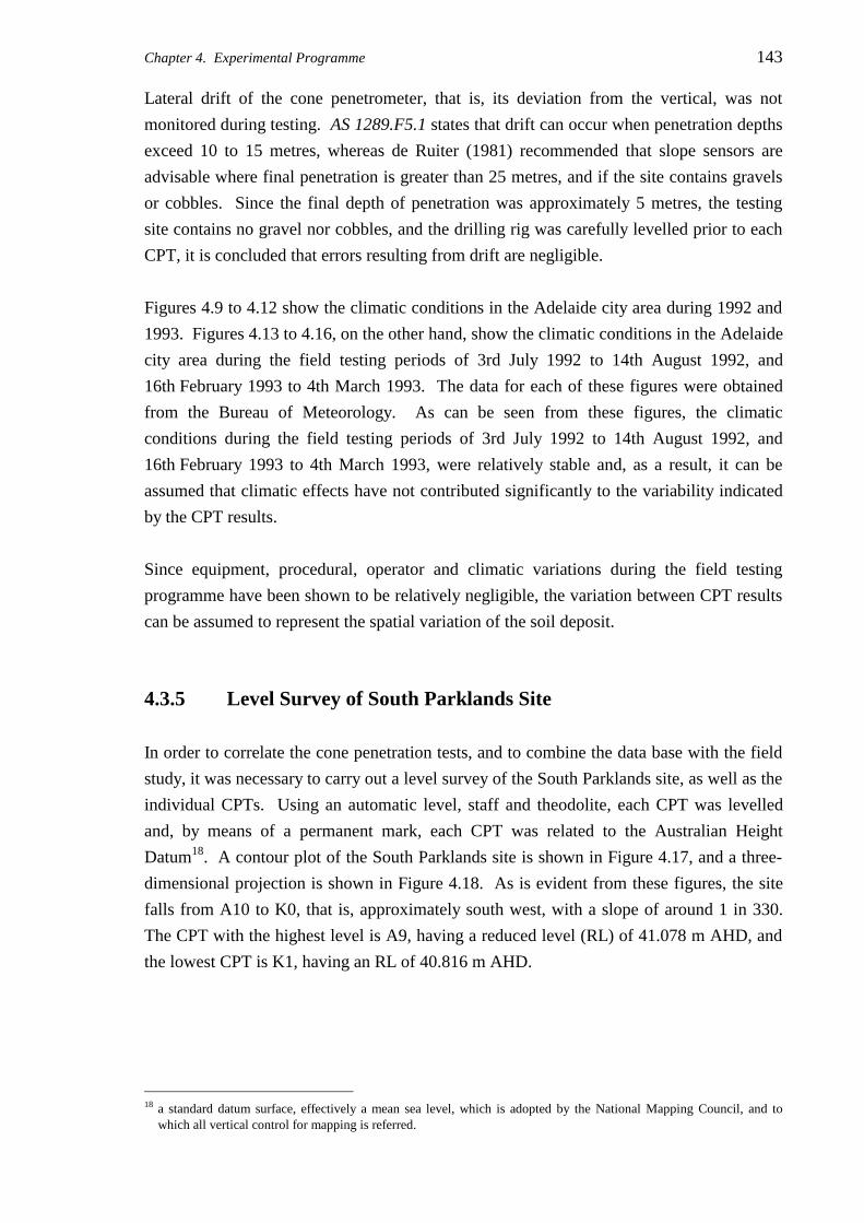
Chapter 4. Experimental Programme 143
Lateral drift of the cone penetrometer, that is, its deviation from the vertical, was not
monitored during testing. AS 1289.F5.1 states that drift can occur when penetration depths
exceed 10 to 15 metres, whereas de Ruiter (1981) recommended that slope sensors are
advisable where final penetration is greater than 25 metres, and if the site contains gravels
or cobbles. Since the final depth of penetration was approximately 5 metres, the testing
site contains no gravel nor cobbles, and the drilling rig was carefully levelled prior to each
CPT, it is concluded that errors resulting from drift are negligible.
Figures 4.9 to 4.12 show the climatic conditions in the Adelaide city area during 1992 and
1993. Figures 4.13 to 4.16, on the other hand, show the climatic conditions in the Adelaide
city area during the field testing periods of 3rd July 1992 to 14th August 1992, and
16th February 1993 to 4th March 1993. The data for each of these figures were obtained
from the Bureau of Meteorology. As can be seen from these figures, the climatic
conditions during the field testing periods of 3rd July 1992 to 14th August 1992, and
16th February 1993 to 4th March 1993, were relatively stable and, as a result, it can be
assumed that climatic effects have not contributed significantly to the variability indicated
by the CPT results.
Since equipment, procedural, operator and climatic variations during the field testing
programme have been shown to be relatively negligible, the variation between CPT results
can be assumed to represent the spatial variation of the soil deposit.
4.3.5 Level Survey of South Parklands Site
In order to correlate the cone penetration tests, and to combine the data base with the field
study, it was necessary to carry out a level survey of the South Parklands site, as well as the
individual CPTs. Using an automatic level, staff and theodolite, each CPT was levelled
and, by means of a permanent mark, each CPT was related to the Australian Height
Datum18. A contour plot of the South Parklands site is shown in Figure 4.17, and a three-
dimensional projection is shown in Figure 4.18. As is evident from these figures, the site
falls from A10 to K0, that is, approximately south west, with a slope of around 1 in 330.
The CPT with the highest level is A9, having a reduced level (RL) of 41.078 m AHD, and
the lowest CPT is K1, having an RL of 40.816 m AHD.
18 a standard datum surface, effectively a mean sea level, which is adopted by the National Mapping Council, and to
which all vertical control for mapping is referred.
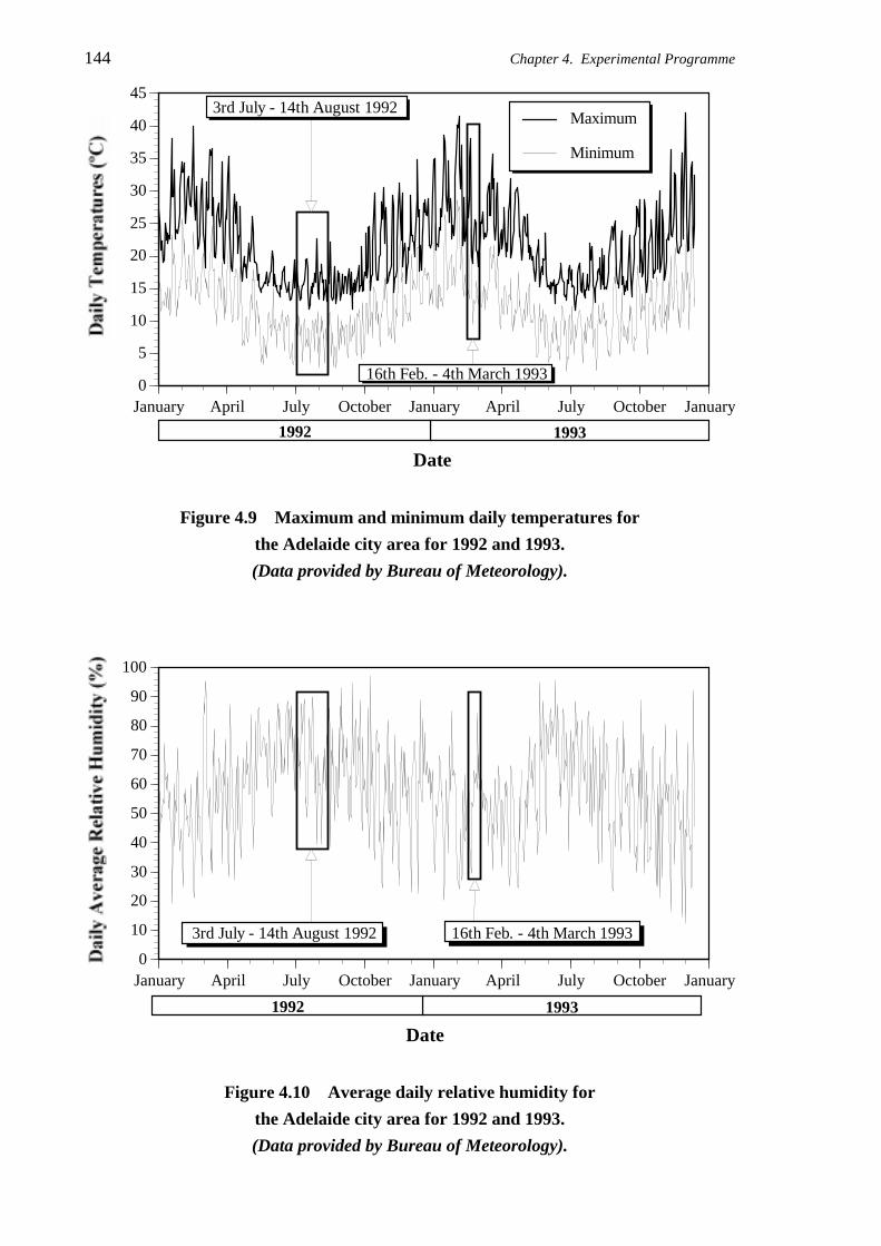
144 Chapter 4. Experimental Programme
0
5
10
15
20
25
30
35
40
45
January April July October January April July October January
Maximum
Minimum
1992 1993
Date
3rd July - 14th August 1992
16th Feb. - 4th March 1993
Figure 4.9 Maximum and minimum daily temperatures for
the Adelaide city area for 1992 and 1993.
(Data provided by Bureau of Meteorology).
0
10
20
30
40
50
60
70
80
90
100
January April July October January April July October January
1992 1993
Date
3rd July - 14th August 1992 16th Feb. - 4th March 1993
Figure 4.10 Average daily relative humidity for
the Adelaide city area for 1992 and 1993.
(Data provided by Bureau of Meteorology).

Chapter 4. Experimental Programme 145
0
5
10
15
20
25
30
35
40
45
January April July October January April July October January
1992 1993
Date
3rd July - 14thAugust 1992
16th Feb. - 4th March 1993
Figure 4.11 Daily rainfall for the Adelaide city area for 1992 and 1993.
(Data provided by Bureau of Meteorology).
0
2
4
6
8
10
12
14
January April July October January April July October January
1992 1993
Date
3rd July - 14th August 1992 16th Feb. - 4th March 1993
Figure 4.12 Daily evaporation for the Adelaide city area for 1992 and 1993.
(Data provided by Bureau of Meteorology).
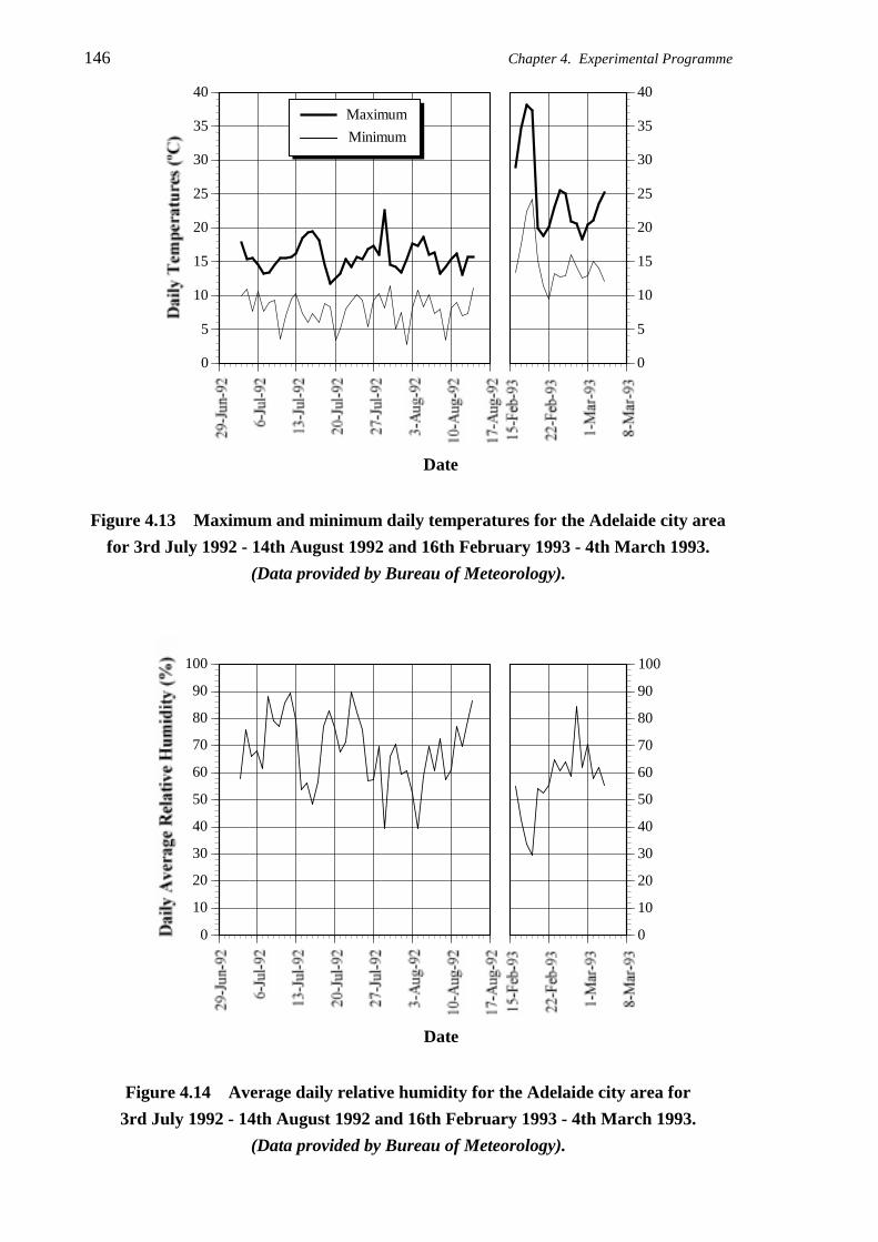
146 Chapter 4. Experimental Programme
0
5
10
15
20
25
30
35
40
0
5
10
15
20
25
30
35
40
Date
Maximum
Minimum
Figure 4.13 Maximum and minimum daily temperatures for the Adelaide city area
for 3rd July 1992 - 14th August 1992 and 16th February 1993 - 4th March 1993.
(Data provided by Bureau of Meteorology).
0
10
20
30
40
50
60
70
80
90
100
0
10
20
30
40
50
60
70
80
90
100
Date
Figure 4.14 Average daily relative humidity for the Adelaide city area for
3rd July 1992 - 14th August 1992 and 16th February 1993 - 4th March 1993.
(Data provided by Bureau of Meteorology).

Chapter 4. Experimental Programme 147
0
2
4
6
8
10
12
14
16
18
20
0
2
4
6
8
10
12
14
16
18
20
Date
Figure 4.15 Daily rainfall for the Adelaide city area for 3rd July 1992 -
14th August 1992 and 16th February 1993 - 4th March 1993.
(Data provided by Bureau of Meteorology).
0
1
2
3
4
5
6
7
8
9
10
0
1
2
3
4
5
6
7
8
9
10
Date
Figure 4.16 Daily evaporation for the Adelaide city area for 3rd July 1992 -
14th August 1992 and 16th February 1993 - 4th March 1993.
(Data provided by Bureau of Meteorology).

148 Chapter 4. Experimental Programme
Figure 4.17 Contour plot of South Parklands site.
(Contours in metres AHD at 0.02 m intervals).
4.4 FIELD TESTING - KESWICK SITE
Preliminary analyses of the spatial variability of CPT results obtained to September 1992
showed that, in order to determine the lateral variability of the Keswick Clay, samples should
be taken at intervals of less than one metre (Jaksa et al., 1993). As mentioned previously,
this prompted the drilling of 50 additional CPTs (CD1 - CD50), which were spaced at 0.5
metre centres, as shown previously in Figure 4.7. However, these additional CPTs still
provide only sparse data with which to examine the horizontal spatial variability of the
Keswick and Hindmarsh Clays. Ideally, a CPT performed in the horizontal direction
would provide a great number of data points with which to make this examination.

Chapter 4. Experimental Programme 149
Figure 4.18 3-dimensional surface plot of South Parklands site.
(Reduced level, RL, in metres AHD and exaggerated by 25).
However, a horizontal CPT presents many physical problems, the most significant of
which, is locating an exposed face, or excavating an embankment, consisting of Keswick
Clay.
Previous experience in consulting engineering, obtained by the author, suggested that such
an exposed face was located at the Australian National railway yards at Keswick. As a
result, it was decided to investigate the possibility of using this site to perform a horizontal
CPT.
4.4.1 Location of Site for Horizontal Spatial Variability Field Study
The site chosen to perform the horizontal spatial variability field study is located adjacent
to the railway lines, and the Australian National office building, at Keswick; as shown in

150 Chapter 4. Experimental Programme
Figure 4.19. As can be seen from this figure, the Keswick site is located within the
Adelaide city area.
Figure 4.19 Location of site for horizontal spatial variability field study.
4.4.2 Horizontal CPT Equipment and Methods
In order to perform a cone penetration test in the horizontal direction, it is necessary to
modify extensively existing CPT equipment. This involved mounting an hydraulic ram on
a single axle trailer, as shown in Figure 4.20. The hydraulic ram was attached to the
University’s Toyota 4WD drilling rig, by means of flexible hoses and couplings. In this
way, the horizontally mounted ram was operated by the hydraulic pump, reservoir and
controls, associated with the Toyota rig. As a result of this, relatively minimal work was
needed to manufacture a thrusting device for carrying out horizontal cone penetration tests.
In addition, the trailer mounted CPT provided an extremely manoeuvrable and light-weight
thrusting rig that could perform the test in the limited available space and time constraints.

Chapter 4. Experimental Programme 151
Figure 4.20 Trailer mounted CPT equipment for testing in the horizontal direction.
In order to provide reaction to the horizontal thrust produced by the hydraulic ram, the
trailer was stabilised by two steel lateral restraint piers, drilled into the soil adjacent to the
trailer. One of these steel piers is shown in Figure 4.20. Two, 200 mm diameter, piers
were drilled to a depth of approximately 1.5 metres adjacent to the sides of the trailer,
shown in Figure 4.21, by means of the Toyota drilling rig. Each pier, a 2.5 metre steel
100UC19 section, was then placed in each of the holes, which were subsequently backfilled
with compacted quarry rubble to facilitate their removal. The trailer was connected to the
steel piers by 5-tonne capacity steel chains which were bolted to the front and rear of the
trailer and wound around the steel piers, as shown in Figure 4.20.
As shown in Figure 4.21, an asymmetric arrangement was used for the pier locations. This
layout was chosen to enable the trailer to be moved laterally, allowing a borehole to be
drilled adjacent to the CPT hole. It was proposed that this borehole would provide
undisturbed samples of Keswick Clay for identification purposes, as well as for
unconsolidated undrained triaxial testing, so that a lateral value of Nk could be evaluated.
19 universal column - a mild steel I beam 100 mm overall depth, 100 mm flange width, 7 mm thick flanges and 5 mm
thick web.

152 Chapter 4. Experimental Programme
Offset
Electric ConePenetrometer
100UC
Trailer
Embankment
45º30º
45º30º
Figure 4.21 Layout of steel lateral restraint piers.
The micro-computer based data acquisition system, detailed in Chapter 3, was used to
record the horizontal CPT data. So that penetration depths could be monitored in the

Chapter 4. Experimental Programme 153
horizontal direction, a pulley and timber post were employed in conjunction with the depth
box, as shown in Figure 4.22. The tension of the torsional spring within the depth box, as
described in §3.4.1.2, and the low self-weight of the metallic cable, are such that it is
expected that depth measurements were minimally influenced by the effect of catenary.
Figure 4.22 Depth box arrangement used to measure horizontal penetration depths.
One CPT was carried out, on Friday 16th July 1993, in accordance with AS 1289.F5.1
(Standards Association of Australia, 1977) and ISOPT-1 (De Beer et al., 1988) and with
the details specified in §4.3.2 and §4.3.4. Unfortunately, due to limitations imposed by the
Australian National railways authority; the owners of the site, only one horizontal CPT was
able to be performed. The CPT was carried out to a total horizontal depth of 7.62 metres
from the face of the embankment, and the results are shown in Figure 4.23.

154 Chapter 4. Experimental Programme
Figure 4.23 Results of the horizontal CPT at Keswick.

Chapter 4. Experimental Programme 155
Furthermore, due to complications caused by trailer movements, only two undisturbed tube
samples of Keswick Clay were obtained. However, these were unsuitable for triaxial
testing purposes because of weathering and the presence of plant roots in the region
adjacent to the embankment face. Inspection of these samples, on the other hand, indicated
that the material tested by the CPT was, indeed, Keswick Clay as originally anticipated.
The measurements obtained from the horizontal CPT will be analysed, with respect to
spatial variability, in the following chapter. However, before the spatial variability of the
undrained shear strength of the Keswick Clay can be assessed, it is necessary to convert the
measurements of qc to estimates of su . This is discussed in the following section.
4.5 DETERMINATION OF CONE FACTOR, Nk
In order to convert the CPT measurements to values of undrained shear strength, su , via the
relationships given by Equations (2.5), and (2.7) to (2.10), it is necessary to quantify the
cone factor, Nk . As described previously in §2.4.5, this is usually achieved by performing a
series of unconsolidated undrained (UU) triaxial tests on high-quality samples obtained
from a location adjacent to the CPT. As a consequence, and as mentioned in §4.4.3.3,
several 70 mm diameter undisturbed samples were taken so that UU tests could be
performed in the laboratory.
A total of 12 unconsolidated undrained triaxial tests were performed on undisturbed
samples of Keswick Clay, obtained from boreholes A10 and F5. The tests were performed
using standard triaxial apparatus, and the results of these tests are summarised in Table 4.3.
Each of the 12 samples failed by shearing along a readily identifiable failure plane. As can
be seen from Table 4.3, many of the triaxial tests were carried out well after the samples
were obtained - some up to a month after. This was not intended, nor desired, and resulted
from the triaxial testing apparatus, and technicians, being obligated to other projects during
this period.
Furthermore, it was originally intended to obtain the samples for triaxial testing
immediately after the completion of the cone penetration testing, so that the CPT results
could be compared with the triaxial test results in order to determine Nk. However, due to
the disruption in testing and the heavy rains that occurred in late August and September
1992, this was not possible. As a result, four additional CPTs were performed adjacent to
the boreholes A10 and F5, where the undisturbed samples were obtained. Three CPTs
(A10A, A10B, and A10C) were conducted adjacent to borehole A10, and one CPT (F5A)
adjacent to borehole F5, as shown in Figure 4.24. The dates that these CPTs were drilled,
and the rigs that were used to perform them, were shown previously in Table 4.1. A

156 Chapter 4. Experimental Programme
Table 4.3 Summary of unconsolidated undrained triaxial tests.
TestNo.
Borehole DateSampled
DateTested
SampleDepth (m)
1 A10 26th February 1993 26th March 1993 3.72 - 3.862 A10 26th February 1993 3rd March 1993 3.95 - 4.093 A10 26th February 1993 3rd March 1993 4.20 - 4.344 A10 26th February 1993 2nd March 1993 4.34 - 4.605 A10 26th February 1993 2nd March 1993 4.65 - 4.796 A10 26th February 1993 2nd March 1993 4.80 - 5.047 F5 4th March 1993 26th March 1993 1.61 - 1.768 F5 4th March 1993 26th March 1993 1.77 - 1.929 F5 4th March 1993 26th March 1993 2.09 - 2.2410 F5 4th March 1993 26th March 1993 2.25 - 2.4011 F5 4th March 1993 26th March 1993 3.13 - 3.2812 F5 4th March 1993 26th March 1993 3.29 - 3.44
TestNo.
σ3
(kPa)su
(kPa)Eu(50)
(MPa)Ir w
(%)γ
(kN/m3)γd
(kN/m3)Sr
(%)e
1 60 134.4 16.4 40.6 26.63 19.36 15.29 95.77 0.7652 70 158.1 14.6 30.7 29.05 19.27 14.93 99.07 0.8063 100 158.9 35.8 75.1 28.60 19.35 15.05 99.18 0.7934 100 117.0 32.6 92.8 29.96 19.09 14.69 98.44 0.8375 100 132.8 26.7 67.0 33.196 100 132.9 26.3 66.0 33.69 18.67 13.97 99.44 0.9327 40 56.0 10.6 63.0 33.70 17.91 13.39 91.36 1.0148 40 76.5 15.3 66.6 28.93 18.39 14.26 89.25 0.8929 40 105.4 26.7 84.4 24.98 18.71 14.97 85.65 0.80210 40 154.1 42.0 90.7 29.57 18.75 14.47 94.09 0.86411 60 146.5 6.6 15.0 25.83 19.23 15.28 92.85 0.76512 60 126.9 44.4 116.5 26.30 19.15 15.16 92.78 0.779
350 mm
350
mm
350 mm
A10A A10B
A10C
Borehole
A10
Borehole
F5
F5A
500 mm
GridNorth
Figure 4.24 Locations of additional CPTs performed in the determination of Nk .

Chapter 4. Experimental Programme 157
summary of the relevant results of the additional CPTs, together with values of Nk
calculated from Equations (2.5) and (2.7) to (2.10), are given in Table 4.4.
Table 4.4 Summary of additional CPT results and calculated values of Nk .
Test su Ir qc Calculated Cone Factor, Nk
No. (kPa) (MPa) Eq. (2.5) Eq. (2.7) Eq. (2.8) Eq. (2.9) Eq. (2.10)
1 134.4 40.6 2.23 16.4 16.8 9.2 9.7 10.92 158.1 30.7 2.54 15.1 16.5 8.8 9.2 10.43 158.9 75.1 2.47 15.1 17.5 10.2 11.1 12.44 117.0 92.8 2.30 19.0 17.9 10.7 11.8 13.35 132.8 67.0 2.20 15.9 17.5 10.2 11.1 12.46 132.9 66.0 2.14 15.4 17.5 10.2 11.0 12.37 56.0 63.0 1.39 24.2 17.4 10.1 10.9 12.28 76.5 66.6 1.55 19.8 17.3 9.9 10.7 12.09 105.4 84.4 3.26 30.5 17.5 10.1 11.0 12.310 154.1 90.7 3.36 21.5 17.5 10.1 11.0 12.311 146.5 15.0 3.21 21.5 15.7 7.9 7.9 9.112 126.9 116.5 3.93 30.5 17.8 10.6 11.7 13.1
where: qc the average of the measured values of cone tip resistance over the
length of the triaxial specimen (typically the average of 30 values);
su undrained shear strength determined by UU tests;
f initial shear stress ratio, taken as −0.4, used in Equations (2.7) to
(2.10), (Kay and Mayne, 1990);
αf , αs roughness factors of the cone face and cone shaft, respectively,
both taken as equal to 0.8, used in Equations (2.9) and (2.10),
(Kay and Mayne, 1990).
A number of authors (de Ruiter, 1981, 1982; Campanella et al., 1983; Jamiolkowski et al.,
1985; Lunne et al., 1986; Kay and Mayne, 1990) have discussed the importance of
correcting qc for the influence of hydrostatic pressures acting downwards on the notched
section of the cone, at the location of the o-ring. The corrected cone tip resistance, qt , is
given by:
( )q q u At c bt cn= + −1 (4.1)
where: ubt is the porewater pressure associated with the qc measurements;
Acn is the net area ratio of the cone = d
Do2
2;

158 Chapter 4. Experimental Programme
do is the smallest diameter of the cone, at the o-ring seal;
D is the diameter of the base of the cone, usually 35.7 mm.
Since none of the CPTs encountered a water table, no correction to qc was required, since
ubt = 0.
Figure 4.25 shows the variation of Nk , evaluated from Equation (2.5), that is,
Nq
skc v
u
=− σ 0 (4.2)
with the undrained shear strength, su , determined from unconsolidated undrained triaxial
tests, and cone tip resistance, qc measured from the CPTs, shown in Figure 4.24. As can be
seen clearly from Figure 4.25, and from Table 4.4, there is a relatively wide scatter in the
values of Nk , that is, between 15.1 and 30.5. However, if one concentrates on the results of
Nk determined from borehole A10, a much narrower scatter exists; namely, between 15.1
and 19.0. The relatively large scatter, associated with values obtained from borehole F5, is
likely to have been caused by the time delay between sampling and triaxial testing, up to
one month, as described previously. Such a time delay is likely to have caused greater
stress relief within the Keswick Clay samples, yielding lower shear strengths than if the
soil had been tested immediately after sampling. As a consequence, lower measurements
of su resulted in higher values of Nk . The scatter in the values of Nk , obtained from
borehole F5, is likely to have resulted from variability in the amount of stress relief
between individual tube samples.
During 1992 and 1993 two final year undergraduate research projects were conducted,
under the supervision and guidance of the author, to investigate the variability of Nk of the
Keswick Clay. Do and Potter (1992) carried out a CPT to five metres and obtained ten
undisturbed samples of Keswick Clay for unconsolidated undrained triaxial testing. The
field work was undertaken on the 28th July 1992 at Victoria Square, which is located
within the Adelaide city area. The location of the boreholes is shown in Figure 4.26.
In order to provide more reliable estimates of Nk , van Holst Pellekaan and Cathro (1993)
carried out similar testing at the Victoria Square site, on the 13th April 1993 and 5th July
1993. However, instead of performing a single CPT, the authors conducted three CPTs
around the sampling borehole in an arrangement similar to that shown in Figure 4.24. Like
Do and Potter, van Holst Pellekaan and Cathro carried out their tests to a depth of
approximately 5 metres and obtained a total of 20 undisturbed samples for unconsolidated
undrained triaxial testing. The location of the boreholes is also shown in Figure 4.26.

Chapter 4. Experimental Programme 159
�����
�
88
8
8
88
0
1
2
3
4
5
6
7
8
0 50 100 150 200
Nk = 10
Nk = 20
Nk = 40
Nk = 30
Undrained Shear Strength, su (kPa)
� Borehole A10
Borehole F58
Figure 4.25 Variation of Nk with undrained shear strength, su .
In order to confirm the value of f = −0.4 suggested by Kay and Mayne (1990), van Holst
Pellekaan and Cathro (1993) performed 7 Marchetti flat plate dilatometer tests (DMTs) in
the Keswick Clay at the Victoria Square site. The tests were carried out using a standard
95 mm wide by 14 mm thick blade at 0.5 metre depth intervals. The authors found that f
varied between −0.30 and −0.44, with an average of −0.36, which compares well with that
suggested by Kay and Mayne (1990).
The results of the work carried out by Do and Potter (1992) and van Holst Pellekaan and
Cathro (1993), together with the results from boreholes A10 and F5 shown in Table 4.4,
are summarised in Figure 4.27. The unconsolidated undrained triaxial tests performed by
Do and Potter (1992) were carried out 7 days after sampling, whereas the tests performed
by van Holst Pellekaan and Cathro were conducted between one and two days after
sampling. As can be seen from Figure 4.27, the values of Nk derived from Equation (2.5)
exhibit a relatively wide scatter. A number of authors (Ladd and Lambe, 1963; Davis and
Poulos, 1967; Germaine and Ladd, 1988; Kulhawy, 1993) have shown that the UU test is a
poor indicator of the undrained shear strength of clay. This is primarily due to:
• sample disturbance - the inevitable mechanical disturbance and localised residual stress
changes and stress relief associated with the sampling, handling and preparation process
(Bjerrum, 1973; Ladd, 1964; Davis and Poulos, 1967; Koutsoftas and Fischer, 1976;

160 Chapter 4. Experimental Programme
Figure 4.26 Locations of tests performed by Do & Potter (1992) and
van Holst Pellekaan & Cathro (1993).
Germaine and Ladd, 1988; Long and O’Riordan, 1988; Chandler et al., 1992; Vaughan
et al., 1993);
• initial consolidation - the differences between the field and the laboratory initial stress
states (Ladd, 1964; Davis and Poulos, 1967; Sagaseta, 1993);
• strength anisotropy - the variation of undrained shear strength upon the orientation of
the sample (Ladd et al., 1977; Mayne, 1985);

Chapter 4. Experimental Programme 161
�����
�
88
8
8
88
11
111
1111
1
333
3
33333
333
3
3333
333
0
1
2
3
4
5
6
7
8
0 50 100 150 200
Nk = 10
Nk = 20
Nk = 40
Nk = 30
Undrained Shear Strength, su (kPa)
�
8
Do & Potter, 1992 - Victoria Square
van Holst Pellekaan & Cathro, 19933
1
Victoria Square
Borehole A10Borehole F5
Figure 4.27 Variation of Nk with undrained shear strength, su , including results
from Do & Potter (1992) and van Holst Pellekaan & Cathro (1993).
• testing strain rate - the rate at which strain is applied to the sample (Ladd and Foott,
1974; Germaine and Ladd, 1988).
In order to overcome some of these limitations, many authors (Ladd and Lambe, 1963;
Davis and Poulos, 1967; Mitachi and Kitago, 1979; Wroth, 1984; Germaine and Ladd,
1988; Jamiolkowski et al., 1988; Chen and Kulhawy, 1993; Kulhawy, 1993) have
suggested that CIU20 or CK0U21 tests should be used as an alternative to UU tests.
Koutsoftas and Fischer (1976), who compared the results of CPT tests to UU and field
vane shear tests, found that greater scatter exists between values of Nk determined from UU
tests than from those determined from field vane tests, and consequently advocated the use
of the latter.
The variability of Nk may be better understood by examining the results of borehole A10,
given previously in Table 4.4 and Figure 4.25. The measured values of qc vary from 2.14
to 2.54 MPa, or 19%, whereas su varies from 117.0 to 158.9 kPa, or 36%. That is, the
measured values of su vary to a larger extent than the measurements of qc, resulting in
greater variations in the derived values of Nk .
20 isotropically consolidated, undrained triaxial compression tests.
21 undrained triaxial tests where the sample is reconsolidated to in situ K0 conditions prior to shear.

162 Chapter 4. Experimental Programme
As detailed in Table 2.4, the cone factor, Nk , depends on many more factors than is
suggested by Equation (2.5). Figures 4.28 and 4.29 show the cone factors determined by
Equation (2.5), compared with those suggested by Teh and Houlsby (1991) given in
Equation (2.10).
�
���
�
�
8
8
8
8
8
8
0
5
10
15
20
25
30
35
0 100 200 300 400 500
Rigidity Index, Ir
� Borehole A10
Borehole F58
Equation 2.10Teh & Houlsby, 1991
Figure 4.28 Values of Nk determined from Equation (2.5) compared with those
obtained by Teh and Houlsby (1991).
As can be seen from Figures 4.28 and 4.29, the experimentally determined results bear
little resemblance to the relationship suggested by Teh and Houlsby (1991). This is likely
to be due to the fact that UU tests are a poor indicator of su , as discussed earlier.
In order to compare the various relationships for evaluating Nk , the measured values of su
are plotted against the undrained shear strengths, su* , predicted by Equations (2.5) and (2.7)
to (2.10). A summary of these is shown in Table 4.5 and Figures 4.30 to 4.33.

Chapter 4. Experimental Programme 163
�
���
�
�
8
8
8
8
8
8
1
1
1
11
1
1
1
1
1
3
3
3
33
3
3
3
3
3
3
3
3
3
3
3
3
333
0
5
10
15
20
25
30
35
0 100 200 300 400 500
Rigidity Index, Ir
Equation 2.10Teh & Houlsby, 1991
�
8
Do & Potter, 1992 - Victoria Square
van Holst Pellekaan & Cathro, 19933
1
Victoria Square
Borehole A10Borehole F5
Figure 4.29 Values of Nk determined from Equation (2.5) compared with those
obtained by Teh and Houlsby (1991) including results from
Do & Potter (1992) and van Holst Pellekaan & Cathro (1993).
Table 4.5 Undrained shear strengths, su* , predicted from values of Nk determined
from Equations (2.5) and (2.7) to (2.10).
Test su Undrained Shear Strength, su* , (kPa) Predicted by Nk from:
No. (kPa) Eq. (2.7) Eq. (2.8) Eq. (2.9) Eq. (2.10)1 134.4 131.8 239.7 227.0 202.42 158.1 144.6 269.4 258.6 229.13 158.9 136.7 234.5 215.6 193.04 117.0 124.0 207.0 187.8 167.05 132.8 121.0 207.8 191.2 171.26 132.9 117.4 201.9 185.8 166.47 56.0 77.9 134.8 124.4 111.58 76.5 87.6 152.4 141.1 126.59 105.4 184.4 317.6 292.5 262.010 154.1 189.9 327.0 301.2 269.711 146.5 200.1 400.7 400.8 346.312 126.9 217.0 363.7 330.7 294.5
where: su undrained shear strength determined by UU tests.

164 Chapter 4. Experimental Programme
������
88
8
8
88
11
1111111
1333
3
33333333
3
3333
333
0
100
200
300
400
500
0 100 200 300 400 500
Measured Undrained Shear Strength, su (kPa)
Using Equation 2.7
Baligh, 1975
�
8
Do & Potter, 1992 - Victoria Square
van Holst Pellekaan & Cathro, 19933
1
Victoria Square
Borehole A10Borehole F5
Equality
Figure 4.30 Measured values of su compared with su* predicted by Equation (2.7)
from Baligh (1975).
�
�
�
���
8
8
8
8
88
1
1
111
1111
1
33
3
3
33333
33
3
3
3
3
3
3
3
33
0
100
200
300
400
500
0 100 200 300 400 500
Measured Undrained Shear Strength, su (kPa)
Using Equation 2.8
Keaveny & Mitchell, 1986
�
8
Do & Potter, 1992 - Victoria Square
van Holst Pellekaan & Cathro, 19933
1
Victoria Square
Borehole A10Borehole F5
Equality
Figure 4.31 Measured values of su compared with su* predicted by Equation (2.8)
from Keaveny and Mitchell (1986).
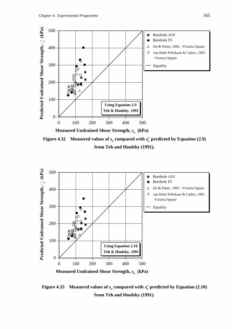
Chapter 4. Experimental Programme 165
�
�
�
���
8
8
8
8
88
1
1
1111111
133
3
3
33333
333
3
3
3
3
3
3
3
3
0
100
200
300
400
500
0 100 200 300 400 500
Measured Undrained Shear Strength, su (kPa)
Using Equation 2.9
Teh & Houlsby, 1991
�
8
Do & Potter, 1992 - Victoria Square
van Holst Pellekaan & Cathro, 19933
1
Victoria Square
Borehole A10Borehole F5
Equality
Figure 4.32 Measured values of su compared with su* predicted by Equation (2.9)
from Teh and Houlsby (1991).
�
�
�
���
8
8
8
8
88
1
1
1111111
133
3
3
33333
333
3
3
3
3
3
3
33
0
100
200
300
400
500
0 100 200 300 400 500
Measured Undrained Shear Strength, su (kPa)
Using Equation 2.10
Teh & Houlsby, 1991
�
8
Do & Potter, 1992 - Victoria Square
van Holst Pellekaan & Cathro, 19933
1
Victoria Square
Borehole A10Borehole F5
Equality
Figure 4.33 Measured values of su compared with su* predicted by Equation (2.10)
from Teh and Houlsby (1991).

166 Chapter 4. Experimental Programme
Examination of Figures 4.30 to 4.33 indicate that Equation (2.7), repeated here:
( )N I fk r= + −12 2ln (4.3)
yields the best comparison of measured, to predicted, undrained shear strengths.
Furthermore, in almost every case, the predicted undrained shear strength is greater than
that measured. Chandler et al. (1992) conducted a study which involved comparing the
results of driven tube samples of London Clay to block samples. The authors concluded
that the process of driving thin-walled tubes to obtain undisturbed samples of soil
significantly increases the effective stress, leading to over-optimistic estimates of the
undrained shear strength and excessive values of K0. This is confirmed by the results
shown in Figures 4.30 to 4.33.
It is imperative in the study of spatial variability to eliminate as many sources of error as
possible, so that the structure of the spatial variation can be identified and isolated from
other causes of variability. Germaine and Ladd (1988) stated that UU tests on specimens
having varying degrees of disturbance will give misleading indications of spatial
variability, due to bias in the measurements. In addition, Jamiolkowski et al. (1988) stated
that the use of qc to obtain su should be limited to non-fissured clays, without highly
developed macrofabric. Since a consistent level of disturbance between samples cannot be
guaranteed (Chandler et al., 1992) and, as discussed in Chapter 2, the Keswick Clay is
heavily fissured, the conversion of qc measurements to su will introduce further variability
to the measured data. As a result, subsequent analyses of these data will be based directly
on the measured values of qc and fs , not derived values of su .
4.6 SUMMARY
It has been shown that cone factors derived from Equation (2.7), from Baligh (1975), yield
the best comparison of measured, to predicted, undrained shear strengths. However,
considerable scatter still exists: s su*
u between 0.86 to 1.06 for borehole A10; and 1.15 to
1.75 for borehole F5. So that additional uncertainties are not introduced into the measured
data, thereby clouding the spatial variability of the soil mass, subsequent analyses of these
data will not be based on derived values of su; but rather on the measured values of qc and
fs . These analyses are presented in the following chapter.