chapter one 1 definition and scope of...

Chapter one

Lecture supporting material for Adam University students, initially prepared by Negash Wagesho, customized by Ermias Alemu

1

1 DEFINITION AND SCOPE OF IRRIGATION Definition: Irrigation is the science of artificial application of water to the land, in accordance with the crop requirements throughout the crop period for full nourishment of the crops. It is the Engineering of controlling and harnessing the various natural sources of water, by construction of dams & reservoirs, canals & head works and finally distributing the water to agricultural fields. Water is normally supplied to the plants by nature through the rains. However, the total rainfall in a particular area may be either insufficient, or ill-timed. In order to get the maximum yield it is essential to supply the optimum quantity of water and to maintain correct timing of water. This is possible only through systematic irrigation system by collecting water during the periods of excess rainfall and releasing it to the crops as when it is needed. Generally the following are some of the factors that necessitate irrigation. - inadequate rainfall - uneven distribution of Rainfall - increasing the yield of the crops - growing a number of crops - insuring against drought. - growing perennial crops.

1.1 Scope of Irrigation Engineering

Irrigation Engineering is not only confined to the application of water to the land for raising crops. It includes all aspects and problems extending from the watershed to the agricultural fields. It deals with hydrology, river engineering, design and construction of dams, weirs, canals and various other hydraulic and irrigation structures. It also deals with surface and sub surface drainage system, soil reclamation, water-soil-crop relationships. Other allied sciences such as flood control, hydropower, and inland navigation are also studied in IRRIGATION Engineering.

1.2 Various aspects of Irrigation Engineering is: 1. Water resources and hydrology aspect – to locate various water sources and to study the

hydrology of the region. This includes study of meteorology, precipitation, stream flow, floods, river engineering, reservoirs and flood control. The following information are required while designing various irrigation structures.

• The quantity of water that will be available at a reservoir site for storage, • Maximum discharge at a river site, • Reservoir capacity that ensures adequate Quantity of water for various purposes, • Quantity of ground water which can be economically exploited.

2. Engineering Aspect - involves the development of a source of water for irrigation and construction of various irrigation structures. • Dams and water power Engineering • Diversion and Distribution structures • Minor irrigation schemes (well, Tank / Pond, inundation Irrigation).

3. Agricultural aspect – Involves irrigation practice and the study of agricultural

Chapter one


2

characteristics of the land. 4. Management Aspect- deals with successful implementation and efficient management of

engineering aspects and agricultural works.

1.3 BENEFITS & ILL-EFFECTS OF IRRIGATION There are various direct and indirect advantages of irrigation.

- Increase in food production: Irrigation helps in increasing crop yields through controlled and timely supply of water to the crop.

- Optimum benefits: optimal utilization of water is made possible by irrigation. Optimum utilization implies obtaining maximum crop yield with any amount of water. In other words, yield will be smaller for any quantity lesser than or in excess of optimum quantity.

- Elimination of mixed cropping in areas where irrigation is not ensured, generally mixed cropping is adapted. Mixed cropping is growing two or more crops simultaneously in the same field. If the weather condition is not suitable to one of the crops it may be suitable for the other; and thus at least some yield is obtained. Mixed cropping can be adopted when irrigation facilities are not available, but if irrigation is assured it can be eliminated. Mixed cropping is generally not acceptable, because different crops require different types of field preparations and different types of manures, amount of water etc.

- General prosperity: Revenue returns are sometimes quite high and helps in all round development of the country

- Generation of hydroelectric power: cheaper power generation can be obtained on objects primarily designed for irrigation alone. Also falls on irrigation channels can be utilized to generate electricity which may help in industrializing the rural area and so in solving the problem of fuel shortage.

- Domestic water supply:- irrigation helps in augmenting the town water supply where water is available with great difficulty. It also provides water for swimming bathing, cattle drinking etc.

- Facilities of communication: Irrigation channels are generally provided with embankments and inspection roads. These inspection paths provide a good road way to the villagers for walking, cycling or even motoring.

- In land navigation

1.4 Ill-effects of irrigation Ill-effects of irrigation occur only when the scheme is not properly designed and implemented. Most of these are due to excess irrigation water application. Some of the common ill-effects are 1. Water logging

when cultivators apply more water than actually required by the crops, excess water percolates in to the ground and raises the water table. Water logging occurs when the water table reaches near the root zones of the crops. The soil pores become fully saturated and the normal circulation of air in the root zones of the crop is stopped and the growth of the crops is decreased. Thus crop yield considerably reduces. When the water table reaches the ground surface, the land becomes saline.

2. Long term application of pesticides under large scale irrigation system might have a negative influence on soil microbal activities, on the quality of surface and sub surface water resources and the survival of the surrounding vegetation. Irrigation may contribute in various ways to the problem of pollution. One of these is the seepage in to the ground of the nitrates that has been

Chapter one


3

applied to the soil as fertilizer. Sometimes up to 50% of the nitrates applied to the soil sink in to the underground reservoir. The under ground water thus get polluted.

3. Irrigation may result in colder and damper climate causing outbreak of disease like malaria. 4. Irrigation is complex and expensive in itself. Some times cheaper water is to be provided at the

cost of the government and revenue returns are low.

1.5 1.3 IRRIGATION DEVELOPMENT IN ETHIOPIA Ethiopia is the “water tower” of North Eastern Africa. Many rivers arising in Ethiopia are also the sources of the major water resources in neighboring countries. The country is endowed with water resources that could easily be tapped and used for irrigation. Ironically this country is already suffering from food shortage because of the increasing population and chronic drought occurrence in most part of the eastern and northern part of the country. There is an annual food deficit to the extent of 0.5 to 1.0 million tones in the country. During the period from 1984 to 1992 the food aid annually received was around 0.9 to 1.0 tones (World Bank Report), to meet the demand of the ever growing population (over 72 million) The need for utilizing these resources is most urgent, in particular, in areas of the country where the length of the growing period is short and the precipitation is erratic. In Ethiopia, rainfed agriculture contributes the largest share of the total production. However, over the past few decades, irrigated agriculture has become more important. Prior to the mid-1980s, irrigation in Ethiopia was concentrated on the production of commercial crops, principally cotton and sugarcane on large state farms. By 1980 it was estimated that 85,000 ha. Mainly in the Awash valley, had been developed under this form of production. In addition some 65,000 ha of traditional irrigation was estimated to exist. Predominantly in the highlands and developed on the farmer’s own initiative. These schemes were typically small runoff river diversion, with low production levels. During this period government involvement in irrigation concentrated on the state farms and was channeled through various agencies.

1.6 Historical Back Ground • In 1956 water resource development (WRD) was established within Ministry of public works,

with responsibility for undertaking river basin development studies and such a study was completed for the Blue Nile basin. However irrigation development remained concentrated in the Awash valley and in 1962 Awash valley Authority (AVA) was established.

• In 1971 National Water Resources Commission (NWRC) was established. • In 1977 Valleys agricultural development authority (VADA) was created to extend the

development of large scale irrigated agriculture beyond the Awash valley and AVA become part of VADA.

• In 1981 NWRC strengthened to absorb functions of VADA. It comprised four authorities including water resource development authority (WRDA), which became responsible for the study, design, and implementation of water resource development projects including large scale irrigation.

Chapter one


4

The 1984 drought had a considerable impact on Ethiopia’s development policy, and the 1984 Ten-Year perspective plan allocated top priority to agricultural development with objective of achieving self sufficiency in food production, establishing a strategic reserve meeting the raw material requirement of industries and expanding output of exportable agricultural products to increase foreign exchange earnings.

The Water Sector Development programme of MoWR (2002) organizes irrigation schemes in Ethiopia under four different ways with sizes ranging from 50 to 85,000 ha

• Traditional small scale schemes: These includes up to 100 ha in area, built and operated by farmers in local communities. Traditionally, farmers have built small scale schemes on their own initiative with government technical and material support. They manage them in their own users’ associations or committees and irrigate areas from 50 to 100 ha with the average ranging from 70 to 90 ha. A total of 1,309 such schemes existed in 1992 covering an estimated area of 60,000ha.

Water users’ associations have long existed to operate and manage traditional schemes. They comprise about 200 users who share a main or branch canal and further grouped in to several teams of 20 to 30 farmers each.

• Modern communal schemes: schemes up to 200 ha, built by government agencies with farmer participation. Modern communal schemes were developed after the catastrophic drought of the 1973 as a means to improve food security and peasant livelihoods by providing cash incomes through production and marketing of crops. Such schemes are capable of irrigating about 30,000ha of land.

These schemes are generally based on run-of - diversion of streams and rivers and may also involve micro dams for storage. On-farm support from the respective agricultural departments and maintenance of headwork’s by water, mines and energy sections as well as technical support from the authorized irrigation development Bureaus in different regions is giving supports and trying to strengthen the system.

• Modern private schemes: up to 2000 ha, owned and operated by private investors individually, in partnership, or as corporations. Medium to large scale irrigation schemes in Ethiopia are private enterprises. The private estates are the pioneers in the development of medium and large scale irrigation development projects in the upper Awash during the 1950s and 1960s. During the 1990s some private schemes, mostly in the form of limited companies re-emerged with the adoption of market based economic policy but have expanded relatively slowly.

Currently 18 modern private irrigation projects are operating in some form over a total area of 6000 ha in Oromiya, SNNPR, and Afar regions.

• Public Schemes of over 3,000 ha, owned and operated by public enterprises as estate farms. They are recently developed irrigation schemes during the late 1970s. Gode West, Omo Ratti and Alwero- Abobo began late in the 1980s and early in the 1990s but have not yet been completed. Public involvement towards large scale schemes was withdrawn due to government changes and most of such schemes with the exception of Finchaa sugar estate have been suspended. Large scale schemes being operated by public enterprise extend over an area estimated at 61,000 ha. Oromiya

Chapter one


5

and Affar account nearly 87% of all irrigation schemes and about 73% of this is located in Awash valley. The SNNPR and Somali regions contain 9.9 and 3.3 percent respectively, WSDP (2003).

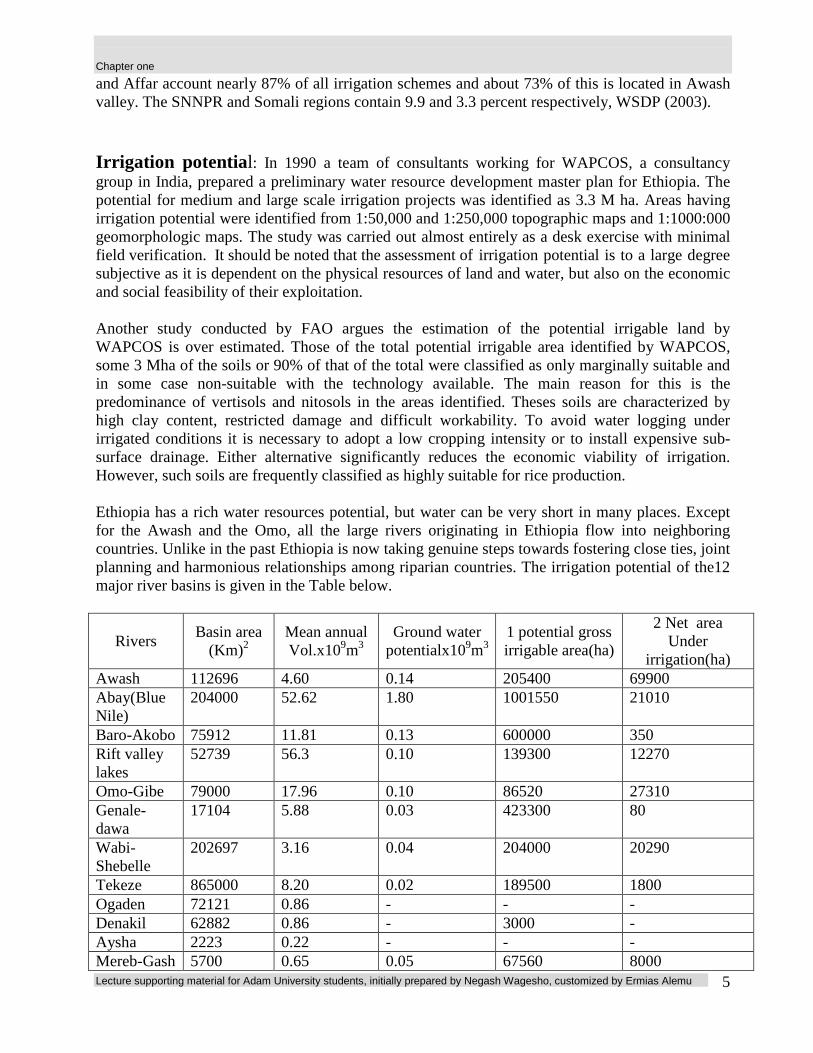
Irrigation potential: In 1990 a team of consultants working for WAPCOS, a consultancy group in India, prepared a preliminary water resource development master plan for Ethiopia. The potential for medium and large scale irrigation projects was identified as 3.3 M ha. Areas having irrigation potential were identified from 1:50,000 and 1:250,000 topographic maps and 1:1000:000 geomorphologic maps. The study was carried out almost entirely as a desk exercise with minimal field verification. It should be noted that the assessment of irrigation potential is to a large degree subjective as it is dependent on the physical resources of land and water, but also on the economic and social feasibility of their exploitation. Another study conducted by FAO argues the estimation of the potential irrigable land by WAPCOS is over estimated. Those of the total potential irrigable area identified by WAPCOS, some 3 Mha of the soils or 90% of that of the total were classified as only marginally suitable and in some case non-suitable with the technology available. The main reason for this is the predominance of vertisols and nitosols in the areas identified. Theses soils are characterized by high clay content, restricted damage and difficult workability. To avoid water logging under irrigated conditions it is necessary to adopt a low cropping intensity or to install expensive sub-surface drainage. Either alternative significantly reduces the economic viability of irrigation. However, such soils are frequently classified as highly suitable for rice production. Ethiopia has a rich water resources potential, but water can be very short in many places. Except for the Awash and the Omo, all the large rivers originating in Ethiopia flow into neighboring countries. Unlike in the past Ethiopia is now taking genuine steps towards fostering close ties, joint planning and harmonious relationships among riparian countries. The irrigation potential of the12 major river basins is given in the Table below.

Rivers Basin area

(Km)2 Mean annual Vol.x109m3

Ground water potentialx109m3

1 potential gross irrigable area(ha)

2 Net area Under

irrigation(ha) Awash 112696 4.60 0.14 205400 69900 Abay(Blue Nile)

204000 52.62 1.80 1001550 21010

Baro-Akobo 75912 11.81 0.13 600000 350 Rift valley lakes

52739 56.3 0.10 139300 12270

Omo-Gibe 79000 17.96 0.10 86520 27310 Genale-dawa

17104 5.88 0.03 423300 80

Wabi-Shebelle

202697 3.16 0.04 204000 20290

Tekeze 865000 8.20 0.02 189500 1800 Ogaden 72121 0.86 - - - Denakil 62882 0.86 - 3000 - Aysha 2223 0.22 - - - Mereb-Gash 5700 0.65 0.05 67560 8000

Chapter one


6

Total 1127312 112.45 2.59 2920130 161010 Note 1= the data extracted from EARO and 2= the data from CSE Ethiopia has not developed irrigation to the potential it has, i.e. according to the availability of physical resources, land and water. At present only a little more than 3% of the irrigable land is currently irrigated both in large and medium scale. The development of irrigated areas in the country has also been unevenly spread. Over 70% of the area developed for irrigation to date is in the Awash river basin. Most of the development has been in the Awash valley, which is the most accessible basin to Addis and has the best infrastructure to support irrigation development.

The spells of drought during the last two decades have led to increased interest in irrigation development. Irrigation is thus expanding in the Wabi-Shebelle and Genale rivers and in the Ziway-Meki area of the rift valley. There are also a number of proposals for further irrigation schemes in several of the other basins including the Omo river, Rift valley lakes and Baro-Akobo. Following the decentralization of governance, there are now a number of regional initiatives to develop irrigation, especially at the small and medium scales, building on existing traditional small-scale irrigation systems, and augmenting them with the diversion of streams and the construction of earth dams. Irrigation development in Ethiopia, as in other countries, has a number of ecological implications because of its impact upon river regimes and downstream flows.

Some of the adverse effects of irrigation development on the environment are: The development of medium and large scale irrigation projects causes a displacement of the indigenous population engaged in pastoral modes of life. Clear examples include the displacement of 60,000 Afar pastoralists from the Amibara irrigation project in the Middle Awash (Mac Donald, 1990) and unspecified number of kereyou pastoralists during the establishment of the Metehara sugar plantation in the upper Awash.

With respect to the use of irrigation for crop production in the highlands, the success has been little. The existence of small scales irrigation schemes by small holders in parts of Shewa, Tigray Harerege, Gojjam, North Omo and few other places are known.

.

2. LAND LEVELING AND FIELD LAYOUT 2.1 Introduction to Land Levelling

Land grading is reshaping of the field surface to a planned grade. It is necessary in making a suitable field surface to control the flow of water, to check soil erosion and provide surface drainage. When uneven land is irrigated, the high spots are watered too little and the low spots too much. This results in uneven crop growth, yield reduction, and loss of water. A properly graded land surface ensures unobstructed smooth flow of water into the land, without eroding the soil and ensuring uniform distribution of water throughout the filed. Land leveling operations may be grouped into three phases:

o Rough grading o Land leveling o Land smoothing

Chapter one


7

Rough grading Is the removal of abrupt irregularities such as mounds, dunes and rings, and filling of pits, depressions and gullies. Land leveling = land grading = land forming = land shaping It requires moving large quantities of earth over considerable distance Land smoothing Leveling operations leaves irregular surfaces due to dumping the loads. These irregularities are removed and a plane surface obtained by land smoothing which is the final operation in land leveling. Criteria for land leveling

Land leveling is influenced by

o the characteristics of the soil profile,

o prevailing land slope,

o rainfall characteristics,

o cropping pattern,

o methods of irrigation,

other specific features of the site including the preference of the farmer

Land clearing Prior to making the land grading survey, it is important to remove heavy vegetative growth from the land. Land clearing consists of removing of some or all the trees, bushes, vegetations, trash and boulders from the area specified for land grading. Layout of fields and irrigation and drainage systems Prior to leveling design, the land development program must be planned so that the location of the filed boundaries, irrigation water supply system, drains and the farm roads are known. The leveling plan for individual fields must provide for furnishing field material or absorbing the excavated earth from those adjacent features. It must also provide fro the proper ratio between excavation and embankment.

2.2 Land Grading Survey and Design

With the field boundaries considered and established, the next step is to survey the area for land leveling design. The general practice is to establish a grid system over the field and set stakes at the grid points (Fig 5.1). Figure 5.1: Grid pattern used for staking a field which is to be graded (A.M. Michael)

Chapter one


8

The usual grid space is 25m in each direction. Other spacing such as 30 * 30m, 20 * 20m, and 15 * 15m are also sometimes used, depending on the nature of the surface relief of the area and the precision required in leveling. Each grid point is at the center of the grid square and represents nearly equal area. For convenience in identification, the row lines are lettered and the column lines numbered. In locating the grid points, the usual practice is to establish two or more base lines in each directions and then to sight in the rest of the stakes. Thus, in Fig. 5.2, line B might first be established by measurements at a distance of one and a half times the grid interval (37.5m), parallel to the south boundary of the field.

Chapter one


9

Figure 5.2: Grid point elevation of the field marked in Fig. 1. Note the contour lines drawn at 10 cm interval on the basis of the grid point elevation

Line 4 and 5 are likewise located at right angle to line B. Line C should also be located by measurement. The stakes are usually of size 1cm by 4cm by 1 m. They should be sharpened and driven into the ground far enough to ensure that they will withstand strong winds. After all the points have been staked, level are run to determine the ground elevation at each stake. The elevations are determined with a dumpy level and a level rod, adopting the usual survey procedures. The first rod reading is made on a bench mark (BM) of known or assumed elevation. Any permanent point on or near the farm may be taken as the bench mark. In case of surveys involving large areas, it is desirable to establish the elevation of the bench mark with reference to mean sea level (MSL) by running a line of differential levels from a point of known elevation, like a near by railway platform or other points.

Chapter one


10

When only a single field is to be surveyed, the first grid point may be taken as the bench mark. Based on the rod readings, the reduced level (RL) of the grid points is computed. The values of RL may be entered in a tabular form or may be indicated directly on the base map at the respective grid points (Figure 5.2). To make the survey information more readily understood and studied, contour lines are drawn at suitable intervals. The contour intervals are usually based on the average land slope. The recommended contour intervals for different ranges of land slopes are as follows:

Land slope range (%) Contour interval (cm) 0 – 1 6 – 15 1 – 2 15 – 30 2 – 5 30 – 60

5 – 10 60 – 150 The contour lines clearly indicate:

o the direction and degree of slope, o ridges, o depressions and o other topographical features.

With the help of contour map the land is divided into fields that can be graded and irrigated individually to the best advantage.

2.3 Land leveling design methods

The basic methods of land leveling design are: 1. plane method 2. profile method 3. plan-inspection method and 4. contour adjustment method

This chapter deals with the plane method in more detail and other methods can be referred from literatures.

Plane Method

The plane method is the most commonly used method of land leveling design. Its use, however, is restricted to those fields where it is feasible to grade the field to a true plane. The following is the procedure for land leveling design. a. Determining the centroid of the filed

o The centroid of a rectangular field is located at the point of intersection of its diagonals. o The centroid of a triangular field is located at the intersection of the lines drawn form its

corners to the mid-points of the opposite sides. o To determine the centroids of irregular field, the area is divided into rectangles and

right angled triangles. The centroid is located by computing moments about two reference lines at right angles to each other.

Chapter one


11

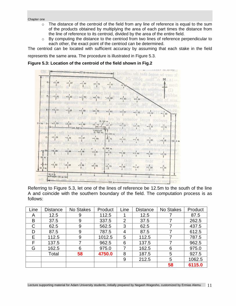
o The distance of the centroid of the field from any line of reference is equal to the sum of the products obtained by multiplying the area of each part times the distance from the line of reference to its centroid, divided by the area of the entire field.

o By computing the distance to the centriod from two lines of reference perpendicular to each other, the exact point of the centriod can be determined.

The centriod can be located with sufficient accuracy by assuming that each stake in the field

represents the same area. The procedure is illustrated in Figure 5.3.

Figure 5.3: Location of the centroid of the field shown in Fig.2

Referring to Figure 5.3, let one of the lines of reference be 12.5m to the south of the line A and coincide with the southern boundary of the field. The computation process is as follows: Line Distance No Stakes Product Line Distance No Stakes Product

A 12.5 9 112.5 1 12.5 7 87.5 B 37.5 9 337.5 2 37.5 7 262.5 C 62.5 9 562.5 3 62.5 7 437.5 D 87.5 9 787.5 4 87.5 7 612.5 E 112.5 9 1012.5 5 112.5 7 787.5 F 137.5 7 962.5 6 137.5 7 962.5 G 162.5 6 975.0 7 162.5 6 975.0 Total 58 4750.0 8 187.5 5 927.5 9 212.5 5 1062.5 58 6115.0

Chapter one


12

The distance of the centriod from the reference line is then obtained by dividing the sum of the products by the total number of stakes, or

m81.89658

4750linereferencethefromcentroidofDistance ==

o Another line of reference may be assumed at 12.5m to the left of the line 1 and the location of the centroid in the east-west direction is computed as 105.603m from the reference line in the same way.

o With the two dimensions, the centroid point is located at (105.603, 81.896). o It may be noted that the centroid point on the x-axis is

105.603 – 87.503 = 18.103m from point D4.

o On the y-axis it is 81.896 – 62.500 = 19.396m from point C5 (Fig. 5.3). b. Determining the average elevation of the field

This is obtained by adding the elevations of all grid points in the field and dividing the sum by the number of points. Thus, in Fig. 5.3,

o the total of the 58 elevations on the grid corners is 98.78m

melevationaverageThe 703.158

78.98 ==

Any plane passing through the centroid at this elevation will produce equal volumes of cut and fill. With the elevation of the centroid known and the downfield grade and cross slope selected, the elevation required at each grid point can be calculated. The desired cut or fill may be computed from the comparison of the original and the proposed elevations. Example Problem 5.1: The topographic survey of a field gave the following elevations (m) at grid points 1 2 3 4 5 A 10.65 10.43 10.07 9.68 9.67 B 10.47 10.42 9.95 9.84 9.75 C 10.32 10.08 9.92 9.65 9.48 D 9.89 9.48 9.67 9.41 9.13 o Calculate the elevation of the centriod of the field. Stakes are to guide the leveling

of this field into a play ground. o Calculate the cut and fill at the grid points. o Compare the quantities of earthwork in cutting and filling Solutions: Total number of stations = 4 * 5 = 20 Total elevations of 20 stations = 197.96

m9.89820

197.96

pointsgridofNumber

pointsgridtheofelevationstheofsumcentroidofElevation ===

Chapter one


13

o Since the field is to be used as a playground, it is to be leveled without any slope in any direction.

o The cuts and fills at various grid points are obtained by subtracting the elevation of

the corresponding grid point from the elevation of the centroid.

o Thus, the cut/fill at grid point A1 is 9.898 – 10.65 = -0.752m. The –sign indicates the cut, while +sign indicates fill. The cuts and fills (in m) at the different grid points are computed which are tabulated below:

1 2 3 4 5

A -0.752 -0.532 -0.172 +0.218 +0.228 B -0.572 -0.522 -0.052 +0.058 +0.148 C -0.422 -0.182 -0.022 +0.248 +0.418 D +0.008 +0.418 +0.228 +0.488 +0.768

Check: ∑ ∑ == mfillcut 228.3

Example Problem 5.2: A topographic survey of a rectangular field was done for planning a land leveling program. Grid points were set at intervals of 25m. The elevations of the points are given below:

Elevation (m) Line 1 Line 2 Line 3 Line 4 Line 5

A 8.26 8.75 9.30 9.52 10.44 B 7.94 8.12 8.90 8.80 9.62 C 7.12 7.86 8.35 8.60 8.42 D 6.74 7.28 7.94 8.16 7.80

o Determine the elevation of the centroid pf the field

o The field is to have a downfield slope of 0.2%. Determine the formation levels at

the grid points and also the amount of cut or fill at each grid point.

Solution

Total number of stations = 20 Sum of the elevations of the 20 stations = 167.92m

mspogridofNumber

spogridtheofelevationstheofsumcentroidofElevation 396.8

20

92.167

int

int ===

The formation levels at the grid points are computed at each grid point with reference to the elevation of the centroid. For example,

o Station A1 is 50m from the north-south line passing through the centroid. o At 0.2% slope, the elevation of this point should be 0.1m below the centroid, or

98.296m. o Similarly, the formation level at each grid point is computed. The results are

tabulated below:

Chapter one


14

1 2 3 4 5 A 8.296 8.346 8.396 8.446 8.496 B 8.296 8.346 8.396 8.446 8.496 C 8.296 8.346 8.396 8.446 8.496 D 8.296 8.346 8.396 8.446 8.496

The cut/fill is computed by subtracting the original elevation of the point from the

formation level at the grid point.

o Thus, at station A1, the cut/fill is 8.296 – 8.260 = +0.036m. The results are

tabulated below:

1 2 3 4 5 A +0.036 -0.404 +0.096 -1.074 -1.944 B +0.356 +0.226 -0.504 -0.354 -1.124 C +1.176 +0.486 +0.046 -0.154 +0.076 D +1.556 +0.066 +0.456 +0.286 +0.696

Check: ∑ ∑ == mfillcut 58.5

c. Compute the slope of the plane of best fit

The slope any line in the x or y direction on the plane which fits the natural ground surface, can be determined by the least squares method. The plane equation can be written as:

( ) CBYAXYXE ++=, ...5.1

Where:

E = elevation of the X, Y coordinate

A, B = regression coefficients

C = elevation of the origin or reference point from the calculations of field topography

using Eq. 5.1

The slope of the best fit line through the average X-direction elevation (Ej) is A, and is

found by:

∑ ∑

∑∑∑

= =

==

−

−

=N

j

N

jjj

N

jj

N

jj

N

jj

NXX

NEXEX

A

1

2

1

2

11

/

/

...5.2

For the best fit slope in the Y-direction, the slope, B, is

Chapter one


15

∑ ∑

∑∑∑

= =

===

−

−=

N

i

N

iii

N

ii

N

ii

N

iii

NYY

NEYEY

B

1

2

1

2

111

/

/

...5.3

Finally, the average field elevation, EF, can be found by summing either Ei or Ej and dividing by the appropriate number of grid rows. This elevation corresponds to the elevation of the field centroid (X,Y). Thus, equation 5.1 can be solved for C as follows:

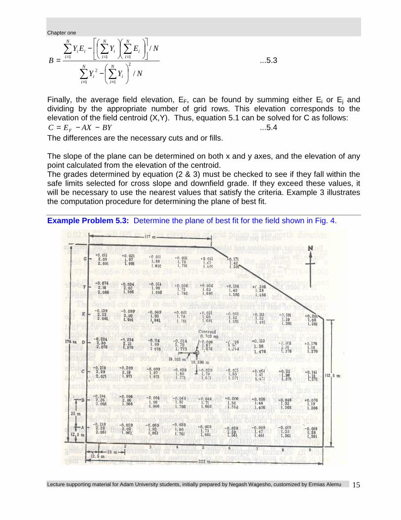
BYAXEC F −−= ...5.4 The differences are the necessary cuts and or fills. The slope of the plane can be determined on both x and y axes, and the elevation of any point calculated from the elevation of the centroid. The grades determined by equation (2 & 3) must be checked to see if they fall within the safe limits selected for cross slope and downfield grade. If they exceed these values, it will be necessary to use the nearest values that satisfy the criteria. Example 3 illustrates the computation procedure for determining the plane of best fit. Example Problem 5.3: Determine the plane of best fit for the field shown in Fig. 4.

Chapter one


16

Figure 5.4: Determination of formation levels cuts and fills for land leveling design of the filed shown in Fig. 5.2, adopting the plane method. Note that each grid point the middle figure shows the original ground elevation, the top figure the cut/fill and the bottom figure the formation level. Solution

o Assuming the southern boundary of the field as the x-axis, the slope of the best fit plane in the y-direction is determined by applying equation 5.3

o The distance of the stations from the x-axis on the different lines and the number of stations on the line are given below:

Line Distance from border, D (m) No. of stations A 12.50 9 B 37.50 9 C 62.50 9 D 87.50 9 E 112.50 9 F 137.50 7 G 162.50 6 Values of E, the elevation of each station are indicated on Fig. 4. Each factor in equation (5.3) is computed as follows:

( ) 125.19228.133.147.159.173.180.193.102.222.25.12 =++++++++=∑ iAEY

( ) 125.57419.132.144.156.171.181.196.106.226.25.37 =++++++++=∑ iB EY

( ) 625.95513.126.141.155.170.180.197.118.229.25.62 =++++++++=∑ iC EY

( ) 375.132710.121.136.154.167.179.199.121.230.25.87 =++++++++=∑ iD EY

( ) 875.165408.119.132.152.165.178.193.102.222.25.112 =++++++++=∑ iE EY

( ) 375.167328.145.163.173.190.102.216.25.137 =++++++=∑ iF EY

( ) 25.173242.161.170.188.197.108.25.162 =+++++=∑ iG EY

⇒ ( )∑ = 75.8109ii EY

475065.16275.13795.11295.8795.6295.3795.12 =×+×+×+×+×+×+×=∑ iY

( )∑ =+++++= 68.9842.161.1.....93.102.222.2iE

⇒( )( )

60.808158

68.984750 =×=∑∑N

EY ii

( ) ( ) 225625004750 22 ==∑ Y

( )389779

58

225625002

==∑N

Yi

Chapter one


17

( ) 5228136)5.162(7)5.137(9)5.112(9)5.87(9)5.62(9)5.37(9)5.12( 22222222 =×+×+×+×+×+×+×=∑ iY

%0212.00002116.0389779522813

60.808175.8109

/

/

1

2

1

2

111 ==−−=

−

−=

∑ ∑

∑∑∑

= =

===

N

i

N

iii

N

ii

N

ii

N

iii

NYY

NEYEY

B

From similar calculations and taking the western boundary of the field as the reference line on the y-axis,

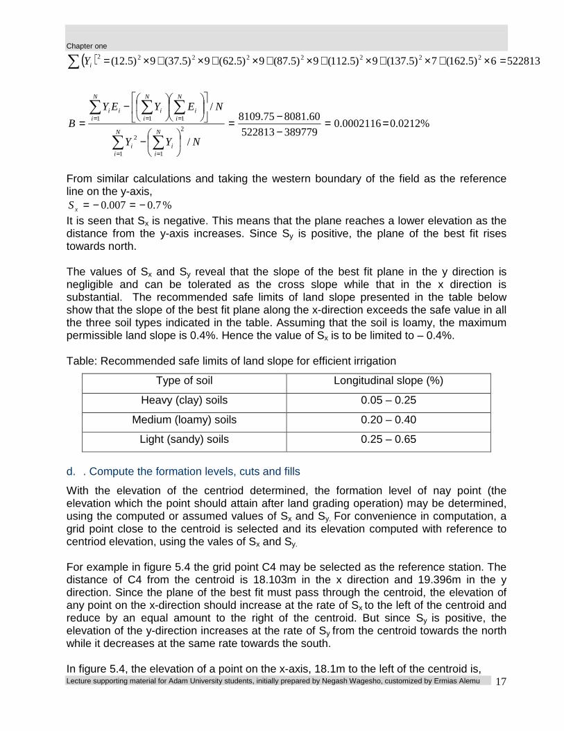
%7.0007.0 −=−=xS It is seen that Sx is negative. This means that the plane reaches a lower elevation as the distance from the y-axis increases. Since Sy is positive, the plane of the best fit rises towards north. The values of Sx and Sy reveal that the slope of the best fit plane in the y direction is negligible and can be tolerated as the cross slope while that in the x direction is substantial. The recommended safe limits of land slope presented in the table below show that the slope of the best fit plane along the x-direction exceeds the safe value in all the three soil types indicated in the table. Assuming that the soil is loamy, the maximum permissible land slope is 0.4%. Hence the value of Sx is to be limited to – 0.4%. Table: Recommended safe limits of land slope for efficient irrigation

Type of soil Longitudinal slope (%)

Heavy (clay) soils 0.05 – 0.25

Medium (loamy) soils 0.20 – 0.40

Light (sandy) soils 0.25 – 0.65

d. . Compute the formation levels, cuts and fills

With the elevation of the centriod determined, the formation level of nay point (the elevation which the point should attain after land grading operation) may be determined, using the computed or assumed values of Sx and Sy. For convenience in computation, a grid point close to the centroid is selected and its elevation computed with reference to centriod elevation, using the vales of Sx and Sy. For example in figure 5.4 the grid point C4 may be selected as the reference station. The distance of C4 from the centroid is 18.103m in the x direction and 19.396m in the y direction. Since the plane of the best fit must pass through the centroid, the elevation of any point on the x-direction should increase at the rate of Sx to the left of the centroid and reduce by an equal amount to the right of the centroid. But since Sy is positive, the elevation of the y-direction increases at the rate of Sy from the centroid towards the north while it decreases at the same rate towards the south. In figure 5.4, the elevation of a point on the x-axis, 18.1m to the left of the centroid is,

Chapter one


18

775.1100

4.0103.18703.1 =×+

Similarly, the decrease in elevation of a point on the y-axis 19.396m from the centroid, towards the south, is

m0039.0100

02.0396.19 =×

Hence the elevation of the grid point C4 = 1.755 – 0.0039 = 1.7711m.

The elevations of all other points on line C can be determined by adding m1.0100

254.0 =×

to each grid points to the left of C4. For example, the elevation of the point C3 is 1.771 + 0.1 = 1.871 and that of C5 = 1.771 – 0.1 = 1.671 and so on. The elevations of the points on line 4 can be obtained by progressively adding

m005.0100

2502.0 =× to the elevations of grid points in the north direction and

subtracting the same amount from the elevations of the preceding grid points in the south direction from C4. Thus, the elevation of B4 = 1.771 – 0.005 = 1.766 m, and that of D4 = 1.771 + 0.005 = 1.776 E4 = 1.776 + 0.005 = 1.781 m and so on Similarly all the design elevations are determined and are shown in figure 5.4.

e. Determine the cut-fill ratio

Experience in land grading with modern earthmoving equipment has shown that the cut-fill ratio should be greater than one. This means that a greater volume of cut than fill must be allowed. Compaction from equipment in the cut area which reduces the volume and also the compaction in the fill area which increases the fill volume needed, are the principal reasons for this effect. Another reason for the need to have additional fill martial results from imperfections in the leveling operation. An argument usually put forth is that on level ground between stakes, the operator has an optical illusion of a dip in the middle, and therefore in filling, crowning often occurs, which requires additional fill material than what is estimated. It is rarely possible to estimate exactly the cu-fill ratio. It usually varies from 1.2 to 1.6. In extreme cases of heavy or light textured soils and deep or shallow excavation, the ration may be as low as. 1.1 and as much as 2.0. In case the soil is composed principally of organic material such as peat or muck, the ration must be about 2.0. The type of soil,

Chapter one


19

quantity of earthwork involved and the type of equipment to be used should be considered in deciding the cut-fill ratio. With the plane method of computing cuts and fills, a settlement correction for the whole field is more convenient to apply. The settlement allowance or amount of lowering of elevation may range from 0.3 to 1cm for compact soils and 1.5 to 4.5 cm for loose soils. It may be noted that a small change in elevation will cause a considerable change in the cut-fill ratio.

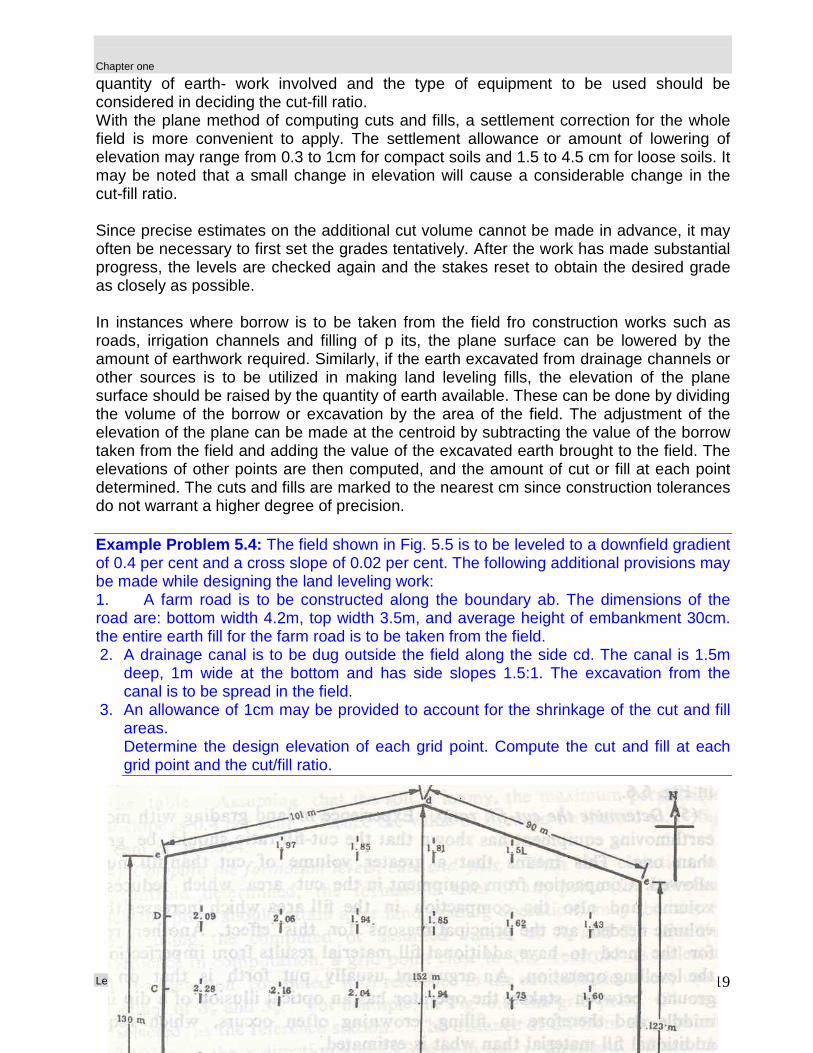
Since precise estimates on the additional cut volume cannot be made in advance, it may often be necessary to first set the grades tentatively. After the work has made substantial progress, the levels are checked again and the stakes reset to obtain the desired grade as closely as possible. In instances where borrow is to be taken from the field fro construction works such as roads, irrigation channels and filling of p its, the plane surface can be lowered by the amount of earthwork required. Similarly, if the earth excavated from drainage channels or other sources is to be utilized in making land leveling fills, the elevation of the plane surface should be raised by the quantity of earth available. These can be done by dividing the volume of the borrow or excavation by the area of the field. The adjustment of the elevation of the plane can be made at the centroid by subtracting the value of the borrow taken from the field and adding the value of the excavated earth brought to the field. The elevations of other points are then computed, and the amount of cut or fill at each point determined. The cuts and fills are marked to the nearest cm since construction tolerances do not warrant a higher degree of precision. Example Problem 5.4: The field shown in Fig. 5.5 is to be leveled to a downfield gradient of 0.4 per cent and a cross slope of 0.02 per cent. The following additional provisions may be made while designing the land leveling work: 1. A farm road is to be constructed along the boundary ab. The dimensions of the road are: bottom width 4.2m, top width 3.5m, and average height of embankment 30cm. the entire earth fill for the farm road is to be taken from the field. 2. A drainage canal is to be dug outside the field along the side cd. The canal is 1.5m

deep, 1m wide at the bottom and has side slopes 1.5:1. The excavation from the canal is to be spread in the field.

3. An allowance of 1cm may be provided to account for the shrinkage of the cut and fill areas. Determine the design elevation of each grid point. Compute the cut and fill at each grid point and the cut/fill ratio.

Chapter one


20

SOLUTION

1) Weighted average elevation of the grid points

.973.128/)43.1...48.250.2( mN

E =++=Σ=

2) The location of the centroid is determined by taking moments about the reference

lines ox and oy. (Note that the reference line ox is drawn parallel to the field boundary

ab and is spaced 15 m away from the field boundary line ab. The line ox is laid at right

angles to oy and is 15m from the field boundary line ae. It is usually advantageous to

locate the reference lines outside the field boundary, and space at least one of it at

half grid spacing from one of the field boundary lines. This is especially important in

the land grading design of fields with irregular boundaries).

Referring to Fig.5.5, the location of the centroid on the plane on the x-axis is

( )m71.85

28

150401269066063060 =×+×+×+×+× from the line oy or 105.0- 5= 90m from

line AE.

Figure 5.5: Plane of field in example 4 with grid point elevations marked

Chapter one


21

3) The slopes of the best fit planes on the x and y-axis are determined by using equation (2 & 3).

Fig. 5.6: Determination of design elevations, cuts and fills of the field shown in Fig. 5,5 adopting the plane method

Chapter one


22

( )( )( ) ( )

( ) ( ) ( )

( )( )

( )

( ) ( )

( ) ( )( )( ) ( ) NYY

NEYEYBb

A

nD

X

NEX

X

EX

NXX

NEXEXAa

ii

iiii

x

j

jj

j

jj

jj

jjjj

/

/)

%458.000458.067500

450.309

226800294300

500.4972050.4663

00.22680028

2520/

000.2943001654...455154

500.497228

25.552520/

00.25201654...755455154

050.4663

97.1...21.230.24509.2...48.250.215

/

/)()(

22

22

2222

22

Σ−ΣΣΣ−Σ

=

−=−=−=−−=∴

==Σ

=×++×+×=Σ

=×=ΣΣ

=×++×+×+×=Σ

=

+++++++=Σ

Σ−Σ

ΣΣ−Σ=

Chapter one


23

( ) ( ) ( )( )

( )( )

( )

( ) ( )

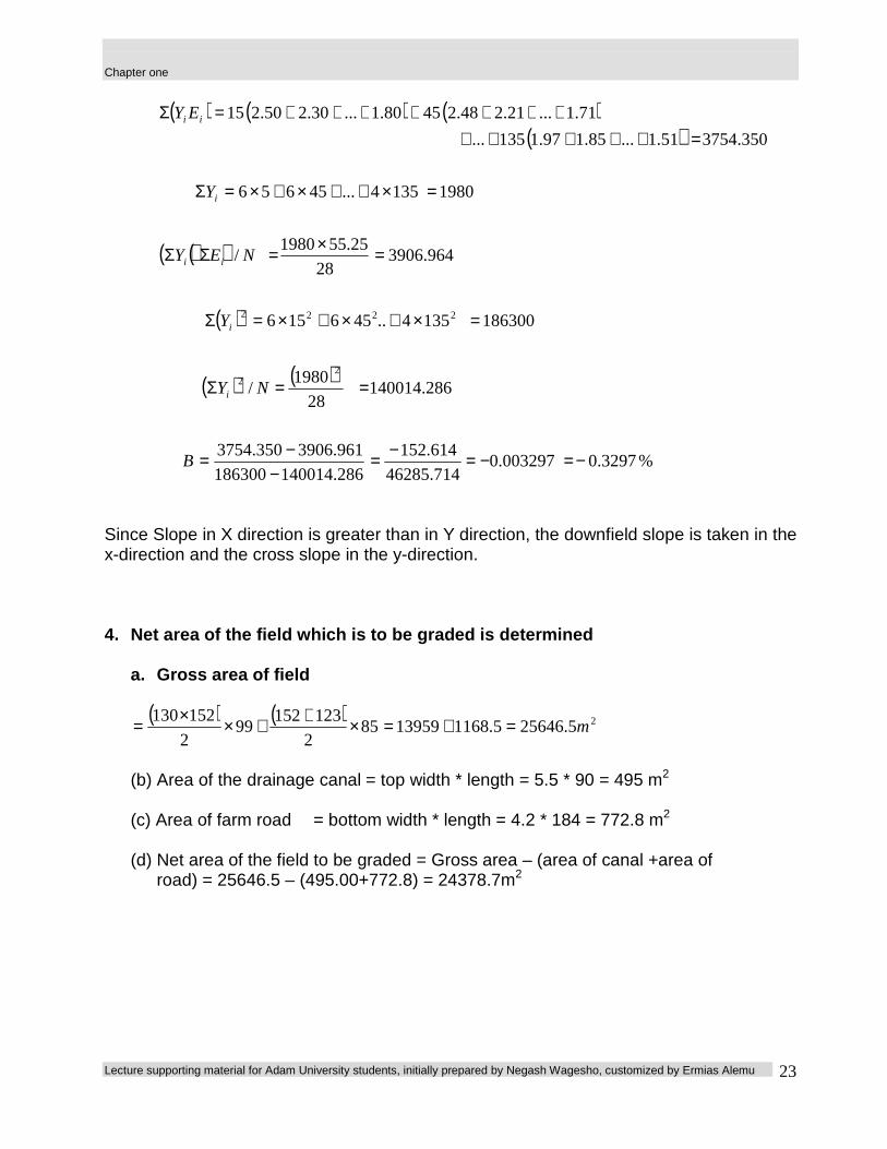
%3297.0003297.0714.46285

614.152

286.140014186300

961.3906350.3754

286.14001428

1980/

1863001354..456156

964.390628

25.551980/

19801354...45656

350.375451.1...85.197.1135...

71.1...21.248.24580.1...30.250.215

22

2222

−=−=−=−

−=

==Σ

=×+×+×=Σ

=×=ΣΣ

=×++×+×=Σ

=++++++++++++=Σ

B

NY

Y

NEY

Y

EY

i

i

ii

i

ii

Since Slope in X direction is greater than in Y direction, the downfield slope is taken in the x-direction and the cross slope in the y-direction.

4. Net area of the field which is to be graded is determined

a. Gross area of field

( ) ( ) 25.256465.11681395985

2

12315299

2

152130m=+=×++××=

(b) Area of the drainage canal = top width * length = 5.5 * 90 = 495 m2 (c) Area of farm road = bottom width * length = 4.2 * 184 = 772.8 m2

(d) Net area of the field to be graded = Gross area – (area of canal +area of

road) = 25646.5 – (495.00+772.8) = 24378.7m2

Chapter one


24

5. Earthwork for road fill and for the excavation of the canal are determined as follows:

b. Volume of earth required for road fill = Cross-sectional area of road

fill x length of road ( ) 252.21218430.0

2

5.32.4m=××+=

Depth of cut required from the entire area of field for the required borrow

mmfieldofareaNet

earthworkofvolume0087.0

7.24378

52.212 ===

c. Volume of excavated earth from drainage canal

= cross- sectional area x length

( ) 275.438905.1

2

15.5m=××+=

Height of earth fills resulting from the spreading of the excavated earth in the net area of field

mfieldofareaNet

excavationofVolume018.0

7.24378

75.438 ===

6. Design elevation of centroid

= Average elevation of field – depth of shrinkage – depth of Borrow + height of excavated earth = 1.973-0.010-0.0087+0.018 = 1.972m

7. With the design elevation of the centroid, the elevation of the grid points and computed so as to obtain a downfield gradient of 0.4 percent and cross slope of 0.02 percent.

The grid point B3 may be taken as the reference point.

( ) ( )

m

BofElevation

037.2005.0060.0972.1

100

71.2502.0

100

154.0972.1

100

6071.8502.0

100

901504.0972.13

=++=

×+×+=

−+−+=

Chapter one


25

The elevation of all grid points on line B, to the left of B3 is obtained by progressively

adding m12.030100

4.0 =× to each succeeding point. Thus, the design elevation of

B2 = 2.037+0.12=2.157 and of B1=2.157+0.12=2.277m.

The elevations of all points to the right of B3 are obtained by subtracting progressively

0.12m from each grid point from the elevation of the previous point on the left. Thus,

the design elevation of

B4=2.037-0.12=1.917m, of B5=1.917-0.12=1.797m and so on.

The design elevations of points on line A can be determined by adding m006.030100

02.0 =×

to the elevation of the corresponding point on line B. similarly, the design elevation of all

points on line C can be determined by subtracting 0.006m from the elevations of the

corresponding points on line B. The elevations of points on line C are obtained by

subtracting 0.006m from the corresponding elevations on line D and so on. The design

elevations, thus obtained, are shown on Fig. 5.6.

8) The cut or fill at each grid point is determined by a comparison of the original

and design elevations.

The values are entered at the entered at the corresponding grid point (Fig. 5.5). The total

cuts and fills fro each column are shown below the corresponding columns. Referring to

Fig.5.5

024.1

608.1

646.1608.1646.1

=

=−

=Σ=Σ

ratiofillCut

FillCut

(Note: If a higher value of the cut-fill ratio is desired, a larger value of shrinkage depth

may be assumed and the problem solved again).

chapter one 1 definition and scope of...

Documents