chapter iv price and volume effects of nifty...
TRANSCRIPT

76
CHAPTER IV
PRICE AND VOLUME EFFECTS OF NIFTY INDEX REVISIONS: A TEST OF PRICE PRESSURE
HYPOTHESIS
4.1 INTRODUCTION
Stock indices play a prominent role in the functioning of stock markets. They reflect
the behaviour of the overall equity market and serve as a benchmark for portfolio
performance. They are also used as an underlying asset in derivative instruments
such as index futures, index options. Further, stock indices aid in passive fund
management by index funds.
Stock indices are regularly monitored and their composition is revised, whenever
required, to ensure that they reflect the true state of the stock market. Owing to the
rapidly changing market conditions and performance of stocks, stock index revisions
have now become a common phenomenon in almost all the markets worldwide.
Stock indices may be revised on account of various reasons. For instance, a stock
currently listed in the index may no longer meet the criteria laid down for a stock’s
existence in the index; hence, the index will be revised and the stock would be
excluded from the index. Indices may be revised also when stocks undergo corporate
actions such as mergers, liquidation, among others.
Stock index revisions can have significant effect on the price and volume of the
stocks undergoing the revision. Examining such effects would help understand the
functioning of the stock markets and the behaviour of market players like index fund

77
managers. It would also aid the investors to profit by framing appropriate investment
strategies.
In the finance literature, two differing views prevail regarding the effects of stock
index revisions. One view, termed as price pressure hypothesis (PPH), argues that
the price effects associated with index revisions are temporary, whereas the other
view asserts that they are permanent, which could be due to varied reasons.
Price pressure hypothesis proposed by Scholes (1972) states that index revisions will
cause a transitory change in the price of stocks that are included to or excluded from
the index, and that the prices will gradually revert to their fundamental values after
the revision. Such price movement is attributed to the heavy trading activity of index
fund managers in response to index revisions.
When an index undergoes revision, index fund15 managers, who track the index,
would rebalance their portfolios by buying the stocks added to the index and selling
those deleted from the index; however, in order to minimize the tracking error, the
fund managers wait until the revision day to update their portfolio. Such trading
activity of index fund managers causes a shift in the demand of the concerned stocks;
the demand for the stocks added to the index increase, while that of the stocks
15 An index fund is a fund that invests in the stocks of the target index in the same proportion in which
these stocks exist in the index. It thereby tries to replicate the index returns and achieve the same
performance as the target index. The performance of such funds is evaluated on the basis of tracking
error. Tracking error refers to the difference between the fund's return and the return of the index
being tracked.

78
deleted from the index decrease. This shift in demand increases the price of the
included stocks and decreases the price of the excluded stocks. Such price increases
(decreases) attract the passive sellers (buyers) who would otherwise not trade. Thus
according to PPH, prior to index revision, price of the stocks added to the index
would increase, while that of stocks deleted from the index decrease.
Once the index revision is over and the index fund managers have updated their
portfolios, the stock prices will revert to their fundamental values, since the heavy
trading by index fund managers would dissipate. Such price reversals after index
revisions enable the passive sellers (buyers) to profit by unwinding their positions if
desired. This way, they are compensated for providing liquidity to the market at the
time of index revisions.
From the above discussion it follows that, according to price pressure hypothesis, the
price and volume effects associated with stock index revisions are temporary. The
prices of stocks added to (deleted from) the index would increase (decrease) prior to
index revision, which would eventually revert to the fundamental values post
revision. The trading volume would temporarily increase for both stock additions
and deletions.
The price and volume effects associated with stock index revisions has been
subjected to extensive empirical examination. The pioneering works on this issue are
those of Harris & Gurel (1986), Shleifer (1986) and Woolridge & Ghosh (1986).

79
Harris & Gurel (1986) investigated the price and volume effects of changes in the
composition of S&P 500 index and reported evidence supporting the price pressure
hypothesis. The study found that stock prices increased by more than three percent
after the announcement of addition and that the stock price increase fully reversed
after two weeks. Further, on the first trading day after the announcement of addition,
large increase in volume is also observed.
On the other hand, evidence refuting price pressure hypothesis was reported by
Shleifer (1986) that examined the price behaviour of stocks included to S&P 500. It
was observed that stock inclusions into S&P 500 were associated with a three
percent announcement date capital gain and that most of it persisted for at least 10 to
20 trading days.
Woolridge & Ghosh (1986) investigated the firms added to and deleted from the
S&P 500 Index and found some evidence in support of price pressure hypothesis.
The study observed temporary stock price effects around deletions. Further,
permanent stock price effect around additions was observed, along with temporary
increase in trading volume.
Since then, various studies have tested price pressure hypothesis. However, majority
of them have tested this issue for the US market and the index that has been largely
used is S&P 500. The results reported by these studies are mixed; some support PPH
whereas others refute it. Similar to Harris & Gurel (1986), the studies that found
evidence in support of PPH are Lynch & Mendenhall (1997), Erwin & Miller
(1998), Dash (2002), Elliott & Warr (2003) and Elliott et al. (2006). On the other

80
hand, similar to Shleifer (1986), studies that have found the price effects of index
revisions to be permanent are Jain (1987), Dhillon & Johnson (1991), Edmister et al.
(1994), Beneish & Whaley (1996) and Chen et al. (2004).
Apart from the above discussed studies that focus on S&P 500 index revisions,
empirical research that examines index revisions pertaining to US market other than
S&P 500 is also available. For instance, using the US stock market indices, viz.,
Dow Jones Industrial and Dow Jones Transportation Averages, Polonchek &
Krehbiel (1994) found that the price and volume effects are inconsistent with price
pressure hypothesis. Similarly, for Dow Jones Industrial Average, Beneish &
Gardner (1995) found that price pressure hypothesis is not supported. In a later
study, Consolandi et al. (2009) for Dow Jones Sustainability Stoxx Index also
documented that index revisions have permanent effects.
Madhavan (2003) examined the effects of revisions made to the US indices, viz.,
Russell 3000 and 2000 indices. The study reports that significant abnormal returns
are observed around the reconstitutions, which could be attributed to temporary price
pressure. Subsequently, Biktimirov et al. (2004) for Russell 2000 index also
supported the price pressure hypothesis. On the contrary, Chen (2006) for US
Russell indices found evidence refuting price pressure hypothesis.
Docking & Dowen (2006) examined the price and volume effects of compositional
changes made to S&P 600 index and found the effects of index revisions to be
temporary. Similar evidence supporting price pressure hypothesis is reported by
Shankar & Miller (2006) for S&P 600 index.

81
Besides US indices, prior empirical research has examined the effects of revisions
made to indices of other markets as well. However, the studies on each market are
very limited. For the Canadian stock market, using Toronto Stock Exchange 300
index, Chung & Kryzanowski (1998) have found evidence in favour of price
pressure hypothesis, whereas Masse et al. (2000) report evidence inconsistent with
price pressure hypothesis.
Chakrabarti (2002) studied the price and volume effects of addition of Indian stocks
to Morgan Stanley Capital International (MSCI) India Standard Index and found
evidence refuting price pressure hypothesis. It was observed that the price increase
associated with stock additions was permanent. Contrary to this, evidence supporting
the price pressure hypothesis was reported by Shu et al. (2004) that examined the
market reaction for Taiwanese listed firms that are added to or deleted from the
MSCI free indices. Further, Chakrabarti et al. (2005) found some evidence of price
pressure in case of additions and deletions of stocks from MSCI Standard Country
Indices for 29 countries.
For the UK market, Gregoriou & Ioannidis (2006) examined the price and volume
effects of stock inclusions and exclusions from FTSE 100 index and reported
evidence inconsistent with price pressure hypothesis. On the other hand, using the
FTSE 100 index changes, Mase (2007) and Mazouz & Saadouni (2007) found the
price effects to be temporary, thereby, lending support to the price pressure
hypothesis. Similar evidence supporting price pressure hypothesis is provided by
Vespro (2006) that examined the compositional changes in FTSE100 index along
with the French indices CAC40 and SBF120.

82
Apart from the above discussed studies, support for PPH is also found in Chan &
Howard (2002) for All Ordinaries Index of Australian stock market, Bechmann
(2004) for Danish blue-chip KFX Index and Doeswijk (2005) for Amsterdam
Exchanges index of Dutch market, while evidence refuting PPH is found in Liu
(2000) for Nikkei 500 Index of Japanese market, Hyland & Swidler (2002) for New
Zealand Stock Exchange’s NZSE40 Index and Wilkens & Wimschulte (2005) for
German Stock indices.
As far as the Indian market is concerned, very few studies have been carried out on
the effects of stock index revisions. The study by Marisetty & Vedpuriswar (2003)
tested the price dynamics around Sensex reconstitutions. The study found that there
is price reversal for additions two days after the effective day, whereas for deletions
there is no such price reversal.
In a later study, Kumar (2007) examined the effects of revisions made to Nifty index
and Junior Nifty index. It is found that, for addition (deletion) of stocks to (from)
Nifty Index, the stock prices significantly increased (decreased) on the effective day,
which reverted after about a week’s time; no abnormal volumes were observed
around the effective day. Such reactions were, however, not observed in the case of
Junior Nifty revisions. The price reactions associated with Nifty revisions provide
some support for PPH, but the lack of abnormal volume in the effective day window
makes this support less forceful.
From the review of literature, it is evident that the validity of price pressure
hypothesis has been extensively investigated by the extant studies. However, in the

83
Indian market, very few studies have focused on this issue. Of these studies, the
study by Marisetty & Vedpuriswar (2003) has examined only the price effects.
Kumar (2007) has examined both the price and volume effects of index revisions;
however, the conclusions drawn by the study regarding price pressure hypothesis are
not emphatic. In this chapter, an attempt has thus been made to test whether PPH
holds good in the Indian market by examining both the price and volume effects of
S&P CNX Nifty revisions.
4.2 METHODOLOGY
To test the validity of PPH in the Indian market, event study methodology, as
described in Wilkens & Wimschulte (2005), is employed and the impact of inclusion
(exclusion) of a stock to (from) Nifty index on the price and volume of the stock is
examined. The event study method enables to estimate and draw inferences about the
impact of a particular event on the behaviour of stocks under consideration. The
event under consideration, here, is the inclusion or exclusion of a stock from Nifty.
The basic terminology of event study is discussed below:
» Event Day: Event day is the day on which the event under consideration
occurs. In this study, the effective day of index revision i.e. the day on which
a stock is included to or excluded from Nifty is the event day and is denoted
as day ‘0’.
» Event Period: Event period is the period over which a particular event is
expected to have an impact on the stock under consideration. Event period
includes the event day and some days prior to and after the event day. The

84
event period for this study consists of the event day and 10 days prior to and
10 days after the event day i.e. -10,…,-1,0,+1,…,+10.
» Estimation Period: Estimation period is the period that is used to obtain the
values of expected return (volume). The estimation period for this study starts
from 170 days prior to and ends at 51 days prior to the announcement day
(AD) of the event i.e. AD-170 to AD-51.
4.2.1 PRICE EFFECTS OF INDEX REVISIONS
To assess the impact of index revisions on the prices of concerned stocks, abnormal
returns are computed. Abnormal return (AR) of a stock is the difference between the
stock’s observed return and its expected return. Observed return is the actual return
observed, whereas expected or normal return is the return that should have been
observed had the event had not taken place.
In this study, abnormal returns are computed using three methods viz., mean
adjusted model, market adjusted model and market model. In each of these models,
the observed return of stock i on day t (��,�) is computed as
��,� = �� � ��,���,���� (4.1)
where ��,� is the price of stock i on day t; ��,��� is the price of stock i on day t-1; i =
1,2,…..,N; N = no. of sample stocks.

85
Each of the three methods differs the way in which the expected return is computed.
The computation of abnormal return under each of the three methods is discussed
below.
(i) Mean Adjusted Model
Under this model, abnormal return of stock i on day t (���,�) is computed as
���,� = ��,� − (��) (4.2)
where ��,� is the observed return of stock i on day t; (��) is the expected return of
stock i; i = 1,2,….,N; N = no. of sample stocks; t = -10,…,0,…,+10.
The expected return of stock i [(��)] is computed as the average of the observed
returns of stock i during the estimation period,
(��) =1
120 ��,������
������
(4.3)
where ��,� is the observed return of stock i on day s; i = 1,2,….,N; N = no. of sample
stocks.
The abnormal return specified in equation (4.2) thus becomes,
���,� = ��,� −1
120 ��,������
������
(4.4)

86
(ii) Market Adjusted Model
In this model, the expected return of stock i on day t [(��,�)] is equal to the market
return on day t (��,�) i.e.
(��,�) = ��,� (4.5)
where i = 1,2,….,N; N = no. of sample stocks; t = -10,…,0,…,+10.
Therefore, the abnormal return is,
���,� = ��,� − ��,� (4.6)
(iii) Market Model
The market model assumes a linear relationship between return of a stock and the
market return, as shown in equation (4.7):
��,� = �� + ����,� (4.7)
where ��,� is the return of stock i on day t; ��,� is the market return on day t; �� is the
market model constant; �� is the slope coefficient.
For each stock i, using the stock’s return and the market return during the estimation
period, the relationship in equation (4.7) is estimated and the parameters �� and �� are obtained. Then, using these parameters, the expected return of stock i on day t
[(��,�)] is computed as,
(��,�) = �� + ����,� (4.8)

87
where �� and �� are the parameters estimated using the returns of stock i and that of
the market during the estimation period; ��,� is the market return on day t; i =
1,2,….,N; N = no. of sample stocks; t = -10,…,0,…,+10.
Abnormal return is then computed as,
���,� = ��,� − (��,�) (4.9)
After calculating the abnormal returns, the mean abnormal return (MAR) is computed
to draw an overall inference about the impact of the event on stock prices. MAR on
day t ( ���) is obtained as the average of abnormal returns of the sample stocks on
day t, i.e.
��� =1����,�
��
(4.10)
where ���,� is the abnormal return of stock i on day t; i = 1,2,…,N; N = no. of sample
stocks; t = -10,…,0,…,+10.
In order to draw inference about the impact of the event over multi-period interval,
cumulative abnormal returns (CAR) are computed. CAR over period [t1,t2] is
obtained as the sum of mean abnormal returns on each day during that period.
�����,�� = ���
��
���
(4.11)
where ��� is the mean abnormal return on day t.

88
4.2.2 VOLUME EFFECTS OF INDEX REVISIONS
To assess the impact of index revisions on the volume of stocks undergoing the
revision, abnormal volumes are computed. As a proxy for trading volume, no. of
shares traded is considered. The trading volume of stock i on day t (��,�) is log
transformed as ��(1 + ��,�). Similarly, the trading volume of market on day t (��,�)
is log transformed as ��(1 + ��,�).
Abnormal volume (AV) is computed employing three methods viz., mean adjusted
model, modified Harris/Gurel model and market model.
(i) Mean Adjusted Model
Under this model, the expected volume of stock i [(��)] is computed as the average
of the trading volume of stock i during the estimation period
(��) =1
120 ��(1 + ��,�)
�����
������
(4.12)
where ��,� is the volume of stock i on day s; i = 1,2,….,N; N = no. of sample stocks.
The abnormal volume of stock i on day t (���,�) is then computed as
���,� = ���1 + ��,�� − (��)
i.e.

89
���,� = ���1 + ��,�� −1
120 ��(1 + ��,�)
�����
������
(4.13)
where ��,� is the volume of stock i on day t; i = 1,2,….,N; N = no. of sample stocks; t
= -10,…,0,…,+10; ��,� is the volume of stock i on day s.
(ii) Modified Harris/Gurel Model
Under this model, the abnormal volume of stock i on day t (���,�) is computed as
���,� = �� � 1 + ��,�1 + ��,�
� − 1
120 ���1 + ��,�
1 + ��,�
������
������
(4.14)
where ��,� is the volume of stock i on day t; i = 1,2,….,N; N = no. of sample stocks; t
= -10,…,0,…,+10; ��,� is the market volume on day t; ��,� is the volume of stock i
on day s; ��,� is the market volume on day s.
(iii) Market Model
Abnormal volume of stock i on day t (���,�), in this model, is computed as
���,� = ���1 + ��,�� − (�� + ����(1 + ��,�)) (4.15)
where ��,� is the volume of stock i on day t; i = 1,2,….,N; N = no. of sample stocks; t
= -10,…,0,…,+10; ��,� is the market volume on day t; �� and �� are the parameters
obtained by estimating the following relation:

90
���1 + ��,�� = �� + ����(1 + ��,�) (4.16)
where ��,� is the volume of stock i on day s; i = 1,2,….,N; N = no. of sample stocks; s
= AD–170 to AD–51; ��,� is the market volume on day s.
After calculating the abnormal volumes, the mean abnormal volume on day t ( ���) is computed to draw an overall inference about the impact of the event on trading
volume. ��� is obtained as the average of the abnormal volumes of sample stocks
on day t, i.e.
��� =1����,�
��
(4.17)
where ���,� is the abnormal volume of stock i on day t; i = 1,2,….,N; N = no. of
sample stocks; t = -10,…,0,…,+10.
Testing for statistical significance
The statistical significance of ��� under each of the three models is tested using
the following test statistic
�����=
����̂( ��) (4.18)
where �̂� ��� is the standard deviation of MAR’s of estimation period computed as

91
�̂� ��� =�∑ � ��� −
1120
∑ ��������
������������
������
119
�
(4.19)
where ��� is the �� on day u; ��� is the �� on day v.
The statistical significance of �����,�� under each of the three models is tested using
the following test statistic
������,��=
�����,���̂� ������ − �� + 1 (4.20)
where �̂� ���is the standard deviation of MAR’s of estimation period as specified
in equation (4.19).
The test statistics in equations (4.18) and (4.20) follow student t-distribution with
119 degrees of freedom. The test statistic to test the statistical significance of MAV is
analogous to that of MAR.
4.2.3 HYPOTHESISED PRICE AND VOLUME EFFECTS OF INDEX REVISIONS AS PER PPH
This section discusses the hypothesized price and volume effects of index revisions
around the effective day, as per PPH. As discussed in section 4.1, when index
revisions occur, index fund managers rebalance their portfolios so as to replicate the
index. However, in order to minimize the tracking error of their portfolios, fund
managers wait until the revision day to rebalance their portfolios. PPH asserts that
such trading activity of fund managers will result in price increase on the effective

92
day for stocks added to the index and price drop for those deleted from the index.
Such price changes will result in abnormal returns on the effective day of revision.
Thus, the null hypotheses with respect to the price effects of Nifty revisions are:
H0pa: There is no abnormal return on the effective day for stocks added to Nifty
H0pd: There is no abnormal return on the effective day for stocks deleted from Nifty
Since index fund managers concentrate their trading on the effective day of index
revision, it is expected that there will be abnormal trading volume on the effective
day, both for stock additions and deletions. The null hypotheses with respect to the
volume effects of Nifty revisions are:
H0va: There is no abnormal trading volume on the effective day for stocks added to
Nifty
H0vd: There is no abnormal trading volume on the effective day for stocks deleted
from Nifty
As per PPH, once index revision is over and index fund managers have updated their
portfolios, the stock prices will revert to their fundamental values. This implies that
price effects observed on the effective day are temporary, and hence, abnormal
returns observed on the effective day should revert post index revision. To test this,
the following null hypotheses are framed.
H0ra: There are no abnormal returns in the post effective day period for stocks added
to Nifty
H0rd: There are no abnormal returns in the post effective day period for stocks
deleted from Nifty

93
4.3 EMPIRICAL RESULTS
The initial sample comprised of the revisions made to S&P CNX Nifty index during
the period September 1996 to September 2010. During this period, there were 61
stock inclusions and 61 stock exclusions. Of this initial sample, those stocks that
were excluded from Nifty on account of corporate actions such as mergers,
amalgamations, demergers etc. were removed.
From the resulting sample, revisions that did not meet the following criteria were
removed:
1. Announcement date should be available for the revision
2. The stock undergoing the revision should not have undergone any other
corporate events, such as mergers, rights issue, bonus issue, stock split,
dividend payment and buy-back of shares, in the respective event and
estimation period
3. For a stock that is included or excluded more than once, it is required that the
event period and estimation period corresponding to each of its events do
not overlap with either the event period or estimation period of its other
events
This screening yielded a sample of 32 inclusions and 32 exclusions. Of this sample,
those stocks that did not have price and volume data over their respective event and
estimation period were removed, which yielded a final sample of 24 inclusions and
31 exclusions16.
16 List of these inclusions and exclusions is provided in Appendix IV-A.

94
Data on firms included and excluded from Nifty along with the respective effective
date and announcement date of revision, the daily closing prices and number of
shares traded of sample stocks, and the daily closing prices and number of shares
traded of Nifty index are collected from Prowess database of Centre for Monitoring
Indian Economy (CMIE) and the official website of NSE17.
4.3.1 PRICE EFFECTS OF NIFTY REVISIONS
In this section, by way of calculating abnormal returns18, the price effects associated
with Nifty index revisions around the effective day of revision are examined. The
price effects around the effective day for stocks added to Nifty are reported in table
4.1. It presents the mean abnormal returns and cumulative abnormal returns under
each of the three models.
17 www.nseindia.com
18 The analysis is carried out in Eviews.

95
Table 4.1: Price effects around the effective day for stock additions to Nifty
N = 24 Mean adjusted model Market adjusted model Market model
Day MAR (%) t-stat
CAR (%) t-stat
MAR (%) t-stat
CAR (%) t-stat
MAR (%) t-stat
CAR (%) t-stat
-10 0.22 0.26 0.22 0.26 0.25 0.45 0.25 0.45 0.06 0.11 0.06 0.11
-9 0.25 0.29 0.46 0.39 -0.34 -0.60 -0.09 -0.11 -0.38 -0.70 -0.32 -0.41
-8 0.25 0.30 0.71 0.49 -0.46 -0.82 -0.55 -0.56 -0.56 -1.02 -0.88 -0.93
-7 0.70 0.83 1.41 0.84 0.24 0.42 -0.31 -0.28 -0.08 -0.14 -0.96 -0.87
-6 0.11 0.13 1.52 0.81 0.35 0.62 0.03 0.03 0.16 0.29 -0.80 -0.65
-5 -0.25 -0.30 1.26 0.62 0.00 -0.01 0.03 0.02 -0.10 -0.19 -0.90 -0.67
-4 -0.89 -1.06 0.38 0.17 -0.44 -0.79 -0.41 -0.28 -0.49 -0.90 -1.40 -0.96
-3 -0.14 -0.17 0.23 0.10 -0.01 -0.02 -0.43 -0.27 -0.02 -0.03 -1.41 -0.91
-2 -1.57 -1.88* -1.34 -0.53 0.75 1.33 0.32 0.19 1.08 1.97* -0.33 -0.20
-1 0.21 0.26 -1.12 -0.43 -0.03 -0.06 0.29 0.16 -0.10 -0.19 -0.44 -0.25

96
0 2.20 2.63*** 1.08 0.39 1.54 2.74*** 1.83 0.98 1.46 2.67*** 1.02 0.56
1 -1.08 -1.29 0.00 0.00 0.09 0.15 1.92 0.99 0.08 0.15 1.11 0.58
2 -0.14 -0.17 -0.14 -0.05 -0.36 -0.65 1.56 0.77 -0.57 -1.03 0.54 0.27
3 -0.56 -0.67 -0.70 -0.22 -0.61 -1.08 0.95 0.45 -0.68 -1.24 -0.14 -0.07
4 -0.33 -0.40 -1.03 -0.32 0.06 0.10 1.01 0.46 -0.01 -0.01 -0.15 -0.07
5 0.95 1.14 -0.08 -0.02 0.37 0.65 1.37 0.61 0.01 0.01 -0.14 -0.06
6 0.06 0.07 -0.02 -0.01 0.08 0.14 1.45 0.63 0.08 0.14 -0.06 -0.03
7 1.01 1.21 0.99 0.28 0.53 0.95 1.98 0.83 0.36 0.65 0.29 0.13
8 0.48 0.58 1.47 0.40 0.64 1.14 2.62 1.07 0.49 0.90 0.78 0.33
9 -0.92 -1.10 0.56 0.15 -0.61 -1.09 2.01 0.80 -0.70 -1.28 0.08 0.03
10 0.18 0.21 0.73 0.19 0.02 0.04 2.03 0.79 -0.04 -0.07 0.05 0.02
Note: MAR denotes Mean Abnormal Return; CAR denotes Cumulative Abnormal Return; day ‘0’ denotes the event day i.e. the effective day of stocks’ addition to Nifty index; *** and * denotes significance at 1% and 10% respectively

97
As shown in table 4.1, on day ‘0’ i.e. the effective day of stock additions to Nifty,
significant positive mean abnormal returns of 2.20%, 1.54%19 and 1.46%20 are
observed, under the mean adjusted model, market adjusted model and market model
respectively. This finding leads to the rejection of the null hypothesis H0pa, which
implies that stocks added to Nifty experience significant positive abnormal returns
on the effective day of addition.
Significant mean abnormal returns are observed also on day ‘-2’ under the mean
adjusted model and the market model. Other than this, significant mean abnormal
returns are not observed on any day in the pre-event period. Further, in the pre-event
period, no significant cumulative abnormal returns are observed. In the post-event
period, neither mean abnormal return nor cumulative abnormal return is found to be
significant on any day.
Thus, the results of table 4.1 indicate that stocks added to Nifty experience
significant positive price effect on the effective day of addition.
Table 4.2 presents the price effects around the effective day for stocks deleted from
Nifty. It reports the mean abnormal returns and cumulative abnormal returns under
each of the three models.
19 This value is exactly the same as reported by Liu (2000) for stocks added to Nikkei 500.
20 This value is almost equal to the one reported by Kumar (2007) for stocks added to Nifty.

98
Table 4.2: Price effects around the effective day for stock deletions from Nifty
N = 31 Mean adjusted model Market adjusted model Market model
Day MAR
(%) t-stat CAR
(%) t-stat MAR
(%) t-stat CAR
(%) t-stat MAR
(%) t-stat CAR
(%) t-stat
-10 0.21 0.28 0.21 0.28 0.26 0.53 0.26 0.53 0.36 0.77 0.36 0.77
-9 1.20 1.61 1.41 1.33 0.34 0.69 0.61 0.86 0.51 1.09 0.87 1.31
-8 0.78 1.05 2.19 1.69* 0.37 0.75 0.98 1.14 0.32 0.68 1.19 1.46
-7 -0.13 -0.17 2.06 1.38 -0.94 -1.87* 0.05 0.05 -0.95 -2.03** 0.24 0.25
-6 -0.56 -0.74 1.50 0.90 -0.56 -1.12 -0.51 -0.46 -0.41 -0.88 -0.17 -0.17
-5 0.67 0.90 2.17 1.19 0.78 1.56 0.26 0.22 0.86 1.84* 0.69 0.60
-4 -0.87 -1.16 1.31 0.66 -0.68 -1.37 -0.42 -0.32 -0.40 -0.86 0.29 0.23
-3 -0.03 -0.04 1.28 0.61 -0.02 -0.04 -0.44 -0.31 0.03 0.05 0.31 0.24
-2 -2.26 -3.02*** -0.98 -0.44 -0.48 -0.96 -0.92 -0.61 -0.21 -0.44 0.11 0.08
-1 0.29 0.39 -0.69 -0.29 0.30 0.60 -0.62 -0.39 0.25 0.52 0.35 0.24

99
0 -0.21 -0.28 -0.90 -0.36 -1.38 -2.76*** -2.00 -1.21 -1.34 -2.84*** -0.98 -0.63
1 -0.54 -0.73 -1.44 -0.56 0.32 0.65 -1.67 -0.97 0.51 1.09 -0.47 -0.29
2 -0.22 -0.29 -1.66 -0.61 -0.45 -0.91 -2.13 -1.18 -0.35 -0.74 -0.82 -0.48
3 -0.80 -1.08 -2.46 -0.88 -0.74 -1.49 -2.87 -1.54 -0.56 -1.19 -1.38 -0.78
4 -0.53 -0.70 -2.99 -1.03 -0.60 -1.20 -3.47 -1.79* -0.31 -0.66 -1.69 -0.93
5 0.94 1.26 -2.05 -0.68 0.28 0.56 -3.19 -1.60 0.39 0.83 -1.29 -0.69
6 -0.20 -0.26 -2.24 -0.73 -0.12 -0.24 -3.31 -1.61 -0.01 -0.01 -1.30 -0.67
7 0.42 0.56 -1.82 -0.57 -0.02 -0.05 -3.33 -1.57 0.11 0.24 -1.18 -0.59
8 0.42 0.57 -1.40 -0.43 0.22 0.43 -3.12 -1.43 0.45 0.96 -0.73 -0.36
9 0.14 0.18 -1.26 -0.38 0.27 0.53 -2.85 -1.28 0.38 0.82 -0.35 -0.17
10 -0.02 -0.02 -1.28 -0.37 -0.10 -0.21 -2.96 -1.29 -0.05 -0.10 -0.40 -0.18
Note: MAR denotes Mean Abnormal Return; CAR denotes Cumulative Abnormal Return; day ‘0’ denotes the event day i.e. the effective day of stocks’ deletion from Nifty index; ***, ** and * denotes significance at 1%, 5% and 10% respectively

100
As is evident from table 4.2, on day ‘0’ i.e. the effective day of stock deletions from
Nifty, significant negative mean abnormal returns of -1.38% and -1.34% are
observed under the market adjusted model and market model respectively. This
finding leads to the rejection of the null hypothesis H0pd, which implies that stocks
deleted from Nifty experience significant negative abnormal returns on the effective
day of deletion.
Significant mean abnormal returns are observed also on day ‘-2’ under mean
adjusted model, day ‘-7’ under market adjusted model and days ‘-7’ and ‘-5’ under
the market model. Other than these days, significant mean abnormal returns are not
observed on any day in the pre-event period. Further, in the pre-event period, except
the cumulative abnormal return on day ‘-8’ under the mean adjusted model, no
significant cumulative abnormal returns are observed. In the post-event period, other
than the cumulative abnormal return on day ‘4’ under the market adjusted model,
neither mean abnormal return nor cumulative abnormal return is found to be
significant on any day.
Thus, the results of table 4.2 indicate that stocks deleted from Nifty experience
significant negative price effect on the effective day of deletion.
4.3.2 VOLUME EFFECTS OF NIFTY REVISIONS
In this section, by way of calculating abnormal volumes21, the volume effects
associated with Nifty index revisions around the effective day of revision are
examined. Table 4.3 reports the volume effects around the effective day for stocks
21 The analysis is carried out in Eviews.

101
added to Nifty. It presents the mean abnormal volumes pertaining to stock additions
to Nifty under each of the three models.
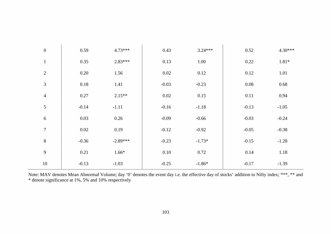
The results of table 4.3 indicate that there are significant positive mean abnormal
volumes on the effective day of addition (day ‘0’) and the day prior to addition (day
‘-1’). Significant positive mean abnormal volume of 0.59, 0.43 and 0.52 is observed,
on the effective day, under the mean adjusted model, modified Harris/Gurel model
and market model respectively. This finding leads to the rejection of the null
hypothesis H0va, which implies that stocks added to Nifty experience significant
positive abnormal trading volume on the effective day of addition.
In the pre-event period, significant positive mean abnormal volumes are observed
also on days ‘-6’ and ‘-4’ under the mean adjusted model and market model. In the
post-event period, under both these models, significant positive mean abnormal
volume is observed on day ‘1’. Further, significant mean abnormal volumes are
observed also on days ‘4’, ‘8’ and ‘9’ under the mean adjusted model and days ‘8’
and ‘10’ under the modified Harris/Gurel model.
Thus, the finding of table 4.3 that stocks added to Nifty experience significant
positive abnormal trading volume on effective day of addition and the day prior to
addition, indicates that there is increased trading volume associated with stock
additions to Nifty.
The volume effects around the effective day for stocks deleted from Nifty are
presented in table 4.4. It reports the mean abnormal volumes pertaining to stock
deletions from Nifty under each of the three models.

102
Table 4.3: Volume effects around the effective day for stock additions to Nifty
N = 24 Mean adjusted model Modified Harris/Gurel model Market model
Day MAV t-stat MAV t-stat MAV t-stat
-10 0.09 0.73 0.01 0.11 0.09 0.73
-9 0.11 0.90 -0.01 -0.08 0.03 0.25
-8 0.15 1.20 0.08 0.63 0.16 1.31
-7 0.13 1.07 -0.02 -0.17 0.07 0.54
-6 0.27 2.17** 0.15 1.12 0.22 1.82*
-5 0.15 1.21 0.06 0.42 0.19 1.55
-4 0.25 1.99** 0.15 1.10 0.21 1.74*
-3 -0.02 -0.20 -0.03 -0.23 0.05 0.43
-2 -0.21 -1.67* -0.08 -0.63 -0.05 -0.43
-1 0.63 5.04*** 0.51 3.88*** 0.60 4.95***
103
0 0.59 4.73*** 0.43 3.24*** 0.52 4.30***
1 0.35 2.83*** 0.13 1.00 0.22 1.81*
2 0.20 1.56 0.02 0.12 0.12 1.01
3 0.18 1.41 -0.03 -0.23 0.08 0.68
4 0.27 2.15** 0.02 0.15 0.11 0.94
5 -0.14 -1.11 -0.16 -1.18 -0.13 -1.05
6 0.03 0.26 -0.09 -0.66 -0.03 -0.24
7 0.02 0.19 -0.12 -0.92 -0.05 -0.38
8 -0.36 -2.89*** -0.23 -1.73* -0.15 -1.28
9 0.21 1.66* 0.10 0.72 0.14 1.18
10 -0.13 -1.03 -0.25 -1.86* -0.17 -1.39
Note: MAV denotes Mean Abnormal Volume; day ‘0’ denotes the event day i.e. the effective day of stocks’ addition to Nifty index; ***, ** and * denote significance at 1%, 5% and 10% respectively

104
Table 4.4: Volume effects around the effective day for stock deletions from Nifty
N = 31 Mean adjusted model Modified Harris/Gurel model Market model
Day MAV t-stat MAV t-stat MAV t-stat
-10 0.00 -0.01 -0.03 -0.15 -0.06 -0.34
-9 0.07 0.36 -0.05 -0.30 -0.03 -0.18
-8 0.13 0.68 0.08 0.46 0.13 0.77
-7 0.00 0.02 -0.07 -0.43 -0.09 -0.54
-6 0.07 0.38 0.02 0.14 -0.02 -0.10
-5 -0.07 -0.39 -0.12 -0.71 -0.14 -0.79
-4 0.07 0.38 0.02 0.09 0.03 0.14
-3 -0.12 -0.63 -0.03 -0.18 0.04 0.22
-2 -0.15 -0.79 0.05 0.32 -0.01 -0.06
-1 0.73 3.83*** 0.67 3.98*** 0.70 4.03***

105
0 0.45 2.37** 0.32 1.87* 0.33 1.93*
1 0.10 0.51 -0.06 -0.35 -0.06 -0.34
2 0.16 0.82 0.05 0.30 0.06 0.32
3 0.03 0.18 -0.12 -0.73 -0.09 -0.50
4 0.10 0.52 -0.06 -0.35 -0.06 -0.37
5 -0.02 -0.09 -0.07 -0.39 -0.07 -0.39
6 0.04 0.23 -0.05 -0.30 -0.04 -0.21
7 0.00 0.02 -0.13 -0.74 -0.10 -0.59
8 -0.04 -0.23 0.00 -0.01 0.10 0.56
9 -0.07 -0.38 -0.19 -1.12 -0.18 -1.02
10 -0.29 -1.51 -0.37 -2.19** -0.39 -2.25**
Note: MAV denotes Mean Abnormal Volume; day ‘0’ denotes the event day i.e. the effective day of stocks’ deletion from Nifty index; ***, ** and * denotes significance at 1%, 5% and 10% respectively

106
The results of table 4.4 indicate that there are significant positive mean abnormal
volumes on the effective day of deletion (day ‘0’) and the day prior to deletion (day
‘-1’). On the effective day of deletion, significant positive mean abnormal volume of
0.45, 0.32 and 0.33 is observed under the mean adjusted model, modified
Harris/Gurel model and market model respectively. This finding rejects the null
hypothesis H0vd, which implies that stocks deleted from Nifty experience significant
positive abnormal trading volume on the effective day of deletion. Besides these two
days, significant abnormal volumes are not observed on any of the days in the event
period, excepting day ‘10’.
Thus, the finding of table 4.4 that stocks deleted from Nifty experience significant
positive abnormal trading volume on effective day of deletion and the day prior to
deletion, indicates that there is increased trading volume associated with stock
deletions from Nifty.
In sum, the volume effects of stock additions along with the corresponding positive
price effect (tables 4.3 and 4.1), indicate that, when stocks are added to Nifty,
demand for those stocks increase leading to a rise in their prices on the effective day
of addition. Similarly, the volume effects of stock deletions together with the
corresponding negative price effect (tables 4.4 and 4.2), reveal that, when stocks are
deleted from Nifty, supply of (demand for) those stocks increase (decrease) leading
to a drop in their prices on the effective day of deletion.

107
4.3.3 NIFTY REVISIONS: TEST OF PRICE PRESSURE HYPOTHESIS
The price effects that occur on the effective day of revision can be either temporary
or permanent. According to PPH, the price effects associated with index revisions
are temporary. Hence, for PPH to hold, the abnormal returns observed on the
effective day of index revision should reverse in the post effective day period. The
insignificant cumulative abnormal returns reported in tables 4.1 and 4.2 seem to
indicate that the positive (negative) price effect associated with stock additions to
(deletions from) Nifty is permanent. In order to further confirm this finding, it is
tested whether the abnormal returns observed on the effective day of Nifty revision
reveres or not in the post effective day period. For this, cumulative abnormal returns
in the various post-effective day windows, both for stock additions and deletions are
computed, the results of which are presented in tables 4.5 and 4.6.
Table 4.5 reports cumulative abnormal returns over various post-effective day
windows, for stocks added to Nifty. It is evident that, under each of the three models,
cumulative abnormal returns are not significant in any of the post-effective day
windows. This finding fails to reject the null hypothesis H0ra, which implies that, for
stocks added to Nifty, there are no abnormal returns in the post effective day period.
This indicates that the abnormal returns observed on the effective day of stock
additions to Nifty do not revert post index revision; hence, the positive price effect
associated with stock additions to Nifty is permanent.

108
Table 4.5: Post-effective day windows’ CAR for stock additions to Nifty
N = 24 Mean adjusted model Market adjusted model Market model
Window CAR (%) t-stat CAR (%) t-stat CAR (%) t-stat
[1,1] -1.08 -1.29 0.09 0.15 0.08 0.15
[1,2] -1.22 -1.03 -0.28 -0.35 -0.48 -0.62
[1,3] -1.78 -1.23 -0.89 -0.91 -1.16 -1.23
[1,4] -2.11 -1.26 -0.83 -0.74 -1.17 -1.07
[1,5] -1.15 -0.62 -0.46 -0.37 -1.16 -0.95
[1,6] -1.10 -0.54 -0.38 -0.28 -1.09 -0.81
[1,7] -0.09 -0.04 0.15 0.10 -0.73 -0.50
[1,8] 0.39 0.17 0.79 0.50 -0.24 -0.15
[1,9] -0.52 -0.21 0.18 0.11 -0.94 -0.57
[1,10] -0.35 -0.13 0.20 0.11 -0.98 -0.56
Note: CAR denotes Cumulative Abnormal Return
109
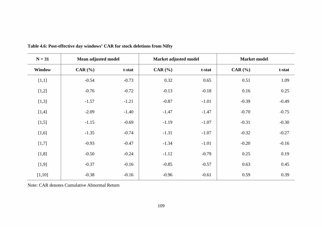
Table 4.6: Post-effective day windows’ CAR for stock deletions from Nifty
N = 31 Mean adjusted model Market adjusted model Market model
Window CAR (%) t-stat CAR (%) t-stat CAR (%) t-stat
[1,1] -0.54 -0.73 0.32 0.65 0.51 1.09
[1,2] -0.76 -0.72 -0.13 -0.18 0.16 0.25
[1,3] -1.57 -1.21 -0.87 -1.01 -0.39 -0.49
[1,4] -2.09 -1.40 -1.47 -1.47 -0.70 -0.75
[1,5] -1.15 -0.69 -1.19 -1.07 -0.31 -0.30
[1,6] -1.35 -0.74 -1.31 -1.07 -0.32 -0.27
[1,7] -0.93 -0.47 -1.34 -1.01 -0.20 -0.16
[1,8] -0.50 -0.24 -1.12 -0.79 0.25 0.19
[1,9] -0.37 -0.16 -0.85 -0.57 0.63 0.45
[1,10] -0.38 -0.16 -0.96 -0.61 0.59 0.39
Note: CAR denotes Cumulative Abnormal Return

110
Cumulative abnormal returns over various post-effective day windows for stocks
deleted from Nifty are reported in table 4.6. Under each of the three models, no
significant cumulative abnormal returns are observed in any of the post-effective day
windows. This finding fails to reject the null hypothesis H0rd, which implies that, for
stocks deleted from Nifty, there are no abnormal returns in the post effective day
period. This indicates that the abnormal returns observed on the effective day of
stock deletions from Nifty do not revert post index revision; hence, the negative
price effect associated with stock deletions from Nifty is permanent.
In sum, the empirical evidence drawn from event study reveal that stocks added to
Nifty experience positive price effect on the effective day of revision, whereas those
deleted experience negative price effect on the effective day. Also, there is increased
trading volume associated with both stock additions and deletions. The lack of price
reversal in the post effective day period indicates that the price effects associated
with stock additions to (deletions from) Nifty are permanent; hence, price pressure
hypothesis does not hold in the Indian market.
4.4 CONCLUSION
Stock index revisions are expected to have a significant effect on the price and
volume of the stocks undergoing the revision. As per price pressure hypothesis,
stock index revisions will cause a transitory change in the price and volume of stocks
that are included to or excluded from the index, and the prices will gradually revert
to their fundamental values after the revision. Such price movement is attributed to
the heavy trading activity of index fund managers in response to index revisions.

111
Extensive research has been carried out on testing the validity of price pressure
hypothesis for different markets. However, in the Indian context, very few studies
have focused on this issue; these studies have either examined only the price effects
or if both price and volume effects have been examined, conclusions drawn by the
study regarding the validity of price pressure hypothesis are not emphatic. This
chapter therefore attempted to test whether price pressure hypothesis holds good in
the Indian market by examining the price and volume effects of S&P CNX Nifty
revisions. For this purpose, stocks added to and deleted from Nifty during the period
September, 1996 to September, 2010 are considered and event study methodology is
employed.
The results of event study indicate that stocks added to Nifty experience positive
price effect on the effective day of revision, whereas those deleted experience
negative price effect on the effective day. There is also increased trading volume
associated with both stock additions and deletions. The lack of price reversal in the
post effective day period indicates that the positive (negative) price effect associated
with stock additions to (deletions from) Nifty is permanent; hence, price pressure
hypothesis does not hold in the Indian market.