chapter iv factors contributing to water-column light

The penetration of sunlight into coastal watersplaces severe constraints on the survival and

spatial distribution of submerged aquatic vegetation.Currently the best estimate for the minimum amountof light required for survival of SAV is as high as 22 percent of incident sunlight for mesohaline andpolyhaline estuarine species (Chapter III).

Light penetration through the water column is con-trolled by the amount and kinds of materials that aredissolved and suspended in the water. Quantitativeunderstanding of the mechanisms by which the variousmaterials affect the transmission of light throughwater forms the basis for setting water quality require-ments for the restoration and protection of SAV. Lightreaching the surface of an SAV leaf is further attenu-ated by attached epiphytic algae and other mineral andorganic detritus adhering to the leaf. Therefore, targetconcentrations of optically active water quality con-stituents must be regarded as minimum requirementsfor SAV survival and growth, which may be modifiedas needed by conditions that promote growth of epi-phytic algae on leaf surfaces (Chapter V).

This chapter documents the development and man-agement application of diagnostic tools for definingthe necessary water quality conditions to develop goalsand management actions for restoring and protectingSAV. The diagnostic tool pertains only to water qualityconditions that influence light attenuation within thewater column. The additional light attenuation occur-ring at the leaf surface due to the accumulation of epi-phytes and associated material is addressed in ChapterV. The process of light attenuation underwater is

briefly summarized. It will be shown that, in spite ofknown nonlinearities, a linear expression relating theattenuation coefficient to water quality concentrationsis all that is justifiable, because of the variability in theoptical properties of the water quality constituents andin the measurements. The diverse origins of sus-pended particulate matter is one factor that increasesthe difficulty of modeling light attenuation over such alarge geographic extent as Chesapeake Bay. The con-tribution of phytoplankton to total suspended solids isestimated to better define the relative roles of nutrientreduction and sediment controls increasing light pene-tration for different locations. The use of a linearmodel of light attenuation to plot a range of waterquality conditions that will result in depth specificattainment of minimum light requirements is thendemonstrated.

WATER-COLUMN LIGHT ATTENUATION

Light underwater is diminished by two processes:absorption and scattering (Kirk 1994). Absorptionremoves light altogether, whereas scattering changesthe direction of propagation. Scattering does notdirectly remove light from the water, but ratherincreases the probability that it will be absorbed, byincreasing the path length or distance that the lightmust travel.

Absorption and scattering interact in a complex andnonlinear manner to govern the attenuation of lightunderwater. The equations governing the propagationof light underwater, called the radiative transportequations, have no exact solution; but several

Chapter IV – Factors Contributing to Water-Column Light Attenuation 35

CHAPTER IIVV

Factors Contributing toWater-Column Light Attenuation

computer programs have been written to solve theequations by various numerical methods (Mobley et al.1993). Despite the complexities of the radiative trans-port equations, field measurements of underwaterirradiance nearly always show a negative exponentialdecay of light with depth. In the absence of strong dis-continuities in water quality, such as nepheloid layers,subsurface chlorophyll a maxima or humic-stained sur-face layers, measurements of photosynthetically activeradiation (PAR, 400-700 nm) are well described by asingle exponential equation of the form

IZ2 = IZ1exp[-Kd(Z2 - Z1)] (IV-1)

where IZ1 and IZ2 are irradiances at depth Z1 and Z2

(Z2>Z1), and Kd is the diffuse attenuation coefficientfor PAR. Several expressions useful for describing thelight available to SAV are easily derived from Equa-tion IV-1. For example, if Z1 represents the surface(depth=0) and Z2 is the maximum depth of SAV colo-nization, Zmax, then the percentage of surface lightpenetrating through the water (PLW) to the plants atdepth Zmax is given by

PLW = exp(-KdZmax)*100 (IV-2).

We denote the minimum PLW required for growth asthe water-column light requirement (WCLR). InEquation IV-2 and the equations that follow, it shouldbe understood that decimal fractions are being usedfor quantities such as PLW and WCLR, expressed aspercentages (i.e. 22 percent=0.22). If WCLR isknown, then the largest diffuse attenuation that wouldpermit growth to depth=Zmax is given by

Kd = ln(WCLR)/Zmax (IV-3).

Expressing Kd in Equation IV-3 as a function of theoptically active water quality parameters forms thebasis for the diagnostic tool for identifying a range ofwater quality conditions necessary for achieving thewater-column light target.

PARTITIONING SOURCES OF WATER-COLUMN LIGHT ATTENUATION

Underwater light is attenuated by water itself and bycertain dissolved and particulate substances. The opti-cally important water quality parameters are coloreddissolved organic matter or yellow substance (Kirk1994), and suspended particulate matter. Suspendedparticulate matter can be further characterized by its

contributions from fixed (i.e., noncombustible) sus-pended solids composed of clay, silt and sand mineralparticles, and volatile (i.e., combustible) suspendedsolids composed of phytoplankton chlorophyll a andnonpigmented organic detritus. Each of the materialshas characteristically shaped light absorption spectra.Because PAR is measured over a wide range of wave-lengths, the spectral dependence of absorption meansthat the effect of one material, for example, phyto-plankton, on light attenuation will depend on the con-centrations of other materials present at the sametime. For this and other reasons related to the non-linearity of the radiative transport equations, the con-cept of a partial attenuation coefficient for the variousoptical water quality parameters is only an approxima-tion, and one that has been criticized (Kirk 1994). Inspite of these known limitations in partitioning the dif-fuse attenuation coefficient into contributions due toindividual components, that approach is adopted herebecause of the need to derive a tool that is simple touse with large amounts of data and can be interpretedby managers unacquainted with the details of radiativetransport theory.

First, the attenuation coefficient for downwelling(moving down through the water) light is expressed asthe sum of that due to water (W) plus dissolvedorganic matter (DOC), phytoplankton chlorophyll a(Chl) and total suspended solids (TSS). Based on theanalyses presented below, it is assumed that attenua-tion due to dissolved matter is relatively constant andmay be included with water itself. We further assumethat the contributions to light attenuation due tochlorophyll a and total suspended solids are propor-tional to their concentrations, so that the diffuse atten-uation coefficient may be written as

Kd = K(W+DOC) + kc[Chl] + ks[TSS] (IV-4)

where K(W+DOC) is the partial attenuation coefficientdue to water plus colored dissolved matter, and kc andks are the specific-attenuation coefficients due, respec-tively, to chlorophyll a and to total suspended solids.By combining equations IV-3 and IV-4, combinationsof chlorophyll a and total suspended solids that justmeet the WCLR may be calculated using:

ln(WCLR)/Zmax =K(W+DOC) + kc[Chl] + ks[TSS]

(IV-5).

36 SAV TECHNICAL SYNTHESIS II

By assuming that K(W+DOC) is constant, Equation IV-6can be used to calculate linear combinations of con-centrations of total suspended solids and chlorophyll athat just meet the WCLR,

[TSS] ={[ln(WCLR)/Zmax]-K(W+DOC)kc[Chl]}/ks

(IV-6).

For a 1-meter colonization depth and PLW equaling22 percent, ln(WCLR)/Zmax=1.51. Parallel lines forother colonization depths are found by dividingln(PLW) in Equation IV-5 by the appropriate value ofZmax. Adjustment of the colonization depth for tidalrange is a simple but important modification pre-sented in Chapter VI.

DIAGNOSTIC TOOL COEFFICIENTS

Application of the diagnostic tool requires values forthree coefficients: the attenuation due to water plusdissolved matter, K(W+DOC), the specific-attenuationcoefficients for phytoplankton chlorophyll, kc, andtotal suspended solids, ks. Initially, coefficients(including a separate specific-attenuation coefficientfor dissolved organic carbon) were estimated by multi-ple linear regression of Kd (dependent variable, calcu-lated from vertical profiles of underwater quantumsensor readings measured by the Chesapeake Bay Phy-toplankton Monitoring Program) against dissolvedorganic carbon, chlorophyll a and total suspendedsolids (independent variables) measured through theChesapeake Bay Water Quality Monitoring Program.Statistical summaries of the measured water qualityparameters at stations for which light profiles weremeasured are reported in Table IV-1, and results of thelinear regressions are given in Table IV-2.

Due to variability in the data, coefficients of determi-nation were generally low, and occasionally (at fivestations for kc) negative specific-attenuation coeffi-cients were calculated. Therefore, coefficients wereselected using a combination of approaches in whichcoefficients estimated by linear regression with theChesapeake Bay Monitoring Program data were firstexamined. The resulting linear regression estimateswere compared with literature values where available,and refined using the optical model of Gallegos(1994), in which individual water quality parameterscan be varied independently. Predictions made withthe refined linear regression were again compared

with measurements made through the ChesapeakeBay Water Quality Monitoring Program to correct foroverall bias.

Water Alone

The attenuation due to water alone is taken to be theintercept of a regression of Kd against the three opti-cal water quality parameters, dissolved organic carbon,chlorophyll a and total suspended solids. Intercepts inthe regressions of Kd against dissolved organic carbon,chlorophyll a and total suspended solids ranged from0.4 to 1.1 m-1 at mainstem Chesapeake Bay WaterQuality Monitoring Program stations, and from 0.6 to3.2 m-1 at tidal tributary Chesapeake Bay Water Qual-ity Monitoring Program stations. In general, these arevery high values and cannot represent the actual atten-uation due to water itself that would occur if all otheroptically active constituents were removed.

Light absorption by pure water varies strongly over thevisible spectrum, being minimal in the blue andincreasing sharply at red wavelengths. Because of thespectral narrowing caused by the selective absorptionof red wavelengths, the attenuation attributable towater itself varies strongly with the depth range con-sidered (Morel 1988). Lorenzen (1972) estimated theattenuation due to water alone to be 0.038 m-1, thoughhis measurements were for deep ocean conditions, inwhich measurements generally commence at depths > 5 meters.

The optical model of Gallegos (1994) with water as theonly factor contributing to attenuation predicts arange of KW from about 0.16 to 0.13 m-1 as the depthis varied from 1 to 3 meters. Though the variation mayseem small, the same model calculates Lorenzen’s(1972) value of 0.038 m-1 for seawater over a 51-meterdepth interval. Thus, in shallow water, the attenuationdue to water itself is not negligible, though muchsmaller than the intercepts estimated by linear regres-sion in Table IV-2. Evidently, the regressions lumpmuch unexplained variance into the intercept.

Dissolved Organic Carbon

Statistically significant coefficients for specific attenu-ation of dissolved organic carbon were obtained atonly two stations, giving specific-attenuation co-efficients of 0.09 and 0.2 m2 g-1 (Table IV-2). The over-all coefficient of determination and accompanying



TABLE IV-1. Statistical summaries of concentrations of optical water quality parameters—chlorophyll,dissolved organic carbon and total suspended solids for Chesapeake Bay Water Quality MonitoringProgram stations at which underwater light measurements were made.

continued

Number of MedianStation Observations Mean Derivation Standard Minimum Maximum

(µg/L)

(mg/L)

(mg/L)

(µg/L)


TABLE IV-1. Statistical summaries of concentrations of optical water quality parameters—chlorophyll,dissolved organic carbon and total suspended solids for Chesapeake Bay Water Quality MonitoringProgram stations at which underwater light measurements were made (continued).

Number of MedianStation Observations Mean Derivation Standard Minimum Maximum

(mg/L)

(mg/L)


TABLE IV-2. Coefficients (an estimate of specific-attenuation coefficient) and intercepts (an estimate ofattenuation due to water alone) estimated by linear regression of diffuse attenuation coefficient, Kd(dependent variable), against concentrations of dissolved organic carbon, phytoplankton chlorophylland total suspended solids. Data from Chesapeake Bay Water Quality Monitoring Program, but limitedto stations at which underwater light measurements were made. ns = not statistically significant,P>0.05.

coefficients for specific-attenuation of total suspendedsolids were anomalously low at these two tidal tribu-tary stations, casting doubt on the reliability of thesevalues.

Only a variable fraction of dissolved organic carbon,referred to as colored dissolved organic matter, con-tributes to light attenuation (Cuthbert and del Giorgio1992). Therefore, the lack of statistically significantcoefficients at most stations is not surprising. Coloreddissolved organic matter absorbs light but does notcontribute appreciably to scattering (Kirk 1994). In thePAR waveband, absorption by colored dissolvedorganic matter is maximal in the blue region of thespectrum and decreases exponentially with wave-length. Optically, the effect of colored dissolvedorganic matter on attenuation is best quantified by theabsorption coefficient of filtered estuary water (0.2 or0.4 mm membrane filter) at a characteristic wave-length, which, by convention, is most often 440 nm(Kirk 1994).

In an effort to quantify the contribution of colored dis-solved organic matter to attenuation, the regression ofGallegos et al. (1990) between absorption coefficient(corrected to 440 nm) and dissolved organic carbonwas incorporated into the model of Gallegos (1994).Water quality conditions for other parameters, chloro-phyll a and total suspended solids, were chosen to rep-resent average conditions for a range of water qualitymonitoring stations along the upper length of themainstem Chesapeake Bay (Table IV-1).

The specific attenuation coefficient of dissolvedorganic carbon calculated by the model varied from0.026 m2 g-1 for upper Bay tidal fresh conditions to0.031 m2 g-1 for lower Bay mesohaline conditions.Concentrations of dissolved organic carbon were sur-prisingly uniform along the axis of the mainstemChesapeake Bay, ranging from about one to six mgliter-1 in the upper Chesapeake Bay to two to nine mgliter-1 at station CB5.2, located in the mainstem Chesa-peake Bay off the mouth of the Potomac River (TableIV-1). The contribution of dissolved organic carbon tolight attenuation can, therefore, be expected to aver-age about 0.07 m-1 and range from about 0.03 to 0.23m-1. The average contribution of dissolved organic car-bon to light attenuation is less than that of water itself(i.e., >0.13 m-1, see above) in shallow systems andtherefore can be expected to be difficult to detect in

monitoring data, which are subject to expected levelsof sampling and analytical error.

Therefore, as discussed above, the effect of dissolvedorganic carbon was incorporated into the regressionfor Kd as a constant term lumped in with the attenua-tion due to water itself. It must be recognized that thisapproximation will not be applicable to tidal tributar-ies with high concentrations of humic-stained water,such as the Pocomoke River. Site-specific approacheswill be needed to tailor the diagnostic tool for such sys-tems, including collection of optically relevant waterquality data, namely absorption by dissolved matter at440 nm (ideally) or color in Pt. units.

A trial value for the combined attenuation due towater and dissolved organic carbon, K(W+DOC), wasdetermined by setting total suspended solids andchlorophyll a concentrations in the model of Gallegos(1994) to zero, and allowing concentrations of dis-solved organic carbon to vary according to a normaldistribution with mean of 2.71 mg liter-1 and standarddeviation of 0.44 mg liter-1, similar to observations atChesapeake Bay Water Quality Monitoring Programstation CB3.3C (Table IV-1). Attenuation due to waterand dissolved organic carbon calculated in this mannervaried from 0.21 to 0.31 m-1 and averaged 0.26 m-1,which was used as a trial value.

Phytoplankton Chlorophyll

Phytoplankton, being pigmented cells (i.e., particles),contribute both to absorption and the scattering oflight. Light absorption by phytoplankton variesstrongly with wavelength. The shape of the in vivoabsorption spectrum of phytoplankton varies withspecies, but generally, peaks occur at about 430 nmand at 675 nm, with a broad minimum in the greenregion of the spectrum (Jeffrey 1981). Because of thisspectral dependence, the contribution of phytoplank-ton to attenuation varies with the depth and com-position of the water (Atlas and Bannister 1980), andto a lesser extent in natural populations, with speciescomposition.

By linear regression on data from the Chesapeake BayWater Quality Monitoring Program, statistically signif-icant estimates for the specific-attenuation coefficientfor chlorophyll a were obtained at 6 of 13 stations(Table IV-2). Two of those were negative values andmust be considered spurious. Significant positive


values ranged from 0.011 to 0.019 m2 (mg Chl)-1. Thisrange compares favorably with values reported in theliterature. For example, Atlas and Bannister (1980)used a fixed specific absorption spectra and calculateda range of the chlorophyll-specific attenuation coeffi-cients near the surface ranging between 0.013 and0.016 m2 (mg Chl)-1. The overall magnitude of thechlorophyll-specific absorption spectrum, however,varies considerably with physiological state, photo-adaptation, and recent history of light exposure of thephytoplankton population. A wider survey of the liter-ature, reviewed by Dubinsky (1980) suggested valuesbetween 0.005 and 0.040 m2 (mg Chl)-1, but most esti-mates range more narrowly between 0.01 to 0.02 m2

(mg Chl)-1 (Lorenzen 1972; Smith and Baker 1978;Smith 1982; Priscu 1983).

Model-generated estimates of kc can be similarly vari-able. The effect of chlorophyll a on Kd is incorporatedin the optical model through the chlorophyll-specificabsorption spectrum. The coefficient of variation inmeasured chlorophyll-specific absorption spectra inthe Rhode River was about 50 percent (Gallegos 1994)and overall range varied by about a factor of four (Gal-legos et al. 1990). When this degree of variability in thechlorophyll-specific absorption spectrum is incorpo-rated into the optical model of Gallegos (1994), calcu-lated kc range from <0.01 to 0.035 m2 (mg chl)-1, withan average of about 0.016 m2 (mg Chl)-1. Therefore, aninitial estimate for kc of 0.016 m2 (mg Chl)-1 waschosen. This value is near the center of the observedrange and is commensurate with the optical waterquality model and literature estimates (Bannister1974; Smith and Baker 1978; Priscu 1983).

Total Suspended Solids

Statistically significant estimates for the specific-attenuation coefficient for total suspended solids wereobtained by the linear regression analysis at all but onestation (Table IV-2). Values for ks ranged from 0.013 to0.101 m2 g-1. Because of the wide range of coefficientsand because the lower values (< 0.05 m2 g-1) were gen-erally associated with lower coefficients of determina-tion (Table IV-2), literature and model-generatedvalues for ks were also examined.

Literature estimates of ks in estuaries tend to clusteraround the middle of the range estimated from theChesapeake Bay Water Quality Monitoring Program

data. For example, Cloern (1987) estimated ks of 0.06m2 g-1 for San Francisco Bay, similar to Malone’s(1976) value for the New York Bight. Pennock (1985)estimated a specific-attenuation coefficient of 0.075m2 g-1 in the Delaware Estuary, similar to two of themainstem Chesapeake Bay water quality stations(Table IV-2). Verduin (1964; 1982 cited in Priscu 1983)found ks averaged 0.12 m2 g-1 for a number of river-dominated freshwater systems, similar to the regres-sion estimate for upper Chesapeake Bay station CB1.1(Table IV-2).

The optical model of Gallegos (1994) accounts for thecombined effects of scattering and absorption by sus-pended particulate matter using the equations of Kirk(1984). As discussed above, scattering contributes tolight attenuation by increasing the path length thatlight travels, thereby increasing the probability ofabsorption. Direct measurement of scattering is diffi-cult; but by fortunate coincidence, the turbidity of awater sample measured in nephelometric turbidityunits (NTU) using commercially available turbidime-ters has been shown to be a good estimate of scatter-ing coefficient in relatively turbid waters, includingestuaries, by a number of authors (Kirk 1981; Oliver1990; Di Toro 1978; Vant 1990). Operationally, this isunderstandable from the manner in which a tur-bidimeter works, i.e., by measuring the intensity oflight scattered at 90 degrees from a beam shoneupward through the bottom of the sample. That theunits of the measurement should scale with scatteringcoefficient is, however, serendipitous (Kirk 1981).

Turbidity has not been routinely monitored in theChesapeake Bay Water Quality Monitoring Program.Measurements in two systems, the Rhode River,Maryland, a Chesapeake Bay tidal tributary, and Chin-coteague Bay, a coastal lagoon on the Maryland-Virginia border, indicate that scattering in bothsystems is strongly dominated by the mass concentra-tion of suspended solids (Figure IV-1A). The relation-ship between turbidity and total suspended solids inthe two systems was nearly identical, despite a muchgreater contribution of chlorophyll a to the suspendedmaterial in the Rhode River (Figure IV-1B) (Gallegos1994). Evidently, phytoplankton contribute to scatter-ing on a dry-weight basis approximately as much asinorganic suspended solids and organic detritus. Thegenerality of these observations is uncertain. It is likelythat relationships as precise as these would be difficultto obtain if the geographic extent or length of time


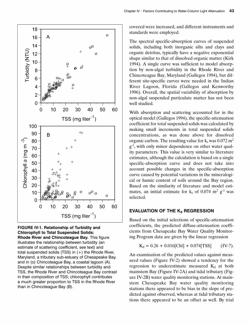
covered were increased, and different instruments andstandards were employed.

The spectral specific-absorption curves of suspendedsolids, including both inorganic silts and clays andorganic detritus, typically have a negative exponentialshape similar to that of dissolved organic matter (Kirk1994). A single curve was sufficient to model absorp-tion by non-algal turbidity in the Rhode River andChincoteague Bay, Maryland (Gallegos 1994), but dif-ferent site-specific curves were needed in the IndianRiver Lagoon, Florida (Gallegos and Kenworthy1996). Overall, the spatial variability of absorption bynon-algal suspended particulate matter has not beenwell studied.

With absorption and scattering accounted for in theoptical model (Gallegos 1994), the specific-attenuationcoefficient for total suspended solids was calculated bymaking small increments in total suspended solidsconcentrations, as was done above for dissolvedorganic carbon. The resulting value for ks was 0.072 m2

g-1, with only minor dependence on other water qual-ity parameters. This value is very similar to literatureestimates, although the calculation is based on a singlespecific-absorption curve and does not take intoaccount possible changes in the specific-absorptioncurve caused by potential variations in the mineralogi-cal or humic content of soils around the Bay region.Based on the similarity of literature and model esti-mates, an initial estimate for ks of 0.074 m2 g-1 wasselected.

EVALUATION OF THE Kd REGRESSION

Based on the initial selections of specific-attenuationcoefficients, the predicted diffuse-attenuation coeffi-cients from Chesapeake Bay Water Quality Monitor-ing Program data are given by the linear regression

Kd = 0.26 + 0.016[Chl] + 0.074[TSS] (IV-7).

An examination of the predicted values against meas-ured values (Figure IV-2) showed a tendency for theregression to underestimate measured Kd at bothmainstem Bay (Figure IV-2A) and tidal tributary (Fig-ure IV-2B) water quality monitoring stations. At main-stem Chesapeake Bay water quality monitoringstations there appeared to be bias in the slope of pre-dicted against observed, whereas at tidal tributary sta-tions there appeared to be an offset as well. By trial


FIGURE IV-1. Relationship of Turbidity andChlorophyll to Total Suspended Solids: Rhode River and Chincoteague Bay. This figureillustrates the relationship between turbidity (an estimate of scattering coefficient, see text) and total suspended solids (TSS) in (+) the Rhode River,Maryland, a tributary sub-estuary of Chesapeake Bay,and in (o) Chincoteague Bay, a coastal lagoon (A).Despite similar relationships between turbidity and TSS, the Rhode River and Chincoteague Bay contrastin their composition of TSS; chlorophyll contributes a much greater proportion to TSS in the Rhode Riverthan in Chincoteague Bay (B).


FIGURE IV-2. Comparison of Measured Kd with Predictions by Linear Regression Model. Comparison ofmeasurements of diffuse attenuation coefficient (Kd) made in the Chesapeake Bay Water Quality Monitoring Program(1986-1996) with predictions made by linear regression against optical water quality parameters. (A) and (B) arepredictions based on initial estimates of coefficients (Equation IV-7); (C) and (D) are predictions based on Equation IV-8, in which attenuation due to water plus dissolved organic carbon and partial attenuation coefficient of totalsuspended solids were adjusted upward. (A) and (C) are data from mainstem Chesapeake Bay stations; (B) and (D) are data from Maryland tidal tributary stations.

and error, predictions were improved by adjusting theestimated K(W+DOC) to 0.32 m-1 and the specific-attenuation coefficient of total suspended solids to0.094 m2 g-1 (Figure IV-2C, -2D), possibly indicatingthat the highest attenuation coefficients are dominatedby times and locations of highest river flows. Thesemodifications result in a final regression model of

Kd = 0.32 + 0.016[Chl] + 0.094[TSS] (IV-8).

Overall, the scatter in these plots indicates that moresophisticated models cannot be considered, given thelimited amount of optical information in the data thatare available. The r2 for the final fits are 0.61 for main-stem Chesapeake Bay stations, and only 0.37 for tidaltributary stations. It is also likely that site-specific coef-ficients for ks and possibly K(W+DOC) will be needed asa future refinement. Present experience with regres-sions on the monitoring data (Table IV-2) indicate thatsite-specific refinements to coefficients will need to becomputed from optical modeling, based on directdetermination of specific-absorption and specific-scattering spectra of total suspended solids from awide range of sites around the Bay.

With these coefficients, Equation IV-6 can be used towrite equations for combinations of chlorophyll a andtotal suspended solids that meet the WCLR for depthsof 0.5, 1.0 and 2.0 meters. For mesohaline and polyha-line habitats where WCLR = 0.22 (22 percent, fromChapter III), the equations are

0.5 m [TSS] = 28.8 0.17[Chl], [Chl] < 169.4 (IV-9a)

1.0 m [TSS] = 12.7 0.17[Chl], [Chl] < 74.7 (IV-9b)

2.0 m [TSS] = 4.65 0.17[Chl], [Chl] < 27.4 (IV-9c)

where the upper bound on [Chl] is the chlorophyll aconcentration at which the predicted [TSS] = 0 forthat depth; that is, higher chlorophyll a concentrationswould result in a prediction of a ‘negative concentra-tion’ for [TSS].

Comparable equations for tidal fresh and oligohalinehabitats are determined by substituting 0.13 (13 per-cent from Chapter III) for WCLR in Equation IV-6,

0.5 m [TSS] = 40.0 - 0.17[Chl], [Chl] < 235 (IV-10a)

1.0 m [TSS] = 18.3 - 0.17[Chl], [Chl] < 107 (IV-10b)

2.0 m [TSS] = 7.45 - 0.17[Chl], [Chl] < 43.8 (IV-10c).

COMPONENTS OF TOTAL SUSPENDED SOLIDS

Total suspended solids consist of the dry weight of allparticulate matter in a sample, including clay, silt andsand mineral particles, living phytoplankton and het-erotrophic plankton, including bacteria and particu-late organic detritus. Therefore, phytoplankton andthe heterotrophic community it supports contribute towhat is measured by total suspended solids. As shownabove, optically it is difficult to distinguish the effect ofparticulate organic matter, including that contributedby phytoplankton, from that of mineral particulates.Nevertheless, it is useful to examine their relative con-tributions to the measurement of total suspendedsolids, since organic particulates (due, in part, to nutri-ent over-enrichment) must be controlled differentlythan mineral particulates (due, in part, to erosion orsediment resuspension). In particular, a reduction inchlorophyll a will be accompanied by a proportionalreduction in total suspended solids due to the dryweight component of phytoplankton. This additionalreduction in total suspended solids needs to be incor-porated into the predicted response of Kd when usingequations (IV-9a-c) for determining the water qualityconditions necessary for achieving the minimum light requirements.

Upon combustion, the particulate organic matter in asample is oxidized, leaving behind the mineral compo-nent and ash of the organic fraction. The fractionremaining after combustion is referred to as fixed sus-pended solids (FSS), and the difference between thetotal and the fixed fraction of suspended solids iscalled total volatile suspended solids (TVSS). The per-centage of total suspended solids that is of organic ori-gin can then be estimated as TVSS/TSS*100.

Fixed suspended solids and total volatile suspendedsolids have been measured at the Virginia tidal tribu-tary and mainstem stations of the Chesapeake BayWater Quality Monitoring Program. At very high con-centrations of total suspended solids, total volatile sus-pended solids appears to approach a relativelyconstant fraction, about 18 percent, of total suspendedsolids (Figure IV-3). The extremely high concentra-tions probably represent flood conditions, and thefraction of total volatile suspended solids in those sam-ples are probably characteristic of the terrestrial soils.At more realistic total suspended solids concentra-tions, i.e., those < 50 mg liter-1, a much wider range inthe percentage of total volatile suspended solids is


observed (Figure IV-3, inset), exceeding 90 percent insome samples.

The relationship between total volatile suspendedsolids and particulate organic carbon shows a greatdeal of scatter (Figure IV-4A) but on average, particu-late organic carbon is about 30 percent of total volatilesuspended solids. This estimate is larger than that ofliving phytoplankton (26 percent) (Sverdrup et al.1942) and lower than that of carbohydrate (37 per-cent). The particulate organic carbon in a sample con-sists of living phytoplankton, bacteria, heterotrophicplankton, their decomposition products, organicdetritus from marshes or terrestrial communities andresuspended SAV detritus. As expected, a plot of par-ticulate organic carbon against phytoplankton chloro-phyll a displays considerable scatter (Figure IV-4B),but during sudden phytoplankton blooms, phytoplank-ton might comprise the major component of carbon ina sample. The ratio of carbon to chlorophyll a in


FIGURE IV-3. Fraction of Total Suspended SolidsLost on Ignition. Fraction of total suspended solids(TSS) that is lost on ignition as a function of TSS. Atconcentrations of TSS < 50 mg liter-1 (inset), the frac-tion of TSS that is volatile varies from 0 to >90 percent.Total volatile suspended solids (TVSS) calculated astotal suspended solids minus fixed suspended solids,that is, the mass remaining after combustion. Fractiontotal volatile suspended solids calculated as total volatilesuspended solids divided by total suspended solids.Data from Chesapeake Bay Water Quality MonitoringProgram, Virginia tidal tributary stations, 1994-1996.

FIGURE IV-4. Relationships of Total VolatileSuspended Solids, Particulate Organic Carbon andChlorophyll. Concentration of total volatile suspendedsolids (TVSS) as a function of particulate organic carbon(POC) for Virginia tidal tributary stations, 1994-1996.Line shows estimate of TVSS as POC/0.3 (A).Relationship of particulate organic carbon to chlorophyllconcentration for Virginia tidal tributary stations (B).Lines bracket approximate contribution of phytoplanktonto POC based on a range of phytoplanktoncarbon:chlorophyll ratios from 20 (dashed line) to 80 mgC (mg chlorophyll)-1(solid line).

phytoplankton varies widely (Geider 1987). A range ofabout 20 to 80 mg C (mg chl)-1 provides a lower boundof most of the points in Figure IV-4B, and this range iswell within the physiological limits of phytoplankton(Geider 1987). Choosing 40 mg C (mg chl)-1—thegeometric mean of 20 and 80–as a representative car-bon:chlorophyll a ratio, and using the 30 percent par-ticulate organic carbon:total volatile suspended solidsratio from Figure IV-4A, the minimum contribution ofphytoplankton chlorophyll a to total volatile sus-pended solids, designated ChlVS, is estimated as

ChlVS = 0.04[Chl]/0.3 (IV-11)

where the 0.04 results from the conversion of µg to mgchlorophyll liter-1. Thus, although the optical effects ofparticulate organic detritus cannot be distinguished fromthat of mineral particles, the minimum contribution ofphytoplankton to the measurement of total suspendedsolids is approximately given by ChlVS. This also impliesthat management action to reduce the concentration ofchlorophyll a at a site will also result in a reduction oftotal suspended solids by an amount approximated byChlVS. The actual reduction may be larger if a substan-tial heterotrophic community and the organic detritusgenerated by it are simultaneously reduced. This obser-vation has significant implications for the implementa-tion of site specific management approaches.

SUMMARY OF THE DIAGNOSTIC TOOL

The exponential decline of light intensity under water(Equation IV-1) allows for the percentage of surfacelight penetrating to a given depth to be written as asimple function of the diffuse attenuation coefficient(Equation IV-2). Equation IV-4 expresses in a general(albeit approximate) way the relationship between thediffuse-attenuation coefficient and the concentrationsof optical water quality parameters. Once the SAVminimum light requirement and the SAV restorationdepth are specified, Equation IV-4 may be rearrangedto predict the concentrations of total suspended solidsand chlorophyll a that exactly meet the water-columnlight requirement (Equation IV-6). Equations IV-9a-cexpress these water quality relationships for mesoha-line and polyhaline regions for three depth ranges, andin terms of the specific-attenuation coefficients esti-mated for Chesapeake Bay from the literature, byoptical modeling and by analysis of data from theChesapeake Bay Water Quality Monitoring Program.Equations IV-10a-c express the same relationships for

tidal fresh and oligohaline regions. Equation IV-11estimates an approximate minimum concentration oftotal suspended solids attributable to phytoplankton.Equation IV-11 is used to better predict the reductionin total suspended solids, and, therefore, the diffuseattenuation expected to occur when the chlorophyll aconcentration is reduced.

APPLICATION OF THE DIAGNOSTIC TOOL

A plot of measured total suspended solids againstchlorophyll a concentrations from a given station inrelation to lines defined by equations IV-9a-c demon-strates the extent to which the water-column lightrequirement is met at that location. In addition, a linerepresenting Equation IV-11 shows the minimum con-tribution of chlorophyll a to total suspended solids atthe location. Three examples from the ChesapeakeBay Water Quality Monitoring Program demonstrateinformation that may be determined by examiningplots of total suspended solids against chlorophyll a inrelation to the restoration depth-based water-columnlight requirements (Figure IV-5).

Suspended Solids Dominant Example

At station CB2.2, located in the upper ChesapeakeBay mainstem near the turbidity maximum, total sus-pended solids dominates the variability in light attenu-ation (Figure IV-5A). The median water qualityconcentrations fail to meet the 1-meter water-columnlight requirement, and the predominant direction ofvariability in the scatter of individual data points is ver-tical, i.e., parallel to the total suspended solids axis.Stations characterized by elevated total suspendedsolids and low chlorophyll a indicate cases in whichsuspended solids dominate the variation in light atten-uation. Depending upon site-specific factors, thesource of suspended solids may be due to land-basederosion, channel scour and/or the resuspension of bot-tom sediments due to winds or currents. When meas-urements are principally parallel to the totalsuspended solids axis, reductions in total suspendedsolids will be needed to achieve light conditions forSAV survival and growth.

Phytoplankton Bloom Example

Variations in chlorophyll a dominate the variability inattenuation at tidal tributary Chesapeake Bay Water



FIGURE IV-5. Application of the Diagnostic Tool Illustrating Three Primary Modes of Variation in the Data.Application of diagnostic tool to two mainstem Chesapeake Bay stations and one tributary station, whichdemonstrate three primary modes of variation in the data: (A) variation in diffuse attenuation coefficients isdominated by (flow related) changes in concentrations of total suspended solids (TSS) (upper Bay station CB2.2);(B) variation in attenuation coefficients is dominated by changes in chlorophyll concentration (Baltimore Harbor,MWT5.1); and (C) maximal chlorophyll concentration varies inversely with TSS indicative of light-limited phytoplank-ton. Plots show (points) individual measurements and (asterisk) growing season median in relation to the water-column light requirements (WCLR) for restoration to depths of 0.5 m (short dashes), 1.0 m (solid line), and 2.0 m (dotted line); water-column light requirements calculated by equations IV-9a-c (see text). Note the change in scale.Approximate minimum contribution of chlorophyll to TSS (ChlVS) is calculated by Equation IV-11 (long dashes).Data from Chesapeake Bay Water Quality Monitoring Program, April through October, 1986-1996.

Quality Monitoring Program station MWT5.1 in Balti-more Harbor, Maryland (Figure IV-5B). Median con-centrations indicate that conditions for growth of SAVto the 1-meter depth are met, but many individualpoints violate both the 1-meter and 0.5-meter water-column light requirements (Figure IV-5B). The mainorientation of points that violate 1-meter and 0.5-meter water-column light requirements is parallel tothe ChlVS line (Figure IV- 5B, long dashes). Stationswith elevated chlorophyll a concentrations that exhibitvariability parallel to the ChlVS line can be classifiedas nutrient-sensitive, because attenuation is oftendominated by phytoplankton blooms, indicating a sus-ceptibility to eutrophication. Reduction of chlorophylla concentrations would simultaneously reduce totalsuspended solids, moving the system parallel to theChlVS line.

Light-Limited Phytoplankton Example

Another recognizable pattern exhibited in the data isan apparent upper bound of total suspended solidsand chlorophyll a concentrations, aligned parallel tothe water-column light requirements seen at mainstemChesapeake Bay Water Quality Monitoring Programstation CB5.2 (Figure IV-5C). Such behavior indicatesthat the maximal phytoplankton chlorophyll a concen-trations are dependent on total suspended solids con-centrations, and that the phytoplankton arelight-limited (i.e., nutrient-saturated). Under thoseconditions, reducing suspended solids concentrationsalone would not improve conditions for SAV, sincephytoplankton chlorophyll a would increase propor-tionately to maintain the same light availability in thewater column. This process is well-described byWofsy’s model (1983), in which water-column or mix-ing-layer depth is an important parameter. Applica-tion of Wofsy’s (1983) Equation 17 with thespecific-attenuation coefficients in Equation IV-7(above) suggests that the community exhibits nutrient-saturated behavior with a mixing depth of 6 to 7meters. The data indicate that conditions for growth ofSAV to 1 meter are nearly always met at CB5.2, but ifwater with these properties were advected to shallowerareas and maintained sufficient residence time there,it would support higher chlorophyll a concentrations.

It is, of course, possible for a system to display all threemodes of behavior at a given location, particularlywhere there is strong seasonal riverine influence. Forexample, high total suspended solids and low chloro-phyll a might be observed at spring flooding; nutrient-

saturated behavior might occur as total suspendedsolids concentrations decline after spring floods sub-side; and blooms aligned parallel to the ChlVS linecould occur in response to episodic inputs of nutrientsat other times. Alignment along any of the trajectoriesdescribed need not occur as a sequence in time. Thatis, floods, phytoplankton blooms, or nutrient-saturatedcombinations of total suspended solids and chloro-phyll a in separate years will generally tend to align inthe directions indicated in Figure IV-5. However,because of the high degree of seasonal and interannualvariability in such data, these patterns might not bediscernible at many stations, especially shallow loca-tions where nutrient-saturated combinations of totalsuspended solids and chlorophyll a might be indistin-guishable from phytoplankton blooms.

Generation of Management Options

A computer spreadsheet program for displaying dataand calculating several options for achieving thewater-column light requirements has been developedand has been made available in conjunction with thisreport through the Chesapeake Bay Program web siteat www.chesapeakebay.net/tools. The spreadsheetprogram calculates median water quality concentra-tions, and evaluates them in relation to the minimumlight requirements for growth to 0.5-, 1- and 2-meterrestoration depths. Provisions are included for specify-ing a value for the water-column light requirement(WCLR) appropriate for mesohaline and polyhalineand regions (WCLR=0.22) or for tidal fresh andoligohaline areas (WCLR=0.13). When the observedmedian chlorophyll a and total suspended solids con-centrations do not meet the water-column lightrequirement, up to four target chlorophyll a and totalsuspended solids concentrations that do meet the cri-teria are calculated based on four different manage-ment options (Figure IV-6). Under some conditions,some of the management options are not availablebecause a ‘negative’ concentration would becalculated.

Option 1 is based on projection from existing medianconditions to the origin (Figure IV-6A). This optioncalculates target chlorophyll a and total suspendedsolids concentrations as the intersection of the water-column light requirement line with a line connectingthe existing median concentration with the origin, i.e.,chlorophyll=0, TSS=0. Option 1 always results in pos-itive concentrations of both chlorophyll a and totalsuspended solids.



Medianconditions

A. Projection to Origin

Habitatrequirement

TargetTSS

Medianconditions

B. Normal Projection

Target

N/A

N/A

TSS

Medianconditions

N/A

Target

C. TSS Reduction Only

TSS Median

conditions

N/A

Target

D. Chlorophyll Reduction OnlyTS

S

Chlorophyll a Chlorophyll a

Chlorophyll a Chlorophyll a

FIGURE IV-6. Illustration of Management Options for Determining Target Concentrations of Chlorophyll a andTotal Suspended Solids. Illustration of the use of the diagnostic tool to calculate target growing-season medianconcentrations of total suspended solids (TSS) and chlorophyll a for restoration of SAV to a given depth. Target con-centrations are calculated as the intersection of the water-column light requirement, with a line describing the reduc-tion of median chlorophyll a and TSS concentrations calculated by one of four strategies: (A) projection to the origin(i.e. chlorophyll a =0, TSS=0); (B) normal projection, i.e. perpendicular to the water-column light requirement; (C) reduction in total suspended solids only; and (D) reduction in chlorophyll a only. A strategy is not available (N/A)whenever the projection would result in a 'negative concentration'. In (D), reduction in chlorophyll a also reducesTSS due to the dry weight of chlorophyll a, and therefore moves the median parallel to the line (long dashes) forChlVS, which describes the minimum contribution of chlorophyll a to TSS.

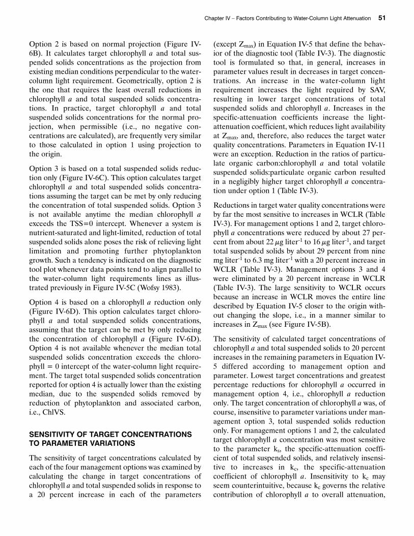
Option 2 is based on normal projection (Figure IV-6B). It calculates target chlorophyll a and total sus-pended solids concentrations as the projection fromexisting median conditions perpendicular to the water-column light requirement. Geometrically, option 2 isthe one that requires the least overall reductions inchlorophyll a and total suspended solids concentra-tions. In practice, target chlorophyll a and totalsuspended solids concentrations for the normal pro-jection, when permissible (i.e., no negative con-centrations are calculated), are frequently very similarto those calculated in option 1 using projection to the origin.

Option 3 is based on a total suspended solids reduc-tion only (Figure IV-6C). This option calculates targetchlorophyll a and total suspended solids concentra-tions assuming the target can be met by only reducingthe concentration of total suspended solids. Option 3is not available anytime the median chlorophyll aexceeds the TSS=0 intercept. Whenever a system isnutrient-saturated and light-limited, reduction of totalsuspended solids alone poses the risk of relieving lightlimitation and promoting further phytoplanktongrowth. Such a tendency is indicated on the diagnostictool plot whenever data points tend to align parallel tothe water-column light requirements lines as illus-trated previously in Figure IV-5C (Wofsy 1983).

Option 4 is based on a chlorophyll a reduction only(Figure IV-6D). This option calculates target chloro-phyll a and total suspended solids concentrations,assuming that the target can be met by only reducingthe concentration of chlorophyll a (Figure IV-6D).Option 4 is not available whenever the median totalsuspended solids concentration exceeds the chloro-phyll = 0 intercept of the water-column light require-ment. The target total suspended solids concentrationreported for option 4 is actually lower than the existingmedian, due to the suspended solids removed byreduction of phytoplankton and associated carbon,i.e., ChlVS.

SENSITIVITY OF TARGET CONCENTRATIONSTO PARAMETER VARIATIONS

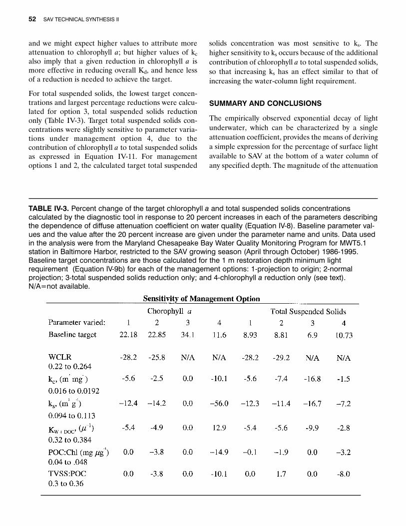
The sensitivity of target concentrations calculated byeach of the four management options was examined bycalculating the change in target concentrations ofchlorophyll a and total suspended solids in response toa 20 percent increase in each of the parameters

(except Zmax) in Equation IV-5 that define the behav-ior of the diagnostic tool (Table IV-3). The diagnostictool is formulated so that, in general, increases inparameter values result in decreases in target concen-trations. An increase in the water-column lightrequirement increases the light required by SAV,resulting in lower target concentrations of totalsuspended solids and chlorophyll a. Increases in thespecific-attenuation coefficients increase the light-attenuation coefficient, which reduces light availabilityat Zmax, and, therefore, also reduces the target waterquality concentrations. Parameters in Equation IV-11were an exception. Reduction in the ratios of particu-late organic carbon:chlorophyll a and total volatilesuspended solids:particulate organic carbon resultedin a negligibly higher target chlorophyll a concentra-tion under option 1 (Table IV-3).

Reductions in target water quality concentrations wereby far the most sensitive to increases in WCLR (TableIV-3). For management options 1 and 2, target chloro-phyll a concentrations were reduced by about 27 per-cent from about 22 µg liter-1 to 16 µg liter-1, and targettotal suspended solids by about 29 percent from ninemg liter-1 to 6.3 mg liter-1 with a 20 percent increase inWCLR (Table IV-3). Management options 3 and 4were eliminated by a 20 percent increase in WCLR(Table IV-3). The large sensitivity to WCLR occursbecause an increase in WCLR moves the entire linedescribed by Equation IV-5 closer to the origin with-out changing the slope, i.e., in a manner similar toincreases in Zmax (see Figure IV-5B).

The sensitivity of calculated target concentrations ofchlorophyll a and total suspended solids to 20 percentincreases in the remaining parameters in Equation IV-5 differed according to management option andparameter. Lowest target concentrations and greatestpercentage reductions for chlorophyll a occurred inmanagement option 4, i.e., chlorophyll a reductiononly. The target concentration of chlorophyll a was, ofcourse, insensitive to parameter variations under man-agement option 3, total suspended solids reductiononly. For management options 1 and 2, the calculatedtarget chlorophyll a concentration was most sensitiveto the parameter ks, the specific-attenuation coeffi-cient of total suspended solids, and relatively insensi-tive to increases in kc, the specific-attenuationcoefficient of chlorophyll a. Insensitivity to kc mayseem counterintuitive, because kc governs the relativecontribution of chlorophyll a to overall attenuation,


and we might expect higher values to attribute moreattenuation to chlorophyll a; but higher values of kc

also imply that a given reduction in chlorophyll a ismore effective in reducing overall Kd, and hence lessof a reduction is needed to achieve the target.

For total suspended solids, the lowest target concen-trations and largest percentage reductions were calcu-lated for option 3, total suspended solids reductiononly (Table IV-3). Target total suspended solids con-centrations were slightly sensitive to parameter varia-tions under management option 4, due to thecontribution of chlorophyll a to total suspended solidsas expressed in Equation IV-11. For managementoptions 1 and 2, the calculated target total suspended

solids concentration was most sensitive to ks. Thehigher sensitivity to ks occurs because of the additionalcontribution of chlorophyll a to total suspended solids,so that increasing ks has an effect similar to that ofincreasing the water-column light requirement.

SUMMARY AND CONCLUSIONS

The empirically observed exponential decay of lightunderwater, which can be characterized by a singleattenuation coefficient, provides the means of derivinga simple expression for the percentage of surface lightavailable to SAV at the bottom of a water column ofany specified depth. The magnitude of the attenuation


TABLE IV-3. Percent change of the target chlorophyll a and total suspended solids concentrationscalculated by the diagnostic tool in response to 20 percent increases in each of the parameters describingthe dependence of diffuse attenuation coefficient on water quality (Equation IV-8). Baseline parameter val-ues and the value after the 20 percent increase are given under the parameter name and units. Data usedin the analysis were from the Maryland Chesapeake Bay Water Quality Monitoring Program for MWT5.1station in Baltimore Harbor, restricted to the SAV growing season (April through October) 1986-1995.Baseline target concentrations are those calculated for the 1 m restoration depth minimum lightrequirement (Equation IV-9b) for each of the management options: 1-projection to origin; 2-normalprojection; 3-total suspended solids reduction only; and 4-chlorophyll a reduction only (see text). N/A=not available.

coefficient is governed mainly by the concentrations ofthree water quality parameters: dissolved organic car-bon, chlorophyll a and total suspended solids. Ofthese, only chlorophyll a and total suspended solidsshow substantial contribution to light attenuation atmost locations around Chesapeake Bay. Sites wherecolored dissolved organic matter contributes substan-tially to attenuation, such as the Pocomoke River onthe Maryland/Virginia border, are not considered inthis analysis.

Linear partitioning of the diffuse-attenuation coeffi-cient into contributions due to water plus dissolvedorganic carbon, phytoplankton chlorophyll a and totalsuspended solids involves known compromises in real-ism but is an approximation that has proved useful inthe past and leads to a tractable solution for purposesof water quality management. Due to unexplainedvariability in the data from the Chesapeake Bay WaterQuality Monitoring Program, specific-attenuationcoefficients for water plus dissolved organic carbon,chlorophyll a and total suspended solids were esti-mated by a combined approach using statisticalregression, optical modeling and comparison withliterature values.

It will be shown elsewhere (Gallegos, unpublished) thatthe use of a single linear regression (Equation IV- 4),when applied across the full range of observed water quality conditions, produces biased diffuse-attenuation coefficients with respect to a more mecha-nistic model of light attenuation. Nevertheless,unbiased diffuse-attenuation coefficients can beobtained from a suitably calibrated optical waterquality model. The present version of the diagnostictool incorporates unbiased diffuse-attenuation coeffi-cients determined by an optical model calibrated for asite near the mesohaline region of the mainstem Bay(Gallegos 1994). There is an urgent need for a region-ally customized application of this approach (see“Directions for Future Research”).

The diagnostic tool is based on a plot of measuredconcentrations of total suspended solids versus chloro-phyll a, in relation to the linear combination of totalsuspended solids and chlorophyll a that meet the min-imum light habitat requirement. Characteristic behav-iors can be identified by the orientation of points:points scattered along the vertical (TSS) axis indicateattenuation dominated by episodic inputs of total sus-pended solids; points oriented parallel to the line

defining the contribution of chlorophyll a to total sus-pended solids indicate variation of light attenuationgoverned by phytoplankton blooms; and points ori-ented parallel to the line describing the water-columnlight habitat requirement indicate that maximalchlorophyll concentrations are dependent on theconcentration of total suspended solids, signifying anutrient-saturated system.

An analysis of total suspended solids indicated thattotal volatile suspended solids were a variable fractionof total suspended solids, and that on average, partic-ulate organic carbon is about 30 percent of totalvolatile suspended solids. Using a reasonable estimateof the phytoplankton carbon:chlorophyll a ratio, alongwith the contribution of particulate organic carbon tototal volatile suspended solids, indicated that phyto-plankton carbon contributes to the overall total sus-pended solids. Any reduction in chlorophyll a wouldbe accompanied by a proportionate decrease in totalsuspended solids.

Up to four management options for moving the systemto conditions that meet specified water-column lightrequirements are calculated by the diagnostic tool.The precision of the calculations obviously implies adegree of control over water quality conditions thatclearly is not always attainable. Nevertheless, report-ing of four potential targets provides managers with anoverall view of the magnitude of the necessary reduc-tions, and some of the tradeoffs that are available. Fur-thermore, the spreadsheet reports the frequency withwhich the water-column light requirements for eachrestoration depth are violated by the individual meas-urements. This information may be useful in the futureif water-column light requirements for SAV growthand survival become better understood in terms oftolerance of short-term light reductions.

Directions for Future Research

Continued collection of monitoring data is necessaryto track recovery (or further degradation) of the sys-tem with respect to the optical water quality targetsdefined for the various regions using the diagnostictool. However, it is doubtful that additional monitor-ing data will improve the ability to derive statisticalestimates of specific-attenuation coefficients byregression analysis. Inherent variability in the spectralabsorption and scattering properties of the opticalwater quality parameters, combined with normal


uncertainty associated with sampling and laboratoryanalyses, probably account for the low coefficients ofdetermination and statistically insignificant estimatesof some specific-attenuation coefficients.

Nevertheless, some attempt to determine regionallybased estimates of optical properties should be made,

because of the pronounced changes in the nature ofparticulate material that occur from the headwaters tothe mouth of major tributaries as well as the mainstemChesapeake Bay itself. An approach based on directmeasurement of particulate absorption spectra andoptical modeling will be needed to obtain regionallycustomized diagnostic tools.


chapter iv factors contributing to water-column light

Documents