chapter 2pongsak.ee.engr.tu.ac.th/le426/doc/optcommc2.pdf · in this chapter we deal with optical...

Chapter 2

Optical Fibers: Structures,

Waveguiding & Fabrication

Outline

• Review of Maxwell’s Equations and Plane waves

• Nature of Light

• Parallel Slab Waveguide

• Optical Fiber

• Optical Fiber Material and Fabrication

Theories of Optics

• Light is an electromagentic phenomenon described by the same

theoretical principles that govern all forms of electromagnetic

radiation. Maxwell’s equations are in the hurt of electromagnetic

theory & is fully successful in providing treatment of light

propagation. Electromagnetic optics provides the most complete

treatment of light phenomena in the context of classical optics.

• Turning to phenomena involving the interaction of light & matter,

such as emission & absorption of light, quantum theory provides

the successful explanation for light-matter interaction. These

phenomena are described by quantum electrodynamics which is the

marriage of electromagnetic theory with quantum theory. For optical

phenomena, this theory also referred to as quantum optics. This

theory provides an explanation of virtually all optical phenomena.

• In the context of classical optics, electromagentic radiation propagates

in the form of two mutually coupled vector waves, an electric field-

wave & magnetic field wave. It is possible to describe many optical

phenomena such as diffraction, by scalar wave theory in which light is

described by a single scalar wavefunction. This approximate theory is

called scalar wave optics or simply wave optics. When light propagates

through & around objects whose dimensions are much greater than the

optical wavelength, the wave nature of light is not readily discerned, so

that its behavior can be adequately described by rays obeying a set of

geometrical rules. This theory is called ray optics. Ray optics is the

limit of wave optics when the wavelength is very short.

Quantum Optics

Electromagnetic Optics

Wave Optics

Ray Optics

Engineering Model

• In engineering discipline, we should choose the appropriate &

easiest physical theory that can handle our problems.

Therefore, specially in this course we will use different optical

theories to describe & analyze our problems. In this chapter we

deal with optical transmission through fibers, and other optical

waveguiding structures. Depending on the structure, we may

use ray optics or electromagnetic optics, so we begin our

discussion with a brief introduction to electromagnetic optics,

ray optics & their fundamental connection, then having

equipped with basic theories, we analyze the propagation of

light in the optical fiber structures.

Electromagnetic Optics

• Electromagnetic radiation propagates in the form of two mutually coupled

vector waves, an electric field wave & a magnetic field wave. Both are

vector functions of position & time.

• In a source-free, linear, homogeneous, isotropic & non-dispersive media,

such as free space, these electric & magnetic fields satisfy the following

partial differential equations, known as Maxwell’ equations:

0

0

=⋅∇

=⋅∇

∂∂

−=×∇

∂∂

=×∇

H

E

t

HE

t

EH

r

r

rr

rr

µ

ε

• In Maxwell’s equations, E is the electric field expressed in [V/m], H is the

magnetic field expressed in [A/m].

• The solution of Maxwell’s equations in free space, through the wave

equation, can be easily obtained for monochromatic electromagnetic

wave. All electric & magnetic fields are harmonic functions of time of the

same frequency. Electric & magnetic fields are perpendicular to each other

& both perpendicular to the direction of propagation, k, known as

transverse wave (TEM). E, H & k form a set of orthogonal vectors.

ty permeabili Magnetic :[H/m]

ty permittivi Electric :[F/m]

µε

operation curl is :

operation divergence is :

∇×

⋅∇

Electromagnetic Plane wave in Free space

Ex

z

Direction of Propagation

By

z

x

y

k

An electromagnetic wave is a travelling wave which has timevarying electric and magnetic fields which are perpendicular to eachother and the direction of propagation, z.

S.O.Kasap, optoelectronics and Photonics Principles and Practices, prentice hall, 2001

Linearly Polarized Electromagnetic Plane wave

:[m/s] 1

: ][

:2

:

: 2ω

:where

)ωcos(e

)-ωcos(e

0

0

0

0

µε

εµ

η

πλ

π

=

Ω==

=

=

−=

=

v

H

E

k

k

f

kztHH

kztEE

y

x

yy

xxr

r

Angular frequency [rad/m]

Wavenumber or wave propagation constant [1/m]

Wavelength [m]

intrinsic (wave) impedance

velocity of wave propagation

z

Ex

= Eosin(ωt–kz)

Ex

z

Propagation

E

H

k

E and H have constant phase

in this xy plane; a wavefront

E

A plane EM wave travelling along z, has the same Ex (or By) at any point in a

given xy plane. All electric field vectors in a given xy plane are therefore in phase.The xy planes are of infinite extent in the x and y directions.


Some Wave Parameters

• Wavelength is the distance over which the phase changes by 2π .

• In vacuum (free space):

• Refractive index of a medium is defined as:

• For non-magnetic media (µr = 1) :

f

v=λ

][ 120 m/s 103

[H/m] 104 [F/m] 36

10

0

8

7

0

9

0

Ω=×≅=

×== −−

πη

µπ

ε

cv

:

:

mediumin wave)(EMlight ofvelocity

in vacuum wave)(EMlight ofvelocity

00

r

r

rrv

cn

ε

µ

εµεµ

µε====

Relative magnetic permeability

Relative electric permittivity

rn ε=

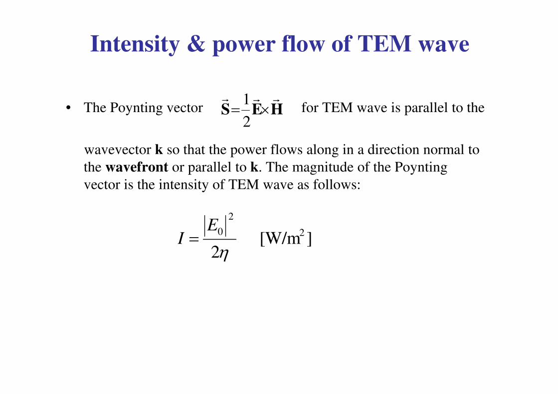
Intensity & power flow of TEM wave

• The Poynting vector for TEM wave is parallel to the

wavevector k so that the power flows along in a direction normal to

the wavefront or parallel to k. The magnitude of the Poynting

vector is the intensity of TEM wave as follows:

HESrrr

×=2

1

][W/m 2

2

2

0

η

EI =

Connection between EM wave optics &

Ray optics

According to wave or physical optics viewpoint, the EM waves radiated by

a small optical source can be represented by a train of spherical wavefronts

with the source at the center. A wavefront is defined as the locus of all

points in the wave train which exhibit the same phase. Far from source

wavefronts tend to be in a plane form. Next page you will see different

possible phase fronts for EM waves.

When the wavelength of light is much smaller than the object, the

wavefronts appear as straight lines to this object. In this case the light wave

can be indicated by a light ray, which is drawn perpendicular to the phase

front and parallel to the Poynting vector, which indicates the flow of

energy. Thus, large scale optical effects such as reflection & refraction can

be analyzed by simple geometrical process called ray tracing. This view of

optics is referred to as ray optics or geometrical optics (GO).

k

Wave fronts

r

E

k

Wave fronts(constant phase surfaces)

z

λλλλλλλλ

λλλλ

Wave fronts

PO

P

A perfect spherical waveA perfect plane wave A divergent beam

(a) (b) (c)

Examples of possible EM waves


rays

General form of linearly polarized plane waves

)(tan

OR0;

)ωcos(ˆ)ωcos(ˆ

0

01

2

0

2

0

00

x

y

yx

yyxx

E

E

EEEE

kztEkztEE

−=

=+==

+−+−=

θ

πδ

δr

ree

Any two orthogonal plane waves

Can be combined into a linearly

Polarized wave. Conversely, any

arbitrary linearly polarized wave

can be resolved into two

independent Orthogonal plane

waves that are in phase.

Optical Fiber communications, 3rd ed.,G.Keiser,McGrawHill, 2000

Elliptically Polarized plane waves

2

0

2

0

00

2

00

2

0

2

0

0

cos2)2tan(

sincos2

)ωcos(e)ωcos(e

Eee

yx

yx

y

y

x

x

y

y

x

x

yxx

yyxx

EE

EE

E

E

E

E

E

E

E

E

kztkztE

EE

−=

=

−

+

+−+−=

+=

δα

δδ

δ

r

[2-16]


Circularly polarized waves

2 & :onpolarizatiCircular 000

πδ ±=== EEE yx


+ Sign : Clockwise of Right Circularly

Polarized (RCP)

- Sign : Counterclockwise of Left

Circularly Polarized (LCP)

Laws of Reflection & Refraction

Reflection law: angle of incidence=angle of reflection

Snell’s law of refraction:

2211 sinsin φφ nn =Optical Fiber communications, 3rd ed.,G.Keiser,McGrawHill, 2000

Total internal reflection, Critical angle

1

2sinn

nc =φ

1θ

n2

n1

> n2

Incident

light

Transmitted

(refracted) light

Reflected

light

kt

TIR

Evanescent wave

ki

kr

(a) (b) (c)

Light wave travelling in a more dense medium strikes a less dense medium. Depending onthe incidence angle with respect to , which is determined by the ratio of the refractive

indices, the wave may be transmitted (refracted) or reflected. (a) (b) (c)

and total internal reflection (TIR).

2φ

1φ cφ

o902 =φ

cφφ >1

cφ

cφφ <1 cφφ =1

cφφ >1

Critical angle

1

2sinn

nc =φ

Phase shift due to TIR

• The totally reflected wave experiences a phase shift however

which is given by:

• Where (p,N) refer to the electric field components parallel

(Parallel Polarization, TM) or normal (Perpendicular

Polarization, TE) to the plane of incidence respectively.

2

1

1

1

22

1

1

22

sin

1cos

2 tan;

sin

1cos

2tan

n

nn

nn

n

n pN

=

−−=

−−=

θθδ

θθδ

2.19a-b

Optical waveguiding by TIR:

Dielectric Slab Waveguide

Propagation mechanism in an ideal step-index optical waveguide.


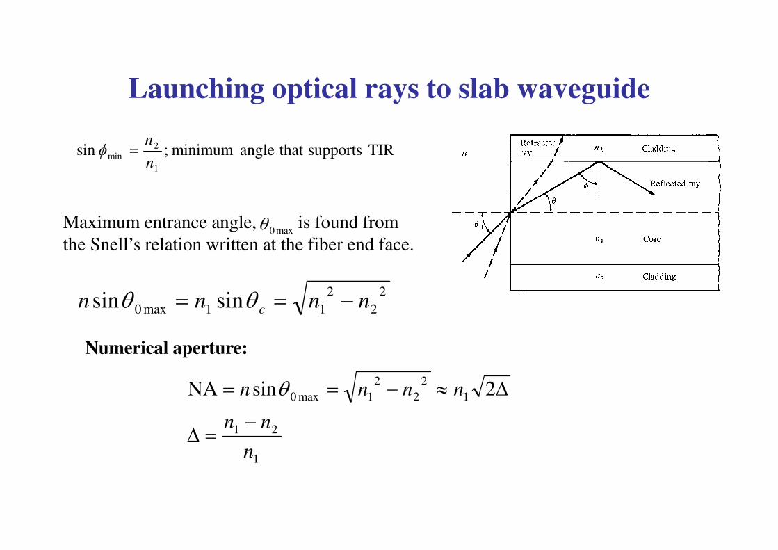
TIR supports that angle minimum ;sin1

2min

n

n=φ

2

2

2

11max0 sinsin nnnn c −== θθ

Maximum entrance angle, is found from

the Snell’s relation written at the fiber end face.max0θ

Launching optical rays to slab waveguide

Numerical aperture:

1

21

1

2

2

2

1max0 2sinNA

n

nn

nnnn

−=∆

∆≈−== θ

Optical rays transmission through dielectric

slab waveguide

ccnn φπ

θθ −=<>2

;21

−=

−

θ

θπλ

θπsin

cos

2

sintan

1

2

2

22

11

n

nnmdn

For TE-case, when electric waves are normal to the plane of incidencemust be satisfied with following relationship:θ


O

EM analysis of Slab waveguide

• For each particular angle, in which light ray can be faithfully transmitted

along slab waveguide, we can obtain one possible propagating wave

solution from a Maxwell’s equations or mode.

• The modes with electric field perpendicular to the plane of incidence (page)

are called TE (Transverse Electric) and numbered as:

Electric field distribution of these modes for 2D slab waveguide can be

expressed as:

wave transmission along slab waveguides, fibers & other type of optical

waveguides can be fully described by time & z dependency of the mode:

,...TE,TE,TE 210

number) (mode 3,2,1,0

)ωcos()(e),,,(

=

−=

m

ztyftzyxE mmxm βr

)(or )ωcos(

ztj

mmezt

βωβ −−

TE modes in slab waveguide

z

y

number) (mode 3,2,1,0

)ωcos()(e),,,(

=

−=

m

ztyftzyxE mmxm βr


Modes in slab waveguide

• The order of the mode is equal to the # of field zeros across the guide. The

order of the mode is also related to the angle in which the ray congruence

corresponding to this mode makes with the plane of the waveguide (or axis

of the fiber). The steeper the angle, the higher the order of the mode.

• For higher order modes the fields are distributed more toward the edges of

the guide and penetrate further into the cladding region.

• Radiation modes in fibers are not trapped in the core & guided by the fiber

but they are still solutions of the Maxwell’ eqs. with the same boundary

conditions. These infinite continuum of the modes results from the optical

power that is outside the fiber acceptance angle being refracted out of the

core.

• In addition to bound & refracted (radiation) modes, there are leaky modes

in optical fiber. They are partially confined to the core & attenuated by

continuously radiating this power out of the core as they traverse along the

fiber (results from Tunneling effect which is quantum mechanical

phenomenon.) A mode remains guided as long as knkn 12 << β

Example

Basic structure of all optical fiber

• Core—carries most of light

• Cladding—confines light to core

• In some fibers, substrate glass layer to add strength

• Inner jacket or primary buffer coating—mechanical

protection

• Outer jacket or secondary buffer coating—

mechanical protection

Source: Optical Cable Corporation

Three Types of Optical Fibers


Optical fiber standard dimensions

• Core, cladding, jacketing standardized

• Jacket: 245 µm

Source: Corning

Modal Theory of Step Index fiber

• General expression of EM-wave in the circular fiber can be written as:

• Each of the characteristic solutions is

called mth mode of the optical fiber.

• It is often sufficient to give the E-field of the mode.

∑∑

∑∑−

−

==

==

m

ztj

mm

m

mm

m

ztj

mm

m

mm

m

m

erVAtzrHAtzrH

erUAtzrEAtzrE

)ω(

)ω(

),(),,,(),,,(

),(),,,(),,,(

β

β

φφφ

φφφ

rrr

rrr

),,,( & ),,,( tzrHtzrE mm φφrr

1,2,3...m ),()ω( =− ztj

mmerU

βφr

• The modal field distribution, , and the mode

propagation constant, are obtained from solving the

Maxwell’s equations subject to the boundary conditions given

by the cross sectional dimensions and the dielectric constants

of the fiber.

• Most important characteristics of the EM transmission along the fiber are

determined by the mode propagation constant, , which depends on

the mode & in general varies with frequency or wavelength. This quantity

is always between the plane propagation constant (wave number) of the

core & the cladding media .

),( φrUm

r

mβ

)ω(mβ

knkn m 12 )ω( << β

• At each frequency or wavelength, there exists only a finite number

of guided or propagating modes that can carry light energy over a

long distance along the fiber. Each of these modes can propagate in

the fiber only if the frequency is above the cut-off frequency, ωc

, (or the source wavelength is shorter than the cut-off wavelength)

obtained from cut-off condition that is:

• To minimize the signal distortion, the fiber is often operated in a

single mode regime. In this regime only the lowest order mode

(fundamental mode) can propagate in the fiber and all higher order

modes are under cut-off condition (non-propagating).

• Multi-mode fibers are also extensively used for many applications.

In these fibers many modes carry the optical signal collectively &

simultaneously.

kncm 2)ω( =β

Optical Fiber Modes

• The optical fiber has a circular waveguide instead of planar

• The solutions to Maxwell’s equations

– Fields in core are non-decaying

• J, Y Bessel functions of first and second kind

– Fields in cladding are decaying

• K modified Bessel functions of second kind

• Solutions vary with radius r and angle θ

• There are two mode number to specify the mode

– m is the radial mode number

– ν is the angular mode number

Bessel Functions

Bessel Function Relationships• Bessel function recursive relationships

• Small argument approximations

( ) ( ) ( )xJxJ n

n

n 1−=−

( ) ( )xKxK nn =−

( ) ( ) ( )xJxJx

nxJ nnn 11

2+− −=

( ) ( ) ( )xJxJx

xJ 210

2−=

( ) ( ) ( )xKxKx

nxK nnn 11

2+− +−=

( ) ( ) ( )xKxKx

xK 210

2+−=

( )( )

>

−

=−

−→

02

2

!1

00.57722

ln

nx

n

nx

xK nn

Mode designation in circular cylindrical

waveguide (Optical Fiber)

:modesEH Hybrid

:modesHE Hybrid

:modesTM

:modes TE

m

m

m

m

ν

ν

ν

ν The electric field vector lies in transverse plane.

The magnetic field vector lies in transverse plane.

Ez component is larger than Hz component.

Hz component is larger than Ez component.

ν= # of variation cycles or zeros in φ direction.

m= # of variation cycles or zeros in r direction.

x

y

r

z

φ

Example of TE Modes

Given n1 = 1.5, n2 = 1.45, a = 5 µm. λ = 1.3 µm. Find

TE modes. The characteristic equation is given by:

Characteristic equation plot

0)(

)(

)(

)(

0

1

0

1 =+wawK

waK

uauJ

uaJ

)(/)( 01 wawKwaK−

)(/)( 01 uauJuaJ

u

Ray Optics Theory (Step-Index Fiber)

Skew rays

When ν=0 (no φ-variation), rays lie in a plane that intersects the fiber

axis, which is called “meridional” rays. Hybrid modes has φ-variation,

resulting in “skew” rays.


Characteristic Equation• Under the weakly guiding approximation (n1-n2)<<1

– Valid for standard telecommunications fibers

• Substitute to eliminate the derivatives

( )( )

( )( )awK

awKwa

auJ

auJua

''

ν

ν

ν

ν =

222

1

22

1

2 ββ −=−= oknku22

2

22

2

22

oknkw −=−= ββ

( ) ( ) ( )x

xJlxJxJ l

ll m1

'

±±= ( ) ( ) ( )x

xKlxKxK l

ll m1

'

±−=

( )( )

( )( )

( )( )

( )( )awK

awKaw

auJ

auJuaor

awK

awKaw

auJ

auJua

ν

ν

ν

ν

ν

ν

ν

ν 1111 ++−− =−=

HE Modes EH Modes

Lowest Order Modes• Look at the ν=-1, 0, 1 modes

• Use Bessel function properties to get positive order and

highest order on top

ν =-1

ν =0

( )( )

( )( )yK

yKy

xJ

xJx

1

2

1

2

−

−

−

− −=

( )( )

( )( )yK

yKy

xJ

xJx

1

2

1

2 =

( )( )

( )( )yK

yKy

xJ

xJx

1

0

1

0 −=

( )( )

( )( )yK

yKy

xJ

xJx

0

1

0

1 −− −=( )( )

( )( )yK

yKy

xJ

xJx

0

1

0

1 =

( )( )

( )( )yK

yKy

xJ

xJx

0

1

0

1 =

uax = awy = 2

2

2

1

22 2nnayxV −=+=

λπ

Lowest Order Modes cont. ν =+1

• So the 6 equations collapse down to 2 equations

( )( )

( )( )yK

yKy

xJ

xJx

1

0

1

0 −=

( )( )

( )( )yK

yKy

xJ

xJx

1

2

1

2 =

( )( )

( )( )yK

yKy

xJ

xJx

1

2

1

2 =

( )( )

( )( )yK

yKy

xJ

xJx

1

2

1

2 =( )( )

( )( )yK

yKy

xJ

xJx

0

1

0

1 =

lowest modes

First Mode Cut-Off• First mode

– What is the smallest allowable V?

– Let y 0 and the corresponding x V

– So V=0, no cut-off for lowest order mode

– Same as a symmetric slab waveguide

( )( )

( )( )

0

5772.02

ln

2

2

1

limlim0

0

1

00

1 =−

−

==→→ y

yy

yK

yKy

VJ

VJV

yy

( ) 01 =VJ

Second Mode Cut-Off• Second mode

( ) ( )VJV

VJ 12

2=

( )( )

( )( )

22

2

1

2

2

1

limlim

2

01

2

01

2 =

==→→

y

yy

yK

yKy

VJ

VJV

yy

( ) ( ) ( )xJxJx

nxJ nnn 11

2−+ −=

( ) ( ) ( )xJxJx

xJ 012

2−=

( ) ( ) ( )VJV

VJVJV

o 11

22=−

( ) 0=VJo

405.2=V

Cut-off Condition

Number of Modes

• The number of modes can be characterized by the normalized frequency

• Most standard optical fibers are characterized by their numerical aperture

• Normalized frequency is related to numerical aperture

• The optical fiber is single mode if V<2.405

• For large normalized frequency the number of modes is approximately

2

2

2

1

2nnaV −=

λπ

2

2

2

1NA nn −=

AaV N2

λπ

=

14

Modes# 2

2>>≈ VV

π

Fiber Modes

Electric Field Profiles

Weakly Guided Modes

• The refractive index difference between the core and

cladding is very small, i.e.,

• There is degeneracy between modes

– Groups of modes travel with the same velocity (βequal)

• Modes are approximated with nearly linearly

polarized modes called LP modes

– LP01 from HE11 (Fundamental Mode)

– LP0m from HE1m

– LP1m sum of TE0m, TM0m, and HE2m

– LPνm sum of HEν+1,m and EHν-1,m

121 <<− nn

Lower-order LP modes

Plot of b-V

Cut-off V-parameter for low-

order LPlm modes

m=1 m=2 m=3

l=0 0 3.832 7.016

l=1 2.405 5.520 8.654

Transverse Electric Field of LP11 mode

LP11 mode

Fundamental Mode (HE11) Field Distribution


Polarizations of fundamental modeMode field diameter (MFD)

Single mode Operation

• The cut-off wavelength or frequency for each mode is obtained from:

• Single mode operation is possible (Single mode fiber) when:

2

)ω( 2c22

c

nnkn

c

clm

ωλπ

β ===

405.2≤V

fiber optical along faithfully propagatecan HEOnly 11

Single-Mode Fibers

• Example: A fiber with a radius of 4 micrometer and

has a normalized frequency of V=2.38 at a wavelength 1 micrometer. The

fiber is single-mode for all wavelengths greater and equal to 1 micrometer.

MFD (Mode Field Diameter): The electric field of the first fundamental

mode can be written as:

min or frequency max @ 2.4 to2.3V

; m 12 to6 ; 1% to%1.0

λµ

=

==∆ a

498.1 & 500.1 21 == nn

);exp()(2

0

2

0W

rErE −=

2/1

0

2

0

32

0

)(

)(222MFD

==

∫∫∞

∞

rdrrE

drrrEW

Birefringence in single-mode fibers

• Because of asymmetries the refractive indices for the two

degenerate modes (vertical & horizontal polarizations) are

different. This difference is referred to as birefringence, :fB

xyf nnB −=


Fiber Beat Length

• In general, a linearly polarized mode is a combination of both

of the degenerate modes. As the modal wave travels along the

fiber, the difference in the refractive indices would change the

phase difference between these two components & thereby the

state of the polarization of the mode. However after certain

length referred to as fiber beat length, the modal wave will

produce its original state of polarization. This length is simply

given by:

f

pkB

Lπ2

=

Multi-Mode Operation

• Total number of modes, M, supported by a multi-mode fiber is

approximately (When V is large) given by:

• Power distribution in the core & the cladding: Another quantity of

interest is the ratio of the mode power in the cladding, to the total

optical power in the fiber, P, which at the wavelengths (or frequencies) far

from the cut-off is given by:

2

4 2

2

2VV

M ≈=π

cladP

MP

Pclad

3

4≈

Power Flow

Intensity Profiles

• Most common single mode optical fiber:

SMF28 from Corning

– Core diameter dcore=8.2 µm

– Outer cladding diameter: dclad=125µm

– Step index

– Numerical Aperture NA=0.14

• NA=sin(θ)

• ∆θ=8°

• λcutoff = 1260nm (single mode for λ>λcutoff)

• Single mode for both λ=1300nm and λ=1550nm

standard telecommunications wavelengths

Standard Single Mode Optical

Fibers

Standard Multimode Optical Fibers

• Most common multimode optical fiber:

62.5/125 from Corning

– Core diameter dcore= 62.5 µm

– Outer cladding diameter: dclad=125µm

– Graded index

– Numerical Aperture NA=0.275

• NA=sin(θ)

• ∆θ=16°

• Many modes

Fiber Materials• Two major types: Glass optical fiber and

Plastic (or Polymer) optical fiber (POF)

• Glass fiber features:

– Advantages: low attenuation, cheap and abundant

raw material (mostly sand)

– Disadvantages: high installation cost, complexity,

requires skilled technicians, inflexible, easy-to-

break

Glass Materials

• Oxide glass

– Silica (SiO2) is most

common; good over wide

range, especially around 1.5

µm

– Use dopants to change

refractive index.

• Metal Halide (Metal+Halogen)

– Fluoride glass : very low loss for mid-infrared (2-5 µm)

range)

• Active glass, like active electronic devices : can be used to

amplify or attenuate; erbium and neodymium are most common.

Plastic Optical Fiber

• Advantages:

– Simpler and less expensive components

– Lighter weight

– greater flexibility and ease in handling and

connecting (POF diameters are 1 mm compared

with 8-100 mm for glass)

– Lower installation cost

• Disadvantages:

– High attenuation

– Limited production

POF Material

• Typically,

– Core : PMMA (poly(methylmethacryclate))

(acrylic), PFP (perfluorinated polymers),

polysterene

– Cladding : Silicone resin, Fluorinated polymer

• Features: High refractive index difference (core

: 1.5-1.6, cladding : 1.46) ; Large NA

• Examples:

– Polysterene core (n=1.6), methy methacrylate

cladding (n=1.49) -> NA = 0.6

Comparison between glass fiber,

POF, copper wire

Types of optical fibers &

Applications

• Single mode glass—long distance

communications

• Multimode glass—short distance

communications

• Plastic—consumer short distance, electronics

& cars

• Hybrid or polymer clad (glass core, plastic

cladding)—lighting, consumer applications

Plastic optical fiber (POF)

• 1000 µm diameter, 980 µm core

• Strong

• Uses LEDs in visible range, 650 nm

• Not suitable for long-distance uses

• Does not transmit infrared

Source: Pofeska/Mitsubishi Rayon Co.

Requirements for fabricating useful

optical fiber• Materials must be extremely pure

– Impurity < 1 part per billion for metals

– Impurity < 1 part per 10 million for water

• About 1000 times more pure than traditional chemical

purification techniques allow

• Dimensions must be controlled to extremely high degree

– Core size, position, cladding size tolerances ~ 1 micron or

less

– Roughly 1 wavelength of light

– Refractive indices must also be very precisely controlled

• Must be made in long lengths

• Must have tensile strength

Fiber Fabrication Procedure

• Direct-melt : like traditional glass-making,

fibers made directly from the molten state of

purified components of silicate glasses

• Vapor phase oxidation : Three Steps are

Involved

– Making a Preform Glass Cylinder

– Drawing of preform down into thin fiber

– Jacketing and cabling

Fiber Fabrication (cont’d)

• First SiO2 particles are formed by reaction of

metal halides vapors and oxygen, then

collected on a bulk glass and sintered ->

preform

• Preform : A solid glass rod or tube which is a

scale model of desired fiber.

• typically around 10 to 25 nm in diameter and

60 to 120 cm long.

Purification of silica :

a two-step process

• First: use distillation

– Heat silica to boiling point (2230o C), condense

gas

– Metals are heavier and do not boil at this

temperature

– Yields impurity levels of ~ 10-6

• Second stage takes place when fiber fabricated

Fiber fabrication process

• Called “Outside Vapor Deposition Process” or

OVD process

• Stages

– Laydown

– Consolidation

– Drawing

First stage: Laydown

• Vapor deposition from ultrapure vapors

• Soot preform made when vapors exposed to

burner and form fine soot particles of silica

and germanium(From particles of silica and germania)

Source: Corning

Outside Vapor Phase Oxidation (OVPO)

Laydown (continued)

• Particles deposited on surface of rotating bait

rod

– Core first

– Then silica cladding

• Vapor deposition process purifies fiber

material as impurities do not deposit as rapidly

• Preform is somewhat porous at this stage

Second stage: consolidation

• Bait rod removed

• Placed in high-temperature consolidation

furnace

– Water vapor removed

– Preform sintered into solid, dense, transparent

glass

• Has same cross-section profile as final fiber,

but is much larger (1-2.5 cm, final: 125 µm =

.0125 cm)

Third stage:

drawing• Done in “draw tower”

• Glass blank from consolidation

stage lowered into draw furnace

• Tip heated until “gob” of glass falls

– Pulls behind it a thin strand of

glass

• Gob cut off

• Strand threaded into computer-

controlled tractor assembly

• Sensors control speed of drawing to

make precise diameter

1850-2000o C

Source: Corning

Fiber Drawing

Drawing (continued)

• Diameter measured hundreds of times per second

– Ensures precise outside dimension

• Primary and secondary coatings (jackets) applied

• At end, fiber wound onto spools for further processing

Gob forming,Source: Corning

Draw tower

Source: Axsys

Other methods used to make fiber

• Vapor phase axial deposition (VAD)

– Batch process

– Preforms can be drawn up to 250 km

– Flame hydrolysis

• Soot formed and deposited by torches

VAD process (continued)

Source: Dutton

Other methods used to make fiber

(continued)• Modified chemical vapor deposition

(MCVD)

– Silica formed inside silica tube in gaseous phase

reaction

– Soot deposited on inside of tube

– Burners traverse tube

• Sinters soot

• Produces highly controllable RI profile

– At end, tube evacuated, sides collapse

MCVD process

Source: Fotec

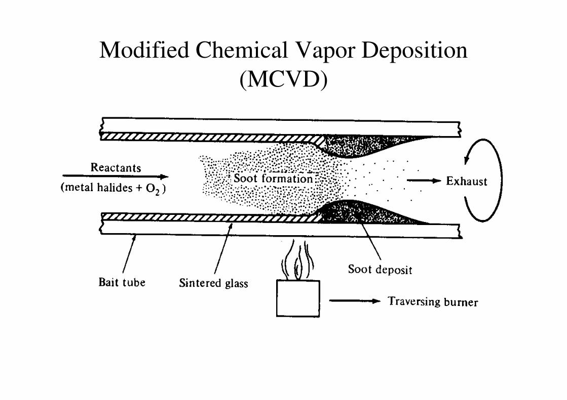
Modified Chemical Vapor Deposition

(MCVD)

Plasma-Activated Chemical Vapor Deposition

(PCVD)

Basic cable construction: types

• Tight buffered

– No room for fibers to move inside of cable

• Loose tube

– Multiple fibers loose inside of outer plastic tube

– Advantage is that with extra length of fiber inside tube due

to curling, less likelihood of damage in sharp bends

• Loose tube with gel filler

– Multiple fibers immersed in gel inside of plastic tube

Source: Dutton

Typical indoor cable

• Single core or double core

– Utilize substrate for additional strength (aramid or

fiberglass)

Source: Dutton

Tight buffered indoor cable

• Application: building risers

• 6 or 12 fibers typically

• Central strength member supports weight of cable

• Tight buffering means that fibers are not put under

tension due to their own weight

Source: Dutton

Outdoor cable

• More rugged, larger number of fibers per cable

– 6 fibers/tube, 6 tubes = 36 fibers

– 8 fibers/tube, 12 tubes = 96 fibers

• Steel or plastic used for strength member

• Outer nylon layer in locations where termites are a

problem

Source: Dutton

Outdoor cable (continued)

Source: Dutton

Submarine cable• Smaller number of fibers because mechanical requirements

much greater

– 4 to 20 typically

• Must withstand high pressure, damage from anchors,

trawlers, etc.

• Cables for shallow water are in greatest danger

– Typically heavily armored

Source: Dutton

Fiber Cross-sections

chapter 2pongsak.ee.engr.tu.ac.th/le426/doc/optcommc2.pdf · in this chapter we deal with optical...

Documents