chapter iii: ranking principles information retrieval & data mining universität des saarlandes,...
TRANSCRIPT

Chapter III:Ranking Principles
Information Retrieval & Data Mining
Universität des Saarlandes, Saarbrücken
Winter Semester 2011/12
IR&DM, WS'11/12
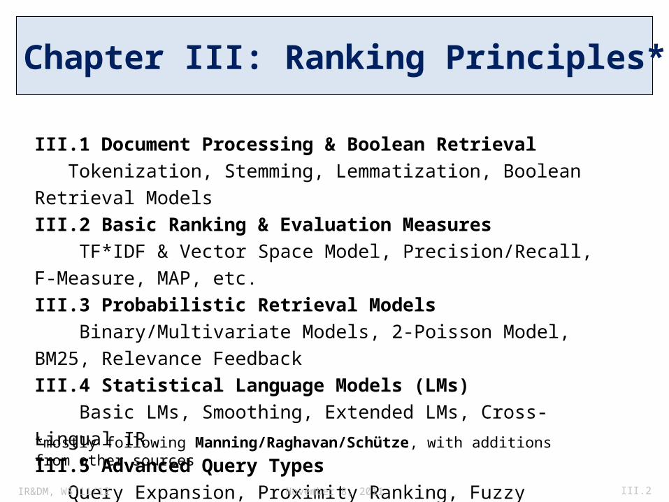
Chapter III: Ranking Principles*
III.1 Document Processing & Boolean Retrieval
Tokenization, Stemming, Lemmatization, Boolean Retrieval Models
III.2 Basic Ranking & Evaluation Measures
TF*IDF & Vector Space Model, Precision/Recall, F-Measure, MAP, etc.
III.3 Probabilistic Retrieval Models
Binary/Multivariate Models, 2-Poisson Model, BM25, Relevance Feedback
III.4 Statistical Language Models (LMs)
Basic LMs, Smoothing, Extended LMs, Cross-Lingual IR
III.5 Advanced Query Types
Query Expansion, Proximity Ranking, Fuzzy Retrieval, XML-IR
*mostly following Manning/Raghavan/Schütze, with additions from other sources
November 8, 2011 III.2
IR&DM, WS'11/12
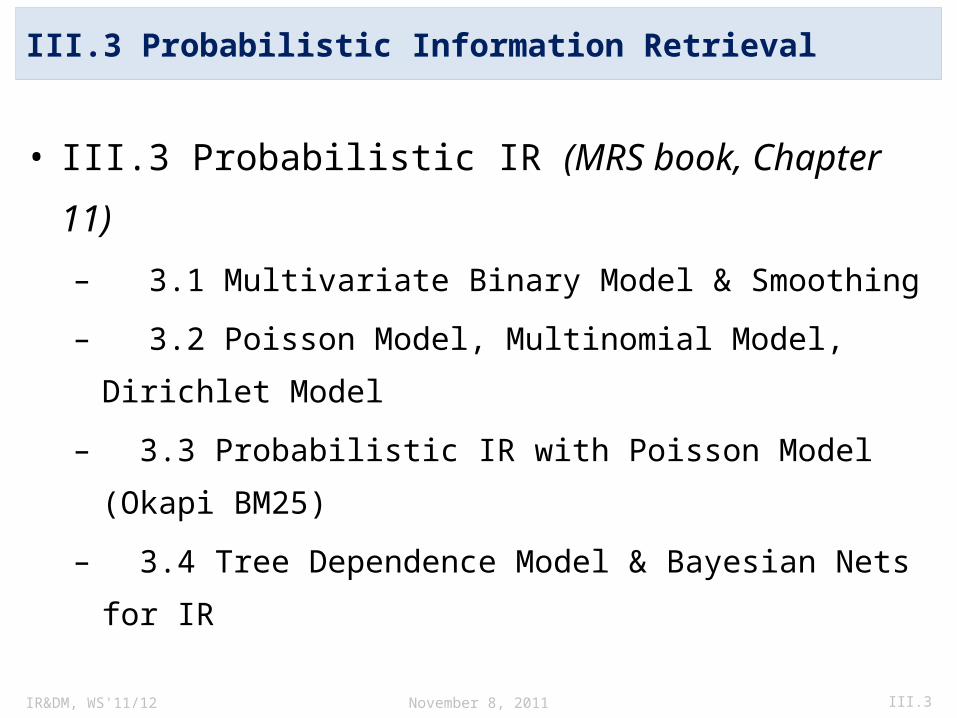
• III.3 Probabilistic IR (MRS book, Chapter 11)
– 3.1 Multivariate Binary Model & Smoothing
– 3.2 Poisson Model, Multinomial Model, Dirichlet Model
– 3.3 Probabilistic IR with Poisson Model (Okapi BM25)
– 3.4 Tree Dependence Model & Bayesian Nets for IR
III.3 Probabilistic Information Retrieval
November 8, 2011 III.3
IR&DM, WS'11/12
TF*IDF vs. Probabilistic Models• TF*IDF sufficiently effective in practice but often criticized for
being “too ad-hoc”• Typically outperformed by probabilistic ranking models and/or
statistical language models in all of the major IR benchmarks: – TREC: http://trec.nist.gov/– CLEF: http://clef2011.org/– INEX: https://inex.mmci.uni-saarland.de/
• Family of Probabilistic IR Models – Generative models for documents as bags-of-words – Binary independence model vs. multinomial (& multivariate) models
• Family of Statistical Language Models– Generative models for documents (and queries) as entire sequences of words– Divergence of document and query distributions (e.g., Kullback-Leibler)
November 8, 2011 III.4

IR&DM, WS'11/12
“Is This Document Relevant? … Probably”
A survey of probabilistic models in information retrieval.
Fabio Crestani, Mounia Lalmas, Cornelis J. Van Rijsbergen, and Iain Campbell
Computer Science Department
University of Glasgow
November 8, 2011 III.5
IR&DM, WS'11/12
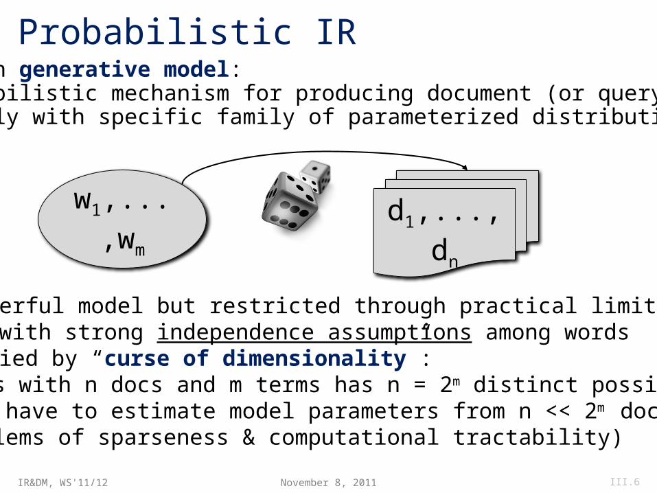
Probabilistic IR
Very powerful model but restricted through practical limitations:• often with strong independence assumptions among words• justified by “curse of dimensionality”:
corpus with n docs and m terms has n = 2m distinct possible docswould have to estimate model parameters from n << 2m docs (problems of sparseness & computational tractability)
Based on generative model: • probabilistic mechanism for producing document (or query)• usually with specific family of parameterized distribution
w1,...,wm d1,...,dn
November 8, 2011 III.6
IR&DM, WS'11/12
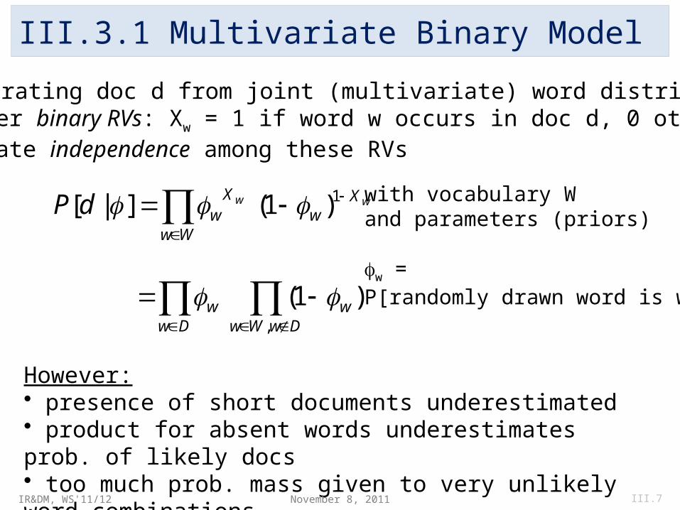
III.3.1 Multivariate Binary ModelFor generating doc d from joint (multivariate) word distribution • consider binary RVs: Xw = 1 if word w occurs in doc d, 0 otherwise• postulate independence among these RVs
ww Xw
Ww
XwdP
1)1(]|[ with vocabulary W
and parameters (priors) w =P[randomly drawn word is w]
Dw DwWw
ww,
)1(
However: • presence of short documents underestimated• product for absent words underestimates prob. of likely docs• too much prob. mass given to very unlikely word combinations
November 8, 2011 III.7
IR&DM, WS'11/12
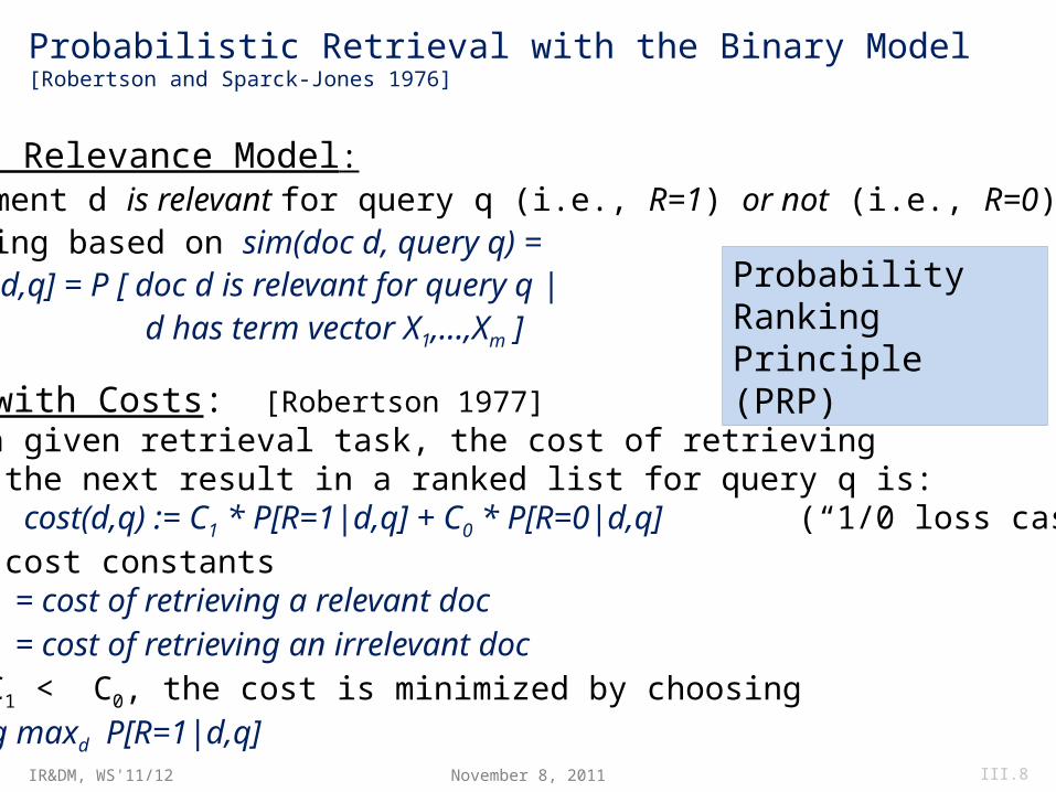
Probabilistic Retrieval with the Binary Model[Robertson and Sparck-Jones 1976]
PRP with Costs: [Robertson 1977]For a given retrieval task, the cost of retrievingd as the next result in a ranked list for query q is: cost(d,q) := C1 * P[R=1|d,q] + C0 * P[R=0|d,q] (“1/0 loss case”)with cost constants
C1 = cost of retrieving a relevant docC0 = cost of retrieving an irrelevant doc
For C1 < C0, the cost is minimized by choosing arg maxd P[R=1|d,q]
Binary Relevance Model: • Document d is relevant for query q (i.e., R=1) or not (i.e., R=0)• Ranking based on sim(doc d, query q) = P[R=1|d,q] = P [ doc d is relevant for query q | d has term vector X1,...,Xm ]
Probability Ranking Principle (PRP)
November 8, 2011 III.8
IR&DM, WS'11/12
Optimality of PRP
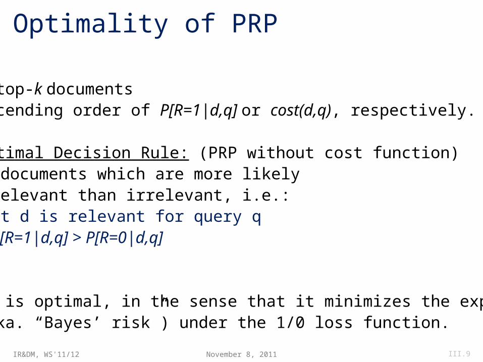
Goal: Return top-k documents in descending order of P[R=1|d,q] or cost(d,q), respectively.
Bayes’ Optimal Decision Rule: (PRP without cost function)Return documents which are more likely to be relevant than irrelevant, i.e.:Document d is relevant for query q iff P[R=1|d,q] > P[R=0|d,q]
Theorem: The PRP is optimal, in the sense that it minimizes the expected loss (aka. “Bayes’ risk”) under the 1/0 loss function.
November 8, 2011 III.9
IR&DM, WS'11/12
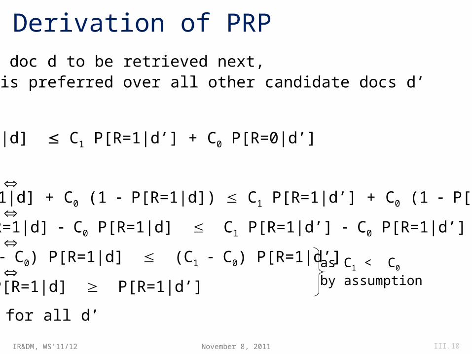
Derivation of PRPConsider doc d to be retrieved next, i.e., d is preferred over all other candidate docs d’
cost(d) :=
C1 P[R=1|d] + C0 P[R=0|d] C1 P[R=1|d’] + C0 P[R=0|d’]
=: cost(d’)
C1 P[R=1|d] + C0 (1 P[R=1|d]) C1 P[R=1|d’] + C0 (1 P[R=1|d’])
C1 P[R=1|d] C0 P[R=1|d] C1 P[R=1|d’] C0 P[R=1|d’]
(C1 C0) P[R=1|d] (C1 C0) P[R=1|d’]
P[R=1|d] P[R=1|d’]
for all d’
as C1 < C0
by assumption
November 8, 2011 III.10
IR&DM, WS'11/12
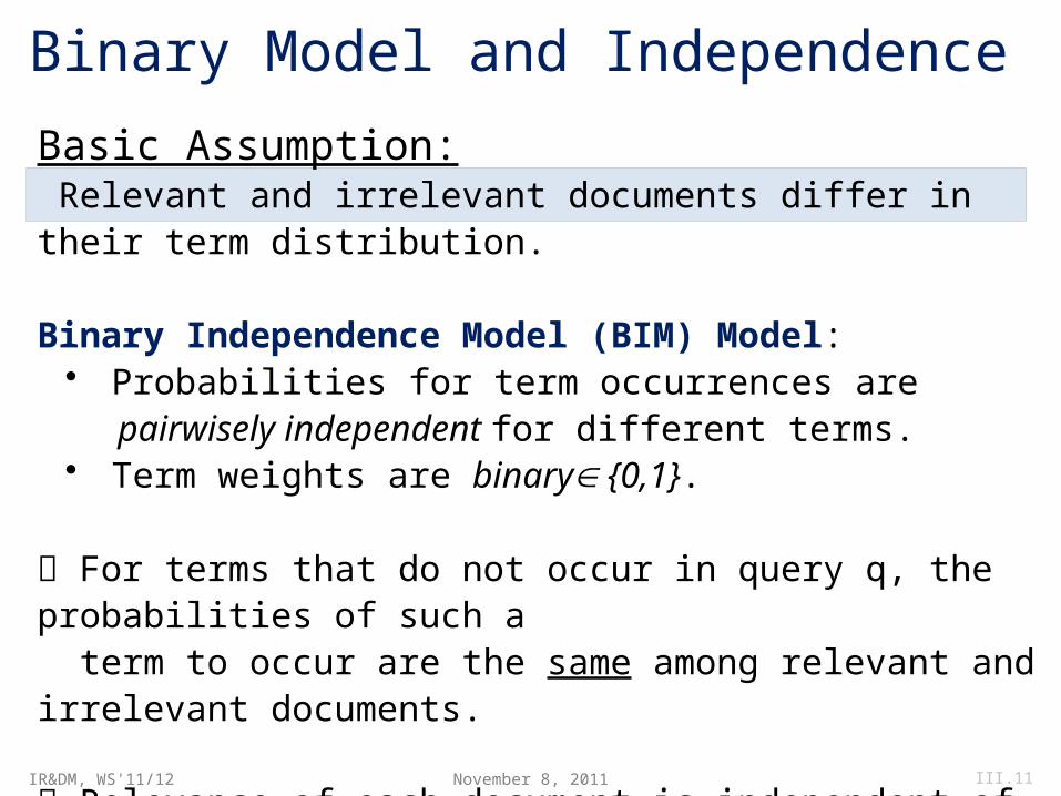
Binary Model and Independence
Basic Assumption: Relevant and irrelevant documents differ in their term distribution.
Binary Independence Model (BIM) Model:• Probabilities for term occurrences are
pairwisely independent for different terms.• Term weights are binary {0,1}.
For terms that do not occur in query q, the probabilities of such a term to occur are the same among relevant and irrelevant documents.
Relevance of each document is independent of the relevance of any other document.
November 8, 2011 III.11
IR&DM, WS'11/12
Ranking Proportional to Relevance Odds
]|0[
]|1[)|(),(
dRP
dRPdROqdsim
]0[]0|[
]1[]1|[
RPRdP
RPRdP (Bayes’ theorem)
(using odds for relevance)
]0|[
]1|[
RdP
RdP
m
i i
i
RdP
RdP
1 ]0|[
]1|[ (independence or linked dependence)
di = 1 if d includes term i, 0 otherwise
qi i
i
RdP
RdP
]0|[
]1|[ (P[di|R=1] = P[di|R=0] for i q)
Xi = 1 if random doc includes term i, 0 otherwise
qidi i
i
qidi i
i
RXP
RXP
RXP
RXP
]0|0[
]1|0[
]0|1[
]1|1[
November 8, 2011 III.12
IR&DM, WS'11/12
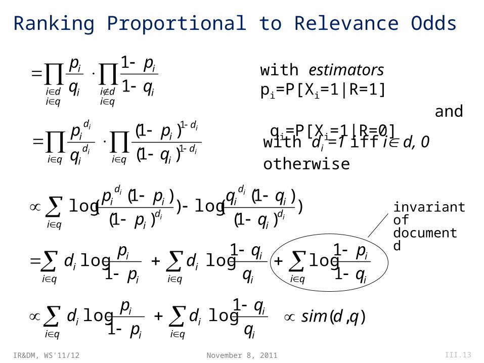
Ranking Proportional to Relevance Odds
with estimators pi=P[Xi=1|R=1] and qi=P[Xi=1|R=0]
qi
di
id
id
i
id
i
i
i
i
i
q
p
pp)
)1(
)1((log)
)1(
)1((log
qi qi i
i
i
i
qii
i
ii q
p
q
qd
p
pd
1
1log
1log
1log
qi i
i
qii
i
ii q
qd
p
pd
1log
1log ),( qdsim
qidi i
i
qidi i
i
q
p
q
p
1
1
qi
di
di
qid
i
di
i
i
i
i
q
p
q
p1
1
)1(
)1(with di =1 iff i d, 0 otherwise
invariant of document d
November 8, 2011 III.13
IR&DM, WS'11/12
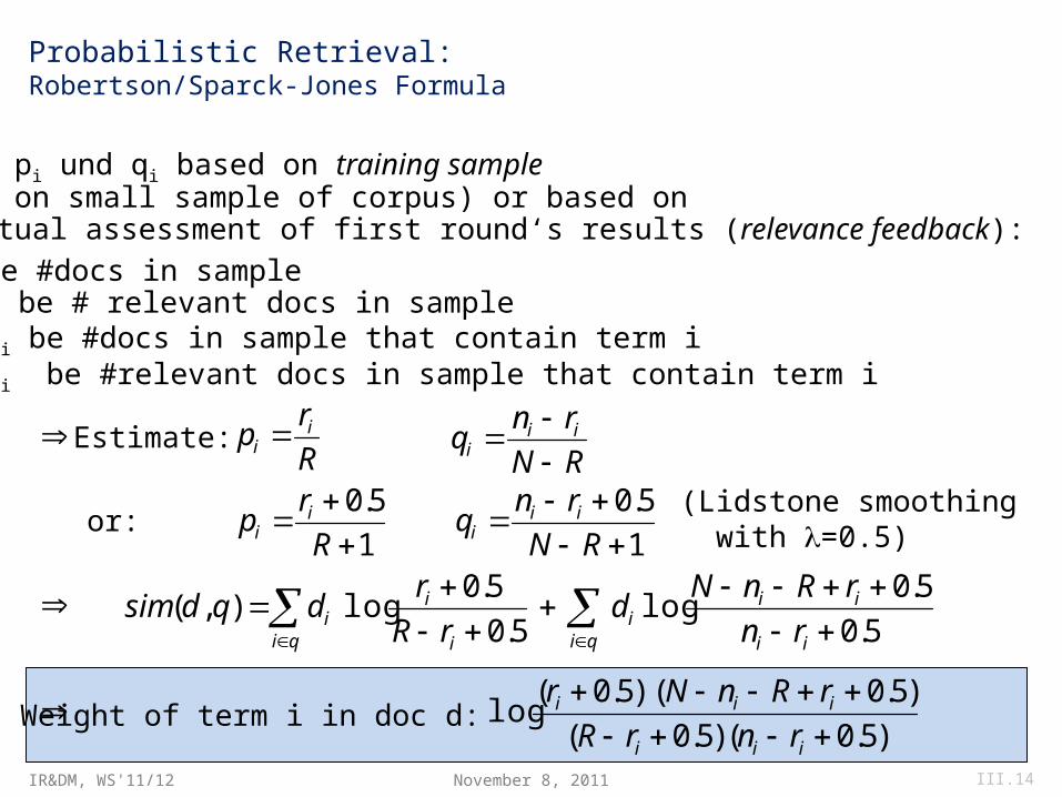
Probabilistic Retrieval:Robertson/Sparck-Jones Formula
Estimate pi und qi based on training sample(query q on small sample of corpus) or based onintellectual assessment of first round‘s results (relevance feedback):
Let N be #docs in sample R be # relevant docs in sample ni be #docs in sample that contain term i ri be #relevant docs in sample that contain term i
Estimate:R
rp i
i RN
rnq ii
i
or:1
5.0
R
rp i
i 1
5.0
RN
rnq ii
i
qi ii
iii
i
i
qii rn
rRnNd
rR
rdqdsim
5.0
5.0log
5.0
5.0log),(
Weight of term i in doc d:)5.0()5.0(
)5.0()5.0(log
iii
iii
rnrR
rRnNr
(Lidstone smoothing with =0.5)
November 8, 2011 III.14
IR&DM, WS'11/12
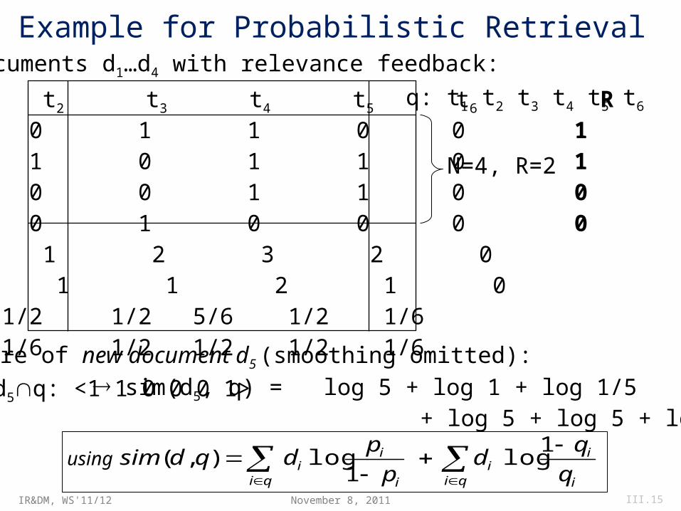
Example for Probabilistic RetrievalDocuments d1…d4 with relevance feedback:
t1 t2 t3 t4 t5 t6 Rd1 1 0 1 1 0 0 1d2 1 1 0 1 1 0 1d3 0 0 0 1 1 0 0d4 0 0 1 0 0 0 0ni 2 1 2 3 2 0 ri 2 1 1 2 1 0pi 5/6 1/2 1/2 5/6 1/2 1/6qi 1/6 1/6 1/2 1/2 1/2 1/6
N=4, R=2
q: t1 t2 t3 t4 t5 t6
Score of new document d5 (smoothing omitted):
d5q: <1 1 0 0 0 1> ® sim(d5, q) = log 5 + log 1 + log 1/5 + log 5 + log 5 + log 5
November 8, 2011 III.15
qi i
i
qii
i
ii q
qd
p
pdqdsim
1log
1log),(using

IR&DM, WS'11/12
Relationship to TF*IDF Formula
qi i
i
qii
i
ii q
qd
p
pdqdsim
1log
1log),(
Assumptions (without training sample or relevance feedback):• pi is the same for all i• most documents are irrelevant• each individual term i is infrequentThis implies:
•
•
•
qi
iqi i
ii dc
p
pd
1log
N
dfRXPq i
ii ]0|1[
ii
i
i
i
df
N
df
dfN
q
q
1
qi
iqi
ii idfddc log~ scalar product overthe product of tf anddampend idf valuesfor query terms
with constant c
November 8, 2011 III.16
IR&DM, WS'11/12
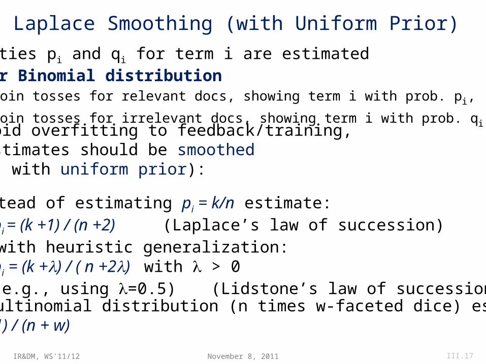
Laplace Smoothing (with Uniform Prior)Probabilities pi and qi for term i are estimatedby MLE for Binomial distribution(repeated coin tosses for relevant docs, showing term i with prob. pi,
repeated coin tosses for irrelevant docs, showing term i with prob. qi) To avoid overfitting to feedback/training,the estimates should be smoothed (e.g., with uniform prior):
Instead of estimating pi = k/n estimate:pi = (k +1) / (n +2) (Laplace’s law of succession)
or with heuristic generalization: pi = (k +) / ( n +2) with > 0 (e.g., using =0.5) (Lidstone’s law of succession)
And for Multinomial distribution (n times w-faceted dice) estimate:pi = (ki + 1) / (n + w)
November 8, 2011 III.17
IR&DM, WS'11/12
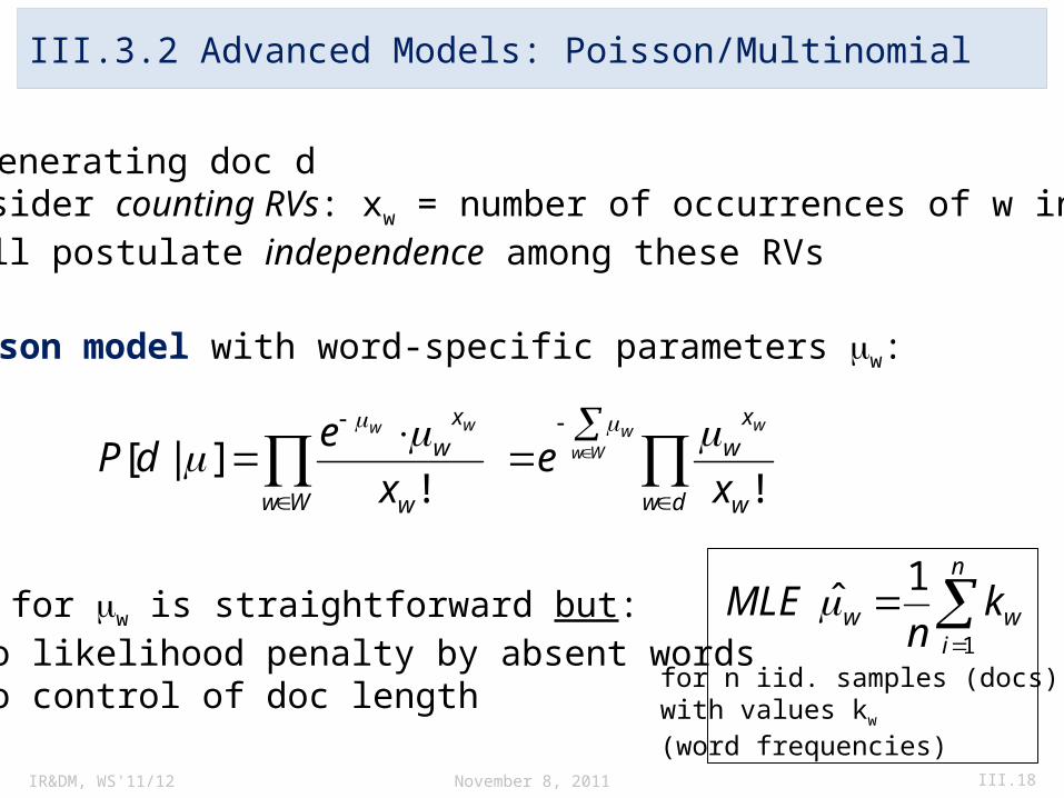
III.3.2 Advanced Models: Poisson/Multinomial
For generating doc d• consider counting RVs: xw = number of occurrences of w in d• still postulate independence among these RVs
Ww w
xw
x
edP
ww
!]|[
Poisson model with word-specific parameters w:
dw w
xw
xe
w
Www
!
MLE for w is straightforward but:• no likelihood penalty by absent words• no control of doc length
n
iww k
nMLE
1
1̂
for n iid. samples (docs)with values kw
(word frequencies)November 8, 2011 III.18
IR&DM, WS'11/12
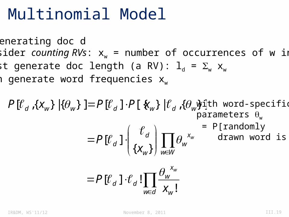
Multinomial Model
For generating doc d• consider counting RVs: xw = number of occurrences of w in d• first generate doc length (a RV): ld = w xw
• then generate word frequencies xw
}]{,|}[{][}]{|}{,[ wdwdwwd xPPxP with word-specificparameters w
= P[randomly drawn word is w]
dw w
xw
dd xP
w
!!][
Ww
xw
w
dd
w
xP
}{][
November 8, 2011 III.19
IR&DM, WS'11/12
Burstiness and the Dirichlet ModelProblem: • In practice, words in documents do not appear independently• Poisson/Multinomial underestimate likelihood of docs with high tf• “bursty” word occurrences are not unlikely:
• term may be frequent in doc but infrequent in corpus• for example, P[tf > 10] is low, but P[tf > 10 | tf > 0] is high
Solution: Two-level model • Hypergenerator: to generate doc, first generate word distribution in corpus (thus obtain parameters of doc-specific generative model)• Generator: then generate word frequencies in doc, using doc-specific model
November 8, 2011 III.20
IR&DM, WS'11/12
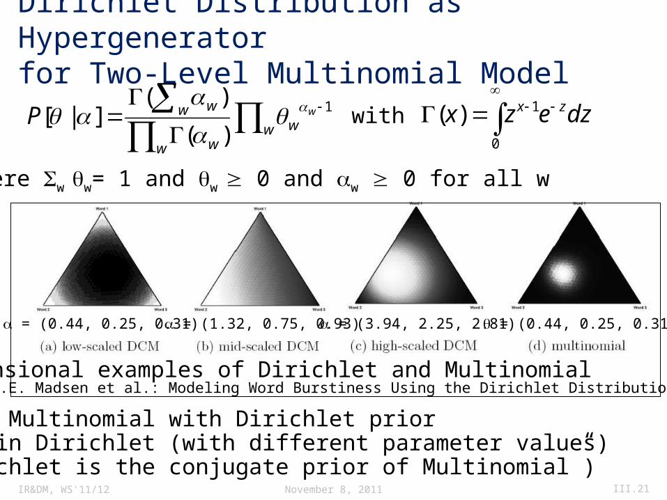
Dirichlet Distribution as Hypergeneratorfor Two-Level Multinomial Model
MAP of Multinomial with Dirichlet prioris again Dirichlet (with different parameter values)(“Dirichlet is the conjugate prior of Multinomial”)
w w
w w
w w wP 1
)(
)(]|[
where w w= 1 and w 0 and w 0 for all w
with
0
1)( dzezx zx
= (0.44, 0.25, 0.31) = (1.32, 0.75, 0.93) = (3.94, 2.25, 2.81) = (0.44, 0.25, 0.31)
3-dimensional examples of Dirichlet and Multinomial(Source: R.E. Madsen et al.: Modeling Word Burstiness Using the Dirichlet Distribution)
November 8, 2011 III.21
IR&DM, WS'11/12
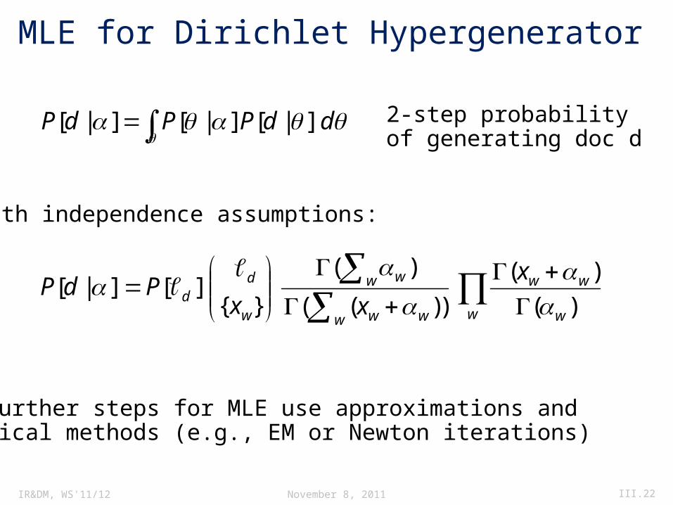
MLE for Dirichlet Hypergenerator
for further steps for MLE use approximations andnumerical methods (e.g., EM or Newton iterations)
ddPPdP ]|[]|[]|[ 2-step probabilityof generating doc d
w w
ww
w ww
w w
w
dd
x
xxPdP
)(
)(
))((
)(
}{][]|[
with independence assumptions:
November 8, 2011 III.22
IR&DM, WS'11/12
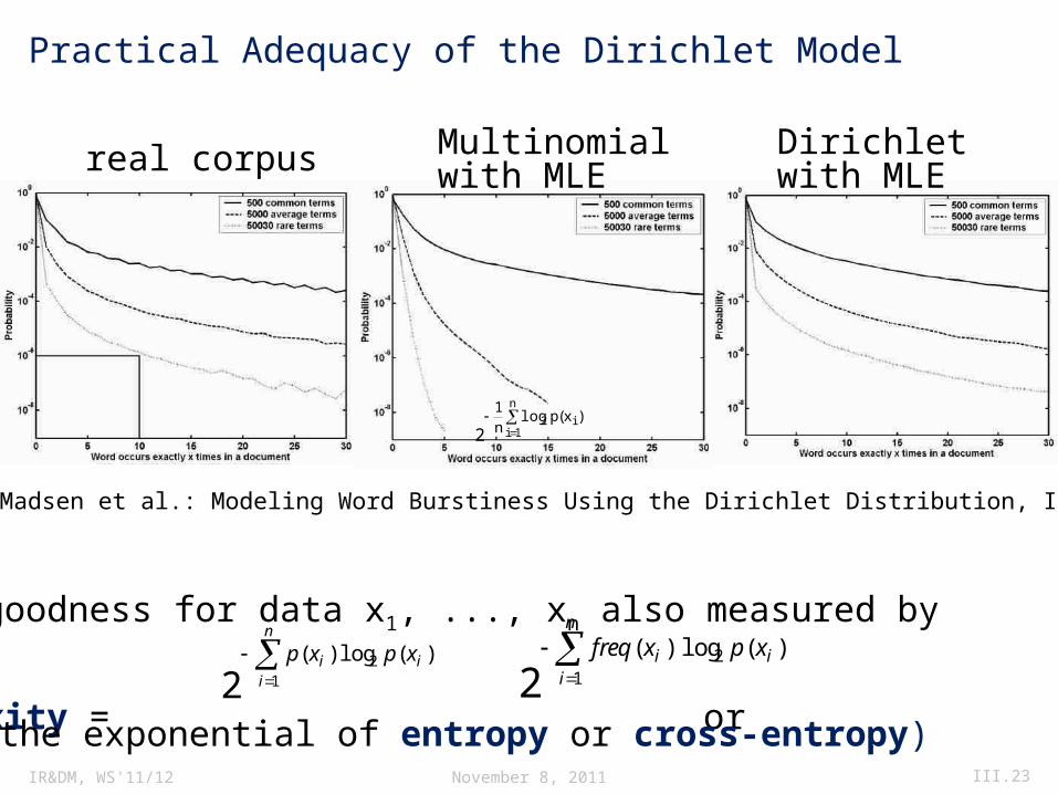
Practical Adequacy of the Dirichlet Model
n
1ii2 )x(plog
n1
2
real corpus Multinomialwith MLE
Dirichletwith MLE
Source: R. Madsen et al.: Modeling Word Burstiness Using the Dirichlet Distribution, ICML 2005
model goodness for data x1, ..., xn also measured by
perplexity = or
n
iii xpxfreq
12 )(log)(
2(i.e., the exponential of entropy or cross-entropy)
n
iii xpxp
12 )(log)(
2
November 8, 2011 III.23
IR&DM, WS'11/12
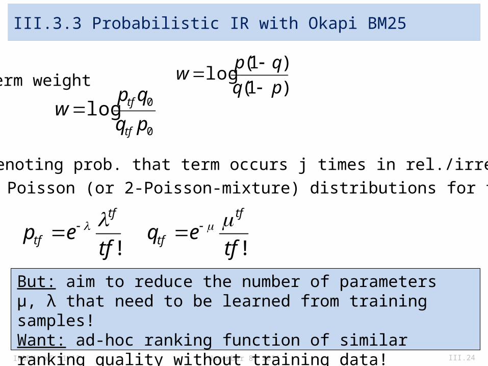
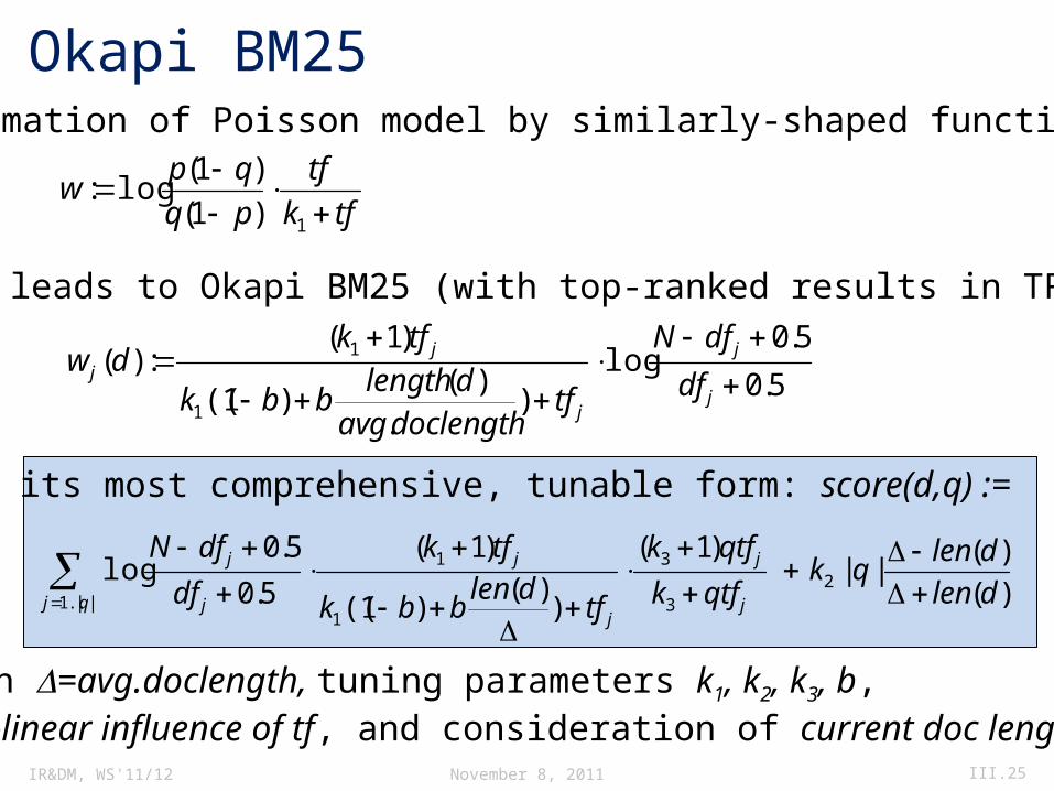
III.3.3 Probabilistic IR with Okapi BM25
)1(
)1(log
pq
qpw
Generalize term weight
into
with pj, qj denoting prob. that term occurs j times in rel./irrel. doc, resp.
0
0logpq
qpw
tf
tf
Postulate Poisson (or 2-Poisson-mixture) distributions for terms:
!tfep
tf
tf
!tf
eqtf
tf
November 8, 2011 III.24
But: aim to reduce the number of parameters μ, λ that need to be learned from training samples!Want: ad-hoc ranking function of similar ranking quality without training data!
IR&DM, WS'11/12
Okapi BM25
5.0
5.0log
).
)()1((
)1(:)(
1
1
j
j
j
jj df
dfN
tfdoclengthavg
dlengthbbk
tfkdw
Approximation of Poisson model by similarly-shaped function:
Finally leads to Okapi BM25 (with top-ranked results in TREC):
tfk
tf
pq
qpw
1)1(
)1(log:
with =avg.doclength, tuning parameters k1, k2, k3, b,non-linear influence of tf, and consideration of current doc length
Or in its most comprehensive, tunable form: score(d,q) :=
)(
)(||
)1(
))(
)1((
)1(
5.0
5.0log 2
3
3
1
1
||..1 dlen
dlenqk
qtfk
qtfk
tfdlen
bbk
tfk
df
dfN
j
j
j
j
j
j
qj
November 8, 2011 III.25
IR&DM, WS'11/12 November 8, 2011 III.26
5.0
5.0log
)1(:
1
1
j
j
j
jj df
dfN
tfk
tfkw
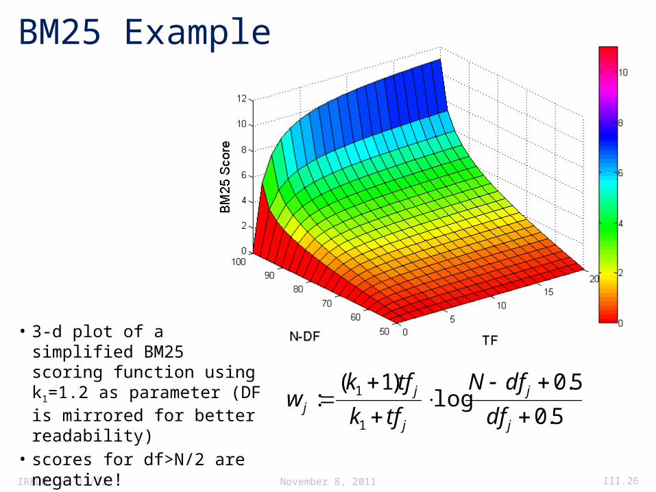
• 3-d plot of a simplified BM25 scoring function using k1=1.2 as parameter (DF is mirrored for better readability)
• scores for df>N/2 are negative!
BM25 Example
IR&DM, WS'11/12
III.3.4 Extensions to Probabilistic IR
One possible approach: Tree Dependence Model
a) Consider only 2-dimensional probabilities (for term pairs i,j)
fij(Xi, Xj)=P[Xi=..Xj=..]=
b) For each term pair i,j
estimate the error between independence and the actual correlation
c) Construct a tree with terms as nodes and the
m-1 highest error (or correlation) values as weighted edges
Consider term correlations in documents (with binary Xi) Problem of estimating m-dimensional prob. distribution P[X1=... X2= ... ... Xm=...] =: fX(X1, ..., Xm)
1 1 1 1 1
1 ...].....[......X iX iX jX jX mX
mXXP
November 8, 2011 III.27
IR&DM, WS'11/12
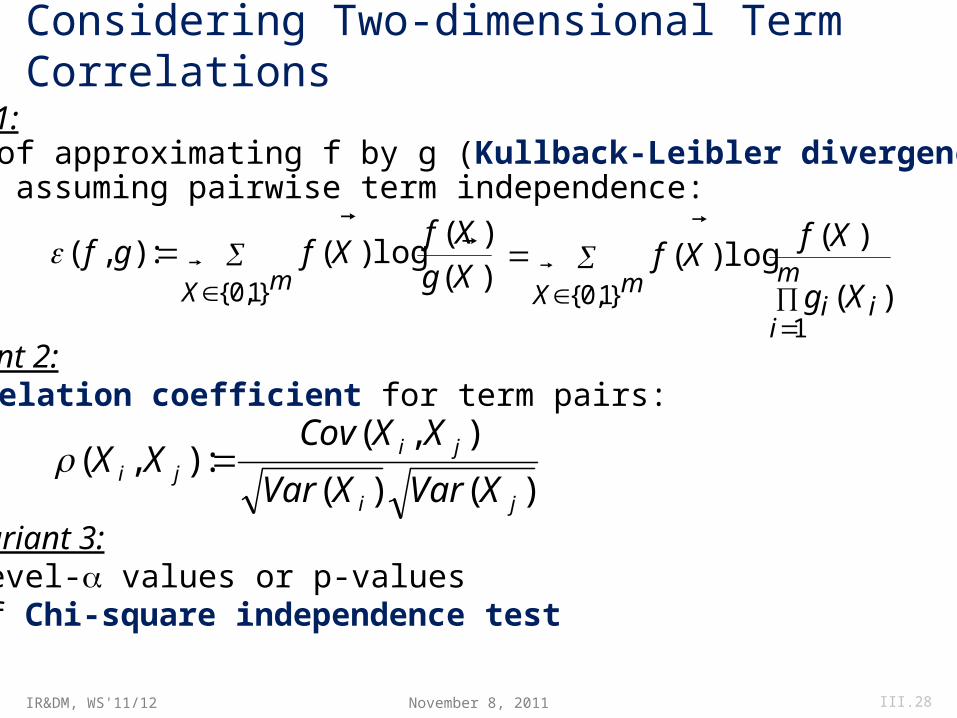
Considering Two-dimensional Term Correlations
Variant 1:Error of approximating f by g (Kullback-Leibler divergence)with g assuming pairwise term independence:
mX Xg
XfXfgf
}1,0{ )()(
log)(:),(
mX
m
iii Xg
XfXf
}1,0{1
)(
)(log)(
Variant 2:Correlation coefficient for term pairs:
)()(
),(:),(
ji
jiji
XVarXVar
XXCovXX
Variant 3:level- values or p-valuesof Chi-square independence test
November 8, 2011 III.28
IR&DM, WS'11/12
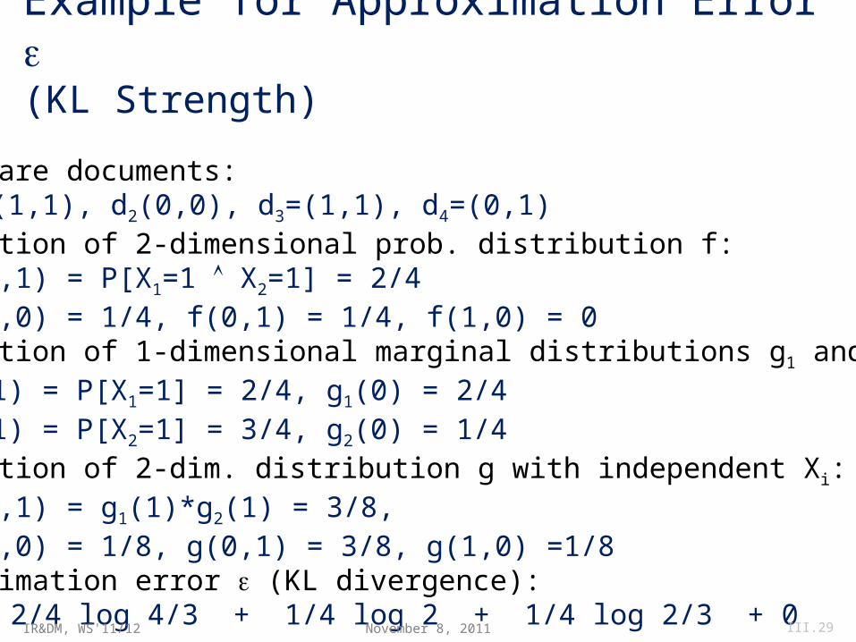
Example for Approximation Error (KL Strength)
m=2:given are documents: d1=(1,1), d2(0,0), d3=(1,1), d4=(0,1)estimation of 2-dimensional prob. distribution f: f(1,1) = P[X1=1 X2=1] = 2/4 f(0,0) = 1/4, f(0,1) = 1/4, f(1,0) = 0 estimation of 1-dimensional marginal distributions g1 and g2: g1(1) = P[X1=1] = 2/4, g1(0) = 2/4 g2(1) = P[X2=1] = 3/4, g2(0) = 1/4estimation of 2-dim. distribution g with independent Xi: g(1,1) = g1(1)*g2(1) = 3/8, g(0,0) = 1/8, g(0,1) = 3/8, g(1,0) =1/8approximation error (KL divergence): = 2/4 log 4/3 + 1/4 log 2 + 1/4 log 2/3 + 0
November 8, 2011 III.29
IR&DM, WS'11/12
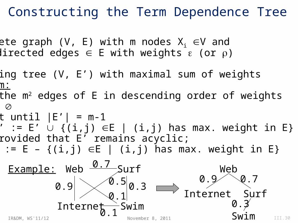
Constructing the Term Dependence TreeGiven: Complete graph (V, E) with m nodes Xi V and m2 undirected edges E with weights (or )Wanted: Spanning tree (V, E’) with maximal sum of weightsAlgorithm: Sort the m2 edges of E in descending order of weights E’ := Repeat until |E’| = m-1 E’ := E’ {(i,j) E | (i,j) has max. weight in E} provided that E’ remains acyclic; E := E – {(i,j) E | (i,j) has max. weight in E}
Example: Web
Internet
Surf
Swim
0.9
0.7
0.1
0.30.5
0.1
Web
Internet Surf
Swim
0.9 0.7
0.3November 8, 2011 III.30
IR&DM, WS'11/12
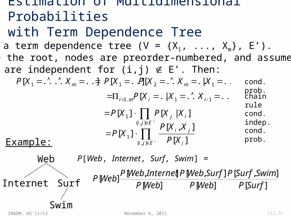
Estimation of Multidimensional Probabilities with Term Dependence Tree
Given is a term dependence tree (V = {X1, ..., Xm}, E’).Let X1 be the root, nodes are preorder-numbered, and assume thatXi and Xj are independent for (i,j) E’. Then:
..]....[ 1 mXXP
'),(
1 ]|[][Eji
ij XXPXP
'),(
1 ][
],[][
Eji i
ji
XP
XXPXP
Example:
Web
Internet Surf
Swim
P[Web, Internet, Surf, Swim] =
][],[
][],[
][],[
][SurfP
SwimSurfPWebP
SurfWebPWebPInternetWebP
WebP
..]|....[..][ 121 XXXPXP m
..]..|..[ 11..1 iimi XXXP
November 8, 2011 III.31
cond. prob.
chain rule
cond. indep.
cond. prob.
IR&DM, WS'11/12
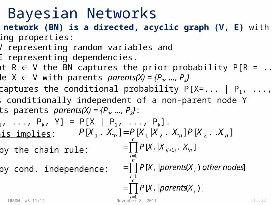
A Bayesian network (BN) is a directed, acyclic graph (V, E) withthe following properties:• Nodes V representing random variables and• Edges E representing dependencies.• For a root R V the BN captures the prior probability P[R = ...].• For a node X V with parents parents(X) = {P1, ..., Pk} the BN captures the conditional probability P[X=... | P1, ..., Pk].• Node X is conditionally independent of a non-parent node Y given its parents parents(X) = {P1, ..., Pk}: P[X | P1, ..., Pk, Y] = P[X | P1, ..., Pk].
This implies:
• by the chain rule:
• by cond. independence:
]...[]...|[]...[ 2211 nnn XXPXXXPXXP
n
inii XXXP
1)1( ]...|[
Bayesian Networks
n
iii nodesotherXparentsXP
1
]),(|[
n
iii XparentsXP
1
)](|[November 8, 2011 III.32
IR&DM, WS'11/12
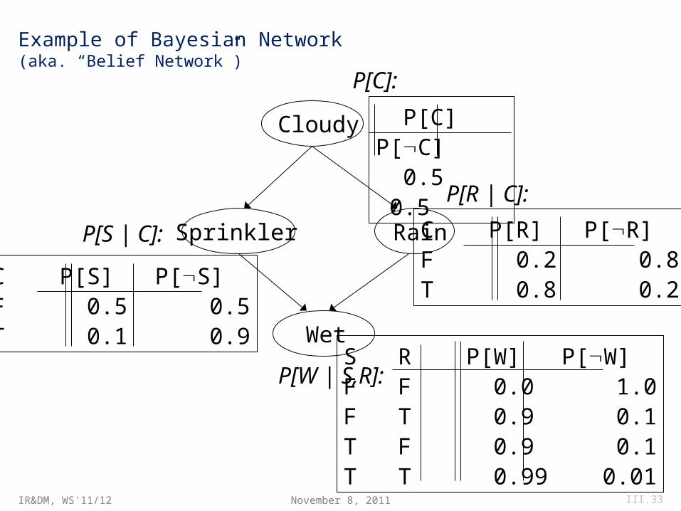
Example of Bayesian Network (aka. “Belief Network”)
Cloudy
Sprinkler Rain
WetS R P[W] P[W]F F 0.0 1.0F T 0.9 0.1T F 0.9 0.1T T 0.99 0.01
P[W | S,R]:
P[C] P[C] 0.5 0.5
P[C]:
C P[R] P[R]F 0.2 0.8T 0.8 0.2
P[R | C]:
C P[S] P[S]F 0.5 0.5T 0.1 0.9
P[S | C]:
November 8, 2011 III.33
IR&DM, WS'11/12
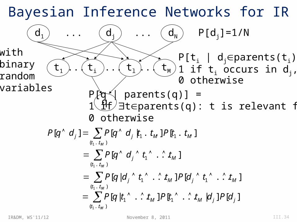
Bayesian Inference Networks for IRd1 dj dN... ...
t1 ti tM... ...
q
... tl
P[dj]=1/N
P[ti | djparents(ti)] = 1 if ti occurs in dj,0 otherwise
P[q | parents(q)] =1 if tparents(q): t is relevant for q,0 otherwise
withbinaryrandomvariables
]...[]...|[][ 11)...( 1
MMjtt
j ttPttdqPdqPM
]...[ 1
)...( 1
Mjtt
ttdqPM
]...[]...|[ 11
)...( 1
MjMjtt
ttdPttdqPM
][]|...[]...|[ 11
)...( 1
jjMMtt
dPdttPttqPM
November 8, 2011 III.34
IR&DM, WS'11/12
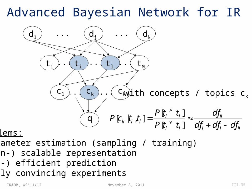
Advanced Bayesian Network for IRd1 dj dN
... ...
t1 ti tM... ...
q
... tl
c1 ck cK... ... with concepts / topics ck
Problems:• parameter estimation (sampling / training)• (non-) scalable representation• (in-) efficient prediction• fully convincing experiments
illi
il
li
lilik dfdfdf
df
ttP
ttPttcP
][
][],|[
November 8, 2011 III.35
IR&DM, WS'11/12
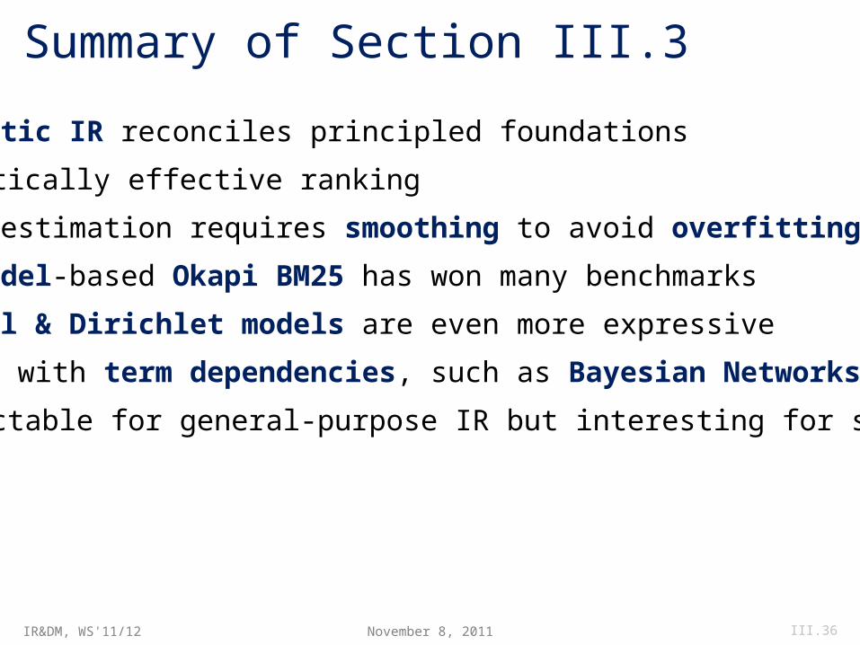
Summary of Section III.3
• Probabilistic IR reconciles principled foundations
with practically effective ranking
• Parameter estimation requires smoothing to avoid overfitting
• Poisson-model-based Okapi BM25 has won many benchmarks
• Multinomial & Dirichlet models are even more expressive
• Extensions with term dependencies, such as Bayesian Networks,
are intractable for general-purpose IR but interesting for specific apps
November 8, 2011 III.36
IR&DM, WS'11/12
Additional Literature for Section III.3• Manning/Raghavan/Schuetze, Chapter 11• K. van Rijsbergen: Information Retrieval, Chapter 6: Probabilistic Retrieval, 1979,
http://www.dcs.gla.ac.uk/Keith/Preface.html• R. Madsen, D. Kauchak, C. Elkan: Modeling Word Burstiness Using the
Dirichlet Distribution, ICML 2005 • S.E. Robertson, K. Sparck Jones: Relevance Weighting of Search Terms,
JASIS 27(3), 1976• S.E. Robertson, S. Walker: Some Simple Effective Approximations to the
2-Poisson Model for Probabilistic Weighted Retrieval, SIGIR 1994• A. Singhal: Modern Information Retrieval – a Brief Overview,
IEEE CS Data Engineering Bulletin 24(4), 2001• K.W. Church, W.A. Gale: Poisson Mixtures,
Natural Language Engineering 1(2), 1995• C.T. Yu, W. Meng: Principles of Database Query Processing for
Advanced Applications, Morgan Kaufmann, 1997, Chapter 9• D. Heckerman: A Tutorial on Learning with Bayesian Networks,
Technical Report MSR-TR-95-06, Microsoft Research, 1995• S. Chaudhuri, G. Das, V. Hristidis, G. Weikum: Probabilistic information retrieval
approach for ranking of database query results, TODS 31(3), 2006.
November 8, 2011 III.37