chapter i - · pdf filerahman and uddin (2009) indicated that education is a basic need of...
TRANSCRIPT

1
CHAPTER I
THE PROBLEM AND ITS BACKGROUND
Introduction
Education is the development of the endowed capacities in the individual,
which will enable him to control his environment and fulfill his possibilities to a
major extent. Education is a fostering, a nurturing and a cultivating process and
is attentive to all conditions of development. Furthermore, education is
considered also a social process and implies a social framework for social
individual development.
Rahman and Uddin (2009) indicated that education is a basic need of
human beings. It is also very important for the development of any country.
Education is the responsibility of the state and government who should make
every possible effort to provide it on an ever interesting and increasing scale in
accordance with the national resources.
In the rising seas of education’s changes, a group of people who have
been increasingly affected is at the instance of a much serious array of problems
regarding education. This group of people is composed of some 355 students of
the Department of Economics of the Polytechnic University of the Philippines.

2
For the past years, studies regarding the status and determining factors
regarding the academic performance of the students of PUP - Department of
Economics were seldom done and there were insufficient information about
these matters. Citations were apparent but there were no individual studies
conducted to discover the determinants affecting the level of academic
performances of students in DE.
Background of the Study
As a state university, PUP has always defended its stand that education is
an instrument for the development of the citizenry and for the enhancement of
nation building (PUP Handbook, revised 2007). Section 1.2.4 of the same
handbook indicates that in order to embody this philosophy, there is a need to
broaden opportunities for the intellectually qualified or scientifically inclined
through school fees within the reach of even the socio-economically
disadvantaged students. This reflects the nature of PUP as a higher education
institution which is primarily involved in catering the education needs of each
Filipino most specially the poor who wants to pursue his/her tertiary education in
one of the best universities in the country.
In line with the abovementioned information about PUP, its umbrella
department, the Department of Economics (DE) under the College of Economics,
Finance and Politics (CEFP) is aiming high in acquiring bright enrollees from
different parts of the country. DE is offering two undergraduate programs,
Bachelor of Science in Economics (BSE) and Bachelor of Science in Political

3
Economy (BSPE). Both programs have fair admission requirements unlike other
programs offered in the university like Bachelor of Science in Accountancy (BSA)
and Bachelor of Science in Computer Engineering (BSCS), which entails very
strict requisites upon admission. However, the retention policies of BSE and
BSPE in accordance with the college’s mission and vision are the true
determinants of the game.
PUP Website (www.pup.edu.ph) indicated the following policies of
retention of BSE and BSPE undergraduate students in DE.
A. On top of the academic delinquency rules of the University, incoming
third year students of the Department must:
1. Have a weighted average grade of at least 2.50 in:
A. All Economics, Mathematics, Statistics and English subjects
required in the first two years of the BSE curriculum;
B. All Economics, Mathematics, Statistics, English and political
science subjects required in the first two years of the BSPE
Curriculum;
2. Pass the qualifying exam to be administered by the Department, if
the student does not meet the minimum average grade requirement
stated in item A.1

4
3. Not have failed or dropped or withdrawn MT 135 (Algebra and
Trigonometry) or MT 205 (General Calculus) twice.
B. To advance to fourth year status, any student must:
4. Not have failed EC 130 (Mathematical Economics) or EC 140
(Economic Statistics) twice;
5. Not have been marked dropped or withdrawn in EC 130
(Mathematical Economics) or EC 140 (Economic Statistics) in two
semesters/summer, whether consecutive or not, in which the
student enrolled these subjects.
These are the reasons for which students in DE are well trained and
prepared to meet the needs of the real world. Many are not able to meet the
retention policies as for only 40 % - 50% are able to finish the two programs, thus
making them few of the best.
Many are speculating what factors affect the level of academic
performance of students in a tertiary institution like PUP. Numerous studies have
been done in order to know the factors that predict the academic performance of
students. All the researchers are settled in the conclusion that socio-economic
status, former school background and admission points affect college
performance. The Universities Admission Center (2006) reported that tertiary
institutions in Austria have found that a selection based on a student’s overall
academic achievement is the best single predictor of tertiary success.

5
With what the current trend is proposing, the researchers developed a
study to initiate a long-term significance in the admission and retention policies of
the DE. Since, the Department of Economics is increasingly becoming a seat of
excellence and versatility, it is by far necessary to come up with a study that will
test the relationships of High School Average, Type of School Graduated,
PUPCET Score, Family Income, Parents’ Occupation, Parents’ Education and
Chosen Program to the Academic Performance of the Students.
Conceptual Framework
This causality map shows the linkages between nodes represented by the
variables which reveal the influences or causalities between and among the
variables involved.
Father’s Education Mother’s Education Father’s Occupation Mother’s Occupation
PUPCET Score Average Family Income
High School Average
Course/Specialization Chosen
Academic Performance

6
The figure shows the causalities of the variables and the relationships
between and among key players.
The causality diagram starts from the top box which houses the variables
Father’s Education, Mother’s Education, Father’s Occupation and Mother’s
Occupation which indicate that these variables are the initial ones. The
researchers found out that these variables do not exhibit any related causalities
among other variables. The arrow connecting the first box from the immediate
box below it indicates that the variables in the second box are the outcomes of
the variables in the first box. These further means that PUPCET Score, Average
Family Income and High School Average are the results of the course happened
in box 1. The third box which houses Course/Specialization Chosen is the
progression of the variables in box 2 as indicated by the arrow connecting the
latter from the former. At on hand, PUPCET Score and High School Average are
two of the entry requirements of the Department of Economics in the admission
process. On the other hand, Average Family Income reveals the capacity of
students’ families in bringing their children into private or public schools in the
light of the tuition and miscellaneous fees. Since PUP is a government - owned
and non – profit university acclaimed as one the best universities offering high –
standard education for just PhP 12.00 per unit, the income of a family is a big
element in sending students to PUP. The box at the bottom represented by
Academic Performance is the final variable in which all the previous one will be
entering into. The academic performance of students will be determined based

7
on the Course/Specialization chosen by the students. In this way, the curriculum,
faculty – student relation and the general academic environment will serve as
steering wheels to generate academic performance with the accompaniment of
the variable being subjected by the researchers.
These were the causalities the researches built in order to make a solid
foundation on the inherent factors affecting academic performances of DE’s
freshmen students from 2009-2012.
The variables’ description below indicate the scope by which each variable
is treated and interpreted.
Average Family Income (AFI) comprises all the salary, wages and other
forms of income coming from different entities, jobs and other people including
donations and the like. These cover a time period of one month. This includes
donations, stipends and other forms of non-taxable financial resources.
The researchers’ a-priori expectation is since education has many forms
of purchase factors, a higher income means that a person has a greater
advantage in the light of spending than that of a person that has a lower income.
That is, if a student’s family has a high income, he/she will be able to invest in
his/her education by purchasing academic materials like books, journals and the
like which he/she can use to cater his/her needs for his/her study. This will
increase the chances of passing since he/she has a relatively more resources
than that of a student being a member of a family with lower income.

8
Mother’s Occupation (mooccu) and Father’s Occupation (faoccu) are the
determination whether the parents of the students are under the realms being
employed, self-employed and unemployed.
The researchers’ a priori expectation is that when a student has parents or
guardians who both are in employment sphere, he/she may have a better array
of opportunities from conception to adulthood. He/she will have better education
that in turn will translate into good academic performance. However, if a student
is in a family whose guardians are not employed, he/she is more prone in
becoming less productive and the array of opportunities that the former have is
not realized. This is supported by the Cultural Capital Theory which was used
Mastekaasa (2006) who argued that one could expect students from families who
are closest to academic culture to have greatest tertiary success.
Mother’s Education (moeduc) and Father’s Education (faeduc) refers to
the highest level of education the parents of the respondents have obtained.
The researchers’ a-priori expectation is that when the parents are educated
and have high attainments with regards to education, then the respondents
having these parents will eventually gain in their academics. Since education is
an element for human development, parents which are highly educated, their
sons and daughters are more inclined in having an academic ambiance which is
far more better than that of students whose parents are not educated or having
low attainments.

9
PUPCET Score (PS) refers to the scores the respondents obtained from
taking the Polytechnic University of the Philippines College Entrance Test
(PUPCET) in the process of admission in the university.
The researchers’ a-priori expectation is that since many researches have
concluded that academic history is the best predictor of academic success and
also since PUPCET is the reflection of the students’ initial performance, when a
student got a high PUPCET Score then he/she will have a greater chance of
excelling in class in terms of academics than that of his/her colleagues who
passed PUPCET yet obtained lower scores.
Type of School Graduated (SG) refers to the determination whether the
secondary school the students came from is either private or government-owned.
The researchers’ a priori expectation is that there are big differences
regarding the performances of secondary schools’ students in public schools as
compared to private ones. In a public school, the medley of a student is highly
heterogeneous. Nevertheless, in a private institution, it is noticeable that the
students generally came from middle and high income families. In addition,
public schools are conducting academic competitions and co-curricular activities
that private schools are lacking. And one big difference is that the teachers in
public schools have undergone intensive training and should have passed the
LET (Licensure Examination for Teachers) before teaching. These translate that
a student who came from a public school is more likely to obtain a better
academic background than that of a student coming from private fits of learning.

10
High School Average (HSA) refers to the average grade the students
obtained in the course of his/her 4th year residence in the secondary school
he/she came from.
The researchers’ a priori expectation is that. when a student has a good
academic history specifically having a high average , he/she is more likely to
have a consequent good academic performance in the present.
Course/Specialization Chosen (CSC) refers to whether the student is either
a BSE or BSPE undergraduate.
The researchers’ a priori expectation is that there are differences in the
academic performance of students in both undergraduate programs. Since the
two programs offer different curriculum, there is a possibility regarding the mode
of teaching and the substance of the curriculum might vary in many ways.
These inputs will be subjected as this study’s independent variables while the
Academic Performance (GWA) in terms of GWA is the dependent variable.
After subjecting the data, all treated values were statistically established with
the aid of SPSS (Software Packages for Social Sciences) V. 19 that was used in
order to test the correlation of the independent variables to the dependent
variables.
The resulting output is Academic Performance (GWA) that will interpret
DE’s Freshmen Students’ Academic Performances in the 1st semester of AY
2011-2012.

11
Theoretical Framework
In order to have a foundation to which this study held its grounds, the
researchers have utilized System’s theory input-output model developed by
Ludwig Von Bertalanffy in 1956 that explained and supported the results of this
study
. The theory, according to Koontz and Weihrich (1988) postulates that an
organized enterprise does not exist in a vacuum; it is dependent on its
environment in which it is established. They add that the inputs from the
environment are being received by the organization, which then transforms them
into outputs. As adapted in this study, the Freshmen students are the inputs with
different social economic backgrounds and are from various school backgrounds,
when they get into the organization which in this study is the Department of
Economics, the faculty-to-student involvement transforms them through the
process of teaching and learning and the students output is seen through their
academic performance. This further explains that the external and previous
environment is not a predictor of academic performance of students. The new
environment will determine their academic performance through the curriculum
offered, competence of professors, facilities, academic activities and over-all
academic environment.
Robbins (1980) argued that organizations were increasingly described as
absorbers, processors and generators and that the organizational system could
be envisioned as made up of several interdependent factors. System advocates,

12
according to Robbins (1980) have recognized that a change in any factor within
the organization has an impact on all other organizational or subsystem
components. Thus the inputs, the processors and the generators should function
well in order to achieve the desired outcome and as for this study is attaining
academic excellence. Saleemi (1997) in agreement with Robbins (1980) argued
that all systems must work in harmony in order to achieve the overall goals.
According to the input-output model, it is assumed that the students with high
social economic background and good school background will perform well if the
university facilities are good, the lecturers and the management of the university
is good which may not always be the case and this is the shortcoming of this
theory. According to Oso and Onen (2005), the interrelationships among parts of
a system have to be understood by all parties involved. This theory requires a
shared vision so that all people in the university have an idea of what they are
trying to achieve from all parties involved, a task that is not easy to achieve
Significance of Study
As an institutionalized study, this aimed to provide relevant and
substantial data and information about the current trend in the educational
track of Freshmen Students of the Department of Economics in the
Polytechnic University of the Philippines. In addition, this study will provide
answers to the most questionable arguments in the education sector, specifically
on the issue of the factors affecting academic performances of students.

13
Furthermore, this study will deliver relevant benefits to the following
sectors and institutions:
Government
As the sector that promotes the welfare and preserves the good of the
citizens, the government sees itself as the initial formulator of solutions to
different problems being faced by the country specifically in education and
learning.
This study is offering and delivering unparalleled benefits in the fields of
education, poverty alleviation, human development and income inequality
eradication that are currently prevailing in the Philippines.
Commission on Higher Education
With the inherent power to take over the administration of almost
8,000 state colleges and universities in the country, CHED is the prime
commandant of the administrations of these educational institutions. This
study will provide substantial and relevant information in the fields of
research and development that shall derive pertinent evolutions in the
Philippine Educational System.
National Statistics Office and National Statistics Coordinating Board
As the country’s engines of statistical data and resources, this
study will provide a never before seen and tested data that shall embody
the correlations between the factors that are not commonly related by

14
researchers and statisticians. In addition, this agency can utilize the
results for furthering the on-going studies of the government which focus
on education and youth empowerment.
Students
This study is also vital and indispensable to the morale of the students.
The students of the Department of Economics of the Polytechnic University of the
Philippines are the main beneficiaries of this study since the respondents were
from here.
The results are translated into descriptive and understandable way that
would enable the students to comprehend reality. Also, this study would motivate
the students to study harder for the researchers believe that the results of this
study will be favorable. The students would be able to know the reason why they
fail, pass, or more likely, have low grades.
Academe
Because the Polytechnic University of the Philippines is being endowed
with productive, intelligent and diligent students who embody the ideals of the
whole PUP system, this study aims to grant the students clear and transparent
look at the present status of their academic performance in the influences of the
factors involved.

15
Policy Formulation
The Polytechnic University of the Philippines, especially, the Department
of Economics would be able to have clear and practical policy ideas on the
course of accepting students. Through the results, the policy-making body of the
said university and of Department of Economics would have an in-depth analysis
on whether to increase or lessen scholarship grants and stipends to students. In
addition, the administration will be aware of the fallbacks of the recent policies
they have made and the windows for new and modern modes of retention
policies.
Admission Policies
The Department of Economics would be geared and guided by the
results of this study. This will help and serve as a basis for accepting
incoming freshmen students which in turn are the ones who are carrying
the ideals of DE. This study will stress points on the current admission
policies which at the first place are fair enough.
Retention Policies
This study would also help in the retention policies of DE for these
generated results that will reflect the current trend in DE. This would help
the administration in revising the retention policies that is to tighten or
loosen the already established requisites of passing and retention.

16
Scope and Limitations
This study focused on the effects of Course/Specialization Chosen, Type
of School Graduated From, PUPCET Score, Average Family Income, High
School Average, Father’s Education, Mother’s Education, Father’s Occupation
and Mother’s Occupation on the Academic Performance of Freshmen students of
the Department of Economics of the Polytechnic University of the Philippines for
the three consecutive 1st semesters of Academic Years 2009-2010, 2010-2011
and 2011-2012. Also, this study covered a total of 355 enrolled students in the 1st
year level in each 1st semester of the said academic years.
Due to the constraints set by the gathered data, the study focused
primarily in the determination of correlation of the following variables, specifically
Course/Specialization Chosen (CSC), Type of School Graduated From (SG),
PUPCET Score (PS), Average Family Income (AFI), High School Average
(HSA), Father’s Education (faeduc), Mother’s Education (moeduc), Father’s
Occupation (faoccu) and Mother’s Occupation (mooccu) to the academic
performance (GWA) of the students.
Statement of the Problem
This study generally focused on determining whether Academic
Performance (GWA) of DE’s Freshmen Students in the 1st Semesters of A.Y.
2009-200, A.Y. 2010-2011 and A.Y. 2011-2012 is significantly correlated to Type
of School Graduated From (SG), PUPCET Score (PS), Course/Specialization
Chosen (CSC), High School Average (HSA), Father’s Education (faeduc),

17
Mother’s Education (moeduc), Father’s Occupation (faoccu) and Mother’s
Occupation (mooccu) and Average Family Income (AFI).
Moreover, this study tackled and answered the following specific questions:
1. What are the demographic profiles of DE’s Freshmen students in
Academic Year 2009-2010, Academic Year 2010-2011 and Academic
Year 2011-2012 in terms of the following:
a. Course/Specialization Chosen (CSC)
b. High School Average (HSA)
c. Type of School Graduated From (SG)
d. PUPCET Score (PS)
e. Average Family Income (AFI)
f. Father’s Occupation (faoccu)
g. Mother’s Occupation (mooccu)
h. Father’s Education (faeduc)
i. Mother’s Education (moeduc)
2. Are there significant differences in the academic performances of DE
students in Academic Year 2009-2010, Academic Year 2010-2011 and
Academic Year 2011-2012 in terms of the following:
a. Course/Specialization Chosen (CSC)
b. Type of School Graduated From (SG)
c. High School Average (HSA)
d. PUPCET Score (PS)
e. Average Family Income (AFI)

18
f. Father’s Occupation (faoccu)
g. Mother’s Occupation (mooccu)
h. Father’s Education (faeduc)
i. Mother’s Education (moeduc)
3. Are there correlations between DE students’ academic performance in
Academic Year 2009-2010, Academic Year 2010-2011 and Academic
Year 2011-2012 in terms of the following:
a. Course/Specialization Chosen (CSC)
b. Type of School Graduated From (SG)
c. High School Average (HSA)
d. PUPCET Score (PS)
e. Average Family Income (AFI)
f. Father’s Occupation (faoccu)
g. Mother’s Occupation (mooccu)
h. Father’s Education (faeduc)
i. Mother’s Education (moeduc)
Objectives of the Study
General Objective
The primary objective of this research work is to determine whether there
are correlations between Type of School Graduated From (SG), PUPCET Score
(PS), Course/Specialization Chosen (CSC), High School Average (HSA),
Father’s Education (faeduc), Mother’s Education (moeduc), Father’s Occupation

19
(faoccu) and Mother’s Occupation (mooccu) and Average Family Income (AFI) to
Academic Performance (GWA) of DE’s Freshmen Students in the 1st Semesters
of A.Y. 2009-200, A.Y. 2010-2011 and A.Y. 2011-2012
Specific Objectives
1. To know the demographic profiles of DE’s Freshmen students in
Academic Year 2009-2010, Academic Year 2010-2011 and Academic
Year 2011-2012 in terms of the following:
a. Course/Specialization Chosen (CSC)
b. High School Average (HSA)
c. Type of School Graduated From (SG)
d. PUPCET Score (PS)
e. Average Family Income (AFI)
f. Father’s Occupation (faoccu)
g. Mother’s Occupation (mooccu)
h. Father’s Education (faeduc)
i. Mother’s Education (moeduc)
2. To discover whether there are significant differences in the academic
performances of DE students in Academic Year 2009-2010, Academic
Year 2010-2011 and Academic Year 2011-2012 in terms of the
following:
a. Course/Specialization Chosen (CSC)
b. Type of School Graduated From (SG)
c. High School Average (HSA)

20
d. PUPCET Score (PS)
e. Average Family Income (AFI)
f. Father’s Occupation (faoccu)
g. Mother’s Occupation (mooccu)
h. Father’s Education (faeduc)
i. Mother’s Education (moeduc)
3. To see if there are correlations to DE students’ academic performance
in Academic Year 2009-2010, Academic Year 2010-2011 and
Academic Year 2011-2012 in terms of the following:
a. Course/Specialization Chosen (CSC)
b. Type of School Graduated From (SG)
c. High School Average (HSA)
d. PUPCET Score (PS)
e. Average Family Income (AFI)
f. Father’s Occupation (faoccu)
g. Mother’s Occupation (mooccu)
h. Father’s Education (faeduc)
i. Mother’s Education (moeduc)
21
Statement of Hypotheses
The following null hypotheses were formulated in line the statement of the
problem presented in order to meet the objectives of the study:
1. There is no significant correlation between Academic Performance and
Course/Specialization Chosen in A.Y. 2009-2010.
2. There is no significant correlation between Academic Performance and
High School Average in A.Y. 2009-2010.
3. There is no significant correlation between Academic Performance and
Type of School Graduated From in A.Y. 2009-2010.
4. There is no significant correlation between Academic Performance and
PUPCET Score in A.Y. 2009-2010.
5. There is no significant correlation between Academic Performance and
Average Family Income in A.Y. 2009-2010.
6. There is no significant correlation between Academic Performance and
Father’s Occupation in A.Y. 2009-2010.
7. There is no significant correlation between Academic Performance and
Mother’s Occupation in A.Y. 2009-2010.
8. There is no significant correlation between Academic Performance and
Father’s Education in A.Y. 2009-2010.

22
9. There is no significant correlation between Academic Performance and
Mother’s Education in A.Y. 2009-2010
10. There is no significant correlation between Academic Performance and
Course/Specialization Chosen in A.Y. 2010-2011.
11. There is no significant correlation between Academic Performance and
High School Average in A.Y. 2010-2011.
12. There is no significant correlation between Academic Performance and
Type of School Graduated From in A.Y. 2010-2011.
13. There is no significant correlation between Academic Performance and
PUPCET Score in A.Y. 2010-2011.
14. There is no significant correlation between Academic Performance and
Average Family Income in A.Y. 2010-2011.
15. There is no significant correlation between Academic Performance and
Father’s Occupation in A.Y. 2010-2011.
16. There is no significant correlation between Academic Performance and
Mother’s Occupation in A.Y. 2010-2011.
17. There is no significant correlation between Academic Performance and
Father’s Education in A.Y. 2010-2011.
18. There is no significant correlation between Academic Performance and
Mother’s Education in A.Y. 2010-2011

23
19. There is no significant correlation between Academic Performance and
Course/Specialization Chosen in A.Y. 2011-2012.
20. There is no significant correlation between Academic Performance and
High School Average in A.Y. 2011-2012.
21. There is no significant correlation between Academic Performance and
Type of School Graduated From in A.Y. 2011-2012.
22. There is no significant correlation between Academic Performance and
PUPCET Score in A.Y. 2011-2012.
23. There is no significant correlation between Academic Performance and
Average Family Income in A.Y. 2011-2012.
24. There is no significant correlation between Academic Performance and
Father’s Occupation in A.Y. 2011-2012.
25. There is no significant correlation between Academic Performance and
Mother’s Occupation in A.Y. 2011-2012.
26. There is no significant correlation between Academic Performance and
Father’s Education in A.Y. 2011-2012.
27. There is no significant correlation between Academic Performance and
Mother’s Education in A.Y. 2011-2012.

24
CHAPTER II
REVIEW OF RELATED LITERATURE AND STUDIES
This chapter exhibited the related works, literature, studies and scholarly
pieces that constitute the foundation of the study. Specifically, included here are
local and foreign literature and studies that will serve as basis that will develop
the grounds for experimentation and testing.
Foreign Literature
There are certain principles and theories that can justify and support to the
role of socio-economic factors and other indicators, which affect academic
performance of students especially in tertiary education.
Social economic status is most commonly determined by combining
parents’ educational level, occupational status and income level (Jeynes, 2002;
McMillan & Western, 2000).
According to McMillan and Westor (2002) social economic status is
comprised of three major dimensions: education, occupation and income and
therefore in developing indicators appropriate for high education context,
researchers should study each dimension of social economic status separately.
They add that education, occupation and income are moderately correlated

25
therefore it is inappropriate to treat them interchangeably in the higher education
context. The researcher therefore should review literature on each of the
components of social economic status in relation to academic performance.
Family income, according to Escarce (2003) has a profound influence on the
educational opportunities available to adolescents and on their chances of
educational success. Escarce (2003) adds that due to residential stratification
and segregation, low-income students usually attend schools with lower funding
levels, have reduced achievement motivation and much higher risk of
educational failure. When compared with their more affluent counterparts, low-
income adolescents receive lower grades, earn lower scores on standardized
test and are much more likely to drop out of school. Considine and Zappala
(2002) indicated that children from families with low income are more likely to
exhibit the following patterns in terms of educational outcomes; have lower levels
of literacy, innumeracy and comprehension, lower retention rates, exhibit higher
levels of problematic school behavior, are more likely to have difficulties with their
studies and display negative attitudes to school. King and Bellow used parents’
occupation as a proxy for income to examine the relationship between income
and achievement and found that children of farmers had fewer years of schooling
than children of parents with white-collar jobs. They also determined that the
schooling levels of both parents had a positive and statistically significant effect
on the educational attainment of Peruvian children. They observe that the higher
the attainment for parents, then the greater their aspirations for children.

26
Rodriguez (2007) considers that academic failure as the situation in which
the subject does not attain the expected achievement according to his or her
abilities resulting in an altered personality which affects all other aspects of life.
Similarly, Tapia notes that while the current Educational System perceives that
the students fails if she or she does not pass, more appropriate for determining
academic failure is whether the students perform below his or her potential.
In 2007, Ruby Payne indicated that low achievement can be closely
correlated with poverty. In the United States, students who come from
impoverished families are more likely to have problems in school than students
who come from middle-class or upper class families. Unfortunately, the United
States has very high rates of childhood poverty. Furthermore, it is very difficult for
the impoverished families to escape poverty once they are in it.
According to the Cultural capital Theory, one could expect students from
families who are closest to the academic culture to have greatest success. In
agreement with this theory, Combs (1985) concluded that, in all nations, children
of parents high on the educational, occupation and social scale have far better
chance of getting into good secondary schools and from there into the best
colleges and universities than equally bright children of ordinary works and
farmers. Dills (2006) agreed that student from the bottom quartile consistently
perform below students from the top quartile of socio-economic status.
Another group of performance-determining factors are the social/family
factors. There is an ever-increasing awareness of the importance of the parents’

27
role in the progress and educational attainment of the students. Simmons
considers family background as the most important and most weighty factor in
determining the academic performance attained by the student. Among family
factors of greatest influence are social class variables and the educational and
family environment.
Bettinger (2004) stated that financial aid could influence collegiate
success in both direct and indirect ways. Directly, financial aid could help defray
tuition and other costs, thus making persistence from one term to the next
feasible. However, financial aid could have additional indirect effects by
influencing some of the factors known to be related to student success.
Academic preparation and studying in college are thought to be the most
important factors in student success.
Local Literature
The Commission in Higher Education (CHED) stressed that there will be
almost 590,000 college graduates in the Philippines. This is low because many
fail to complete the undergraduate course program a student has chosen.
(www.ched.gov.ph)(August 3, 2012)
This is the reason for which the Department of Education (DepEed) has
been entering into the realms of financial assistance and scholarship grants in
order to support the need of the pursuing students and those who want to pursue
their studies in college. Clearly, as what this statement had said, socio-economic
status is a determinant in the retention and upon admission itself.

28
The basis for quality education in the Philippines is clearly defined as the
sustainability and excellence of students with the accompaniment of quality
teaching and instructions. (www.deped.gov,ph)(August 4, 2012)
Senator Edgardo J. Angara (LDP) revealed a 3-point agenda to revive the
quality of education, as well as to address the problem of Filipino
competitiveness in the global work force industry. “Higher education has now
become international. Today, we train people not just for our work force need.
We train them for the world. And when people from other countries come here,
they will come here to look for the global-quality graduates," said Angara at the
20TH Accrediting Agency of Chartered Colleges and Universities in
the Philippines (AACCUP)”. Consciously and systematically, bring up our
academic standards more than the ordinary to meet international standard. The
skills and qualifications of students must elevate for the reason that they are
element to their institution and to the country,” Angara said. Angara also said that
CHED was intentional to be the vehicle to push the development of higher
education rather than simply serve as a regulatory body.
Foreign Studies
Different studies, investigations and researches were conducted by
different institutions outside the Philippines, which are related to the study being
undertaken by the researchers.

29
Based on a study conducted by Kyoshaba Martha in 2009 at Uganda
Christian University, she made the following conclusions; A’ level and diploma
admission points are the most objective way to select just a few students from a
multitude of applicants for the 12 limited slots available at universities in Uganda.
Parents’ social economic status is important because parents provide high levels
of psychological support for their children through environments that encourage
the development of skills necessary for success at school. That location,
ownership and academic and financial status of schools do count on making a
school what it is and in turn influencing the academic performance of its students
because they set the parameters of a students’ learning experience.
College students have many obstacles to overcome in order to achieve
their optimal academic performance. It takes a lot more than just studying to
achieve a successful college career. Different stressors such as time
management, financial problems, sleep deprivation, social activities, and for
some students even having children, can all pose their own threat to a student’s
academic performance. The way that academic performance is measured is
through the ordinal scale of grade point average (GPA). A student’s GPA
determines many things such as class rank and entrance to graduate school.
Much research has been done looking at the correlation of many stress factors
that college students’ experience and the effects of stress on their
GPA.(http://www.oppapers.com/essays/Factors-Affecting-AcademicPerformance/
624248) (February 13, 2012)

30
Eamon (2005) indicated that in most of the studies done on academic
performance of students, it is not surprising that social economic status is one of
the major factors studied while predicting academic performance. Jeynes (2002)
pointed out that low social economic status prevents access to vital resources
and creates additional stress at home.
The study done by Graetz (2000) on social economic status in education
research, found that social economic background remains one of the major
sources of educational inequality and that one’s educational success depends
very strongly on the social economic status of one’s parents. Considine and
Zappala (2002) agree with Graetz (2000). Their study on the influence of social
and economic disadvantage in the academic performance of school students in
Australia found that families where the parents are advantaged socially,
educationally and economically foster a higher level of achievement in their
children. They found that socially advantage parents provide higher levels of
psychological support for their children through environments that encourage the
development of skills necessary for success at school.
A study at Alberta, Canada as published in 2012 by Russel Horswill
concluded that school building condition and school’s geographical location do
not influence academic performances. Interactive effect of school building
condition and school’s geographical location also generated an insignificant
result. Horswill (2012) posited that even though this study’s conclusion is not
aligned with other studies’ findings, he reiterated that Alberta, Canada is the best
province in terms of academic performance of grade school and secondary

31
school students. Horswill (2012) added that since the government has invested
so much in the quality of education in Canada, the factors he used did not
influence that fact.
Kwesiga (2002) and Sentamu (2003) found that the type of school a child
attends influences educational outcomes. They also reported that the school a
child attends affects academic performance. It was also confirmed by Minnesota
measures (2007) that the most reliable predictor of student success in college is
the academic preparation of students in high school. Sentamu (2003) also
agrees that the type of school one attend affects academic performance because
schools influence learning in the way content is organized and in the teaching,
learning and assessment procedures.
On the contrary, Pedrosa et al. (2006) in their study on educational and
social economic background of undergraduates and academic performance at a
Brazilian university, they found that students coming from disadvantaged
socioeconomic and educational homes perform relatively better than those
coming from higher socioeconomic and educational strata. They called this
phenomenal educational resilience. This could be true considering that different
countries have different parameters of categorizing social economic status. What
a developed country categorizes as low social economic status may be different
from the definition of low social economic status of a developing country.
Additionally, students do not form a homogenous group and one measure of
social economic disadvantage may not suit all sub groups equally.

32
Hansen and Mastekaasa (2006) showed the same view, when they
studied the impact of class origin on grades among all first year students and
higher level graduates in Norwegian universities. Their analysis showed that
students originating in classes that score high with respect to cultural capital tend
to receive the highest grades.
A study suggested that financial aid has positive effects not only on
academic performance but also on other behaviors likely to support college
success and social benefits. Part of the difficulty in understanding the impact of
financial aid on college achievement and persistence is that other factors, such
as academic preparation, are also important determinants of college outcomes,
making it difficult to isolate the impact of aid from these other factors. Moreover,
students who receive financial aid tend to have different characteristics than non-
recipients, thereby causing selection bias in straightforward comparisons of
recipients to non-recipients. (Kuh et al., 2007)
An argument explained by Geiser and Santelices (2007) at Uganda
Christian University, that high school grades or admission points reflects a
student’s cumulative performance over a period of years and that is why they are
consistently the best predictor of college success. They also emphasize high
school grades focuses on the mastery of specific skills and knowledge required
for college-level work. In addition, it could also owe to the fact that the students
who had previously performed well continue to do so because they have a strong
potential to easily catch up with university work and they are motivated to do so.

33
In a study in 2000 Trockel, Barnes, and Egget found, nutrition is also a
problem with college students. Students may have difficulty finding the time to
cook adequate meals. Most students are just learning to live on their own, and
learning to cook can prove to be a challenge. Finding time to go to the grocery
store once every couple of weeks can be a demanding task. Little storage space
is available in the average dorm room, and food storage may not be possible at
all.
A research study conducted at the University of North Carolina at
Charlotte on 2003 found out that there are many factors that can cause stress
and influence a student’s academic performance and therefore affect his or her
overall GPA. The factors include exercise, nutrition, sleep, and work and class
attendance. A college student may find him or herself in a juggling act, trying to
support a family, taking care of job responsibilities, and at the same time trying to
make the most of the college career. All of these factors can affect the grades of
students, which ultimately affect the rest of their lives.
Local Studies
In a study conducted by the School of Economics of De La Salle
University in 2009 as indicated in Volume II of Policy Brief, based on household
data, it was empirically verified that the magnitude of household income does not
significantly affect school participation. Tereso Tullao Jr. and Rivera, John Paulo
(2009) found out that as the income of households’ increases, they will also
increase their expenditures on normal goods and services including education.

34
However, primary education in the Philippines is widely publicly provided. Hence,
income will be allocated to non-educational expenditures. It might also be the
case that households base their decisions including whether to send their
children to school on permanent income rather than transitory income. The
income reported by households when the survey was conducted was transitory
income and may have been lower than what the household normally earns over
a longer period of time.
Policy Brief (2009) indicated the impact of population growth on school
participation - as the family size increases, school participation declines. This
result is a very strong argument for the need to manage the population growth of
the country; otherwise, it may adversely affect the human capital formation at the
household level in both urban and rural area. Since school participation is
influenced negatively by family size, the issue of rapid population growth can
significantly impede the ability of the country to maintain its competitive edge in
the production of highly educated and skilled workers in the future since poorer
and bigger families are investing less in human capital. Hence, there is really a
need to address the issue of population growth.
Tereso Tullao Jr. and Rivera, John Paulo (2009) added that another
important result of the study is the positive impact of the employment status and
educational attainment of the household head to school participation. For the
earlier, school participation can be assured if the household head is employed.
For the latter, such result emanates from the culture of education where
educated parents beget more educated children. This dictum does hold true in

35
Pasay and Eastern Samar where the estimated coefficients have shown
significant impact on school participation evidencing that parent’s educational
attainment is indeed relevant as an inducer of academic performance.
Synthesis
This part summarized the highlights of the studies and literatures the
researchers utilized on the process of doing this study.
Mcmillan and Western indicated that social economic status is said to be
the most commonly determined by combining parents’ educational and level as
well as occupational status. It is supported by McMillian and Westor who says
that education, occupation and income are moderately correlated thus it is
inappropriate to treat them interchangeably in the higher education context.
However, the effects of family income to the academic performance,
Scarce has profound influence on the educational opportunities available to
students are on their scholastic success. Considine and Zappala indicated that
children from low income families relatively exhibit more patterns in terms of
education outcomes like having a lower literacy, lower retention rates and the
like. King and Bellow used parents’ occupation as a representation for income to
examine the relationship between income and achievement in education. They
concluded that the higher the attainment of parents the greater their ambitions for
their children.

36
In the US, students who are from underprivileged families are more
relatively to have problems in school than students who come from middle class
or upper class families.
Cultural Capital theory states that there are significant and notable
differences in academic performance of students when the level of socio-
economic status of their families is concerned. The rich will still perform better
even though the poor has the intelligence. Thus, this theory cites the importance
of investment on education. This theory was supported by Combs that those
children with parents having higher education, occupation and social scale have
a better chance to attain a higher quality of education.
Bettinger stated that financial aid could have additional indirect effects by
influencing some of the factors known to be related to student success.
Academic preparation and studying in college are thought to be the most
important factors in student success.
According to Kwesiga and Sentanu the type of school a child attends
influences educational outcomes. It was agreed by Minnesota that the most
reliable predictor of students’ success in college is the academic preparation of
students in high school. In addition, Geiser and Sentilices explained that high
school grades focuses on the mastery of specific skills and knowledge required
for the level of education in college.
Moreover, Pedrosa et al., in their study on educational and social
economic background of undergraduates and academic performance found that

37
students coming from disadvantaged socioeconomic and educational homes
perform relatively better than those coming from higher socioeconomic and
educational strata.
In addition, a study conducted by the School of Economics of De La Salle
University in 2009 as indicated in Volume II of Policy Brief, verified that the
magnitude of household income does not significantly affect school participation.
Tullao and Rivero concluded that as the income of household increases, they will
also increase their expenditure on normal goods and services which include
education.
The Commission on Higher Education (CHED) clearly stated that socio-
economic status is a determinant in the retention and upon admission itself.
A study conducted at Alberta, Canada in 2012, concluded that there are
no significant relationship school facilities and school location held for academic
performance.
Policy Brief indicated the impact of population growth on school
participation - as the family size increases, school participation declines. Since
school participation is influenced negatively by family size, the issue of rapid
population growth can significantly impede the ability of the country to maintain
its competitive edge in the production of highly educated and skilled workers in
the future since poorer and bigger families are investing less in human capital.
The researchers strongly believe that these studies given will constitute
the general paradigm to which this study is all about. This shall strengthen the

38
findings on the significant correlation of Academic Performance to
Course/Specialization Chosen, and Type of School Graduated From, High
School Average, Parents’ Occupation, Parents’ Education, Average Family
Income and PUPCET Scores.

39
CHAPTER III
RESEARCH METHODOLOGY
This chapter will show the methods, processes and techniques used by
the researchers in doing this study. This includes research design, data sources,
collection, and statistical treatment.
Research Design
The researchers used descriptive approach as the manner in which the
results and answers to the problem and attendance of the goals will be coming
from. According to Edralin (2002), this method is a purposive process for the
investigators to gather information about the present condition, as they existed at
the time of the study.
In addition, the researchers at the same time used the correlation
research design because the study intended to investigate the relationship
between then independent variables and current academic performances.
According to Fraenkel and Wallen (1996), correlation research describes an
existing relationship between variables. The researchers are confident that these
approaches will congregate the outcomes that are essential to this paper.

40
Sources of Data
The researchers collected the survey data on Socio-Economic Profile of
the students from the Information and Communication Technology Centre (ICTC)
of Ninoy Aquino Learning Resources Center (NALRC) of PUP. The Socio-
Economic Profiles of the students were based on the Socio-Economic Survey
conducted by the University in A.Y. 2009-2012, A.Y. 2010-2011 and A.Y. 2011-
2012, thus, covering three years since the implementation of the Socio-Economic
Survey in June 2009. This is done in order to record all the possible information
each student entering the university has. A total of 355 Excel Type Socio-
Economic Survey Data and individual Excel Type data for the General Weighted
Average of the 355 respondents were obtained.
Population and Sample of the Study
The population of the study are the students enrolled in Academic Year
2009-2010, A.Y. 2010-2011 and A.Y. 2011-2012 for the 1st year level of each first
semester the Department of Economics in the two undergraduate programs it
offers namely BS Economics and BS Political Economy.
The researchers utilized by the socio-economic survey data of 95
freshmen students for A.Y. 2009-2010, 142 freshmen students for A.Y. 2010-
2011 and 85 freshmen students for A.Y. 2011-2012. A total of 322 freshmen

41
students were utilized using their socio-economic surveys and general weighted
averages.
Table 1 shows the distribution of respondents according to academic year.
One-hundred forty – two or 44.1 percent of the respondents were from A.Y.
2010-2011, 95 or 29.5 percent came from A.Y. 2009-2010, while the remaining
85 or 26.4 percent came from A.Y. 2011-2012. Thus, students of A.Y. 2010-2011
were the most represented while the students of A.Y. 2011-2012 were the least
represented.
Through the years, the distribution of enrollees in the two undergraduate
programs varies extensively. A ratio of 2:1 has always been the trend that is if BS
Economics has 100 enrollees, BS Political Economy has 50.
Table 1.
Respondents by Academic Year
Academic Year No. of respondents Percent
A.Y. 2009-2010 95 29.5
A.Y. 2010-2011 142 44.1
A.Y. 2011-2012 85 26.4
Total 322 100.0

42
Table 2.
Respondents by Gender
Gender No. of Respondents Percent
Male 132 41.0
Female 190 59.0
Total 322 100.0
Table 2 presents the respondents according to gender. One hundred
ninety or 59 percent of the respondents were female while one hundred thirty –
two or 41 percent were male with the total of 355 or 100%. At this case, females
were more represented than males with almost 18 percent gap.
Treatment of Data
All the data was compiled, sorted, edited, classified and categorized with
maximum care. The data was alphabetized to check whether there are missing
values and responses. A total of 322 respondents were utilized in the study
based on the gathered data. To come up with the accurate GWA of the
respondents, separate Excel sheets were used to drop respondents without the
information in the socio-economic survey.
Statistical Treatment
In order to obtain the intended outcomes, which were analyzed and
interpreted in Chapter 5, the researchers employed the following statistical tests:

43
a. Mean
- the central tendency of a collection of numbers taken as the
sum of the numbers divided by the size of the collection.
∑
b. Test of Individual Significance of the Parameters
- to be able to test the statistical significance of the parameter `
estimates, the t-test was applied. It was given as:
Where the value of the estimated parameter is divided by its
standard error to get the t-statistic. (Gujarati, 2003)
Note: If the value of the t-statistic exceeds the critical value of the t-
distribution at given level of significance with n-k degrees of freedom,
then estimated parameter is insignificant.
In the light of this study, the researchers used 95% or 0.05
level of significance.

44
c. Analysis of Variance (ANOVA)
-a statistical method for making simultaneous comparisons
between two or more means;
- a statistical method that yields values that can be tested to
determine whether a significant relation exists between variables
Where is the mean of the n measurements.
Decision Rule:
The decision will be to reject the null hypothesis if the test
statistic from the table is greater than the F critical value with k-1
numerator and N-k denominator degrees of freedom.
c. Pearson Product-Moment Correlation
- a measure of the correlation (linear dependence) between two
variables X and Y, given the formula:
∑

45
Where:
r = sample co-variance of two variables
= single value of x
= mean of all X’s
= mean of Y
n = number of all variables
= standard deviation of all X’s
Decision Rule:The coefficient of correlation can be positive or
negative. Its value lies between the limits +1 and -1. It may vary from positive one
(indicating a perfect positive relationship), through zero (indicating the absence of
a relationship), to negative one (indicating a perfect negative relationship). If the
correlation coefficient is between 0.00 and ±0.29 then there is a very little or
weak correlation; ±0.50 and ±0.69 then there is a moderate correlation; when it
lies between ±0.70 and ±0.89 then there is a high correlation; ±0.90 to ±1.00
represents a very high correlation. (Gujarati, 2004)
The researchers used a 95 percent or 0.05 level of significance.
Note: If the computed t-statistic and sig (2-tailed) is above the intended
level of significance, then the null hypotheses are accepted

46
CHAPTER IV
DATA PRESENTATION, ANALYSIS AND INTERPRETATION OF
STATISTICAL RESULTS
This chapter presented the analysis and interpretation of the results of the
employed statistical tests in accordance with the sequence of presentation in the
statement of the problem in Chapter 1 of this study.
DEMOGRAPHIC PROFILE OF THE RESPONDENTS
Table 3.
Distribution of Respondents by Course/Specialization Chosen
A.Y. 2009-2010 A.Y. 2010-2011 A.Y. 2011-2012 Total
Frequency Percentage Frequency Percentage Frequency Percentage Frequency Percentage
BSE 72 75.8 95 66.9 55 64.7 222 68.9
BSPE 23 24.2 47 33.1 30 35.3 100 31.1
Total 95 100 142 100 85 100 322 100
Table 3 shows the three-year distribution of respondents according to
course/specialization chosen. It is apparent that there were more respondents
taking up BSE (Bachelor of Science in Economics) that BSPE (Bachelor of
Science in Political Economy). This is due primarily to the fact that BSE has more
sections than BSPE. Out of 322 respondents, 222 or 68.9 percent are taking up

47
BSE while only 100 or 31.1 percent are taking BSPE. In this figures, 72 or 75.8
percent, 95 or 66.9 percent and 55 or 64.7 percent are taking BSE in A.Y. 2009-
2010, A.Y. 2010-2011 and A.Y. 2011-2012 respectively. While 23 or 24.2
percent, 47 or 33.1 percent and 30 or 35.5 percent are taking BSPE in A.Y.
2009-2010, A.Y. 2010-2011 and A.Y. 2011-2012 respective
Table 4.
Distribution of Respondents by High School Average
A.Y. 2009-2010 A.Y. 2010-2011 A.Y. 2011-2012 Total
Frequency Percentage Frequency Percentage Frequency Percentage Frequency Percentage
82 – below 2 2.1 2 1.4 0 0 4 1.2
82.01 – 84 1 1.1 13 9.2 3 3.5 17 5.3
84.01 – 86 15 15.8 23 16.2 13 15.3 51 15.8
86.01 – 88 25 26.3 36 25.4 22 25.9 83 25.8
88.01 – 90 32 33.7 36 25.4 28 32.9 96 29.8
90.01 –
above
20 21.1 32 22.5 19 22.4 71 22.1
Total 95 100 142 1O0 85 100 322 100
Table 4 reveals the three-year distribution of respondents according to
High School Average. Out of 322 respondents, 71 or 22.1 percent, 96 or 29.8
percent 83 or 25.8, 51 or 15.8 percent, 17 or 5.3 percent and 4 or 1.2 percent of
the total number of respondents obtained averages of 90.01 – above, 88.01 – 90,
86.01 – 88, 84.01 – 86, 82.01 – 84 and 82 – below respectively. It also noticeable
that the largest concentration of respondents obtained averages ranging from
88.01 – 90. Furthermore, less than 25 percent of the respondents obtained

48
averages of less than 86.01 percent which manifests the strict implementation of
entry policies in the Department of Economics. Expanding the figures, of the 96
or 29.8 percent of the total respondents who obtained averages ranging from
88.01 to 90 percent, thirty-two, thirty-six and twenty-eight respondents came from
A.Y. 2009 – 2010, A.Y. 2010 – 2011 and A.Y. 2011 – 2012 respectively. On the
same way, of the 71 or 22.1 percent of the total respondents who obtained
averages of 90.01 percent and above, twenty, thirty-two and nineteen
respondents came from A.Y. 2009 – 2010, A.Y. 2010 – 2011 and A.Y. 2011 –
2012 respectively. Of the 83 or 25.8 percent of the total respondents who
obtained averages of 86.01 – 88 percent, twenty - five, thirty-six and twenty – two
respondents came from A.Y. 2009 – 2010, A.Y. 2010 – 2011 and A.Y. 2011 –
2012 respectively.
Table 5.
Distribution of Respondents by Type of School Graduated
A.Y. 2009-2010 A.Y. 2010-2011 A.Y. 2011-2012 Total
Frequency Percentage Frequency Percentage Frequency Percentage Frequency Percentage
Public 58 61.1 90 63.4 46 54.1 194 60.2
Private 37 38.9 52 36.6 39 45.9 128 39.8
Total 95 100 142 100 85 100 322 100
Table 5 shows the three-year distribution of respondents by Type of
School Graduated From. Majority of the respondents came from public
secondary schools with a 10 percent gap versus the respondents who graduated
from private secondary institutions. Figures show that 194 or 60.2 percent and

49
128 or 39.8 percent of the respondents graduated from public secondary schools
and private secondary schools respectively. In A.Y. 2009 – 2010, respondents
were distributed between those who came from public schools and private
schools as 58 or 61.1 percent on the former and 37 or 38.9 percent on the latter.
In A.Y. 2010 – 2011, more than 60 percent of the total 142 respondents came
from public school while the remaining 40 percent graduated from private
secondary schools. In A.Y. 2011 – 2012, the same pattern goes into account
where the majority of the respondents came from public schools but with the
least gap among the three academic years. With a gap of less 10 percent, A.Y.
2011 – 2012 is the year where the respondents from public and private schools
figured to be so close w/ each other.
Table 6.
Distribution of Respondents by PUPCET Score
A.Y. 2009-2010 A.Y. 2010-2011 A.Y. 2011-2012 Total
Frequency Percentage Frequency Frequency Percentage Percentage Frequency Percentage
100 – below 43 45.3 78 54.9 38 44.7 159 49.4
101 – 125 43 45.3 59 41.5 44 51.8 146 45.3
126 – above 9 9.5 5 3.5 3 3.5 17 5.3
Total 95 100 142 100 85 100 322 100
Table 6 shows the three-year distribution of respondents with respect to
PUPCET Score. In A.Y. 2009 – 2010, majority of the respondents obtained
scores less than 126 sparing just 9.5 percent share for those respondents who
obtained scores higher than 125. In A.Y. 2010 – 2011, 78 or 54.9 percent, 59 or
41.5 percent and five or 3.5 percent obtained scores of 100 – below, 101 – 125

50
and 126 – above respectively. In A.Y. 2011 – 2012, majority of the respondents
got scores ranging from 101 – 125. While, 38 or 44.7 percent obtained scores of
100 – below, three or 3.5 percent obtained scores of 126 –below. Out of 322
respondents for the three academic years, 159 or 49.4 percent obtained scores
less than 101. A total of 146 or 45.3 percent of the total respondents got score
ranging from 101 – 125 leaving the remaining 17 or 5.3 percent on the bracket of
students who obtained scores higher than 125.
Table 7.
Distribution of Respondents by Average Family Income
A.Y. 2009-2010 A.Y. 2010-2011 A.Y. 2011-2012 Total
Frequency Percentage Frequency Percentage Frequency Percentage Frequency Percentage
7,000 and
below
16
16.8
24
16.0
15
17.6
55
17.1
7,001 - 14,000 19 20.0 40 28.2 26 30.6 85 26.4
14,001 - 21,000 27 28.4 41 28.9 20 23.5 88 27.4
21,001 - 28,000 5 5.3 12 8.5 8 9.4 25 7.8
28,001 – above 28 29.5 25 17.6 16 18.8 69 21.4
Total 95 100 142 100 85 100 322 100
Table 7 reveals the three-year distribution of respondents according to
Average Family Income. Of the 322 respondents, more than 50 percent came
from families whose average incomes per month range from PhP 7,001 to PhP
21,000 which indicates that majority of the respondents came from middle-
income and low-income families. Consequently, 69 or 21.4 percent of the
respondents are in families whose monthly income is higher than PhP 28,000.

51
Fifty-five respondents or 17.1 percent and 25 respondents or 7.8 percent are in
families whose monthly income is below PhP 7,001 and PhP 21,001 to PhP
28,000 respectively.
In A.Y. 2009-2010, majority of the respondents have families whose
average monthly incomes are higher than PhP 28,000. Twenty-seven or 28.4
percent, nineteen or 20 percent and 16 or 16.8 percent have families whose
average incomes range from PhP 14,001 – PhP 21,000, PhP 7,001 – PhP 7,001
– PhP 14,000 and PhP 7,000 – below respectively. In A.Y. 2010 – 2011, forty –
one or 28.0 percent and 40 or 28.2 percent of the respondents came from
families whose average monthly incomes are PhP 14,001 – PhP 21,000 and PhP
7,001 – PhP 14,000 respectively. On the same side, 25 or 17.6 percent, 24 or 16
percent, 12 or 8.5 percent have families whose monthly income range from PhP
28,001 – above, PhP 7,000 – below and PhP 21,001 – PhP 28,000 respectively.
In A.Y. 2011 – 2012, majority of the respondents have families whose monthly
incomes range from PhP 7,001 – PhP 14,000. Twenty or 23.5 percent, sixteen or
18.8 percent, fifteen or 17.6 percent have monthly incomes ranging from PhP
14,001 – PhP 21,000, PhP 28,001 – above and PhP 7,000 and below
respectively. The least number of respondents came from families whose
average incomes range from PhP 21,001 – PhP 28,000.

52
Table 8.
Distribution of Respondents by Father’s Occupation
A.Y. 2009-2010 A.Y. 2010-2011 A.Y. 2011-2012 Total
Frequency Percentage Frequency Percentage Frequency Percentage Frequency Percentage
Unem-
ployed
12 12.6 25 17.6 12 14.1 49 15.2
self-
employed
27 28.4 30 21.1 23 27.1 80 24.8
Employed 36 58.9 87 61.3 50 58.8 173 53.7
Total 95 100 142 100 85 100 322 100
Table 8 shows the three-year distribution of respondents with respect to
Father’s Occupation. In A.Y. 2009 – 2010, less than 60 percent of the
respondents have fathers who are employed. Twenty-seven or 28.4 percent and
twelve or 12.6 percent have fathers who are self-employed and unemployed
respectively. In A.Y. 2010 – 2011, 87 or 61.3 percent of the respondents have
fathers who are employed. While 30 or 21.1 percent have fathers who are self-
employed, twenty-five or 17.6 percent of the respondents have fathers who are
unemployed. In A.Y. 2011 – 2012, fifty or 58.8 percent of the respondents have
fathers who are employed. Twenty – three or 27.1 percent and 12 or 14.1
percent have fathers who are self – employed and unemployed respectively.
Of the 322 total respondents, 173 or 53.7 percent have fathers who are
employed, 80 or 24.8 percent have fathers who are self – employed and 49 or
15.2 percent have fathers who are unemployed. This results manifest that more

53
than 75 percent of the respondents have fathers who are able to cater their
families with their basic necessities.
Table 9.
Distribution of Respondents by Mother’s Occupation
A.Y. 2009-2010 A.Y. 2010-2011 A.Y. 2011-2012 Total
Frequency Percentage Frequency Percentage Frequency Percentage Frequency Percentage
Unemployed 47 49.5 64 45.1 44 51.8 155 48.1
self-
employed
23 24.2 30 21.1 16 18.8 69 21.4
Employed 25 26.3 48 33.8 25 29.4 98 30.4
Total 95 100 142 100 85 100 322 100
Table 9 reveals the three – year distribution of respondents in accordance
with Mother’s Occupation. Out of 322 respondents, 155 or 48.1 percent of the
respondents have mothers who are unemployed. This makes the respondents
whose mothers are unemployed the majority group in this variable. Ninety – eight
or 30.4 percent of the respondents have mothers who are employed and 69 or
21.4 percent have mothers who are self – employed.
In A.Y. 2009 – 2010, 45 or 49.5 percent of the respondents have mothers
who are unemployed. Twenty – three or 24.2 percent and 25 or 26.3 percent of
the respondents have mothers who are self – employed and self – employed
respectively. The same goes A.Y. 2010 – 2011 in which 64 or 45.1 percent, 30 or
21.1 percent and 48 and 33.8 percent have mothers who are unemployed, self –
employed and employed respectively and in A.Y. 2011 – 2012, in which 44 or

54
51.8 percent, 25 or 29.4 percent and 16 and 18.8 percent have mothers who are
unemployed, employed self – employed and respectively
The figures of Table 8 and Table 9 manifest the rule – of – thumb that the
society has a greater mandate on fathers of families in catering their needs.
While, mothers of families are the all – around persons tasked in housekeeping,
preparing the day – to – day needs of their families and sometimes make profit
out of in – house businesses and profit – making activities
Table 10.
Distribution of Respondents by Father’s Education
A.Y. 2009-2010 A.Y. 2010-2011 A.Y. 2011-2012 Total
Frequency Percentage Frequency Percentage Frequency Percentage Frequency Percentage
elem.
undergrad/elem.
grad
6
6.3
8
5.6
5
5.9
19
6.0
hs undergrad/hs
grad
33
34.7
37
26.1
20
23.5
90
28.0
voc/tech
undergrad,
voc/tech grad
7 7.4 7 4.9 12 14.1 26 8.1
coll.
undergrad/coll.
grad
44
46.3
80
56.3
45
52.9
169
52.5
coll. grad w/
units in
master's,
master's,
master's grad w/
units in doct.,
doctorate
5
5.3
10
7.0
3
3.5
18
5.6
Total 95 100 142 100 85 100 322 100

55
Out of 322 respondents, majority of the respondents have fathers who are
either college undergraduates or college graduates. Also, the majority of the
respondents for each academic year have fathers in the same bracket of
educational attainment. Forty – four or 46.3 percent , 80 or 56.3 percent and 45
or 52.9 percent in A.Y. 2009 – 2010, A.Y. 2010 – 2011 and A.Y. 2011 – 2012
respectively. This means that set of respondents of this study has a good
academic background.
In A.Y. 2009 – 2010, 33 or 34.7 percent have fathers whose highest
educational attainment are being either high school graduates or being high
school undergraduates. While six or 6.3 percent, seven or 7.4 percent and five or
5.3 percent have fathers whose highest educational attainments are being either
elementary undergraduate or elementary graduate, vocational/technical
undergraduates or vocational/technical graduates and college graduates w/ units
in master’s, master’s, master’s graduate w/ units in doctorate or doctorate. In A.Y
2010 – 2011, 37 or 26.1 percent fathers whose highest educational attainment
are being either high school graduates or being high school undergraduates.
While eight or 5.6 percent, seven or 4.9 percent and ten or 7 percent have
fathers whose highest educational attainments are being either elementary
undergraduate or elementary graduate, vocational/technical undergraduates or
vocational/technical graduates and college graduates w/ units in master’s,
master’s, master’s graduate w/ units in doctorate or doctorate. In A.Y 2011 –
2012, 20 or 23.5 percent fathers whose highest educational attainment are being
either high school graduates or being high school undergraduates. . While five or

56
5.9 percent, 12 or 14.1 percent and three or 3.5 percent have fathers whose
highest educational attainments are being either elementary undergraduate or
elementary graduate, vocational/technical undergraduates or vocational/technical
graduates and college graduates w/ units in master’s, master’s, master’s
graduate w/ units in doctorate or doctorate.
Table 11
Distribution of Respondents by Mother’s Education
A.Y. 2009-2010 A.Y. 2010-2011 A.Y. 2011-2012 Total
Frequency Percentage Frequency Percentage Frequency Percentage Frequency Percentage
elem.
undergrad/elem.
Grad
9
9.5
5
3.5
4
4.7
18
5.6
hs undergrad/hs
grad
27
28.4
43
30.3
23
27.1
93
28.9
voc/tech undergrad,
voc/tech grad
5
5.3
7
4.9
5
5.9
17
5.3
coll. undergrad/coll.
Grad
52
54.7
78
54.9
48
56.5
178
55.3
coll. grad w/ units in
master's, master's,
master's grad w/
units in doct.,
doctorate
2
2.1
9
6.3
5
5.9
16
5.0
Total 95 100 142 100 85 100 322 100
Table 11 shows the three- year distribution of respondents with respect to
Mother’s Education. Out of 322 respondents, more than 50 percent have mothers

57
whose highest educational attainment is being either college graduates or
college undergraduates.
In A.Y. 2009 – 2010, 52 or 54.7 percent have mothers whose highest
educational attainments are either being college undergraduates or college
graduates. Twenty – seven or 28.4 percent have mothers whose highest
educational attainments are being either high school undergraduates or high
school graduates. Nine or 9.5 percent, 5 or 5.3 percent and 2 or 2.1 percent have
mothers whose highest educational attainments are either elementary
undergraduates or elementary graduates, vocational/technical undergraduates or
vocational/technical graduates and college graduates w/ units in master’s,
master’s, master’s graduate w/ units in doctorate or doctorate respectively. In
A.Y. 2010 – 2011, the previous trend is transparent. Out of 142 respondents, 78
or 54.9 percent have mothers whose highest educational attainments are being
either college undergraduates or college graduates. Forty – three or 30.3 percent
have mothers whose highest educational attainments are being either high
school undergraduates or high school graduates. The remaining 21 respondents
which constitute 14.8 percent of the total number of respondents for A.Y. 2010 –
2011 fill the remaining categories. In A.Y. 2011 – 2012, more than 50 percent of
the respondents have mothers whose highest educational attainments are being
either college undergraduates or college graduates. Twenty – three or 27.1
percent of the respondents have mothers whose highest educational attainments
are being either high school undergraduates or high school graduates. Four or
4.7 percent, 5 or 5.9 percent and 5 or 5.9 percent have mothers whose highest

58
educational attainments are either elementary undergraduates or elementary
graduates, vocational/technical undergraduates or vocational/technical graduates
and college graduates w/ units in master’s, master’s, master’s graduate w/ units
in doctorate or doctorate respectively.
VARIATION IN ACADEMIC PERFORMANCE
Table 12.
Means Analysis for Course/Specialization Chosen
A.Y. 2009-2010 A.Y. 2010-2011 A.Y. 2011-2012
N Mean N Mean N Mean
BSE 72 2.0577 95 2.0813 55 1.8568
BSPE 23 2.0304 47 2.0281 30 1.6750
Total 95 2.0441 142 2.0547 85 1.7659
Means in table 12 suggest that there are slight differences in the academic
performances of the students who are taking up Bachelor of Science in
Economics and Bachelor of Science in Political Economy in the span of three
years. It also shows that in BSPE students performed better than BSE students
as revealed by the means which represent academic performances in terms of
general weighted average.

59
Table 13.
Summary of t-test Results For the Variation of Academic Performance
with Course/Specialization Chosen
A.Y. 2009-2010 A.Y. 2010-2011 A.Y. 2011-2012
T Sig T sig t Sig
.458 .648 1.727 .086 4.201 .000
Insignificant insignificant Significant
The slight differences generated t-statistic values of .458 in A.Y. 2009 –
2010 with a computed sig (2-tailed) of .648 which is more than 0.05 level of
significance. In A.Y. 2010 – 2011, a t-static value of 1.727 was generated with a
computed sig(2-tailed) of .086 which is more than 0.05 level of significance. In
A.Y. 2011 – 2012, a t-statistic value 4.201 with a computed sig(2-tailed) of .000
which is less than 0.05 level of significance. Based from these, the researchers
concluded that there are no significant differences in the academic
performances between the students taking up Bachelor of Science in
Economics and students taking up Bachelor of Science in Political
Economy in A.Y. 2009-2010 and A.Y. 2010 – 2011. However, there are
significant differences in the academic performance between the students
taking up Bachelor of Science in Economics and students taking up
Bachelor of Science in Political Economy in A.Y. 2011 – 2012.

60
Table 14.
Means Analysis for Type of School Graduated
A.Y. 2009-2010 A.Y. 2010-2011 A.Y. 2011-2012
N Mean N Mean N Mean
Public 58 2.0638 90 2.0595 46 1.7745
Private 37 2.0241 52 2.0709 39 1.8141
Means in table 14 suggest that there are slight differences in the academic
performances with respect to Type of School Graduated from. According to the
table, respondents from Private institutions performed better than the
respondents from public secondary schools in A.Y. 2009 – 2010 and in A.Y. 2011
– 2012. In A.Y. 2010 – 2011, respondents who came from public secondary
institutions bested over respondents from private high schools.
Table 15.
Summary of t-test Results For the Variation of Academic Performance
with Course/Specialization Chosen
A.Y. 2009-2010 A.Y. 2010-2011 A.Y. 2011-2012
t Sig T Sig T Sig
.847 .399 -.374 .709 .386 -.871
Insignificant Insignificant Insignificant
Means in table 15 generated t-statistic values of .847 with its computed
sig(2-tailed) of .399, -.347 with its computed sig(2-tailed) of .709 and .386 with its
computed sig(2-tailed) of -.847 in A.Y. 2009 – 2010, A.Y. 2010 – 2011 and A.Y.
2011 – 2012 respectively. The computed sig(2-tailed) values are all is greater
than 0.05 level of significance which meant that there are no significant

61
differences in academic performances of students with respect to Type of
School Graduated in the three academic years.
Table 16.
Mean Analysis for High School Average
On the other hand, the lowest levels of academic performances were
obtained by respondents whose high school averages were less than 84.01
A.Y. 2009-2010 A.Y. 2010-2011 A.Y. 2011-2012
N Mean N Mean N Mean 82 – below 2 2.5000 2 2.3063 0 0 82.01 – 84 1 2.0875 13 2.2187 3 1.9306 84.01 – 86 15 2.1750 23 2.1141 13 1.7788 86.01 – 88 25 2.1110 36 2.1243 22 1.7784 88.01 – 90 32 2.0017 37 2.0074 28 1.8274
90.01 – above 20 1.9156 31 1.9423 19 1.7456
Total 95 2.0511 142 2.0637 85 1.7926
Means in Table 16 suggest that the respondents performed variedly with
respect to High School Average. In A.Y. 2009 – 2010, respondents who
obtained high school averages of more than 90 percent have the highest level of
academic performance. Plummeting after are the respondents who obtained
high school averages which are greater than 88 percent but less than 90.01
percent. Respondents who obtained high school averages which are greater
than 84 percent but less than 86.01 percent performed worse than the
respondents who obtained high school averages which range from 86.01
percent to 88 percent and 82.01 to 84 percent while respondents who obtained
high school averages less than 82.01 percent performed the worst. In A.Y. 2010
– 2011, it is noticeable at one hand that the highest levels of academic
performances were obtained by respondents whose high school averages were
higher than 90 percent.

62
percent. In A.Y. 2011 – 2012, the highest levels of academic performances were
obtained by respondents whose high school averages were more than 90
percent. This is followed by the respondents whose high school averages range
from 86.01 percent to 88 percent. Plummeting after are the respondents whose
high school averages were more than 84 percent but less than 86.01 percent.
Respondents who obtained high school averages ranging from 88.01 percent to
90 percent performed better than the respondents whose high school averages
were less than 84.01 percent more than 82 percent.
.
Table 17.
ANOVA Results for the Variation Between High School Average
and Academic Performance
A.Y. 2009-2010 A.Y. 2010-2011 A.Y. 2010-2011
sig F Sig F sig F
.001 4.530 .000 10.562 .532 .794
significant significant Insignificant
To confirm whether the differences in academic performances with
respect to High School Averages were significant, we consider the generated F –
statistic values of 4.530 in A.Y. 2009 – 2010, 10.562 in A.Y. 2010 – 2011 and
.574 in A.Y. 2011 – 2012. The computed sig(2 – tailed) values of .001 and .000 in
A.Y. 2009 – 2010 and A.Y. 2010 – 2011 respectively were concluded as
significant since both values are less than 0.05 level of significance. However, in
A.Y. 2011 – 2012, the F – statistic value’s computed sig(2 – tailed) is .532 is
more than 0.05 level of significance therefore making it insignificant. These
results arrived to a conclusion that there are significant differences in

63
academic performances with respect to High School Average in A.Y. 2009 –
2010 and A.Y. 2010 – 2011. Conversely, there are no significant differences
in academic performances with respect to High School Average in A.Y.
2011 – 2012.
Table 18.
Means Analysis for PUPCET Score
Means in Table 18 suggest that the respondents performed variedly with
respect to PUPCET Score. In A.Y. 2009 – 2010, the respondents who obtained
PUPCET scores of less than 126 but greater than 100 performed best
academically. Plummeting after are the respondents whose PUPCET scores are
below 101. While the respondents whose PUPCET scores are above 125
performed worst. A different story was crafted in A.Y. 2010 – 2011 in which the
respondents whose PUPCET scores are above 125 performed best
academically. Respondents who obtained PUPCET scores of 101 – below and
101 – 125 has means 2.0694 and 2.0656 respectively leaving the former as the
respondents who performed the worst. In A.Y. 2011 – 2012, a trend was created.
That is when PUPCET Score is high; the level of academic performance is also
A.Y. 2009-2010 A.Y. 2010-2011 A.Y. 2011-2012
N Mean N Mean N Mean
100 – below 43 2.1058 78 2.0694 38 1.8147
101 – 125 43 2.0047 59 2.0656 44 1.7784
126 – above 9 2.0118 5 1.9525 3 1.7222
Total 95 2.0511 142 2.0637 85 1.7926

64
high. Consequently, when PUPCET Score is low; the level of academic
performance is also low.
Table 19.
ANOVA Results for the Variation Between PUPCET Score
and Academic Performance
A.Y. 2009-2010 A.Y. 2010-2011 A.Y. 2011-2012
sig F Sig F sig F
.147 1.959 .347 1.067 .621 .479
insignificant insignificant insignificant
Means in table 19 generated F-statistic values of 1.959 with its computed
sig(2-tailed) of .147, 1.067 with its computed sig(2-tailed) of .347 and .479 with its
computed sig(2-tailed) of .621 in A.Y. 2009 – 2010, A.Y. 2010 – 2011 and A.Y.
2011 – 2012 respectively. The computed sig(2-tailed) values are all is greater
than 0.05 level of significance which meant that there are no significant
differences in academic performances of students in terms of PUPCET
Score in the three academic years.
Table 20.
Means Analysis for Average Family Income
A.Y. 2009-2010 A.Y. 2010-2011 A.Y. 2011-2012
N Mean N Mean N Mean
7,000 and below 16 2.0383 24 2.0401 15 1.7833
7,001 - 14,000 19 2.1129 40 2.0831 26 1.8029
14,001 - 21,000 27 2.0764 41 2.0581 20 1.8312
21,001 - 28,000 5 1.9575 12 2.0520 8 1.7552
28,001 – above 28 2.0088 25 2.0700 16 1.7552
Total 95 2.0511 142 2.0637 85 1.7926

65
Table 20 reveals the three – year distribution of respondents with respect
to Average Family Income. In A.Y. 2009 – 2010, the highest levels of academic
performances were obtained by the respondents whose families’ average family
incomes are lower than PhP 21,000. While respondents whose families’ average
incomes range from PhP 14,001 – PhP 21,000 performed better than the
respondents whose families’ average family incomes range from PhP 7,001 –
PhP 14,000, the latter performed worse than the respondents whose families’
average incomes are lower than PhP 7,001. In A.Y. 2010 – 2011, the highest
level of academic performance was obtained by the respondents whose families’
average incomes are PhP 7,001. Plummeting after are the respondents whose
families’ average incomes range from PhP 21,001 – PhP 28,000 who performed
better than respondents whose families’ average incomes range from PhP
14,001 – PhP 21,000. The respondents whose families’ average incomes range
from PhP 7,001 – PhP 14,000 performed worse than the respondents whose
incomes are below PhP 28,000. In A.Y. 2011 – 2012, the highest levels of
academic performances were obtained by respondents whose families’ incomes
are higher than PhP 21,000. Then situated after are the respondents whose
families’ average incomes are PhP 7,001 and below. While the respondents
whose families’ incomes range from PhP 14,001 – PhP 21,000 performed worse
than those whose incomes range PhP 7,001 – PhP 14,000, the respondents who
performed worst were the former.

66
Table 21.
ANOVA Results for the Variation Between Average Family Income
and Academic Performance
A.Y. 2009-2010 A.Y. 2010-2011 A.Y. 2011-2012
sig F Sig F sig F
.560 .752 .920 .262 .825 .376
insignificant Insignificant Insignificant
Means in table 21 generated F-statistic values of .752 with its computed
sig(2-tailed) of .560, .262 with its computed sig(2-tailed) of .920 and .376 with its
computed sig(2-tailed) of .825 in A.Y. 2009 – 2010, A.Y. 2010 – 2011 and A.Y.
2011 – 2012 respectively. The computed sig(2-tailed) values are all is greater
than 0.05 level of significance which meant that there are no significant
differences in academic performances of students in terms of Average
Family Income in the three academic years.
Table 22. Means Analysis for Father’s Occupation
Means in table 22 show the distribution of respondents in a span of three
years with respect to Father’s Occupation. In A.Y. 2009 – 2010, respondents
whose fathers are employed performed best while the respondents whose
A.Y. 2009-2010 A.Y. 2010-2011 A.Y. 2011-2012
N Mean N Mean N Mean
unemployed 12 2.0802 25 2.1033 12 1.8090
self-
employed
27 2.0805 30 2.0154 23 1.7971
employed 56 2.0307 87 2.0689 50 1.7867
Total 95 2.0511 142 2.0637 85 1.7926

67
fathers are self – employed performed worst. In A.Y. 2010 – 2011, respondents
whose fathers are self – employed performed best while the respondents whose
fathers are employed performed worst. In A.Y. 2011 – 2012, while the
respondents whose fathers are unemployed performed worst, the respondents
whose fathers are employed best academically.
Table 23.
ANOVA Results for the Variation Between Father’s Occupation
and Academic Performance
A.Y. 2009-2010 A.Y. 2010-2011 A.Y. 2011-2012
sig F Sig F sig F
.635 .457 .159 1.863 .941 .061
insignificant Insignificant Insignificant
Means in table 23 generated F-statistic values of .457 with its computed
sig(2-tailed) of .635, 1.863 with its computed sig(2-tailed) of .159 and 0.61 with its
computed sig(2-tailed) of .941 in A.Y. 2009 – 2010, A.Y. 2010 – 2011 and A.Y.
2011 – 2012 respectively. The computed sig(2-tailed) values are all is greater
than 0.05 level of significance which meant that there are no significant
differences in academic performances of students in terms of Father’s
Occupation in the three academic years.
Table 24.
Means Analysis for Mother’s Occupation
A.Y. 2009-2010 A.Y. 2010-2011 A.Y. 2011-2012
N Mean N Mean N Mean
unemployed 47 2.0194 64 2.0310 44 1.7936
self-employed 23 2.0825 30 2.0750 16 1.7604
employed 25 2.0818 48 2.1002 25 1.8117
Total 95 2.0511 142 2.0637 85 1.7926

68
Means in table 24 show the distribution of respondents with respect to
Mother’s Education in span of three years. In A.Y. 2009 – 2010, respondents
whose mothers are self - employed performed worst while the respondents
whose mothers are unemployed performed best. In A.Y. 2010 – 2011,
respondents whose mothers are employed performed worst while the
respondents whose mothers are unemployed performed worst. In A.Y. 2011 –
2012, while the respondents whose fathers are self – employed performed worst,
the respondents whose fathers are self – employed best academically.
Table 25.
ANOVA Results for the Variation Between Mother’s Occupation
and Academic Performance
A.Y. 2009-2010 A.Y. 2010-2011 A.Y. 2011-2012
sig F Sig F sig F
.471 .758 .105 2.295 .749 .290
Insignificant Insignificant Insignificant
Means in table 25 generated F-statistic values of .758 with its computed
sig(2-tailed) of .471, 2.295 with its computed sig(2-tailed) of .105 and .290 with its
computed sig(2-tailed) of .749 in A.Y. 2009 – 2010, A.Y. 2010 – 2011 and A.Y.
2011 – 2012 respectively. The computed sig(2-tailed) values are all is greater
than 0.05 level of significance which meant that there are no significant
differences in academic performances of students in terms of Mother’s
Occupation in the three academic years.

69
Table 26.
Means Analysis for Father’s Education
Table 26 shows the three – year distribution of respondents with respect
to Father’s Education. In A.Y. 2009 – 2010 while the respondents whose fathers’
highest educational attainments are being either vocational/technical course
undergraduate or vocational/technical course graduate, while respondents whose
fathers’ highest educational attainments are being either high school
undergraduates or high school graduates performed worst. In A.Y. 2010 – 2011,
at one hand the lowest performing respondents academically are those whose
fathers’ highest educational attainments are being either college graduates with
units in master’s, master’s degree holder, master’s graduates with units in
doctorate and doctorate degree holder. On the other hand, the respondents
whose fathers’ highest educational attainments are being either
vocational/technical course undergraduate or vocational/technical course
A.Y. 2009-2010 A.Y. 2010-2011 A.Y. 2011-2012
N Mean N Mean N Mean
elem. undergrad/
elem. Grad
6 2.0438 8 2.0578 5 1.7667
hs undergrad/hs grad 33 2.0784 37 2.0645 20 1.8500
voc/tech undegrad,
voc/tech grad
7 1.8393 7 2.0411 12 1.7292
coll. undergrad/coll.
Grad
44 2.0718 80 2.0645 45 1.7944
coll. grad w/ units in
master's, master's,
master's grad w/
units in doct.,
doctorate
5
1.9946
10
2.0750
3
1.6806
Total 95 2.0511 142 2.0637 85 1.7926

70
graduate performed best academically performed best academically. In A.Y.
2011 – 2012, the highest performing respondents academically are those whose
fathers’ highest educational attainments are being either college graduates with
units in master’s, master’s degree holder, master’s graduates with units in
doctorate and doctorate degree holder. But the respondents whose fathers’
highest educational attainments are being either high school undergraduates or
high school graduates performed worst.
Table 27.
ANOVA Results for the Variation Between Father’s Education
and Academic Performance
A.Y. 2009-2010 A.Y. 2010-2011 A.Y. 2011-2012
sig F sig F sig F
.192 1.560 .997 .042 .476 .887
insignificant Insignificant insignificant
Means in table 27 generated F-statistic values of 1.560 with its computed
sig(2-tailed) of .192, .042 with its computed sig(2-tailed) of .997 and .887 with its
computed sig(2-tailed) of .476 in A.Y. 2009 – 2010, A.Y. 2010 – 2011 and A.Y.
2011 – 2012 respectively. The computed sig(2-tailed) values are all is greater
than 0.05 level of significance which meant that there are no significant
differences in academic performances of students in terms of Father’s
Occupation in the three academic years.

71
Table 28.
Means Analysis for Mother’s Education
Table 28 shows the three – year distribution of respondents with respect
to Mother’s Education. In A.Y. 2009 – 2010, while the respondents whose
mothers’ highest educational attainments are being either elementary
undergraduates or elementary graduates performed best, respondents whose
mothers’ highest educational attainments are being either college
undergraduates or college graduates performed the worst. In A.Y. 2010 – 2011,
while the highest performing respondents academically are those whose
mothers’ highest educational attainments are being either vocational/technical
course undergraduates or vocational/technical course graduates. On the other
hand, the respondents whose mothers’ highest educational attainments are
being either college graduates with units in master’s, master’s degree holder,
A.Y. 2009-2010 A.Y. 2010-2011 A.Y. 2011-2012
N Mean N Mean N Mean
elem. undergrad/
elem. Grad
9 1.8889 5 2.0925 4 1.7917
hs undergrad/hs grad 27 2.0611 43 2.0284 23 1.8043
voc/tech undegrad,
voc/tech grad
5 1.9275 7 2.0107 5 1.7833
coll. undergrad/coll.
Grad
52 2.0854 78 2.0824 48 1.7760
coll. grad w/ units in
master's, master's,
master's grad w/
units in doct.,
doctorate
2
2.0625
9
2.0958
5
1.9083
Total 95 2.0511 142 2.0637 85 1.7926

72
master’s graduates with units in doctorate and doctorate degree holder
performed worst academically. In A.Y. 2011 – 2012, the highest performing
respondents academically are those whose mothers’ highest educational
attainments are being either college undergraduates or college graduates.
However, the respondents whose mothers’ highest educational attainments are
being either college graduates with units in master’s, master’s degree holder,
master’s graduates with units in doctorate and doctorate degree holder
performed worst academically.
Table 29
ANOVA Results for the Variation Between Mother’s Education
and Academic Performance
A.Y. 2009-2010 A.Y. 2010-2011 A.Y. 2011-2012
sig F sig F Sig F
.187 1.577 .443 .939 .759 .468
insignificant Insignificant Insignificant
Means in table 29 generated F-statistic values of 1.577 with its computed
sig(2-tailed) of .187, .939 with its computed sig(2-tailed) of .443 and .468 with its
computed sig(2-tailed) of .759 in A.Y. 2009 – 2010, A.Y. 2010 – 2011 and A.Y.
2011 – 2012 respectively. The computed sig(2-tailed) values are all is greater
than 0.05 level of significance which meant that there are no significant
differences in academic performances of students in terms of Mother’s
Occupation in the three academic years.

73
00.5
11.5
22.5
A.Y. 2009-2010
A.Y. 2010-2011
A.Y. 2011-2012
Figure 2. Academic Performance and Course/Specialization Chosen
BSPE BSE
1.6
1.8
2
2.2
A.Y. 2009-2010A.Y. 2010-2011
A.Y. 2011-2012
Figure 3. Academic Performance and Type of School Graduated From
Public Private
COMPARATIVE ANALYSES
The figure shows that BSPE performed better in in the span of three
years. It also shows that at A.Y. 2011 – 2012, both courses performed the best
among the three academic years. In addition to this, A.Y. 2011-2012 is the year
where BSE and BSPE performed well with mean averages plummeting below
2.00.

74
The figure shows that the three mean averages that reflect academic
performance of DE’s freshmen students fluctuated. This is shown by a sharp
improvement from A.Y. 2010-2011 to A.Y. 2011-2012. It also shows that the
academic performance of respondents from Public Secondary Schools fluctuated
more than the academic performance of respondents from Private Educational
Institutions.
The figure shows that in terms of High School Averages, respondents of
A.Y. 2011- 2012 performed best compared from the two previous academic
years. It is also noticeable that there were no respondents in A.Y. 2011-2012
00.5
11.5
22.5
A.Y. 2009-2010
A.Y. 2010-2011
A.Y. 2011-2012
Figure 4. Academic Performance and High School Average
90.01 - above 88.01 - 90 86.01 - 88 84.01 - 86 82.01 - 84 82 - below

75
00.5
11.5
22.5
A.Y. 2009-2010
A.Y. 2010-2011
A.Y. 2011-2012
126 - above 101 - 125 100 - below
who obtained high school averages of less than 82 percent. While respondents
of A.Y. 2011-2012 performed best among the three academic years, respondents
of A.Y. 2009-2010 performed better than respondents of A.Y. 2010-2011 as what
the bar graph suggests.
The figure shows that it is apparent that respondents of A.Y. 2011-2012
performed best among the three academic years with respect to PUPCET Score.
Respondents of both A.Y. 2009-2010 and A.Y. 2010-2011 performed almost the
same with academic performances striking the 2.00 mark.
Figure 5. Academic Performance and
PUPCET Score

76
0
0.5
1
1.5
2
2.5
A.Y. 2009-2010A.Y. 2010-2011
A.Y. 2011-2012
Figure 6. Academic Performance and Average Family Income
7,000 and below 7,001 - 14,000 14,001 - 21,000 21,001 - 28,000 28,001 - above
1.6
1.7
1.8
1.9
2
2.1
2.2
A.Y. 2009-2010A.Y. 2010-2011
A.Y.2011-2012
Figure 7. Academic Performance and Mother's Occupation
Unemployed Self-Employed Employed
The figure shows the differences in the academic performances of
respondents in each academic year. It is noticeable that respondents of A.Y.
2011-2102 performed best with respect to Average Family Income. The two
previous academic years’ respondents performed almost the same with its
academic performances striking the 2.00 mark.

77
1.61.7
1.81.9
22.1
2.2
A.Y. 2009-2010
A.Y. 2010-2011
A.Y. 2011-2012
Figure 8. Academic Performance and Mother’s Occupation
Employed Self-Employed Unemployed
The figure shows the sharp changes of the academic performances of the
respondents in the three academic years. It is worth noting that respondents of
A.Y. 2011-2012 performed best among the three academic years. In addition to
this, only the trend in the academic performances of respondents in the category
of fathers being employed is the only which worsen from A.Y. 2009-2010 to A.Y.
2010-2011 then improved when A.Y. 2011-2012 approached. The category of
fathers being self-employed has the least fluctuation among the three categories.
The figure shows that there were differences in the academic
performances of the respondents in the three academic years with respect to
Mother’s Occupation. The respondents of A.Y. 2011-2012 performed best among
the three groups of respondents. The figure also shows that the respondents of
A.Y. 2010-2011 performed the worst as shown by the bars striking the 2.1 mark.

78
1.6 1.7 1.8 1.9 2 2.1 2.2
A.Y. 2009-2010
A.Y. 2010-2011
A.Y. 2011-2012
Figure 10. Academic Performance and Mother's Education
coll. Grad w/ units in master's, master's, master's grad w/ units in doctorate, doctorate
coll. Undergrad/coll. Grad
voc/tech undergrad, voc/tech grad
hs undergrad/hs grad
elem. Undergrad/elem. Grad
The figure shows the differences in the academic performances of the
respondents in the three academic years. Respondents of A.Y. 2011-2012
performed the best with respect to Father’s Education. It is also clear that
compared to the respondents of the two other academic years, the respondents
of A.Y. 2011-2012 obtained average academic performances not exceeding the
2.00 mark.
0 0.5 1 1.5 2 2.5
A.Y. 2009-2010
A.Y. 2010-2011
A.Y. 2011-2012
Figure 9. Academic Performance and Father's Education
coll. Grad w/ units in master's, master's, master's grad w/ units in doctorate, doctorate
coll. Undergrad/coll. Grad
voc/tech undergrad, voc/tech grad
hs undergrad/hs grad
elem. Undergrad/elem. Grad

79
The figure is in cognizant with the figure portraying the trend of academic
performances of the respondents according to Father’s education. A.Y. 2011-
2012 was the year with which the respondents obtained the highest level of
academic performances with general weighted averages not exceeding 1.9
marks.
The figure shows the general changes in average academic performance
of DE’s freshmen students from 2009 to 2012. On A.Y. 2009-2010, the mean
academic performance of freshmen students in the first semester was 2.0484.
This is relatively higher than the mean academic performance of freshmen
students in the first semester was 2.0617. However, this means were totally
defied by the overwhelming improvement in the mean academic performance of
1.6
1.7
1.8
1.9
2
2.1
A.Y. 2009-2010A.Y. 2010-2011
A.Y. 2011-2012
2.0511 2.0637
1.7926
Figure 11. Three-Year Status of Academic Performance

80
freshmen students in the Department of Economics. An impressive mean
average of 1.7895 was obtained to reflect the academic performance of
freshmen students in the first semester of A.Y. 2011-2012. This improvement is
graphically shown by the steep decline represented by the sudden fall on the
point representing A.Y. 2010-2011 to point representing A.Y. 2011-2012.
Table 29.
Summary of Pearson Product Moment Correlation Analysis
Variables A.Y. 2009-2010
A.Y. 2010-2011 A.Y. 2011-2012
Course/ Specialization
Chosen
.648
.086
.000 (r = -.419) moderate
High School
Average
.000 (r = -.435) moderate
.000 (r = -.507)
Strong
.493
Type of School Graduated From
.399 .709 .386
PUPCET Score .083 .395 .333
Average Family Income .305 .846 .571
Father’s Occupation .386 .742 .726
Mother’s Occupation
.267
.035 (r = .177)
Weak
.797
Father’s Education .864 .878 .463
Mother’s Education .101 .143 .962
The table shows the summary of the Pearson Product Moment Correlation
Results that were conducted in order to test if the independent variables are
correlated to the academic performance of freshmen students in three academic
years, namely A.Y. 2009-2010, A.Y. 2010-2011 and A.Y. 2011-2012. The

81
correlations were represented by green-shaded boxes with values less than 0.05
level of significance.
According to the table, each academic year has distinctive correlations
with academic performance. On A.Y. 2009-2010, the correlation existed between
High School Average (HSA) and Academic Performance (GWA). On A.Y. 2010-
2011, there were two registered correlations among High School Average (HSA)
and Mother’s Occupation to Academic Performance (GWA). On A.Y. 2011-2012,
the correlation existed between Course/Specialization (CSC) and Academic
Performance (GWA).
Type of School Graduated From (SG) and High School Average (HSA)
reflect the academic history of the respondents. In the Philippines, there are two
general types of schools – private and public (government-owned). The
researchers computed values for sig (2-tailed) which are all greater than 0.05
level of significance which means that all computed values intended to test the
correlation between academic performance and Type of School Graduated From
are insignificant. High School Average however is computed in many ways in
different educational institutions. Public Schools use Averaging while private
schools have their own ways of computing grades of their students. By that, there
are already differences in the grading systems of schools making the
performances of their students inconveniently deceiving. The researchers
computed values for sig (2-tailed) of .000 for A.Y. 2009-2010 and A.Y. 2010-2011
with the computed Pearson Coefficient (r) = -.435 and -.507 respectively.
According to the conditions of Pearson Product Moment Correlation, this are

82
significant because the computed values sig (2-tailed) are lower than 0.05 level
of significance and even 0.01 level of significance. Therefore, the researchers
concluded that Type of School Graduated From is not correlated with Academic
Performance of DE’s Freshmen Students in the 1st Semesters of A.Y. 2009-2010,
A.Y. 2010-2011 and A.Y. 2011-2012. These are contrary to the report submitted
by Minnesota Measures in 2006, which indicated that the most reliable predictor
of student success in college is the academic preparation of students in high
school. Compensating this contradiction were the findings of Sampson (2004),
Sutton and Galloway (2000) who both found that there is no difference between
the academic performances of students. However, High School Average is
correlated with Academic Performance in A.Y. 2009-2010 and A.Y. 2010-2011
which is strongly inclined with the findings of Minnesota Measures on 2006 which
indicated that the most reliable predictor of student success in college is the
student’s secondary education’ status which gears the student upon his/her
entrance in the tertiary level of education. The negative signs on the Pearson – r
values for the Pearson Product Moment Correlation Analysis between High
School Average and Academic Performance in A.Y. 2009 – 2010 and A.Y. 2010
– 2011 indicate that the grading systems of secondary education and tertiary
education are entirely different from each other. The latter’s grading system is
based on the percentage basis which means that the higher the percentage, the
better the academic performance of a student. However, the former’s grading
system is based on the grade – point averaging which means that the lower the
grade point, the better the academic performance. For instance, in a secondary

83
school, 88 percent is better than 86 percent. In a tertiary educational institution
like PUP, 1.5 is better than 2.5. This negative relationship between HSA and
GWA indicate that when HSA is high, GWA is expected to be closer to 1. This
trend posted a 2/3 or 66.67 percent incidence in the academic years subjected
except of course in A.Y. 2011 – 2012. Furthermore, Section 9.9.2 of PUP
Handbook (revised 2007) indicated that students shall be graded in accordance
with th following grading system.
Grades Percentage/Equivalent
1.0 100 – 97
1.25 96 – 94
1.5 93 – 91
1.75 90 – 88
2.0 87 -85
2.25 84 – 82
2.5 81 – 79
2.75 78 – 76
3.0 75
4.0 76 – 65
5.0 Failed
This study used the Socio-Economic Status of the respondents. The
researchers utilized Average Family Income (AFE), Mother’s Education
(maeduc), Father’s Education (faeduc), Mother’s Occupation (mooccu) and

84
Father’s Occupation (faoccu). These variables’ computed sig (2-tailed) were all
insignificant on A.Y. 2009-2010, A.Y. 2010-2011 and A.Y. 2011-2012 with
respect to the 0.05 level of significance used by the researchers to accept and
reject the null hypotheses, except Mother’s Occupation which registered a value
for sig (2-tailed) = .035 which gave way to its computed Pearson Coefficient (r) -
.197 be considered as significant. Not recognizing the correlation between
maoccu and Academic Performance on A.Y. 2010-2011, the findings of the tests
done to test for significance of correlation coefficients are contradictory with
Considine and Zapalla (2002) who concluded students from families and with
parents who are socially, educationally and economically advantaged translate a
relatively higher level of academic achievement as compared to less advantaged
families and parents. However, Perdrosa, et al (2006) supported this study’s
findings and contradicted the previous one because they found out that
regardless of social-economic status of the guardians, students will perform good
academically given that the school has good facilities and competent teachers
and instructors.
The researchers believed that since Polytechnic University of the
Philippines is state-owned and do not require its students to pay high compared
to private universities and colleges, social-economic status did not significantly
and necessarily affected the level of academic performances of DE’s Freshmen
students in the 1st Semesters of the subjected academic years. Martha (2009)
validated this conclusion since on her study on the Factors Affecting the
Academic Performance of Undergraduate Students at Uganda Christian

85
University, she stressed the point that since Uganda Christian University is a
private educational institution, and its students are required to pay high fees.
Students from middle or high social – economic background are able to abide by
this requirement and settle down to study. Whereas those from poor socio-
economic backgrounds, may not obtain and have the fees easily so they spend
time moving up and down raising fees and this compromises their performance
at the university leaving the socio-economically advantaged at the top and the
poor at the bottom. Except for the negative weak correlation between Mother’s
Occupation and Academic Performance on A.Y. 2010-2011, the results the other
tests of significance between mooccu and GWA for A.Y. 2009-2010 and A.Y.
2011-2012 indicated that the correlations were insignificant.
Among the variables tested by the researchers, Course/Specialization
Chosen (CSC) was the only one, which registered a substantial and significant
correlation with Academic Performance of DE’s Freshmen Students in the 1st
Semester of A.Y. 2011-2012. With the computed sig (2-tailed) of .000 with a
Pearson Product Moment Correlation Coefficient (r) of -.419 meant that
Course/Specialization Chosen (CSC) has a medium negative correlation with
Academic Performance. It is notable that there was only a medium correlation (-
0.5 to -0.3; 0.3 to 0.5) which meant that it does not affect entirely the level of
academic performance of the respondents. However, this correlation is valid
since the researchers utilized System’s Theory of Input – Output Model, which
states that external factors do not affect the development of a person once
he/she entered a new environment. The new environment will determine the new

86
acts and development of the person. In this study, academic history and socio-
economic background collectively did not register any correlation with academic
performance since these are all external factors, which defined the external being
of the respondents. When the students entered the premise of the Department of
Economics and chosen the program they want to pursue, this was the time when
development started. The correlation of CSC and GWA showed the effect of the
quality teaching, curriculum and over-all academic environment to academic
performances of the respondents. This conclusion is further validated by
Aranjuez et al (2011) on the study entitled “Class Size and Academic
Performance of BISU-MC Engineering Students” which tested the correlation of
class size to academic performance of Bohol State University Engineering
students. Aranjuez et al (2011) concluded that class size affect academic
performance. In addition to this, Sali-ot (2011) concluded, on her study about the
correlation of the competence of instructors to the factors affecting academic
performances of students at J.H.Cerilles State College at Zamboanga Del Sur,
that there was a moderate correlation between the competence of instructors and
factors affecting academic performance. Class size and competence of
instructors are among the various aspects under the discretion of the university,
which affect the students’ level of academic performance.

87
CHAPTER V
SUMMARY, CONCLUSIONS AND RECOMMENDATIONS
Summary of Findings
This study accentuated the following stances and viewpoints:
Demographic Profiles
1. Almost 70 percent of the respondents in the three subjected academic
years are taking BSE (Bachelor of Science in Economics) which constitute
the majority of the total number of respondents.
2. More than 75 percent of the respondents obtained high school averages
higher than 86 percent.
3. The ratio of respondents who came from public and private schools is 3:2
which means that for every three respondents who came from public
secondary institutions, there is a corresponding two respondents who
graduated from private secondary schools.
4. Majority of the respondents obtained PUPCET Scores lower than 126.

88
5. Exceeding 70 percent of the respondents came from low income and
middle income families with average monthly incomes of less than PhP
21,001.
6. Respondents’ fathers have higher employment rate than the respondents’
mothers.
7. Beyond 50 percent of the respondents’ fathers are either college
graduates or college undergraduates. The remaining percentage is
distributed among the categories not mentioned.
8. More than 50 percent of the respondents’ mothers are either college
graduates or college undergraduates.
Differences in Academic Performances
1. In a span of three academic years, BSPE students performed better than
BSE students as shown by the means which represent academic
performances.
2. Slight differences in the academic performances were generated in the
light of Course/Specialization Chosen which were discovered to be
insignificant on A.Y. 2009 – 2010 and A.Y. 2010 – 2011 since the
computed sig(2 – tailed) for the two academic years are .648 and .086
respectively. Both are higher than 0.05 level of significance therefore
making the differences insignificant.
3. On A.Y. 2011 – 2012, considerable differences in academic performances
in terms of Course/Specialization Chosen which generated a t – statistic

89
value of 4.201 with a sig(2 – tailed) of .000. The sig( 2 – tailed) of .000 is
lower than 0.05 and even 0.01 levels of significance making the
differences significant.
4. For three – academic years, respondents from Private secondary
institutions performed better academically than respondents from public
secondary schools.
5. Slender differences in the academic performances were generated with
respect to Type of School Graduated which were found out to be
insignificant since the computed sig(2 – tailed) for A.Y. 2009 – 2010, A.Y.
2010 – 2011 and A.Y. 2011 – 2012 are .399, .709 and -.871 respectively.
All values are all higher than 0.05 level of significance which makes the
differences insignificant.
6. In a span of three academic years, respondents who obtained high school
averages which are higher than 90 percent performed the best
academically while respondents who obtained high school averages of
less than 82.01 percent performed the worst.
7. Sizeable differences were manifested in the academic performances in
the light of High School Average which were found to be significant in
A.Y.2009 – 2010 and A.Y. 2010 – 2011. The generated F – statistic values
for A.Y. 2009 – 2010 and A.Y. 2010 – 2011 are 4.530 and 10.562
respectively. The F – values 4.530 and 10.562 generated sig(2 – tailed) of
.001 and 000 respectively which are both lower than 0.05 level of
significance which validated the differences to be significant.

90
8. In A.Y. 2009 – 2010, respondents who obtained the highest levels of
academic performance obtained PUPCET Scores of less than 126 but
higher than 100. In A.Y. 2010 – 2011, the best performances were
obtained by respondents whose PUPCET Scores are above 125. In A.Y.
2011 – 2012, a relation was created that when PUPCET Score is high,
academic performance is also high and vice versa.
9. Feeble differences in the academic performances were generated with
respect to PUPCET Score which were considered to be insignificant since
the computed sig(2 – tailed) for A.Y. 2009 – 2010, A.Y. 2010 – 2011 and
A.Y. 2011 – 2012 are .147, .347 and .621 respectively. All values are all
greater than 0.05 level of significance which makes the differences
insignificant.
10. In the light of Average Family Income, minor differences in the academic
performances were obtained.
11. In A.Y. 2009 – 2010, the highest level of academic performances were
achieved by the respondents whose families’ average income is situated
in the range of PhP 21,001 to PhP 28,000 while the worst academic
performances were acquired by respondents whose families’ average
incomes are higher than PhP 7,000 but less than PhP 14,001.
12. In A.Y. 2010 – 2011, paramount levels of academic performances were
obtained by respondents whose families’ average incomes are below PhP
7,001 while the worst academic performances were obtained by

91
respondents whose families’ average incomes are higher than PhP 7,000
but less than PhP 14,001.
13. In A.Y. 2011 – 2012, the highest levels of academic performances were
obtained by respondents whose families’ incomes are higher than PhP
21,000 while the worst academic performances were obtained by
respondents whose families’ average incomes are situated in the range of
PhP 14,001 to PhP 21,000.
14. Diminutive differences in the academic performances were generated with
respect to Average Family Income which were considered to be
insignificant since the computed sig(2 – tailed) for A.Y. 2009 – 2010, A.Y.
2010 – 2011 and A.Y. 2011 – 2012 are .560, .920 and .825 respectively.
All values are all greater than 0.05 level of significance which makes the
differences insignificant.
15. In the light of Father’s Occupation, the highest levels of academic
performances in A.Y. 2009 – 2010, A.Y. 2010 – 2011 and A.Y. 2011 –
2012 were achieved by the respondents whose fathers are employed, self
– employed and employed respectively. While the worst performances
were obtained by respondents whose fathers are self – employed in A.Y.
2009 – 2010, unemployed in A.Y. 2010 – 2011 and unemployed in A.Y.
2011 – 2012.
16. Slight differences in the academic performances were generated with
respect to Father’s Occupation which were considered to be insignificant
since the computed sig(2 – tailed) for A.Y. 2009 – 2010, A.Y. 2010 – 2011

92
and A.Y. 2011 – 2012 are .635, .159 and .941 respectively. All values are
all greater than 0.05 level of significance which makes the differences
insignificant.
17. In the light of Mother’s Occupation, the highest levels of academic
performances in A.Y. 2009 – 2010, A.Y. 2010 – 2011 and A.Y. 2011 –
2012 were achieved by the respondents whose mothers are unemployed,
unemployed and self - employed respectively. While the worst
performances were obtained by respondents whose mothers are self –
employed in A.Y. 2009 – 2010, employed in A.Y. 2010 – 2011 and
employed in A.Y. 2011 – 2012.
18. Slight differences in the academic performances were spawned with
respect to Mother’s Occupation which were pondered to be insignificant
since the computed sig(2 – tailed) for A.Y. 2009 – 2010, A.Y. 2010 – 2011
and A.Y. 2011 – 2012 are .471, .105 and .749 respectively. All values are
all greater than 0.05 level of significance which makes the differences
insignificant.
19. The highest levels of academic performances were obtained by
respondents whose fathers’ highest educational attainments are being
either vocational/technical course undergraduate or vocational/technical
course graduate in A.Y. 2009 – 2010, vocational/technical course
undergraduate or vocational/technical course graduate in A.Y. 2010 –
2011 and master’s, master’s degree holder, master’s graduates with units
in doctorate and doctorate degree holder in A.Y. 2011 – 2012.

93
20. The lowest levels of academic performances were obtained by
respondents whose fathers’ highest educational attainments are being
either high school undergraduates or high school graduates in A.Y. 2009 –
2010, college graduates with units in master’s, master’s degree holder,
master’s graduates with units in doctorate and doctorate degree holder in
A.Y. 2010 – 2011 and high school undergraduates or high school
graduates in A.Y. 2011 – 2012.
21. Minor differences in the academic performances were obtained with
respect to Father’s Education which were considered to be insignificant
since the computed sig(2 – tailed) for A.Y. 2009 – 2010, A.Y. 2010 – 2011
and A.Y. 2011 – 2012 are .192, .997 and .476 respectively. All values are
all greater than 0.05 level of significance which makes the differences
insignificant.
22. The highest levels of academic performances were achieved by
respondents whose mothers’ highest educational attainments are being
either elementary undergraduates or elementary graduates in A.Y. 2009 –
2010, vocational/technical course undergraduate or vocational/technical
course graduates in A.Y. 2010 – 2011 and college undergraduates or
college graduates in A.Y. 2011 – 2012.
23. The lowest levels of academic performances were obtained by
respondents whose mothers’ highest educational attainments are being
either college undergraduates or college graduates in A.Y. 2009 – 2010,
college graduates with units in master’s, master’s degree holder, master’s

94
graduates with units in doctorate and doctorate degree holder in A.Y. 2010
– 2011 and college graduates with units in master’s, master’s degree
holder, master’s graduates with units in doctorate and doctorate degree
holders in A.Y. 2011 – 2012.
24. Minimal differences in the academic performances were obtained with
respect to Mother’s Education which were considered to be insignificant
since the computed sig(2 – tailed) for A.Y. 2009 – 2010, A.Y. 2010 – 2011
and A.Y. 2011 – 2012 are .187, .443 and .759 respectively. All values are
all greater than 0.05 level of significance which makes the differences
insignificant.
Correlations of Independent Variables to Academic Performance
1. In A.Y. 2009 – 2010, Course/Specialization Chosen, Type of School
Graduated, PUPCET Score, Average Family Income, Father’s
Occupation, Mothers’ Occupation, Fathers’ Education and Mothers’
Education were all found not having any correlations with Academic
Performance since the values for computed (sig 2-tailed) were all more
than 0.05 level of significance.
2. In A.Y. 2009 – 2010, High School Average and Academic Performance
were found to have a correlation with a computed sig (2-tailed) of .000
which is less than 0.05 and 0.01 levels of significance. The Pearson r = -

95
.435 indicating that a moderate correlation existed between HSA and
GWA.
3. In A.Y. 2010 – 2011, Course/Specialization Chosen, Type of School
Graduated, PUPCET Score, Average Family Income, Father’s
Occupation, Fathers’ Education and Mothers’ Education were all found not
having any correlations with Academic Performance since the values for
computed sig (2-tailed) were all more than 0.05 level of significance.
4. Two independent variables posted significant correlations to Academic
Performance. These are High School Average which also registered a
significant correlation in the previous academic year and Mother’s
Occupation. The former’s computed sig (2-tailed) = .000 which is less than
0.05 and even 0.01 levels of significance generated a Pearson r = -.507,
translated to be a strong correlation with GWA. The latter’s computed sig
(2-tailed) = .035 which is less than 0.05 level of significance. It generated
a Pearson r = .177 which is translated to be a weak correlation with GWA.
5. In A.Y. 2011 – 2012, High School Average, Type of School Graduated,
PUPCET Score, Average Family Income, Father’s Occupation, Mothers’
Occupation, Fathers’ Education and Mothers’ Education were all found not
having any correlations with Academic Performance since the values for
computed (sig 2-tailed) were all more than 0.05 level of significance.
6. In A.Y. 2011 – 2012, Course/Specialization Chosen posted a significant
correlation with Academic Performance with a computed sig (2-tailed) =

96
.000 which is less than 0.05 and even 0.01 levels of significance. The
computed Pearson r for CSC is -.360 which is translated as moderate.
Comparative Analyses
1. BSPE performed better in in the span of three years.
2. Academic performance of respondents from Public Secondary Schools
fluctuated more than the academic performance of respondents from
Private Educational Institutions.
3. In terms of High School Averages, respondents of A.Y. 2011- 2012
performed best compared from the two previous academic years.
4. Respondents of A.Y. 2011-2012 performed best among the three
academic years with respect to PUPCET Score.
5. Respondents of A.Y. 2011-2102 performed best with respect to Average
Family Income.
6. Respondents of A.Y. 2011-2012 performed best among the three
academic years in terms of Father’s Occupation.
7. The respondents of A.Y. 2011-2012 performed best among the three
groups of respondents in terms of Mother’s Occupation.
8. Respondents of A.Y. 2011-2012 performed the best with respect to
Father’s Education.
9. A.Y. 2011-2012 was the year with which the respondents obtained the
highest level of academic performances in terms of Mother’s Education.

97
10. An impressive mean average of 1.7895 was obtained to reflect the
academic performance of freshmen students in the first semester of A.Y.
2011-2012. This improvement is graphically shown by the steep decline
represented by the sudden fall on the point representing A.Y. 2010-2011
to the point representing A.Y. 2011-2012.
11. The results of statistical tests validated and proved System’s Theory Input-
Output Model which is the prime theoretical framework the researchers
utilized to serve as a foundation of this study. This is shown by the
occasional correlations existed between High School Average and
Academic Performance on A.Y. 2009-2010 and A.Y. 2010-2011,
Course/Specialization Chosen and Academic Performance on A.Y. 2011-
2012; and Mother’s Occupation and Academic Performance on A.Y. 2010-
2011. These correlations were out – numbered by the number of
insignificant correlations between academic performance and the
independent variables for the span of three academic years.
5-Point General Summary
1. Respondents in the three academic years in the categories of each
variable were properly distributed.
2. Varying academic performances were registered in the three academic
years. However, these variations were found insignificant based upon
the generated values for sig (2-tailed) which were all situated higher
than 0.05 marks.

98
3. Few variables in the three academic years posted significant variations
leaving the whole picture insignificant.
4. Respondents of A.Y. 2011-2012 performed best among the three sets
of respondents.
5. High School Average in A.Y. 2009-2010, High School Average and
Mother’s Occupation in A.Y. 2010-2011 and Course/Specialization
Chosen in A.Y. 2011-2012 posted significant correlations with
Academic Performance in each academic year.
6. High School Averages posted the most number of significant
correlations among the variables tested which indicated that HSA is
the best predictor of tertiary success of students in the study.
Conclusions
The following conclusions drawn as results of the study carried out in the
area of academic performance of DE’s Freshmen Students in the 1st Semesters
of A.Y. 2009-2010, A.Y. 2010-2011 and A.Y. 2011-2012 reflect both the
theoretical and practical approaches, which can be drawn from the study.
1. There is no significant correlation between Academic Performance and
Course/Specialization Chosen in A.Y. 2009-2010.
2. There is a negative significant moderate correlation between Academic
Performance and High School Average in A.Y. 2009-2010.

99
3. There is no significant correlation between Academic Performance and
Type of School Graduated From in A.Y. 2009-2010.
4. There is no significant correlation between Academic Performance and
PUPCET Score in A.Y. 2009-2010.
5. There is no significant correlation between Academic Performance and
Average Family Income in A.Y. 2009-2010.
6. There is no significant correlation between Academic Performance and
Father’s Occupation in A.Y. 2009-2010.
7. There is no significant correlation between Academic Performance and
Mother’s Occupation in A.Y. 2009-2010.
8. There is no significant correlation between Academic Performance and
Father’s Education in A.Y. 2009-2010.
9. There is no significant correlation between Academic Performance and
Mother’s Education in A.Y. 2009-2010
10. There is no significant correlation between Academic Performance and
Course/Specialization Chosen in A.Y. 2010-2011.
11. There is a negative significant strong correlation between Academic
Performance and High School Average in A.Y. 2010-2011.
12. There is no significant correlation between Academic Performance and
Type of School Graduated From in A.Y. 2010-2011.

100
13. There is no significant correlation between Academic Performance and
PUPCET Score in A.Y. 2010-2011.
14. There is a positive weak significant correlation between Academic
Performance and Average Family Income in A.Y. 2010-2011.
15. There is no significant correlation between Academic Performance and
Father’s Occupation in A.Y. 2010-2011.
16. There is no significant correlation between Academic Performance and
Mother’s Occupation in A.Y. 2010-2011.
17. There is no significant correlation between Academic Performance and
Father’s Education in A.Y. 2010-2011.
18. There is no significant correlation between Academic Performance and
Mother’s Education in A.Y. 2010-2011
19. There is a negative moderate significant correlation between Academic
Performance and Course/Specialization Chosen in A.Y. 2011-2012.
20. There is no significant correlation between Academic Performance and
High School Average in A.Y. 2011-2012.
21. There is no significant correlation between Academic Performance and
Type of School Graduated From in A.Y. 2011-2012.
22. There is no significant correlation between Academic Performance and
PUPCET Score in A.Y. 2011-2012.

101
23. There is no significant correlation between Academic Performance and
Average Family Income in A.Y. 2011-2012.
24. There is no significant correlation between Academic Performance and
Father’s Occupation in A.Y. 2011-2012.
25. There is no significant correlation between Academic Performance and
Mother’s Occupation in A.Y. 2011-2012.
26. There is no significant correlation between Academic Performance and
Father’s Education in A.Y. 2011-2012.
27. There is no significant correlation between Academic Performance and
Mother’s Education in A.Y. 2011-2012.
Recommendations
In the light of the results and finding of this study, the researchers came
up with the general recommendation that in order to upgrade the level of
academic performance, the curriculum of the two undergraduate programs
should be revisited and revised, the admission and retention requirements
of the students should be evaluated thoroughly and a more competent
academic environment is encouraged.
Specifically, based from the analysis and results interpretation, the
researchers recommend the following.
1. Maintenance of the admission criteria for accepting incoming freshmen
students in terms of Type of School Graduated From is incited. This

102
portend that if an incoming freshman came from either public or provide
secondary school, he/she should be accepted without constraints.
2. The Department of Economics should maintain the admission criteria for
accepting incoming freshmen students in terms of PUPCET Score. This
means that a student should be accepted in the Department of Economics
regardless of PUPCET Score as long as he/she passed PUPCET.
3. There should be a revisit in the admission of incoming freshmen in the
light of High School Average. Since HSA posted significant correlation for
A.Y. 2009-2010 and A.Y. 2010-2011, based from the trend that a when
High School Average is high , Academic Performance is also high, that is
when a student obtained a high school average of 100 percent, the
corresponding GWA is 1.00. Therefore, the researchers encourage the
Department of Economics to give priority to those incoming freshmen who
have higher high school averages than other incoming freshmen students
whose high school averages are relatively lower.
4. There should be an encouragement of the authority of the Department of
Economics to revisit and evaluate the curriculum of the two undergraduate
programs since the variation of GWA with respect to CSC and the
correlation between GWA and CSC were both significant. This means that
academic performance is affected by the student’s choice of
undergraduate program. This happens upon the entry of students in the
department without knowing the differences in the approaches of teaching,

103
competence of instructors and other academic aspects which cling to
content of the curricula of the two undergraduate programs.
5. The Department of Economics should keep hold on the acceptance of
students without the influence of Average Family Income, Father’s
Education, Mother’s Education and Father’s Occupation. This means that
regardless of these factors, the researchers highly recommend their
admission in the Department of Economics.
6. Acceptance of students without the influence of Mother’s Occupation
should be retained. This means that regardless of the mother’s occupation
of the respondents’ mothers, the researchers highly recommend their
admission in the Department of Economics. This is behind the fact that on
A.Y. 2011-2012, there is a moderate correlation between mooccu and
GWA. This is invalid since, the correlation existed is occasional unlike the
trend in HSA which included A.Y. 2009-2010 and A.Y. 2010-2011.

104
BIBLIOGRAPHY
Books
Dagdag, Lourdes (2007). Fundamentals of Research and Business
Correspondence. Revised edition. Malabon City: Mutya Publishing House,
Inc.
Gujarati, Damodar N. (2003). Basic Econometrics. 4th edition. New York:
McGraw-Hill Companies, Inc.
Todaro, Michael P. (2007). Economic Development. 7th Edition. Pearson
Education Asia Ltd.
Thesis/Dissertations
Aranjuez, A. et al (2011). Class Size and Academic Performance of BISU-MC
Engineering Students
Co, P. M. et al (2009). Discernment in Employment Opportunities of BSE and
BSPE Graduates of Polytechnic University of the Philippines
Diaz, Antonia L. (2007). Personal, family and academic factors affecting low
achievement in secondary schools

105
Horswill, Russell A. (2012). Exploring School Building Conditions and School
Geographical Location on Student Achievement in Alberta
Martha, Kyoshaba (2009). Factors Affecting Academic Performance of
Undergraduate Students at Uganda Christian University
Rahman, A. & Uddin, S. (2009). Statistical Analysis of Different Socio-Economic
Factors Affecting the Education of N-W.F.P (Pakistan)
Sali-ot, Melrose A. (2011). Competencies of Instructors: Its Correlation to the
Factors Affecting the Academic Performance of Students
Journals/Periodicals
Considine, G. & Zappala, G. (2002). “Influence of social Land economic
disadvantage in the academic performance of school students in Australia”.
Journal of Sociology.Vol.39
Crosnoe, R., Monica, K. J and Glen, H .E .Jr. (2004). “School size and the
interpersonal side of education: An example of Race/Ethnicity and
organizational context”. Social Science Quarterly.Vol.85
Eagly, A. H.,Wood,W., & Diekman, A. B. (2000). Social role theory of sex
differences and similarities: A current appraisal.
Eamon, M.K (2005). “Social demographic, school, neighborhood, and parenting
influences on academic achievement of Latino young adolescents.” Journal
of Youth and Adolescence.Vol.36

106
Jeynes, William H. (2002). “Examining the effects of parental absence on the
academic achievement of adolescents: the challenge of controlling for family
income”. Journal of Family and Economic Issues. Vol.23.Issue #3
Kolcic I, O, P (2006). Academic performance and scientific involvement of final
year medical students coming from urban and rural backgrounds. Andrija
Stampar School of Public Health, Medical School, University of Zagreb,
Croatia.
McMillan, J and Western ,J. (2000). “Measurement of Social-Economic Status of
Australian Higher Education Students”. Higher Education, Vol.39. No. 2.
Sentamu, N.P.(2003). “School’s influence of learning: A case of upper primary
schools in Kampala & Wakiso Districts”. Uganda Education Journal . Vol. 4
Sex Roles (2003), Vol. 48
Tremblay, S, Nancy, R and Berthelot, J. M (2001). “Factors affecting grade 3
student performance in Ontarion: A multilevel analysis”. Education
Quarterly Review. Vol 7. No. 4
Trockel, M. T., Barnes, M. D., & Egget, D. L. (2000). “Health-related variables
and academic performance among first-year college students: Implications
for sleep and other behaviors “.Journal of American College Health . Vol. 29

107
Government Publications
Adelman, C. (2006). “The Toolbox Revisited: Paths to Degree Completion from
High School Through College”. Washington, DC: U.S. Department of
Education.
Berkner, L. & Chavez, L. (1997). Access to Postsecondary Education for the
1992 High School Graduates. Washington, DC: National Center for
Education Statistics.
Minnesota Measures (2007). Report on higher education performance
Special Publications
Becker, G. (1964). Human Capital: A Theoretical and Empirical Analysis. New
York: Columbia University Press.
Combs, H. P (1985). The world crisis in education: the view from the eighties.
New York: Oxford Press
Kwesiga, C.J. (2002). Women’s access to higher education in Africa: Uganda’s
experience. Kampala.Fountain Publishers Ltd.
McDonald, A.S,Newton,P.E,Whetton,Cand Benefield, P.(2001). Aptitude testing
for university entrance: a literature review. National foundation for
Educational Research.
PUP Handbook. Revised 2007

108
Ringland, C and Pearson, S.A. (2003). Graduate entry to medical school: Testing
some assumptions. Faculty of Medicine and Health sciences, University of
Newcastle, Australia.
Wheeler, N (2001).Success of non-traditional students in an undergraduate
occupational therapy programme. Occupational Therapy International.
Whurr Publishers.
Unpublished Materials
Astin, A. W. (1993). What matters in college: Four critical years revisited. San
Francisco: Jossey-Bass.
Bean, J.P. (1990). “Why Students Leave: Insights from Research”. In The
Strategic Management of College Enrollments, ed. Don Hossler and John P.
Bean. San Francisco: Jossey-Bass.
Graetz, B. (1995). Socioeconomic Status in Education Research and Policy.
Kazuko, Otsu. Factors affecting Girl’s Education in Zambia. Hakkaido University
of Education
Electronic Source Materials
Calderon, K. S., Hey, W., & Seabert, D. (2001). “Perceived stress and locus of
control differences between employed and non-employed college students:

109
Implications for increasing internal locus of control” .Student Affairs Journal
[Online]. April 26, 2012
Devadoss, S., & Foltz, J. (1996). “Evaluation of factors influencing student class
attendance and performance” American Journal of Agricultural Economics
[Online] April 19, 2012
Hammer, L. B., Grigsby, T. L, & Woods, S. (1998). “The conflicting demands of
work, family, and school among students at an urban university “ [Online].
The Journal of Psychology. April 12, 2012
Hatcher, L., & Prus, J. S. (1991). ”A measure of academic situational constraints:
Out-of-class circumstances that inhibit college student development “
.Educational & Psychological Measurement. [Online] April 19, 2012
Kelly, W. E., Kelly, K. E, & Clanton, R. C. (2001). “The relationship between
sleep length and grade-point-average among college students “College
Student Journal.[Online] April 12, 2012
Websites
http://cshe.berkeley.edu/publications/docs/ROPS.GEISER_SAT_6.12.07.pdf
(April 25, 2012)
http://eepm.orst.edu/dept/senate/committees/aac/agen/reports/20030115.html
(April 21, 2012)
http://papers.ssrn.com/sol3/papers.cfm?abstract_id=886110 (April 21, 2012)
www.ched.edu.ph (September 2, 2012)
www.harvard.edu (September 5, 2012)

110
www.oxford.edu (September 4, 2012)
www.pup.edu.ph (September 4, 2012)
www.up.edu.ph (September 2, 2012)

111
APPENDICES

112
APPENDIX A
2009-2010
StudSection Section GWA Csc h s a h s a final type of school pupcet final
1 BSE 1 1.825 1 88 5 1 2
2 BSE 2 2.0375 1 87 4 1 1
1 BSE 1 2.5 1 84.9 3 1 2
1 BSE 2 1.8 1 87 4 2 2
2 BSE 1 2.2125 1 92 5 2 2
2 BSE 1 2.1375 1 89 5 1 1
1 BSE 2 2.25 1 85 3 1 2
2 BSE 2 2.475 1 88 5 1 1
2 BSE 1 1.7 1 91 6 1 1
1 BSE 1 2.275 1 85 3 1 3
2 BSE 2 2.3375 1 87 4 2 2
1 BSE 1 2.0125 1 90.2 6 1 2
1 BSE 1 1.9375 1 87.57 4 2 2
2 BSE 1 2.470588 1 89 5 2 3
2 BSE 1 2.3375 1 88 4 2 2
1 BSE 2 1.675 1 89.5 5 2 1
1 BSE 2 2.275 1 87 4 1 1
1 BSE 2 2.25 1 87 4 2 1
2 BSE 1 1.9375 1 90 5 1 2
2 BSE 2 2.1375 1 88 4 2 2
2 BSE 1 1.8625 1 91 6 2 1
1 BSE 1 2.15 1 86 3 1 2
2 BSE 1 1.775 1 92 6 1 1
2 BSE 1 1.8 1 88.94 5 1 3
1 BSE 1 2.225 1 87 4 1 1
1 BSE 1 1.575 1 89.47 5 1 2
1 BSE 1 1.8 1 90.46 6 1 2
1 BSE 1 1.95 1 85.6 3 2 1
2 BSE 2 1.9375 1 87.75 4 1 1
1 BSE 2 2.0875 1 82.95 2 1 1
2 BSE 1 1.8375 1 89 5 2 2
2 BSE 1 2.0625 1 87 4 1 1
1 BSE 1 1.625 1 91.47 6 1 1
1 BSE 1 1.7625 1 88.71 5 2 2
2 BSE 1 1.9375 1 88.69 5 1 2
2 BSE 1 2.3 1 88.3 5 1 3

113
1 BSE 2 2.425 1 87 4 1 1
2 BSE 2 2.475 1 82 1 1 1
2 BSE 1 1.9375 1 89 5 1 3
2 BSE 1 1.6125 1 89 5 2 2
2 BSE 2 2.15 1 86.5 4 2 1
1 BSE 1 2.4125 1 89 5 1 1
2 BSE 2 2.2375 1 86 3 1 1
1 BSE 1 2.1625 1 87.4 4 1 1
2 BSE 1 1.9 1 85 3 1 1
2 BSE 1 2.0875 1 85.25 3 1 2
1 BSE 1 1.725 1 87 4 1 2
1 BSE 1 1.6625 1 89 5 2 2
2 BSE 1 1.7375 1 89.91 5 2 3
2 BSE 2 2.4875 1 89.99 5 2 1
2 BSE 1 1.6875 1 89 5 2 2
1 BSE 2 2.525 1 82 1 1 1
1 BSE 2 2.5625 1 86 3 1 1
2 BSE 1 1.825 1 90.35 6 2 3
2 BSE 1 2.1875 1 91 6 1 1
2 BSE 1 2.0625 1 85.25 3 1 1
2 BSE 2 2.025 1 85 3 2 1
2 BSE 1 1.525 1 91 6 1 3
2 BSE 2 2.4 1 86 4 1 2
2 BSE 1 1.875 1 88 4 1 2
2 BSE 2 2.235294 1 89 5 2 3
1 BSE 1 1.9625 1 92.4 7 2 1
1 BSE 2 2.45 1 88 4 2 2
2 BSE 2 2.325 1 92 6 2 2
2 BSE 1 1.7375 1 91.6 6 1 2
2 BSE 1 1.925 1 92 6 1 2
1 BSPE 1 2.2375 2 87.37 4 1 2
2 BSPE 1 1.9875 2 87 4 1 2
1 BSPE 1 2.1375 2 90.16 6 1 1
2 BSPE 1 1.9 2 89.75 5 1 2
2 BSPE 1 2.125 2 89.1 5 2 2
2 BSPE 1 2.175 2 91.6 6 2 2
2 BSPE 1 2.025 2 89 5 1 2
1 BSPE 1 2.075 2 88 4 1 1
2 BSPE 1 2.25 2 89.7 5 1 1
1 BSPE 1 2.0125 2 91.16 6 2 2
1 BSPE 1 2 2 89.89 5 1 1

114
1 BSPE 1 1.675 2 91.8 6 2 2
2 BSPE 1 2.25 2 91 6 1 2
1 BSPE 1 2.25 2 84.5 3 1 2
2 BSPE 1 1.9125 2 94 8 2 1
2 BSPE 1 2.1 2 84.46 3 1 1
2 BSPE 1 2.175 2 88.65 5 1 2
1 BSPE 1 2.1 2 87.76 4 1 1
2 BSPE 1 2.025 2 89 5 2 1
2 BSPE 1 1.85 2 92 6 2 1
2 BSPE 1 1.95 2 90.89 6 1 2
2 BSPE 1 2.25 2 88 4 2 1
1 BSPE 1 1.9 2 87.45 4 1 1
2 BSPE 1 1.9875 2 89 5 2 1
2 BSPE 1 2.0625 2 85.5 3 1 2
2 BSPE 1 1.7 2 88 4 1 2
1 BSPE 1 1.8375 2 89.5 5 2 2
2 BSPE 1 2.2125 2 84.73 3 2 1
2 BSPE 1 2.1 2 89 5 2 1
Pupcet Afi fa. Occu ma. Occu fa. Educ mo. Educ
105 3 3 1 2 1
98 8 2 1 2 2
115 1 3 1 4 4
117 5 3 1 4 4
114 3 1 2 4 4
91 6 2 1 4 2
121 2 2 2 4 4
92 3 2 2 2 2
99 1 3 2 2 1
130 3 3 3 4 4
101 5 1 2 3 4
107 7 1 1 2 1
107 3 3 1 2 2
126 2 3 3 4 4
117 3 3 3 4 4
100 5 3 1 4 4
98 1 2 3 4 4
93 3 2 2 2 2
121 5 3 3 4 4
112 3 3 3 2 4
94 2 3 1 2 4

115
105 3 3
4 3
100 3 2 2 2 4
139 1 1 1 3 4
90 5 2 1 5 4
125 5 2 2 4 4
123 2 2 2 2 3
96 2 3 1 4 4
92 3 3 1 2 2
92 2 1 2 4 3
107 2 2 3 2 4
99 3 1 2 1 5
97 3 3 1 4 1
121 8 3 1 4 1
106 3 3 3 2 4
144 2 3 1 4 4
97 5 2 1 4 2
94 2 3 1 2 2
168 1 2 2 2 2
124 5 3 3 4 4
94 1 2 2 2 2
98 1 1 1 4 4
96 3 2 2 2 4
97 1 3 1 4 4
101 8 2 3 2 4
118 3 3 1 1 1
127 3 3 1 3 2
105 1 1 1 2 2
132 6 3 3 4 4
94 3 2 1 2 4
102 7 3 1 3 4
85 5 2 2 4 4
90 3 3 1 2 2
126 6 2 1 4 1
97 4 3 1 2 4
91 8 3 3 4 4
92 3 3 2 1 2
142 3 2 1 5 2
108 3 3 1 2 4
101 1 3 1 2 2
128 8 2 2 5 4
100 5 3 2 4 4

116
105 2 3 3 2 2
106 2 2 3 4 4
101 3 3 1 4 2
116 5 3 3 5 4
105 3 3 3 4 4
109 4 2 2 2 1
93 1 1 1 2 2
119 3 3 1 4 2
124 8 3 2 4 4
106 2 2 1 2 1
105 5 3 1 4 2
96 2 3 1 4 4
94 1 3 1 2 2
119 2 2 3 4 4
91 6 1 3 1 2
120 4 3 1 3 2
108 5 3 3 4 4
112 1 1 1 4 2
91 4 3 1 2 2
97 3 3 2 2 4
109 5 3 3 2 2
93 2 3 1 1 4
96 4 3 1 4 4
91 1 3 3 4 4
104 1 2 1 3 4
91 2 3 2 4 4
96 2 3 1 4 3
98 2 1 3 1 4
115 8 3 3 5 5
110 1 3 1 3 3
111 2 2 2 4 4
98 7 3 1 4 4
93 3 3 3 4 4
A.Y. 2010 – 2011
Course section GWA csc H S A
BSE 2 2.5625 1 82 or below 1
BSE 1 2.2375 1 84.01 to 86 3
BSE 1 2.05 1 88.01 to 90 5
BSE 2 2.4375 1 86.01 to 88 4

117
BSE 2 2.3 1 86.01 to 88 4
BSE 1 2.2625 1 86.01 to 88 4
BSE 1 2.025 1 88.01 to 90 5
BSE 1 2.1 1 86.01 to 88 4
BSE 1 2.0625 1 86.01 to 88 4
BSE 1 2.05 1 88.01 to 90 5
BSE 1 1.95 1 90.01 to 92 6
BSE 1 2.175 1 84.01 to 86 3
BSE 1 2.0625 1 86.01 to 88 4
BSE 1 1.7375 1 88.01 to 90 5
BSE 1 2.0125 1 88.01 to 90 5
BSE 1 2.2875 1 82.01 to 84 2
BSE 2 2.3 1 86.01 to 88 4
BSE 1 2.05 1 88.01 to 90 5
BSE 1 2.25 1 86.01 to 88 4
BSE 1 1.775 1 92.01 to 94 7
BSE 2 2.3 1 84.01 to 86 3
BSE 2 2.2375 1 84.01 to 86 3
BSE 2 1.8625 1 84.01 to 86 3
BSE 2 1.8 1 90.01 to 92 6
BSE 2 2.05 1 86.01 to 88 3
BSE 2 2.0375 1 84.01 to 86 3
BSE 2 2.6 1 86.01 to 88 4
BSE 1 1.9875 1 90.01 to 92 6
BSE 1 2.25 1 82.01 to 84 2
BSE 2 2.2125 1 84.01 to 86 3
BSE 2 1.925 1 88.01 to 90 5
BSE 1 2.0875 1 88.01 to 90 5
BSE 2 1.9375 1 86.01 to 88 4
BSE 1 2.0125 1 90.01 to 92 6
BSE 2 2.4125 1 84.01 to 86 3
BSE 2 1.8 1 88.01 to 90 5
BSE 1 2.0625 1 84.01 to 86 3
BSE 2 2.075 1 86.01 to 88 4
BSE 2 2.275 1 84.01 to 86 3
BSE 1 1.825 1 90.01 to 92 6
BSE 1 1.95 1 92.01 to 94 7
BSE 2 2.0125 1 84.01 to 86 3
BSE 2 2.323529412 1 82.01 to 84 2
BSE 2 2.2125 1 82.01 to 84 2
BSE 1 1.75 1 90.01 to 92 6

118
BSE 2 2.125 1 86.01 to 88 4
BSE 2 2.3 1 92.01 to 94 7
BSE 2 2.0125 1 86.01 to 88 4
BSE 1 2.05 1 88.01 to 90 5
BSE 1 1.95 1 90.01 to 92 6
BSE 1 1.95 1 90.01 to 92 6
BSE 2 1.9375 1 88.01 to 90 5
BSE 1 1.825 1 90.01 to 92 6
BSE 2 1.975 1 88.01 to 90 5
BSE 1 2.0625 1 88.01 to 90 5
BSE 2 2.075 1 86.01 to 88 4
BSE 1 2.125 1 88.01 to 90 5
BSE 2 2.525 1 82.01 to 84 2
BSE 2 1.875 1 88.01 to 90 5
BSE 1 1.6375 1 94.01 to 96 8
BSE 1 2.1625 1 82.01 to 84 2
BSE 2 2.05 1 88.01 to 90 5
BSE 1 2.0875 1 90.01 to 92 6
BSE 2 2.05 1 82 or below 1
BSE 2 2.1125 1 86.01 to 88 4
BSE 2 1.9 1 90.01 to 92 6
BSE 2 2.05 1 88.01 to 90 5
BSE 1 2.05 1 90.01 to 92 6
BSE 2 2.0375 1 84.01 to 86 3
BSE 2 2.2875 1 86.01 to 88 4
BSE 2 1.9375 1 90.01 to 92 6
BSE 1 2.125 1 86.01 to 88 4
BSE 2 1.925 1 88.01 to 90 5
BSE 2 2.2625 1 84.01 to 86 3
BSE 1 1.975 1 86.01 to 88 4
BSE 1 1.975 1 88.01 to 90 5
BSE 1 2.1625 1 90.01 to 92 6
BSE 2 2 1 86.01 to 88 4
BSE 1 2.225 1 88.01 to 90 5
BSE 1 2.0375 1 94.01 to 96 8
BSE 1 1.8625 1 86.01 to 88 4
BSE 1 2.0125 1 90.01 to 92 6
BSE 2 2.35 1 82.01 to 84 2
BSE 1 2.2 1 88.01 to 90 5
BSE 1 2.125 1 86.01 to 88 4
BSE 2 2.2625 1 86.01 to 88 4

119
BSE 1 1.9 1 84.01 to 86 3
BSE 1 1.825 1 84.01 to 86 3
BSE 2 2.125 1 88.01 to 90 5
BSE 1 1.8625 1 92.01 to 94 7
BSE 1 2.0875 1 88.01 to 90 5
BSE 2 2.1125 1 88.01 to 90 5
BSE 2 2.1875 1 84.01 to 86 3
BSE 2 2.1875 1 90.01 to 92 6
BSE 1 2.1 1 84.01 to 86 3
BSPE 1 2.294117647 2 82.01 to 84 2
BSPE 1 2.15 2 86.01 to 88 4
BSPE 1 2.0625 2 88.01 to 90 5
BSPE 1 2 2 88.01 to 90 5
BSPE 1 2.1 2 82.01 to 84 2
BSPE 1 1.9375 2 90.01 to 92 6
BSPE 1 2.075 2 82.01 to 84 2
BSPE 1 2.0625 2 88.01 to 90 5
BSPE 1 1.925 2 92.01 to 94 7
BSPE 1 1.9875 2 86.01 to 88 4
BSPE 1 2.0625 2 86.01 to 88 4
BSPE 1 2.175 2 82.01 to 84 2
BSPE 1 1.875 2 90.01 to 92 6
BSPE 1 2.0125 2 86.01 to 88 4
BSPE 1 1.75 2 88.01 to 90 5
BSPE 1 2.075 2 86.01 to 88 4
BSPE 1 1.925 2 90.01 to 92 6
BSPE 1 2 2 90.01 to 92 6
BSPE 1 1.9875 2 82.01 to 84 2
BSPE 1 2.2125 2 86.01 to 88 4
BSPE 1 2.3375 2 84.01 to 86 3
BSPE 1 1.975 2 88.01 to 90 5
BSPE 1 1.8625 2 88.01 to 90 5
BSPE 1 1.825 2 90.01 to 92 6
BSPE 1 2.2125 2 86.01 to 88 4
BSPE 1 2.2625 2 88.01 to 90 5
BSPE 1 2.0875 2 86.01 to 88 4
BSPE 1 2.1875 2 88.01 to 90 5
BSPE 1 2.1875 2 86.01 to 88 4
BSPE 1 2.1 2 82.01 to 84 2
BSPE 1 2.1 2 86.01 to 88 4
BSPE 1 1.8625 2 88.01 to 90 5

120
BSPE 1 2.025 2 86.01 to 88 4
BSPE 1 2.4375 2 86.01 to 88 4
BSPE 1 1.85 2 92.01 to 94 7
BSPE 1 1.725 2 86.01 to 88 4
BSPE 1 1.8125 2 92.01 to 94 7
BSPE 1 2.0625 2 88.01 to 90 5
BSPE 1 2.0375 2 88.01 to 90 5
BSPE 1 2.075 2 84.01 to 86 3
BSPE 1 1.9125 2 94.01 to 96 8
BSPE 1 1.925 2 84.01 to 86 3
BSPE 1 1.8625 2 88.01 to 90 5
BSPE 1 1.85 2 86.01 to 88 4
BSPE 1 2.1125 2 84.01 to 86 3
BSPE 1 1.975 2 90.01 to 92 6
BSPE 1 1.9875 2 84.01 to 86 3
type of sc
pupcet
Public General 1 101 to 125 2
Private 2 101 to 125 2
Private 2 101 to 125 2
National high school 1 101 to 125 2
Private 2 100 or below 1
Public barangay/barrio 1 101 to 125 2
National high school 1 100 or below 1
Public General 1 101 to 125 2
Public Special (e.g. science high school) 1 101 to 125 2
Private 2 100 or below 1
Private 2 101 to 125 2
Public General 1 126 to 150 3
State university/college 1 101 to 125 2
Public General 1 100 or below 1
National high school 1 101 to 125 2
Private 2 101 to 125 2
Private 2 100 or below 1
Private 2 100 or below 1
National high school 1 100 or below 1
Private 2 101 to 125 2
Public vocational 1 100 or below 1
Public General 1 100 or below 1
Public General 1 100 or below 1
Public General 1 100 or below 1

121
Private 2 100 or below 1
Public vocational 1 101 to 125 2
Private 2 100 or below 1
Private 2 100 or below 1
Public General 1 100 or below 1
Public General 1 101 to 125 2
State university/college 1 100 or below 1
Public General 1 100 or below 1
Private 2 100 or below 1
Private 2 100 or below 1
Private 2 101 to 125 2
National high school 1 101 to 125 2
Private 2 101 to 125 2
National high school 1 100 or below 1
Private 2 100 or below 1
Private 2 100 or below 1
Private 2 100 or below 1
Public General 1 100 or below 1
Private 2 101 to 125 2
Public General 1 100 or below 1
National high school 1 100 or below 1
Private 2 100 or below 1
Public Special (e.g. science high school) 1 101 to 125 2
Private 2 126 to 150 3
Public General 1 101 to 125 2
Private 2 101 to 125 2
Private 2 101 to 125 2
Public General 1 101 to 125 2
National high school 1 101 to 125 2
Public General 1 100 or below 1
Private 2 101 to 125 2
State university/college 1 101 to 125 2
Private 2 101 to 125 2
Private 2 100 or below 1
National high school 1 100 or below 1
Private 2 126 to 150 3
Public General 1 101 to 125 2
Public vocational 1 100 or below 1
Public Special (e.g. science high school) 1 100 or below 1
Private 2 100 or below 1
Public General 1 101 to 125 2
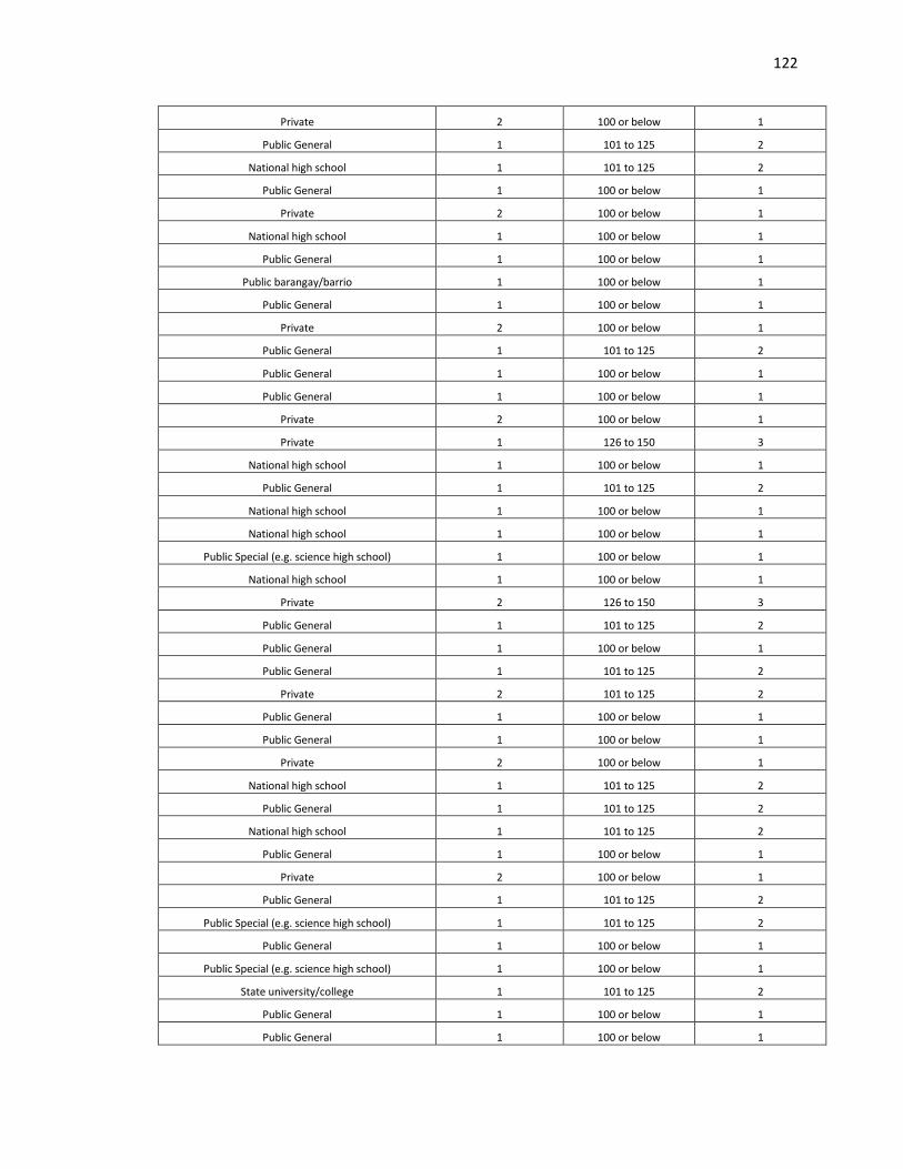
122
Private 2 100 or below 1
Public General 1 101 to 125 2
National high school 1 101 to 125 2
Public General 1 100 or below 1
Private 2 100 or below 1
National high school 1 100 or below 1
Public General 1 100 or below 1
Public barangay/barrio 1 100 or below 1
Public General 1 100 or below 1
Private 2 100 or below 1
Public General 1 101 to 125 2
Public General 1 100 or below 1
Public General 1 100 or below 1
Private 2 100 or below 1
Private 1 126 to 150 3
National high school 1 100 or below 1
Public General 1 101 to 125 2
National high school 1 100 or below 1
National high school 1 100 or below 1
Public Special (e.g. science high school) 1 100 or below 1
National high school 1 100 or below 1
Private 2 126 to 150 3
Public General 1 101 to 125 2
Public General 1 100 or below 1
Public General 1 101 to 125 2
Private 2 101 to 125 2
Public General 1 100 or below 1
Public General 1 100 or below 1
Private 2 100 or below 1
National high school 1 101 to 125 2
Public General 1 101 to 125 2
National high school 1 101 to 125 2
Public General 1 100 or below 1
Private 2 100 or below 1
Public General 1 101 to 125 2
Public Special (e.g. science high school) 1 101 to 125 2
Public General 1 100 or below 1
Public Special (e.g. science high school) 1 100 or below 1
State university/college 1 101 to 125 2
Public General 1 100 or below 1
Public General 1 100 or below 1

123
Public General 1 101 to 125 2
Private 2 101 to 125 2
Public General 1 101 to 125 2
Private 2 101 to 125 2
Private 2 100 or below 1
National high school 1 100 or below 1
Public General 1 100 or below 1
Private 2 100 or below 1
Public General 1 101 to 125 2
Private 2 100 or below 1
Private 2 101 to 125 2
Private 2 101 to 125 2
Private 2 100 or below 1
Public General 1 101 to 125 2
Private 2 100 or below 1
Public General 1 100 or below 1
Private 1 100 or below 1
Private 2 101 to 125 2
Private 2 100 or below 1
National high school 1 100 or below 1
Public General 1 100 or below 1
Public General 1 101 to 125 2
Private 2 101 to 125 2
Private 2 100 or below 1
Public General 1 101 to 125 2
Private 2 100 or below 1
National high school 1 100 or below 1
Public General 1 101 to 125 2
National high school 1 101 to 125 2
Private 2 101 to 125 2
Public Special (e.g. science high school) 1 100 or below 1
National high school 1 100 or below 1
National high school 1 101 to 125 2
Public General 1 100 or below 1
Public General 1 101 to 125 2
Public Special (e.g. science high school) 1 100 or below 1
afi
fa occu
P 7,001-P14,000 2 Employed as (Please specify the job) 3
P 7,001-P14,000 2 Employed as (Please specify the job) 3
P21,001-P28,000 4 Employed as (Please specify the job) 3

124
P 7,001-P14,000 2 Employed as (Please specify the job) 3
P14,001-P21,000 3 Self-Employed 2
P 7,001-P14,000 2 Employed as (Please specify the job) 3
P 7,001-P14,000 2 Employed as (Please specify the job) 3
P28,001-P35,000 5 Employed as (Please specify the job) 3
P14,001-P21,000 3 Unemployed 1
P 7,001-P14,000 2 Employed as (Please specify the job) 3
P14,001-P21,000 3 Unemployed 1
P21,001-P28,000 3 Employed as (Please specify the job) 3
P42,001-P49,000 5 Employed as (Please specify the job) 3
P 7,000 or below 1 Employed as (Please specify the job) 3
P 7,001-P14,000 2 Unemployed 1
P14,001-P21,000 3 Self-Employed 2
P28,001-P35,000 5 Employed as (Please specify the job) 3
P 7,001-P14,000 2 Employed as (Please specify the job) 3
P 7,001-P14,000 2 Employed as (Please specify the job) 3
P14,001-P21,000 3 Self-Employed 2
P14,001-P21,000 3 Employed as (Please specify the job) 3
P 7,000 or below 1 Employed as (Please specify the job) 3
P21,001-P28,000 4 Self-Employed 2
P14,001-P21,000 3 Employed as (Please specify the job) 3
P 7,001-P14,000 2 Unemployed 1
P14,001-P21,000 3 Employed as (Please specify the job) 3
P35,001-P42,000 5 Unemployed 1
P14,001-P21,000 3 Unemployed 1
P14,001-P21,000 3 Employed as (Please specify the job) 3
P 7,000 or below 1 Self-Employed 2
P21,001-P28,000 4 Employed as (Please specify the job) 3
P 7,000 or below 1 Employed as (Please specify the job) 3
P 7,001-P14,000 2 Employed as (Please specify the job) 3
P 7,001-P14,000 2 Employed as (Please specify the job) 3
P 7,000 or below 1 Employed as (Please specify the job) 3
P 7,000 or below 1 Unemployed 1
NULL 1 Self-Employed 2
P14,001-P21,000 3 Employed as (Please specify the job) 3
P 7,001-P14,000 2 Employed as (Please specify the job) 3
P49,001 or above 5 Employed as (Please specify the job) 3
P 7,001-P14,000 2 Employed as (Please specify the job) 3
P 7,001-P14,000 2 Employed as (Please specify the job) 3
P21,001-P28,000 4 Employed as (Please specify the job) 3
P49,001 or above 5 Self-Employed 2
P14,001-P21,000 3 Employed as (Please specify the job) 3

125
P28,001-P35,000 5 Employed as (Please specify the job) 3
P 7,000 or below 2 Employed as (Please specify the job) 3
P14,001-P21,000 3 Employed as (Please specify the job) 3
P14,001-P21,000 3 Unemployed 1
P 7,001-P14,000 2 Employed as (Please specify the job) 3
P 7,001-P14,000 2 Employed as (Please specify the job) 3
P 7,000 or below 1 Employed as (Please specify the job) 3
P21,001-P28,000 4 Self-Employed 2
P14,001-P21,000 3 Self-Employed 2
P14,001-P21,000 3 Employed as (Please specify the job) 3
P14,001-P21,000 3 Employed as (Please specify the job) 3
P 7,000 or below 1 Self-Employed 2
P14,001-P21,000 3 Unemployed 1
P 7,001-P14,000 2 Self-Employed 2
P 7,001-P14,000 2 Self-Employed 2
P21,001-P28,000 4 Employed as (Please specify the job) 3
P14,001-P21,000 3 Unemployed 1
P28,001-P35,000 5 Self-Employed 2
P 7,000 or below 1 Self-Employed 2
P14,001-P21,000 3 Employed as (Please specify the job) 3
P28,001-P35,000 5 Employed as (Please specify the job) 3
P21,001-P28,000 4 Employed as (Please specify the job) 3
P 7,000 or below 1 Employed as (Please specify the job) 3
P 7,000 or below 1 Employed as (Please specify the job) 3
P21,001-P28,000 4 Unemployed 1
P28,001-P35,000 5 Employed as (Please specify the job) 3
P14,001-P21,000 3 Employed as (Please specify the job) 3
P 7,001-P14,000 2 Employed as (Please specify the job) 3
P 7,000 or below 1 Self-Employed 2
P14,001-P21,000 3 Employed as (Please specify the job) 3
P 7,001-P14,000 2 Employed as (Please specify the job) 3
P42,001-P49,000 5 Employed as (Please specify the job) 3
P14,001-P21,000 3 Employed as (Please specify the job) 3
P 7,001-P14,000 2 Employed as (Please specify the job) 3
P14,001-P21,000 3 Employed as (Please specify the job) 3
P 7,000 or below 1 Self-Employed 2
P 7,001-P14,000 2 Unemployed 1
P 7,001-P14,000 2 Unemployed 1
P 7,001-P14,000 2 Self-Employed 2
P 7,001-P14,000 2 Employed as (Please specify the job) 3
P 7,001-P14,000 2 Employed as (Please specify the job) 3

126
P14,001-P21,000 3 Self-Employed 2
P 7,000 or below 1 Employed as (Please specify the job) 3
P 7,000 or below 1 Self-Employed 2
P 7,000 or below 1 Employed as (Please specify the job) 3
P 7,000 or below 1 Employed as (Please specify the job) 3
P28,001-P35,000 5 Self-Employed 2
P28,001-P35,000 5 Employed as (Please specify the job) 3
P 7,001-P14,000 2 Unemployed 1
P 7,001-P14,000 2 Employed as (Please specify the job) 3
P14,001-P21,000 3 Unemployed 1
P14,001-P21,000 3 Self-Employed 2
P14,001-P21,000 3 Self-Employed 2
P35,001-P42,000 5 Employed as (Please specify the job) 3
P 7,001-P14,000 2 Employed as (Please specify the job) 3
P 7,000 or below 1 Employed as (Please specify the job) 3
P 7,000 or below 1 Employed as (Please specify the job) 3
P14,001-P21,000 3 Self-Employed 2
P21,001-P28,000 4 Employed as (Please specify the job) 3
P14,001-P21,000 3 Unemployed 1
P14,001-P21,000 3 Employed as (Please specify the job) 3
P21,001-P28,000 4 Employed as (Please specify the job) 3
P 7,001-P14,000 2 Employed as (Please specify the job) 3
P 7,000 or below 1 Unemployed 1
P28,001-P35,000 5 Employed as (Please specify the job) 3
P14,001-P21,000 3 Self-Employed 2
P14,001-P21,000 3 Employed as (Please specify the job) 3
P 7,001-P14,000 2 Unemployed 1
P28,001-P35,000 5 Self-Employed 2
P14,001-P21,000 3 Unemployed 1
P28,001-P35,000 5 Employed as (Please specify the job) 3
P 7,001-P14,000 2 Self-Employed 2
P49,001 or above 5 Employed as (Please specify the job) 3
P14,001-P21,000 3 Self-Employed 2
P 7,000 or below 1 Unemployed 1
P 7,001-P14,000 2 Unemployed 1
P 7,000 or below 1 Employed as (Please specify the job) 3
P 7,001-P14,000 2 Employed as (Please specify the job) 3
P42,001-P49,000 5 Employed as (Please specify the job) 3
P14,001-P21,000 3 Unemployed 1
P14,001-P21,000 3 Employed as (Please specify the job) 3
P 7,000 or below 1 Employed as (Please specify the job) 3

127
P35,001-P42,000 5 Employed as (Please specify the job) 3
P49,001 or above 5 Employed as (Please specify the job) 3
P28,001-P35,000 5 Unemployed 1
P 7,001-P14,000 2 Self-Employed 2
P 7,001-P14,000 2 Unemployed 1
P21,001-P28,000 4 Employed as (Please specify the job) 3
P14,001-P21,000 3 Employed as (Please specify the job) 3
P 7,001-P14,000 2 Employed as (Please specify the job) 3
P49,001 or above 5 Unemployed 1
P42,001-P49,000 5 Employed as (Please specify the job) 3
P28,001-P35,000 5 Self-Employed 2
P14,001-P21,000 3 Employed as (Please specify the job) 3
P 7,001-P14,000 2 Employed as (Please specify the job) 3
P21,001-P28,000 4 Employed as (Please specify the job) 3
P14,001-P21,000 3 Self-Employed 2
fa educ
ma occu
ma educ
College Graduate 4 Employed as (Please specify the job) 3
College Undergraduate 4
College Graduate 4 Employed as (Please specify the job) 3
College Undergraduate 4
Voc/Tech Course Graduate 3 Employed as (Please specify the job) 3
College Graduate 4
High School Undergraduate 2 Employed as (Please specify the job) 3
College Undergraduate 7
High School Undergraduate 2 Employed as (Please specify the job) 3
Master’s Degree Graduate w/
units in a Doctorate program 5
College Undergraduate 4 Employed as (Please specify the job) 3
College Undergraduate 4
High School Graduate 2 Self-Employed 2
High School Graduate 4
College Graduate w/ units in Master’s program 5 Employed as (Please specify the job) 3
Master’s Degree Graduate 5
College Graduate 4 Unemployed 1
College Undergraduate 4
College Graduate 4 Employed as (Please specify the job) 3
High School Graduate 2
College Undergraduate 4 Unemployed 1
High School Graduate 2
College Undergraduate 4 Employed as (Please specify the job) 3
College Graduate 4
High School Undergraduate 2 Employed as (Please specify the job) 3
College Undergraduate 4
High School Graduate 2 Unemployed 1
Voc/Tech Undergraduate 3
College Undergraduate 4 Unemployed 1
Voc/Tech Undergraduate 3

128
College Graduate 4 Employed as (Please specify the job) 3
College Graduate 4
College Graduate 4 Employed as (Please specify the job) 3
College Undergraduate 4
High School Undergraduate 2 Unemployed 1
College Undergraduate 4
High School Undergraduate 2 Employed as (Please specify the job) 3
High School Undergraduate 2
College Graduate 4 Employed as (Please specify the job) 3
College Graduate 4
College Undergraduate 4 Employed as (Please specify the job) 3
College Graduate 4
Elementary Graduate 1 Unemployed 1
Elementary Graduate 1
High School Graduate 2 Unemployed 1
College Undergraduate 4
High School Undergraduate 2 Unemployed 1
High School Undergraduate 2
College Undergraduate 4 Self-Employed 2
High School Graduate 2
College Undergraduate 4 Employed as (Please specify the job) 3
High School Undergraduate 2
High School Graduate 2 Self-Employed 2
College Graduate 4
College Graduate 4 Employed as (Please specify the job) 3
College Graduate 4
Master’s Degree Graduate 5 Unemployed 1
College Undergraduate 4
High School Graduate 2 Unemployed 1
High School Graduate 2
College Graduate w/ units in Master’s program 5 Employed as (Please specify the job) 3
College Graduate 4
High School Undergraduate 2 Unemployed 1
High School Undergraduate 2
High School Graduate 2 Unemployed 1
High School Graduate 2
College Undergraduate 4 Employed as (Please specify the job) 3
College Graduate 4
College Graduate 4 Unemployed 1
College Graduate 4
Elementary Undergraduate 1 Unemployed 1
High School Undergraduate 2
High School Graduate 2 Self-Employed 2
High School Undergraduate 2
College Graduate 4 Employed as (Please specify the job) 3
College Graduate 4
High School Graduate 2 Employed as (Please specify the job) 3
College Graduate 4
College Graduate 4 Self-Employed 2
College Graduate 4
College Undergraduate 4 Unemployed 1
College Graduate 4
College Undergraduate 4 Unemployed 1
High School Graduate 2

129
High School Graduate 2 Employed as (Please specify the job) 3
College Graduate 4
College Graduate 4 Employed as (Please specify the job) 3
Doctorate Degree Holder 5
College Graduate 4 Self-Employed 2
High School Undergraduate 2
College Graduate w/ units in Master’s program 5 Unemployed 1
High School Undergraduate 2
College Undergraduate 4 Unemployed 1
High School Graduate 2
College Graduate 4 Unemployed 1
College Graduate 4
College Undergraduate 4 Employed as (Please specify the job) 3
College Graduate 4
High School Graduate 2 Employed as (Please specify the job) 3
High School Graduate 2
College Graduate 4 Employed as (Please specify the job) 3
College Graduate 4
High School Graduate 2 Unemployed 1
High School Graduate 2
High School Undergraduate 2 Employed as (Please specify the job) 3
College Graduate w/ units in
Master’s program 5
College Graduate 4 Self-Employed 2
High School Graduate 2
College Graduate 4 Self-Employed 2
High School Undergraduate 2
College Undergraduate 4 Self-Employed 2
College Graduate 4
High School Graduate 2 Unemployed 1
College Graduate 4
College Graduate 4 Self-Employed 2
College Graduate 4
High School Graduate 2 Employed as (Please specify the job) 3
College Graduate 4
College Undergraduate 4 Self-Employed 2
College Undergraduate 4
Voc/Tech Course Graduate 3 Self-Employed 2
High School Graduate 2
High School Undergraduate 2 Self-Employed 2
College Graduate 4
College Undergraduate 4 Unemployed 1
College Graduate 4
High School Undergraduate 2 Self-Employed 2
College Graduate 4
College Graduate 4 Employed as (Please specify the job) 3
College Graduate 4
College Undergraduate 4 Self-Employed 2
High School Undergraduate 2
College Graduate 4 Employed as (Please specify the job) 2
College Graduate 4
High School Undergraduate 3 Employed as (Please specify the job) 2
High School Graduate 2
High School Graduate 2 Unemployed 1
High School Graduate 2

130
College Undergraduate 4 Unemployed 1
College Undergraduate 4
College Undergraduate 4 Unemployed 1
High School Graduate 2
College Graduate 4 Unemployed 1
High School Graduate 2
High School Undergraduate 2 Unemployed 1
High School Graduate 2
College Undergraduate 4 Unemployed 1
College Undergraduate 4
College Undergraduate 4 Unemployed 1
Voc/Tech Undergraduate 3
High School Undergraduate 2 Employed as (Please specify the job) 3
High School Graduate 2
Elementary Graduate 1 Unemployed 1
Elementary Graduate 1
College Undergraduate 4 Unemployed 1
College Undergraduate 4
High School Graduate 2 Employed as (Please specify the job) 3
High School Graduate 2
College Graduate 4 Employed as (Please specify the job) 3
College Graduate 4
Voc/Tech Course Graduate 3 Unemployed 1
High School Graduate 2
College Undergraduate 4 Employed as (Please specify the job) 3
College Graduate 4
College Undergraduate 4 Unemployed 1
High School Graduate 2
High School Undergraduate 2 Self-Employed 2
College Undergraduate 4
Voc/Tech Undergraduate 3 Unemployed 1
College Undergraduate 4
College Graduate 4 Self-Employed 2
College Graduate 4
College Graduate 4 Unemployed 1
College Graduate 4
Elementary Undergraduate 1 Unemployed 1
High School Undergraduate 2
Elementary Graduate 1 Self-Employed 2
High School Undergraduate 2
College Graduate 4 Unemployed 1
Elementary Graduate 1
High School Graduate 2 Self-Employed 2
College Undergraduate 4
Elementary Undergraduate 1 Self-Employed 2
High School Graduate 2
College Undergraduate 4 Unemployed 1
College Graduate 4
Elementary Graduate 1 Unemployed 1
Elementary Graduate 1
Voc/Tech Course Graduate 3 Unemployed 1
High School Graduate 2
College Undergraduate 4 Unemployed 1
High School Graduate 2

131
College Undergraduate 4 Unemployed 1
College Undergraduate 4
High School Undergraduate 2 Self-Employed 2
Voc/Tech Course Graduate 3
College Graduate w/ units in Master’s program 5 Employed as (Please specify the job) 3
Doctorate Degree Holder 5
High School Graduate 2 Self-Employed 2
High School Graduate 2
Voc/Tech Undergraduate 3 Unemployed 1
Voc/Tech Undergraduate 3
College Undergraduate 4 Unemployed 1
High School Graduate 2
College Undergraduate 4 Self-Employed 2
College Graduate 4
College Undergraduate 4 Employed as (Please specify the job) 3
College Graduate 4
High School Graduate 2 Employed as (Please specify the job) 3
College Undergraduate 4
High School Undergraduate 2 Self-Employed 2
High School Undergraduate 2
College Undergraduate 4 Self-Employed 2
College Graduate 4
College Undergraduate 4 Unemployed 1
College Undergraduate 4
Elementary Undergraduate 1 Unemployed 1
Elementary Undergraduate 1
College Graduate 4 Unemployed 1
College Graduate 4
College Graduate w/ units in Master’s program 5 Unemployed 1
College Graduate w/ units in
Master’s program 5
College Graduate w/ units in Master’s program 5 Unemployed 1
College Graduate w/ units in
Master’s program 5
High School Graduate 2 Employed as (Please specify the job) 3
College Graduate 4
College Undergraduate 4 Unemployed 1
College Undergraduate 4
College Undergraduate 4 Employed as (Please specify the job) 3
College Graduate 4
College Graduate 4 Employed as (Please specify the job) 3
College Undergraduate 4
High School Graduate 2 Unemployed 1
College Undergraduate 4
College Undergraduate 4 Employed as (Please specify the job) 3
College Graduate 4
College Graduate 4 Unemployed 1
High School Graduate 2
College Graduate 4 Unemployed 1
College Undergraduate 4
College Undergraduate 4 Employed as (Please specify the job) 3
College Undergraduate 4
College Graduate 4 Unemployed 1
College Undergraduate 4

132
College Undergraduate 4 Unemployed 1
College Undergraduate 4
College Graduate 4 Unemployed 1
College Graduate 4
College Graduate 4 Employed as (Please specify the job) 3
College Graduate 4
High School Graduate 2 Unemployed 1
High School Graduate 2
College Graduate 4 Unemployed 1
College Undergraduate 4
College Graduate 4 Unemployed 1
College Graduate 4
College Graduate w/ units in Master’s program 5 Employed as (Please specify the job) 3
College Graduate w/ units in
Master’s program 5
College Graduate 4 Employed as (Please specify the job) 3
College Graduate 4
College Undergraduate 4 Unemployed 1
High School Graduate 2
High School Graduate 2 Unemployed 1
College Undergraduate 4
College Graduate 4 Self-Employed 2
College Graduate 4
College Undergraduate 4 Unemployed 1
College Undergraduate 4
College Graduate 4 Employed as (Please specify the job) 3
High School Graduate 4
College Graduate 4 Self-Employed 3
Voc/Tech Course Graduate 3
College Graduate w/ units in Master’s program 5 Unemployed 1
College Graduate 4
College Graduate 4 Unemployed 1
High School Undergraduate 2
College Graduate 4 Employed as (Please specify the job) 3
College Graduate 4
High School Graduate 4 Self-Employed 2
High School Graduate 2
College Graduate 4 Self-Employed 2
College Graduate 4
College Graduate w/ units in Master’s 5 Employed as (Please specify the job) 3
College Graduate w/ units in
Master’s program 5
A.Y. 2011 – 2012
SectCode CourseCode coding SG coding AFI
1 BSPE 2 Private 2 P 7,000 or below 1
2 BSE 1 Private 2 P 7,001-P14,000 2
1 BSE 1 Public vocational 1
P 7,001-P14,000 2
1 BSE 1 Public vocational 1
P 7,001-P14,000

133
2 BSE 1 State university/college 1
P49,001 or above 5
1 BSE 1 Private 2 P 7,001-P14,000 2
1 BSE 1 Private 2 P21,001-P28,000 4
2 BSE 1 Public General 1 P 7,000 or below 1
1 BSPE 2 Private 2 P49,001 or above 5
2 BSE 1 National high school 1 P28,001-P35,000 5
1 BSE 1 Private 2
P28,001-P35,000 5
1 BSE 1 Public General 1
P 7,001-P14,000 2
1 BSE 1 Private 2
P14,001-P21,000 3
2 BSE 1 Private 2 P35,001-P42,000 5
2 BSE 1 Private 2 P 7,000 or below 1
2 BSE 1 National high school 1 P14,001-P21,000 3
1 BSE 1 Private 2 P21,001-P28,000 4
1 BSE 1 Private 2 P 7,000 or below 1
1 BSPE 2 Private 2
P 7,001-P14,000 2
1 BSE 1 Private 2
P14,001-P21,000 3
1 BSPE 2 Public General 1
P28,001-P35,000 5
2 BSE 1 Private 2 P35,001-P42,000 5
1 BSE 1 Public General 1 P 7,000 or below 1
1 BSPE 2 National high school 1 P 7,000 or below 1
2 BSE 1 Private 2 P28,001-P35,000 5
2 BSE 1 Private 2 P 7,001-P14,000 2
1 BSPE 2 National high school 1 P 7,001-P14,000 2
2 BSE 1 National high school 1
P 7,001-P14,000 2
1 BSE 1 Private 2
P14,001-P21,000 3
1 BSE 1 Private 2
P35,001-P42,000 5
1 BSPE 2 Public barangay/barrio 1 P21,001-P28,000 4
2 BSE 1 Private 2 P 7,001-P14,000 2
1 BSPE 2 Public General 1 P14,001-P21,000 3
1 BSPE 2 Public Special (e.g. science high school) 1 P14,001-P21,000 3
1 BSPE 2 Public General 1 P28,001-P35,000 5

134
1 BSPE 2 Public General 1
P14,001-P21,000 3
1 BSPE 2 Public barangay/barrio 1 P 7,000 or below 1
2 BSE 1 Private 2 P21,001-P28,000 4
1 BSPE 2 Private 2 P14,001-P21,000 3
1 BSPE 2 National high school 1 P28,001-P35,000 5
1 BSE 1 Private 2 P28,001-P35,000 5
1 BSE 1 Private 2
P28,001-P35,000 5
1 BSPE 2 Public General 1
P 7,001-P14,000 2
1 BSPE 2 Public General 1
P 7,001-P14,000 2
1 BSE 1 Private 2 P21,001-P28,000 4
1 BSE 1 Public General 1 P 7,001-P14,000 2
1 BSPE 2 Private 2 P14,001-P21,000 3
2 BSE 1 Private 2 P 7,001-P14,000 2
1 BSPE 2 National high school 1 P 7,000 or below 1
1 BSE 1 Public Special (e.g. science high school) 1
P14,001-P21,000 3
1 BSE 1 Public General 1
P14,001-P21,000 3
2 BSE 1 National high school 1
P 7,000 or below 1
1 BSE 1 Private 2 P 7,001-P14,000 2
1 BSPE 2 Public General 1 P 7,000 or below 1
2 BSE 1 Public barangay/barrio 1 P28,001-P35,000 5
1 BSE 1 Private 2 P 7,000 or below 1
1 BSPE 2 Public General 1 P 7,000 or below 1
1 BSPE 2 National high school 1 P 7,001-P14,000 2
2 BSE 1 Private 2
P14,001-P21,000 3
1 BSPE 2 Public General 1
P14,001-P21,000 3
1 BSPE 2 Private 2
P14,001-P21,000 3
1 BSE 1 Private 2 P28,001-P35,000 5
2 BSE 1 Public General 1 P14,001-P21,000 3
1 BSE 1 Public General 1 P 7,001-P14,000 2
1 BSPE 2 National high school 1 P14,001-P21,000 3
1 BSE 1 Private 2 P21,001-P28,000 4

135
2 BSE 1 Private 2
P14,001-P21,000 3
2 BSE 1 Public General 1 P 7,001-P14,000 2
1 BSPE 2 Private 2 P 7,001-P14,000 2
1 BSPE 2 Public General 1 P 7,001-P14,000 2
2 BSE 1 Public General 1 P 7,001-P14,000 2
1 BSE 1 Public General 1 P 7,001-P14,000 2
1 BSE 1 Private 2
P 7,000 or below 1
1 BSE 1 Public General 1
P14,001-P21,000 3
1 BSPE 2 Public General 1
P 7,000 or below 1
1 BSE 1 Private 2 P 7,001-P14,000 2
1 BSE 1 Public General 1 P 7,001-P14,000 2
1 BSPE 2 National high school 1 P28,001-P35,000 5
1 BSE 1 Public General 1 P21,001-P28,000 4
1 BSPE 2 Private 2 P 7,000 or below 1
2 BSE 1 National high school 1
P 7,001-P14,000 2
2 BSE 1 Public General 2
P 7,001-P14,000 2
2 BSE 1 Public Special (e.g. science high school) 1
P14,001-P21,000 3
1 BSPE 2 Private 2 P21,001-P28,000 4
1 BSE 1 Public Special (e.g. science high school) 1 P14,001-P21,000 3
PUPCET
H S A
GWA
moeduc
100 or below 1 88.01 to 90 5 2
High School Graduate 2
101 to 125 2 86.01 to 88 4 1.75
College Graduate 4
100 or below 1 88.01 to 90 5 1.833333
High School Graduate 2
100 or below 1 90.01 to 92 6 1.833333
High School Graduate 2
100 or below 1 84.01 to 86 3 1.416667
College Undergraduate 4
100 or below 1 90.01 to 92 6 1.916667
College Graduate 4
100 or below 1 86.01 to 88 4 1.75
College Graduate 4
101 to 125 2 88.01 to 90 5 1.5
High School Graduate 2
101 to 125 2 94.01 to 96 8 1.375
College Graduate 4

136
100 or below 1 88.01 to 90 5 1.75
College Graduate 4
101 to 125 2 90.01 to 92 6 1.833333
College Graduate 4
101 to 125 2 88.01 to 90 5 1.916667
High School Undergraduate 2
101 to 125 2 88.01 to 90 5 2.083333
College Undergraduate 4
100 or below 1 90.01 to 92 6 2
College Graduate 4
100 or below 1 84.01 to 86 3 2.083333
College Graduate 4
100 or below 1 88.01 to 90 5 1.875
Voc/Tech Undergraduate 3
126 to 150 3 86.01 to 88 4 1.916667
College Graduate 4
100 or below 1 88.01 to 90 5 1.916667
College Graduate 4
101 to 125 2 86.01 to 88 4 1.75
College Undergraduate 4
101 to 125 2 92.01 to 94 7 1.75
College Undergraduate 4
101 to 125 2 90.01 to 92 6 1.875
College Graduate w/ units in
Master’s program 5
100 or below 1 86.01 to 88 4 1.583333
College Graduate 4
101 to 125 2 88.01 to 90 5 1.666667
Elementary Undergraduate 1
101 to 125 2 84.01 to 86 3 1.5
College Graduate 4
100 or below 1 88.01 to 90 5 2.166667
College Undergraduate 4
126 to 150 3 90.01 to 92 6 1.416667
College Graduate 4
101 to 125 2 86.01 to 88 4 1.5
High School Graduate 4
101 to 125 2 82.01 to 84 2 2.25
High School Undergraduate 2
101 to 125 2 88.01 to 90 5 2
College Graduate w/ units in
Master’s program 5
100 or below 1 86.01 to 88 4 1.916667
College Graduate 4
100 or below 1 86.01 to 88 4 1.375
College Graduate 4
100 or below 1 90.01 to 92 6 1.916667
High School Undergraduate 2
100 or below 1 86.01 to 88 4 1.5
College Graduate 4
101 to 125 2 90.01 to 92 6 1.75
College Graduate 4
1 90.01 to 92 6 1.625
College Graduate 4
100 or below 1 86.01 to 88 4 1.875
College Undergraduate 4
100 or below 1 86.01 to 88 4 2
High School Graduate 2

137
101 to 125 2 84.01 to 86 3 1.916667
College Undergraduate 4
100 or below 1 86.01 to 88 4 1.5
College Graduate 4
100 or below 1 92.01 to 94 6 1.75
College Graduate 4
100 or below 1 86.01 to 88 4 1.75
Master’s Degree Graduate
w/ units in a Doctorate
program 5
101 to 125 2 88.01 to 90 5 1.583333
College Graduate 4
101 to 125 2 88.01 to 90 5 1.5
High School Undergraduate 2
100 or below 1 84.01 to 86 3 1.75
Elementary Graduate 1
101 to 125 2 88.01 to 90 5 1.916667
Voc/Tech Course Graduate 3
100 or below 1 92.01 to 94 6 1.916667
High School Graduate 2
101 to 125 2 88.01 to 90 5 1.5
College Graduate 4
100 or below 1 88.01 to 90 5 1.916667
College Graduate 4
I am a PUPLHS graduate / I took PUPSAIT / I am an Entrance Scholar 1 92.01 to 94 6 1.5
High School Undergraduate 2
101 to 125 2 88.01 to 90 5 1.833333
College Undergraduate 4
101 to 125 2 92.01 to 94 7 1.833333
College Undergraduate 4
100 or below 1 86.01 to 88 4 1.833333
Elementary Graduate 1
101 to 125 2 90.01 to 92 6 1.75
Voc/Tech Course Graduate 3
101 to 125 2 86.01 to 88 4 1.875
Elementary Graduate 2
100 or below 1 82.01 to 84 2 1.916667
College Graduate 4
101 to 125 2 86.01 to 88 4 1.916667
Elementary Undergraduate 1
101 to 125 2 82.01 to 84 2 1.625
High School Graduate 2
101 to 125 2 88.01 to 90 5 1.5
High School Graduate 2
101 to 125 2 88.01 to 90 5 1.75
Voc/Tech Course Graduate 3
I am a PUPLHS graduate / I took PUPSAIT / I am an Entrance Scholar 1 90.01 to 92 6 1.625
Voc/Tech Course Graduate 3
100 or below 1 84.01 to 86 3 2
Master’s Degree Graduate 5
100 or below 1 88.01 to 90 5 1.916667
College Graduate w/ units in
Master’s program 5
100 or below 1 88.01 to 90 5 2.5
College Undergraduate 4
101 to 125 2 86.01 to 88 4 2.083333
High School Undergraduate 2
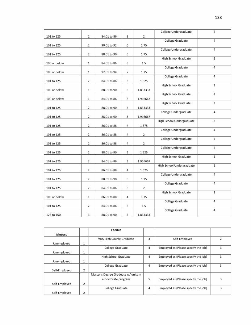
138
101 to 125 2 84.01 to 86 3 2
College Undergraduate 4
101 to 125 2 90.01 to 92 6 1.75
College Graduate 4
101 to 125 2 88.01 to 90 5 1.75
College Undergraduate 4
100 or below 1 84.01 to 86 3 1.5
High School Graduate 2
100 or below 1 92.01 to 94 7 1.75
College Graduate 4
101 to 125 2 84.01 to 86 3 1.625
College Graduate 4
100 or below 1 88.01 to 90 5 1.833333
High School Graduate 2
100 or below 1 84.01 to 86 3 1.916667
High School Graduate 2
101 to 125 2 88.01 to 90 5 1.833333
High School Graduate 2
101 to 125 2 88.01 to 90 5 1.916667
College Undergraduate 4
101 to 125 2 86.01 to 88 4 1.875
High School Undergraduate 2
101 to 125 2 86.01 to 88 4 2
College Undergraduate 4
101 to 125 2 86.01 to 88 4 2
College Undergraduate 4
101 to 125 2 88.01 to 90 5 1.625
College Undergraduate 4
101 to 125 2 84.01 to 86 3 1.916667
High School Graduate 2
101 to 125 2 86.01 to 88 4 1.625
High School Undergraduate 2
101 to 125 2 88.01 to 90 5 1.75
College Undergraduate 4
101 to 125 2 84.01 to 86 3 2
College Graduate 4
100 or below 1 86.01 to 88 4 1.75
High School Graduate 2
101 to 125 2 84.01 to 86 3 1.5
College Graduate 4
126 to 150 3 88.01 to 90 5 1.833333
College Graduate 4
Mooccu
Faeduc
Unemployed 1
Voc/Tech Course Graduate 3 Self-Employed 2
Unemployed 1
College Graduate 4 Employed as (Please specify the job) 3
Unemployed 1
High School Graduate 4 Employed as (Please specify the job) 3
Self-Employed 2
College Graduate 4 Employed as (Please specify the job) 3
Self-Employed 2
Master’s Degree Graduate w/ units in
a Doctorate program 5 Employed as (Please specify the job) 3
Self-Employed 2
College Graduate 4 Employed as (Please specify the job) 3

139
Employed as (Please specify the job) 3
High School Graduate 2 Employed as (Please specify the job) 3
Unemployed 1
Elementary Undergraduate 1 Self-Employed 2
Employed as (Please specify the job) 3
College Graduate 4 Employed as (Please specify the job) 3
Unemployed 1
High School Graduate 2 Self-Employed 2
Unemployed 1
College Graduate 4 Employed as (Please specify the job) 3
Unemployed 3
High School Undergraduate 2 Self-Employed 2
Employed as (Please specify the job) 3
High School Graduate 2 Self-Employed 2
Employed as (Please specify the job) 3
High School Graduate 2 Self-Employed 2
Unemployed 1
High School Graduate 2 Unemployed 1
Unemployed 1
College Undergraduate 4 Employed as (Please specify the job) 3
Unemployed 1
College Graduate 4 Unemployed 1
Unemployed 1
College Graduate 4 Employed as (Please specify the job) 3
Employed as (Please specify the job) 3
Voc/Tech Course Graduate 3 Self-Employed 2
Unemployed 1
College Graduate 4 Employed as (Please specify the job) 3
Employed as (Please specify the job) 3
College Graduate 4 Employed as (Please specify the job) 3
Unemployed 1
College Graduate 4 Unemployed 1
Employed as (Please specify the job) 3
High School Undergraduate 2 Employed as (Please specify the job) 3
Self-Employed 2
College Graduate 4 Employed as (Please specify the job) 3
Unemployed 1
College Graduate 4 Unemployed 1
Self-Employed 2
Voc/Tech Course Graduate 3 Self-Employed 2
Unemployed 1
High School Graduate 2 Employed as (Please specify the job) 3
Unemployed 1
High School Graduate 2 Employed as (Please specify the job) 3
Employed as (Please specify the job) 3
College Graduate w/ units in
Master’s program 5 Unemployed 1
Employed as (Please specify the job) 3
College Graduate 4 Employed as (Please specify the job) 3
Employed as (Please specify the job) 3
High School Graduate 2 Self-Employed 2
Unemployed 1
College Undergraduate 4 Self-Employed 2
Employed as (Please specify the job) 3
Voc/Tech Undergraduate 3 Self-Employed 2
Self-Employed 2
College Graduate 4 Employed as (Please specify the job) 3
Employed as (Please specify the job) 3
College Graduate 4 Employed as (Please specify the job) 3

140
Unemployed 1
College Undergraduate 4 Employed as (Please specify the job) 3
Self-Employed 2
College Undergraduate 4 Self-Employed 2
Self-Employed 2
College Graduate 4 Employed as (Please specify the job) 3
Self-Employed 2
College Undergraduate 4 Self-Employed 2
Unemployed 1
College Undergraduate 4 Employed as (Please specify the job) 3
Employed as (Please specify the job) 3
High School Graduate 2 Self-Employed 2
Employed as (Please specify the job) 3
College Graduate 4 Employed as (Please specify the job) 3
Unemployed 1
College Graduate 4 Employed as (Please specify the job) 3
Unemployed 1
College Graduate 4 Employed as (Please specify the job) 3
Employed as (Please specify the job) 3
College Undergraduate 4 Employed as (Please specify the job) 3
Unemployed 1
High School Graduate 2 Employed as (Please specify the job) 3
Unemployed 1
College Graduate 4 Employed as (Please specify the job) 3
Employed as (Please specify the job) 3
College Graduate 4 Employed as (Please specify the job) 3
Unemployed 1
College Graduate 4 Unemployed 1
Unemployed 1
High School Undergraduate 2 Self-Employed 2
Employed as (Please specify the job) 3
College Undergraduate 4 Employed as (Please specify the job) 3
Unemployed 1
High School Graduate 2 Employed as (Please specify the job) 3
Unemployed 1
College Graduate 4 Self-Employed 2
Employed as (Please specify the job) 3
High School Graduate 2 Self-Employed 2
Employed as (Please specify the job) 3
Elementary Undergraduate 1 Unemployed 1
Self-Employed 2
Elementary Undergraduate 1 Self-Employed 2
Self-Employed 2
Voc/Tech Course Graduate 3 Employed as (Please specify the job) 3
Unemployed 1
College Graduate 4 Unemployed 1
Unemployed 1
Voc/Tech Course Graduate 3 Self-Employed 2
Unemployed 1
Master’s Degree Graduate 5 Employed as (Please specify the job) 3
Self-Employed 2
Voc/Tech Course Graduate 3 Self-Employed 2
Self-Employed 2
College Undergraduate 4 Self-Employed 2
Employed as (Please specify the job) 3
College Graduate 4 Employed as (Please specify the job) 3
Unemployed 1
Voc/Tech Course Graduate 3 Self-Employed 2

141
Employed as (Please specify the job) 3
High School Undergraduate 2 Employed as (Please specify the job) 3
Employed as (Please specify the job) 3
High School Undergraduate 2 Self-Employed 2
Unemployed 1
College Undergraduate 4 Employed as (Please specify the job) 3
Unemployed 1
Voc/Tech Undergraduate 3 Employed as (Please specify the job) 3
Unemployed 1
College Graduate 4 Employed as (Please specify the job) 3
Unemployed 1
College Graduate 4 Unemployed 1
Unemployed 1
College Graduate 4 Employed as (Please specify the job) 3
Unemployed 1
High School Graduate 2 Employed as (Please specify the job) 3
Unemployed 1
High School Graduate 2 Employed as (Please specify the job) 3
Unemployed 1
College Graduate 4 Employed as (Please specify the job) 3
Unemployed 1
Elementary Undergraduate 1 Unemployed 1
Unemployed 1
College Undergraduate 4 Employed as (Please specify the job) 3
Unemployed 1
College Undergraduate 4 Employed as (Please specify the job) 3
Unemployed 1
Voc/Tech Undergraduate 3 Employed as (Please specify the job) 3
Employed as (Please specify the job) 3
High School Graduate 2 Unemployed 1
Self-Employed 2
High School Undergraduate 1 Unemployed 1
Unemployed 1
Voc/Tech Course Graduate 3 Employed as (Please specify the job) 3
Self-Employed 2
College Graduate 4 Employed as (Please specify the job) 3
Unemployed 1
Voc/Tech Course Graduate 3 Employed as (Please specify the job) 3
Employed as (Please specify the job) 3
College Graduate 4 Employed as (Please specify the job) 3
Self-Employed 2
College Undergraduate 4 Employed as (Please specify the job) 3

142
APPENDIX B
2009 – 2010
CSC
Frequency Percent Valid Percent
Cumulative
Percent
Valid BSE 72 75.8 75.8 75.8
BSPE 23 24.2 24.2 100.0
Total 95 100.0 100.0
HAS
Frequency Percent Valid Percent
Cumulative
Percent
Valid 82 - below 2 2.1 2.1 2.1
82.01 - 84 1 1.1 1.1 3.2
84.01 - 86 15 15.8 15.8 18.9
86.01 - 88 25 26.3 26.3 45.3
88.01 - 90 32 33.7 33.7 78.9
90.01 - above 20 21.1 21.1 100.0
Total 95 100.0 100.0
SG
Frequency Percent Valid Percent
Cumulative
Percent
Valid Public 58 61.1 61.1 61.1
Private 37 38.9 38.9 100.0
Total 95 100.0 100.0
PS
Frequency Percent Valid Percent
Cumulative
Percent

143
Valid 100 - below 43 45.3 45.3 45.3
101 - 125 43 45.3 45.3 90.5
126 - above 9 9.5 9.5 100.0
Total 95 100.0 100.0
AFI
Frequency Percent Valid Percent
Cumulative
Percent
Valid 7,000 and below 16 16.8 16.8 16.8
7,001 - 14,000 19 20.0 20.0 36.8
14,001 - 21,000 27 28.4 28.4 65.3
21,001 - 28,000 5 5.3 5.3 70.5
28,001 - above 28 29.5 29.5 100.0
Total 95 100.0 100.0
Faoccu
Frequency Percent Valid Percent
Cumulative
Percent
Valid unemployed 12 12.6 12.6 12.6
self-employed 27 28.4 28.4 41.1
employed 56 58.9 58.9 100.0
Total 95 100.0 100.0
Maoccu
Frequency Percent Valid Percent
Cumulative
Percent
Valid unemployed 47 49.5 49.5 49.5
self-employed 23 24.2 24.2 73.7
employed 25 26.3 26.3 100.0
Total 95 100.0 100.0

144
moeduc
Frequency Percent Valid Percent
Cumulative
Percent
Valid elem. undergrad. elem. grad 9 9.5 9.5 9.5
hs undergrad/ hs grad 27 28.4 28.4 37.9
voc/tech undergrad,
voc/tech grad
5 5.3 5.3 43.2
coll. undergrad, coll. grad 52 54.7 54.7 97.9
coll. gard w/ units in
master's, master's, master's
grad w/ units in doct.,
doctorate
2 2.1 2.1 100.0
Total 95 100.0 100.0
faeduc
Frequency Percent Valid Percent
Cumulative
Percent
Valid elem. undergrad/elem. grad 6 6.3 6.3 6.3
hs undergrad/hs grad 33 34.7 34.7 41.1
voc/tech undergrad,
voc/tech grad
7 7.4 7.4 48.4
coll. undergrad/coll. grad 44 46.3 46.3 94.7
coll. grad w/ units in
master's, master's, master's
grad w/ units in doct.,
doctorate
5 5.3 5.3 100.0
Total 95 100.0 100.0
Group Statistics
CSC N Mean Std. Deviation Std. Error Mean
GWA BSE 72 2.0577 .26907 .03171
BSPE 23 2.0304 .16655 .03473

145
Independent Samples Test
Levene's Test for
Equality of Variances t-test for Equality of Means
F Sig. t Df
Sig. (2-
tailed)
Mean
Difference
Std. Error
Difference
95% Confidence
Interval of the
Difference
Lower Upper
GW
A
Equal variances
assumed
9.680 .002 .458 93 .648 .02729 .05956 -.09099 .14556
Equal variances
not assumed
.580 60.86
8
.564 .02729 .04703 -.06676 .12133
Group Statistics
SG N Mean Std. Deviation Std. Error Mean
GWA Public 58 2.0683 .24771 .03253
Private 37 2.0241 .24844 .04084
Independent Samples Test
Levene's Test for
Equality of Variances t-test for Equality of Means
F Sig. t df
Sig. (2-
tailed)
Mean
Difference
Std. Error
Difference
95% Confidence
Interval of the
Difference
Lower Upper
G
W
A
Equal variances
assumed
.144 .705 .847 93 .399 .04417 .05218 -.05944 .14779
Equal variances not
assumed
.846 76.667 .400 .04417 .05221 -.05980 .14815

146
ANOVA
GWA
Sum of Squares Df Mean Square F Sig.
Between Groups 1.169 5 .234 4.530 .001
Within Groups 4.594 89 .052
Total 5.764 94
ANOVA
GWA
Sum of Squares Df Mean Square F Sig.
Between Groups .186 4 .047 .752 .560
Within Groups 5.577 90 .062
Total 5.764 94
ANOVA
GWA
Sum of Squares Df Mean Square F Sig.
Between Groups .057 2 .028 .457 .635
Within Groups 5.707 92 .062
Total 5.764 94
ANOVA
GWA
Sum of Squares Df Mean Square F Sig.
Between Groups .093 2 .047 .758 .471
Within Groups 5.670 92 .062
Total 5.764 94

147
ANOVA
GWA
Sum of Squares Df Mean Square F Sig.
Between Groups .374 4 .093 1.560 .192
Within Groups 5.390 90 .060
Total 5.764 94
ANOVA
GWA
Sum of Squares Df Mean Square F Sig.
Between Groups .378 4 .094 1.577 .187
Within Groups 5.386 90 .060
Total 5.764 94
Correlations
GWA CSC HSA SG PS AFI
GWA Pearson Correlation 1 -.047 -.435** -.087 -.179 -.106
Sig. (2-tailed) .648 .000 .399 .083 .305
N 95 95 95 95 95 95
CSC Pearson Correlation -.047 1 .068 .053 -.181 -.075
Sig. (2-tailed) .648 .515 .613 .079 .470
N 95 95 95 95 95 95
HSA Pearson Correlation -.435** .068 1 .206
* .221
* .018
Sig. (2-tailed) .000 .515 .045 .031 .862
N 95 95 95 95 95 95
SG Pearson Correlation -.087 .053 .206* 1 .075 .091
Sig. (2-tailed) .399 .613 .045 .472 .380
N 95 95 95 95 95 95
PS Pearson Correlation -.179 -.181 .221* .075 1 .040
Sig. (2-tailed) .083 .079 .031 .472 .699
N 95 95 95 95 95 95

148
AFI Pearson Correlation -.106 -.075 .018 .091 .040 1
Sig. (2-tailed) .305 .470 .862 .380 .699
N 95 95 95 95 95 95
**. Correlation is significant at the 0.01 level (2-tailed).
*. Correlation is significant at the 0.05 level (2-tailed).
Correlations
GWA faoccu maoccu faeduc moeduc
GWA Pearson Correlation 1 -.090 .115 -.018 .169
Sig. (2-tailed) .386 .267 .864 .101
N 95 95 95 95 95
faoccu Pearson Correlation -.090 1 .003 .156 .038
Sig. (2-tailed) .386 .974 .130 .714
N 95 95 95 95 95
maoccu Pearson Correlation .115 .003 1 .090 .394**
Sig. (2-tailed) .267 .974 .385 .000
N 95 95 95 95 95
faeduc Pearson Correlation -.018 .156 .090 1 .347**
Sig. (2-tailed) .864 .130 .385 .001
N 95 95 95 95 95
moeduc Pearson Correlation .169 .038 .394** .347
** 1
Sig. (2-tailed) .101 .714 .000 .001
N 95 95 95 95 95
**. Correlation is significant at the 0.01 level (2-tailed).
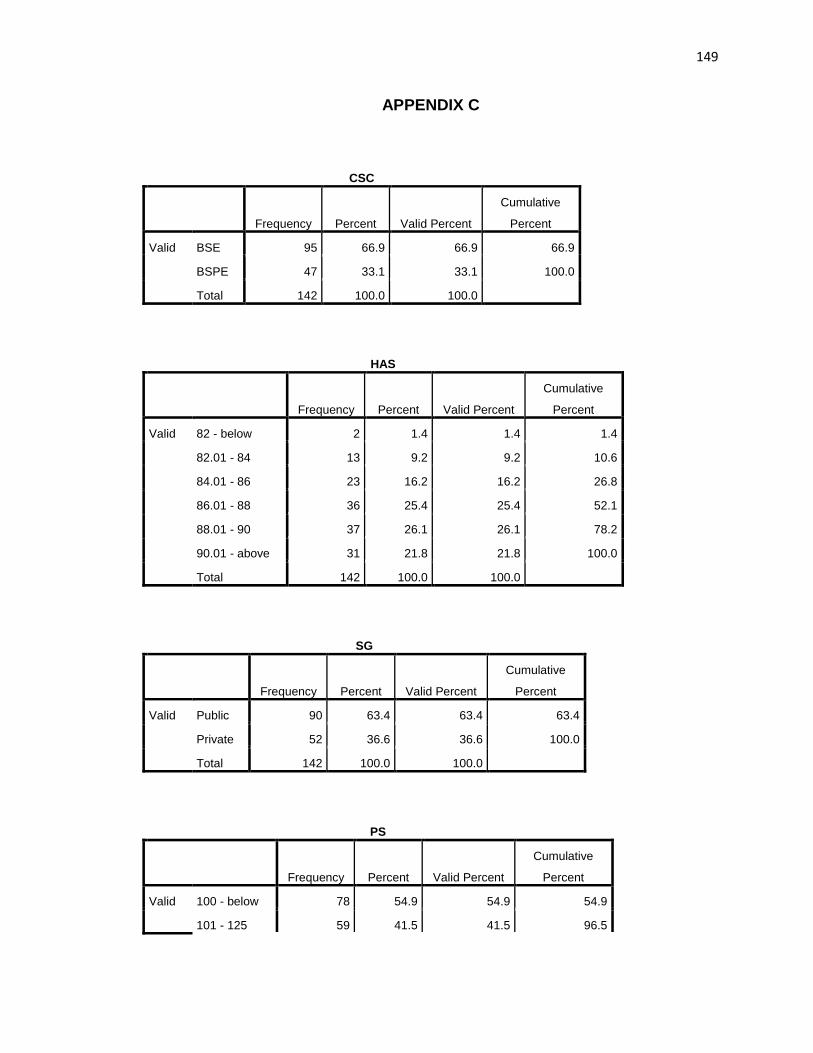
149
APPENDIX C
CSC
Frequency Percent Valid Percent
Cumulative
Percent
Valid BSE 95 66.9 66.9 66.9
BSPE 47 33.1 33.1 100.0
Total 142 100.0 100.0
HAS
Frequency Percent Valid Percent
Cumulative
Percent
Valid 82 - below 2 1.4 1.4 1.4
82.01 - 84 13 9.2 9.2 10.6
84.01 - 86 23 16.2 16.2 26.8
86.01 - 88 36 25.4 25.4 52.1
88.01 - 90 37 26.1 26.1 78.2
90.01 - above 31 21.8 21.8 100.0
Total 142 100.0 100.0
SG
Frequency Percent Valid Percent
Cumulative
Percent
Valid Public 90 63.4 63.4 63.4
Private 52 36.6 36.6 100.0
Total 142 100.0 100.0
PS
Frequency Percent Valid Percent
Cumulative
Percent
Valid 100 - below 78 54.9 54.9 54.9
101 - 125 59 41.5 41.5 96.5

150
126 - above 5 3.5 3.5 100.0
Total 142 100.0 100.0
AFI
Frequency Percent Valid Percent
Cumulative
Percent
Valid 7,000 and below 24 16.9 16.9 16.9
7,001 - 14,000 40 28.2 28.2 45.1
14,001 - 21,000 41 28.9 28.9 73.9
21,001 - 28,000 12 8.5 8.5 82.4
28,001 - above 25 17.6 17.6 100.0
Total 142 100.0 100.0
faoccu
Frequency Percent Valid Percent
Cumulative
Percent
Valid unemployed 25 17.6 17.6 17.6
self-employed 30 21.1 21.1 38.7
employed 87 61.3 61.3 100.0
Total 142 100.0 100.0
mooccu
Frequency Percent Valid Percent
Cumulative
Percent
Valid unemployed 64 45.1 45.1 45.1
self-employed 30 21.1 21.1 66.2
employed 48 33.8 33.8 100.0
Total 142 100.0 100.0
faeduc
Frequency Percent Valid Percent
Cumulative
Percent

151
Valid elem. undetgrad/elem. grad 8 5.6 5.6 5.6
hs undergrad/hs grad 37 26.1 26.1 31.7
voc/tech undergrad,
voc/tech grad
7 4.9 4.9 36.6
coll. undergrad/coll. grad 80 56.3 56.3 93.0
coll. grad w/ units in
master's, master's, master's
grad w/ units in doct.,
doctorate
10 7.0 7.0 100.0
Total 142 100.0 100.0
moeduc
Frequency Percent Valid Percent
Cumulative
Percent
Valid elem. undergrad/elem. grad 5 3.5 3.5 3.5
hs undergrad/hs grad 43 30.3 30.3 33.8
voc/tech undergrad,
voc/tech grad
7 4.9 4.9 38.7
coll. undergrad/coll. grad 78 54.9 54.9 93.7
coll. grad w/ units in
master's, master's, master's
grad w/ units in doctorate,
doctorate
9 6.3 6.3 100.0
Total 142 100.0 100.0
Group Statistics
CSC N Mean Std. Deviation Std. Error Mean
GWA BSE 95 2.0813 .18181 .01865
BSPE 47 2.0281 .15279 .02229

152
Independent Samples Test
Levene's Test for
Equality of Variances t-test for Equality of Means
F Sig. t df
Sig. (2-
tailed)
Mean
Differenc
e
Std. Error
Differenc
e
95% Confidence
Interval of the
Difference
Lower Upper
GW
A
Equal variances
assumed
1.048 .308 1.727 140 .086 .05323 .03082 -.00769 .11416
Equal variances
not assumed
1.832 107.2
61
.070 .05323 .02906 -.00438 .11085
Group Statistics
SG N Mean Std. Deviation Std. Error Mean
GWA Public 90 2.0595 .15462 .01630
Private 52 2.0709 .20474 .02839
ANOVA
GWA
Sum of Squares df Mean Square F Sig.
Between Groups .065 2 .032 1.067 .347
Within Groups 4.205 139 .030
Total 4.270 141
Independent Samples Test
Levene's Test for
Equality of Variances t-test for Equality of Means
F Sig. t df
Sig. (2-
tailed)
Mean
Differenc
e
Std. Error
Differenc
e
95% Confidence
Interval of the
Difference
Lower Upper
GW
A
Equal variances
assumed
5.547 .020 -.374 140 .709 -.01137 .03041 -.07148 .04875
Equal variances
not assumed
-.347 84.86
9
.729 -.01137 .03274 -.07646 .05373

153
ANOVA
GWA
Sum of Squares df Mean Square F Sig.
Between Groups .065 2 .032 1.067 .347
Within Groups 4.205 139 .030
Total 4.270 141
ANOVA
GWA
Sum of Squares df Mean Square F Sig.
Between Groups .032 4 .008 .262 .902
Within Groups 4.238 137 .031
Total 4.270 141
ANOVA
GWA
Sum of Squares df Mean Square F Sig.
Between Groups .111 2 .056 1.863 .159
Within Groups 4.159 139 .030
Total 4.270 141
ANOVA
GWA
Sum of Squares df Mean Square F Sig.
Between Groups .136 2 .068 2.295 .105
Within Groups 4.134 139 .030
Total 4.270 141
ANOVA
GWA
Sum of Squares df Mean Square F Sig.
Between Groups .005 4 .001 .042 .997
Within Groups 4.265 137 .031
Total 4.270 141

154
ANOVA
GWA
Sum of Squares df Mean Square F Sig.
Between Groups .114 4 .028 .939 .443
Within Groups 4.156 137 .030
Total 4.270 141
Correlations
GWA CSC HSA SG PS AFI
GWA Pearson Correlation 1 -.144 -.507** .032 -.072 .016
Sig. (2-tailed) .086 .000 .709 .395 .846
N 142 142 142 142 142 142
CSC Pearson Correlation -.144 1 .005 -.038 -.022 .167*
Sig. (2-tailed) .086 .953 .657 .793 .047
N 142 142 142 142 142 142
HSA Pearson Correlation -.507** .005 1 .077 .006 .046
Sig. (2-tailed) .000 .953 .360 .944 .589
N 142 142 142 142 142 142
SG Pearson Correlation .032 -.038 .077 1 .019 .151
Sig. (2-tailed) .709 .657 .360 .823 .073
N 142 142 142 142 142 142
PS Pearson Correlation -.072 -.022 .006 .019 1 -.070
Sig. (2-tailed) .395 .793 .944 .823 .408
N 142 142 142 142 142 142
AFI Pearson Correlation .016 .167* .046 .151 -.070 1
Sig. (2-tailed) .846 .047 .589 .073 .408
N 142 142 142 142 142 142
**. Correlation is significant at the 0.01 level (2-tailed).
*. Correlation is significant at the 0.05 level (2-tailed).

155
Correlations
GWA faoccu mooccu faeduc moeduc
GWA Pearson Correlation 1 -.028 .177* .013 .123
Sig. (2-tailed) .742 .035 .878 .143
N 142 142 142 142 142
faoccu Pearson Correlation -.028 1 .000 .095 -.049
Sig. (2-tailed) .742 .999 .263 .563
N 142 142 142 142 142
mooccu Pearson Correlation .177* .000 1 .089 .348
**
Sig. (2-tailed) .035 .999 .293 .000
N 142 142 142 142 142
faeduc Pearson Correlation .013 .095 .089 1 .408**
Sig. (2-tailed) .878 .263 .293 .000
N 142 142 142 142 142
moeduc Pearson Correlation .123 -.049 .348** .408
** 1
Sig. (2-tailed) .143 .563 .000 .000
N 142 142 142 142 142
*. Correlation is significant at the 0.05 level (2-tailed).
**. Correlation is significant at the 0.01 level (2-tailed).

156
APPENDIX D
CSC
Frequency Percent Valid Percent
Cumulative
Percent
Valid BSE 55 64.7 64.7 64.7
BSPE 30 35.3 35.3 100.0
Total 85 100.0 100.0
HAS
Frequency Percent Valid Percent
Cumulative
Percent
Valid 82.01 - 84 3 3.5 3.5 3.5
84.01 - 86 13 15.3 15.3 18.8
86.01 - 88 22 25.9 25.9 44.7
88.01 - 90 28 32.9 32.9 77.6
90.01 - above 19 22.4 22.4 100.0
Total 85 100.0 100.0
SG
Frequency Percent Valid Percent
Cumulative
Percent
Valid Public 46 54.1 54.1 54.1
Private 39 45.9 45.9 100.0
Total 85 100.0 100.0
PS
Frequency Percent Valid Percent
Cumulative
Percent
Valid 100 - below 38 44.7 44.7 44.7
101 - 125 44 51.8 51.8 96.5

157
126 - above 3 3.5 3.5 100.0
Total 85 100.0 100.0
AFI
Frequency Percent Valid Percent
Cumulative
Percent
Valid 7,000 and below 15 17.6 17.6 17.6
7,001 - 14,000 26 30.6 30.6 48.2
14,001 - 21,000 20 23.5 23.5 71.8
21,001 - 28,000 8 9.4 9.4 81.2
28,001 - above 16 18.8 18.8 100.0
Total 85 100.0 100.0
Faoccu
Frequency Percent Valid Percent
Cumulative
Percent
Valid unemployed 12 14.1 14.1 14.1
self-employed 23 27.1 27.1 41.2
employed 50 58.8 58.8 100.0
Total 85 100.0 100.0
Maoccu
Frequency Percent Valid Percent
Cumulative
Percent
Valid unemployed 44 51.8 51.8 51.8
self-employed 16 18.8 18.8 70.6
employed 25 29.4 29.4 100.0
Total 85 100.0 100.0

158
faeduc
Frequency Percent Valid Percent
Cumulative
Percent
Valid elem. undergrad/elem. grad 5 5.9 5.9 5.9
hs undergrad/hs grad 20 23.5 23.5 29.4
voc/tech undergrad,
voc/tech grad
12 14.1 14.1 43.5
coll. undergrad/coll. grad 45 52.9 52.9 96.5
coll. grad w/ units in
master's, master's, master's
grad / units in doctorate,
doctorate
3 3.5 3.5 100.0
Total 85 100.0 100.0
moeduc
Frequency Percent Valid Percent
Cumulative
Percent
Valid elem. undergrad/elem. grad 4 4.7 4.7 4.7
hs undergrad/hs grad 23 27.1 27.1 31.8
voc/tech undergrad,
voc/tech grad
5 5.9 5.9 37.6
coll. undergrad/coll. grad 48 56.5 56.5 94.1
coll. grad w/ units in
master's, master's, master's
grad. w/ units in doct.,
doctorate
5 5.9 5.9 100.0
Total 85 100.0 100.0
Group Statistics
CSC N Mean Std. Deviation Std. Error Mean
GWA BSE 55 1.8568 .18938 .02554
BSPE 30 1.6750 .19309 .03525

159
Group Statistics
SG N Mean Std. Deviation Std. Error Mean
GWA Public 46 1.7745 .22180 .03270
Private 39 1.8141 .19281 .03087
ANOVA
GWA
Sum of Squares df Mean Square F Sig.
Between Groups .140 4 .035 .794 .532
Within Groups 3.520 80 .044
Total 3.660 84
Independent Samples Test
Levene's Test for
Equality of Variances t-test for Equality of Means
F Sig. t Df
Sig. (2-
tailed)
Mean
Differenc
e
Std. Error
Differenc
e
95% Confidence
Interval of the
Difference
Lower Upper
GW
A
Equal variances
assumed
1.198 .277 4.201 83 .000 .18182 .04328 .09574 .26790
Equal variances
not assumed
4.177 58.73
2
.000 .18182 .04353 .09471 .26893
Independent Samples Test
Levene's Test for
Equality of Variances t-test for Equality of Means
F Sig. t Df
Sig. (2-
tailed)
Mean
Differenc
e
Std. Error
Differenc
e
95% Confidence
Interval of the
Difference
Lower Upper
GW
A
Equal variances
assumed
.283 .596 -.871 83 .386 -.03965 .04550 -.13014 .05085
Equal variances
not assumed
-.882 82.94
0
.381 -.03965 .04497 -.12910 .04981

160
ANOVA
GWA
Sum of Squares df Mean Square F Sig.
Between Groups .042 2 .021 .479 .621
Within Groups 3.617 82 .044
Total 3.660 84
ANOVA
GWA
Sum of Squares df Mean Square F Sig.
Between Groups .067 4 .017 .376 .825
Within Groups 3.592 80 .045
Total 3.660 84
ANOVA
GWA
Sum of Squares df Mean Square F Sig.
Between Groups .005 2 .003 .061 .941
Within Groups 3.654 82 .045
Total 3.660 84
\
ANOVA
GWA
Sum of Squares df Mean Square F Sig.
Between Groups .026 2 .013 .290 .749
Within Groups 3.634 82 .044
Total 3.660 84
ANOVA
GWA
Sum of Squares df Mean Square F Sig.
Between Groups .155 4 .039 .887 .476
Within Groups 3.504 80 .044
Total 3.660 84

161
ANOVA
GWA
Sum of Squares df Mean Square F Sig.
Between Groups .084 4 .021 .468 .759
Within Groups 3.576 80 .045
Total 3.660 84
Correlations
GWA CSC HSA SG PS AFI
GWA Pearson Correlation 1 -.419** -.075 .095 -.106 -.062
Sig. (2-tailed) .000 .493 .386 .333 .571
N 85 85 85 85 85 85
CSC Pearson Correlation -.419** 1 -.080 -.235
* -.028 -.098
Sig. (2-tailed) .000 .465 .030 .796 .374
N 85 85 85 85 85 85
HSA Pearson Correlation -.075 -.080 1 .138 .007 .133
Sig. (2-tailed) .493 .465 .208 .951 .224
N 85 85 85 85 85 85
SG Pearson Correlation .095 -.235* .138 1 .087 .163
Sig. (2-tailed) .386 .030 .208 .429 .135
N 85 85 85 85 85 85
PS Pearson Correlation -.106 -.028 .007 .087 1 -.118
Sig. (2-tailed) .333 .796 .951 .429 .281
N 85 85 85 85 85 85
AFI Pearson Correlation -.062 -.098 .133 .163 -.118 1
Sig. (2-tailed) .571 .374 .224 .135 .281
N 85 85 85 85 85 85
**. Correlation is significant at the 0.01 level (2-tailed).
*. Correlation is significant at the 0.05 level (2-tailed).

162
Correlations
GWA faoccu maoccu faeduc moeduc
GWA Pearson Correlation 1 -.039 .028 -.081 .005
Sig. (2-tailed) .726 .797 .463 .962
N 85 85 85 85 85
faoccu Pearson Correlation -.039 1 -.028 .305** .029
Sig. (2-tailed) .726 .800 .005 .792
N 85 85 85 85 85
maoccu Pearson Correlation .028 -.028 1 -.134 .276*
Sig. (2-tailed) .797 .800 .223 .011
N 85 85 85 85 85
faeduc Pearson Correlation -.081 .305** -.134 1 .330
**
Sig. (2-tailed) .463 .005 .223 .002
N 85 85 85 85 85
moeduc Pearson Correlation .005 .029 .276* .330
** 1
Sig. (2-tailed) .962 .792 .011 .002
N 85 85 85 85 85
**. Correlation is significant at the 0.01 level (2-tailed).
*. Correlation is significant at the 0.05 level (2-tailed).

163
APPENDIX E
Correlation Negative Positive
None −0.09 to 0.0 0.0 to 0.09
Small −0.3 to −0.1 0.1 to 0.3
Medium −0.5 to −0.3 0.3 to 0.5
Strong −1.0 to −0.5 0.5 to 1.0