107

CHAPTER EIGHT Linear Regression

8.1 Scatter Diagram Example 8.1 A chemical engineer is investigating the effect of process operating temperature ( x ) on product yield ( y ). The study results in the following data:

x 100 110 120 130 140 150 160 170 180 190 y 45 51 54 61 66 70 74 78 85 89

(Hines and Montgomery, 1990, p 457) Check if there is any linear relationship between temperature and product yield. Solution Make a data file with x as Var1 and y as Var2. Then follow the steps in Statistica to get a scatter diagram.

1. Graphs 2. Scatterplot 3. Click Variables (Select Var1 and Var2) / OK 4. Click Advanced (In Graph Type click Regular & in Fit click Off) 5. OK

Since the scatter diagram (See Figure 8.1) between temperature (Var1) and product yield (Var2) shows a linear trend, one recommends estimating the line of best fit.

Figure 8.1 Scatterplot

108

8.2 The Correlation Coefficient The strength of linear relationship between and x y is measured by the correlation coefficient, defined by

xy

xx yy

sr

s s=

where

( )

( )

( ) ( )

2

2 2 2 2 2

2

2 2 2 2 2

( ) ( 1)

( ) ( 1)

( )( )

ixx i x i i

iyy i y i i

i ixy i i i i i i

xs x x n s x x nx

n

ys y y n s y y ny

nx y

s x x y y x y x y nx yn

= − = − = − = −

= − = − = − = −

= − − = − = −

∑∑ ∑ ∑

∑∑ ∑ ∑

∑ ∑∑ ∑ ∑

In Example 8.1, we have 3985xys = , 8250xxs = , 1932.1yys =

3985 0.99813(8250)(1932.10)

r = =

8.3 Estimating the Line of Best Fit The simple linear regression model is of the form

. 0 1y xy xµ β β ε= = + + where .y xµ is the conditional mean of y at x,

y and x are respectively the dependent (response) and independent (explanatory) variables, ε is the random error component,

oβ and 1β are the −y intercept and the slope of the regression line respectively.

The least squares estimators of the regression parameters are given by

1xy

xx

ss

β = and 0 1ˆ ˆy xβ β= −

Once the parameters are estimated, the equation 0 1ˆ ˆy xβ β= + will be called the

estimated regression line, the prediction line, the line of best fit or the least squares line. It should be noted that 0 0 1 0

ˆ ˆy xβ β= + can be used as a point estimate of . 0y xµ the

conditional mean of y at 0x , or a predictor of the response at 0x . For the data in Example 8.1,

1 0.4830β = and 0ˆ 2.7393β = −

109 so that the line of best fit is given by

ˆ 2.7393 0.4830 y x= − + . At a temperature of 1400 C, we predict the yield to be

0 0 1ˆ ˆˆ 140 = 2.7393+140(0.4830) 64.8848y β β= + − =

Estimating oβ and 1β Using Statistica To estimate oβ and 1β by using Basic Statistics and Tables Module, we can find the estimates of oβ and 1β by simply plotting a scatter graph of the dependent variable against the independent variable with a linear fit. While you are in Basic Statistics and Tables Module follow the steps:

1. Enter the values of X in one column, say Var1 and the corresponding Y values in another column, say Var2

2. Graphs / Stats 2D Graphs / Scatterplots 3. Variables / X = Var1 and Y = Var2 / OK 4. In advance, Select Regular for Graph Type and Linear for Fit 5. OK

For the data in Example 8.1 you will get Var2 2.7394 0.483* x= − + (Figure 8.2) which means that the estimates of oβ and 1β are given by 73942.ˆ

o −=β and 48301 .ˆ =β respectively. Thus, the predicted simple linear regression model is given by

ˆ 2.7394 0.483 .y x= − +

Figure 8.2 A Graph of Y versus X

110

8.4 Sources of Variation The variation in the dependent variable say yysTSS = is attributed partly to that in the independent variable. The rest is attributed to what is called the Sums of Squares Due to Errors defined by 2ˆ( )iSSE y y= −∑ and can be calculated by the following table:

x y y ˆy y e− = 2e 100 45 45.5636 0.5636− 0.3176 110 51 50.3939 0.6061 0.3674 120 54 55.2242 1.2242− 1.4987 130 61 60.0545 0.9455 0.8940 140 66 64.8848 1.1152 1.2437 150 70 69.7151 0.2849 0.0812 160 74 74.5454 0.5454− 0.2975 170 78 79.3757 1.3757− 1.8926 180 85 84.2060 0.7940 0.6304 190 89 89.0363 0.0363− 0.0013

81(10)− 7.2244 The SSE = 7.2244, here compare these errors (or residuals) with that obtained by Statistica. Predicted and Residual Values Using Statistica Follow the steps:

1. Statistics / Multiple regression 2. Variables (select the dependent and independent variables) / OK / OK 3. Click Residual / assumption / prediction 4. Click perform residual analysis 5. In advanced click Summary: Residual & predicted (get Figure 8.3)

Figure 8.3 Predicted and Residual Values

111 Decomposition of the Sum of Squares

It can be proved that SSESSRTSS += where TSS is the Total Sum of Squares, SSR is the Sum of Squares due to Regression and SSE is the Sum of Squares of Errors, also known as the residual sum of squares.

2

1, xyyy xy

xx

sTSS s SSR s

sβ= = =

The coefficient of determination is defined by

2 SSRRTSS

=

In Example 8.1, 1.1932=TSS , 1924.8757SSR = so that SSRTSSSSE −= = 7.2243. Note that the expression 2

1ˆ xxSSR sβ= may not be computationally efficient.

The coefficient of determination 2 0.9963R =

Calculation of Sums of Squares Using Statistica

To calculate the sum of squares using Statistica follow the steps:

1. Enter the values of x in one column, say Var1 and the corresponding y values in another column, say Var2.

2. Statistics / Multiple Regression 3. Variables ( select the dependent and independent variables) / OK /OK 4. In Advanced click ANOVA ( Overall Goodness of Fit)

The resulting spreadsheet of result shows the Total Sum of Squares (TSS), the sum of squares due to regression (SSR) and the sum of squares due to errors (SSE), the mean squares and the F value.

For the data in Example 8.1 above, we have 1.1932=TSS , 1924.876SSR = and 7.224SSE = (Figure 8.4).

Figure 8.4 Analysis of Variance

112

8.5 Confidence Interval Estimation of Regression Parameters

Confidence Interval (CI) for the Slope Parameter 1β

A )%1(100 α− CI for 1β is given by xxs

MSEt 2/1 ˆαβ ∓

where / 2 tα is the 100(1 / 2α− )th percentile of the t-distribution with 2−= ndf , and

2SSEMSEn

=−

, the estimate for 2σ

For the data in Example 8.1, 2ˆ 0.9030σ = , and thus a 95% CI for 1β is given by

0.90300.4830 (2.306) 8250

∓

In other words, 10.458877405 0.507156201β≤ ≤ .

Confidence Interval for the Conditional Mean .y xµ A 100 (1 )α− % CI for the conditional mean at 0x is given by

20

0 1 0 /2( )1ˆ ˆ( )

xx

x xx t MSEn sαβ β

−+ +

∓

In example 8.1, a 95% CI for the conditional mean at 140 0C is given by

64.8848 (2.306) (0.103)(0.9030) 64.8848 0.7033=∓ ∓ i.e. 64.1814 65.5882µ≤ ≤

The above problem can be solved using Statistica following the steps:

1. Statistics 2. Multiple Regression 3. Click variables (Choose Dependent and Independent Variable say Var2 and Var1) 4. OK/OK 5. Click Residuals/Assumptions/Prediction 6. Click Compute Confidence Limits (Checked by default ) 7. Click Predict Dependent Variable (Under Common value put 140) Click Apply,

then OK We find that 95% confidence interval for .140 0 1140yµ β β= + is given by [64.18146, 65.58823] (See Figure 8.5).

113

Figure 8.5 Confidence Interval for Mean

8.6 Prediction Interval (PI) for a Future Observation 0y A %100)1( α− PI for a future observation 0y at 0x is given by

20

0 1 0 /2( )1ˆ ˆ( ) 1

xx

x xx t MSEn sαβ β

−+ + +

∓

For the data in Example 8.1 a 95% prediction interval for the yield at 140 0C is given by 64.8848 (2.306) (1+0.103)(0.90303) 64.8848 2.3014=∓ ∓ i.e, 0ˆ62.5834 67.1862y≤ ≤ The problem can be solved using Statistica following the steps:

1. Statistics 2. Multiple Regression 3. Click variables (Choose Dependent and Independent Variable say Var2 and Var1) 4. OK / OK 5. Click Residuals/Assumptions/Prediction 6. Click Compute Prediction Limits 7. Click Predict Dependent Variable to enter fixed x say 140 8. Click Apply, then OK

It is predicted with 95% confidence that product yield will be in the interval [62.58338, 67.18632] (See Figure 8.6).

114

Figure: 8.6 Prediction Interval for Product Yield 8.7 Testing the Slope of the Regression Line The following table has a list of possible null hypotheses involving the slope 1β , the critical region and the p-value in each case. Hypotheses about 1β and their respective rejection regions and p-values

o aH vs H Rejection Region p-value

1 10 1 10vsβ β β β= ≠ { }/ 2 / 2:t t t or t tα α< − > / 22 (| | )P t tα>

1 10 1 10vsβ β β β= < { : }t t tα< − ( )P t tα< −

1 10 1 10vsβ β β β= > { : }t t tα> ( )P t tα>

The test Statistic for these hypotheses is

1 10ˆ

xx

tMSEs

β β−=

The hypothesis 0 1 1: 0 vs. : 0aH Hβ β= ≠ is known as the hypothesis of the significance of the regression. In example 8.1, test the hypothesis 0 1 1: 0 vs. : 0aH Hβ β= ≠ at significance level

0.05α = .

The value of the test statistics is 0.4830 0 46.16890.90303

8250

t −= =

Since t = 46.1689 > 0.025t = 2.306, we reject 0H in favor of the alternative hypothesis aH , and conclude that the regression is significant.

115

8.8 Testing the Significance of the Regression by Analysis of Variance

In order to test the hypothesis 1 1: 0 : 0o aH vs Hβ β= ≠ at the 5% significant level, using an F test, we reproduce here the ANOVA table of example 8.1 shown in figure 8.4

SV SS DF MS f

Regression 1924.875758 1 1924.8757 2131.5738 Error 7.22424243 8 0.90303 Total 1932.10 9

The test statistic for the above hypothesis is /1

/( 2)MSR SSRMSE SSE n

=−

.

The observed value of the test statistic is 2131.5738f = . Since 2131.5738f = > 32.505.0 =f , the critical value from the F distribution with 1 and n – 2 degrees of

freedom, we reject 0: 10 =βH in favor of the alternative hypothesis aH at 5% level of significance. Testing the Significance of the Regression Using Statistica Using a t-test we follow the steps:

1. Enter the values of X in one column, say Var1 and the corresponding Y values in another column, say Var2.

2. Statistics / Multiple Regression, to get Figure 8.7,click Advanced

Figure 8.7 Multiple Regression Setup

116

3. Variables (select the dependent and independent variables) / OK 4. OK ( to get Figure 8.8)

Figure 8.8 Regression Results

5. In Advanced, click Summary: Regression results.You will get Figure 8.9

Figure 8.9 Regression Summary The regression parameters are given by 0

ˆ 2.7393β = − and 1 0.4830β = (See Column B of Figure 8.9).

Since the -p value for testing the null hypothesis 0 1: 0H β = against the alternative hypothesis that 1: 0aH β ≠ is given by 0 (See the column labeled by p-level), we reject the null hypothesis at any 0α > in favor of the alternative hypothesis.

Using an F test, follow the steps:

1. Enter the values of x in one column, say Var1 and the corresponding Y values in another column, say Var2.

2. Statistics / Multiple Regression, to get Figure 8.7, click Advanced 3. Variables ( select the dependent and independent variables) / OK /OK 4. In Advanced click ANOVA ( Overall Goodness of Fit)

117 For the data in Example 8.1, we have -value ( 2131.574) 0p P F α= > = < (See Figure 8.4) so that we reject null hypothesis at any 0α > and accept the alternative hypothesis , indicating that the regression of y on x is significant whether we are testing at 1% or 5% level of significance. 8.9 Checking Model Assumptions We now discuss how to verify the assumptions that the random errors are normally distributed and that they have a constant variance. Checking the Assumption of Normality To check the assumption that the errors follow a normal distribution, a normal probability plot of residuals is drawn. If the plot is approximately linear, then the assumption is justified, otherwise, the assumption is not justified. In Statistica, to get the normal probability plot of residuals, we follow the steps below assuming that we have the data of Example 8.1 in the Multiple Regression Module.

1. Statistics / Multiple Regression 2. Variable / Select the dependent and independent variables / OK / OK 3. In Residual / assumption / prediction, click Perform residual analysis 4. In Quick, click Normal plot of residuals

Since the normal probability plot of residuals (See Figure 8.10) for the data in Example 8.1 exhibits a linear trend. Thus, the normality assumption is valid.

Figure 8.10 Normal probability Plot

Checking the Assumption of Constancy of Variance To check the assumption that the errors have a constant variance, a graph of the residuals versus the independent variable is plotted. If the graph shows no pattern, then the assumption is justified. Otherwise, the assumption is not justified. In Statistica, to plot the graph of the residuals versus the independent variable, we proceed as follows assuming that we have the data in multiple regression module:

Normal Probabili ty Plot of Residuals

-1.6 -1.4 -1.2 -1.0 -0.8 -0.6 -0.4 -0.2 0.0 0.2 0.4 0.6 0.8 1.0 1.2 1.4

Residuals

-2.0

-1.5

-1.0

-0.5

0.0

0.5

1.0

1.5

2.0

Exp

ecte

d N

orm

al V

alue

118

1. Statistics / Multiple Regression 2. Variable / Select the dependent and independent variables / OK 3. In Residuals / assumption / prediction, click Perform residual analysis 4. under Type of residual click Raw residuals 5. In Residuals, click Residuals vs. independent Var, “select the independent

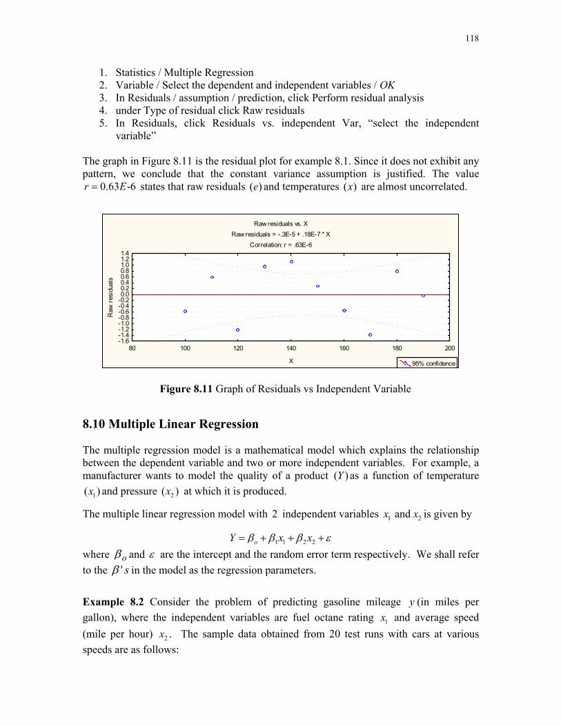
variable” The graph in Figure 8.11 is the residual plot for example 8.1. Since it does not exhibit any pattern, we conclude that the constant variance assumption is justified. The value

0.63 -6r E= states that raw residuals ( )e and temperatures ( )x are almost uncorrelated.

Figure 8.11 Graph of Residuals vs Independent Variable

8.10 Multiple Linear Regression The multiple regression model is a mathematical model which explains the relationship between the dependent variable and two or more independent variables. For example, a manufacturer wants to model the quality of a product ( )Y as a function of temperature

1( )x and pressure 2( )x at which it is produced.

The multiple linear regression model with 2 independent variables 1 2and x x is given by

1 1 2 2oY x xβ β β ε= + + + where oβ and ε are the intercept and the random error term respectively. We shall refer to the s'β in the model as the regression parameters.

Example 8.2 Consider the problem of predicting gasoline mileage y (in miles per gallon), where the independent variables are fuel octane rating 1x and average speed (mile per hour) 2x . The sample data obtained from 20 test runs with cars at various speeds are as follows:

Raw residuals vs. XRaw residuals = -.3E-5 + .18E-7 * X

Correlation: r = .63E-6

80 100 120 140 160 180 200

X

-1.6-1.4-1.2-1.0-0.8-0.6-0.4-0.20.00.20.40.60.81.01.21.4

Raw

resi

dual

s

95% confidence

119

y 1x 2x

24.8 88 52 30.6 93 60 31.1 91 28 28.2 90 52 31.6 90 55 29.9 89 46 31.5 92 58 27.2 87 46 33.3 94 55 32.6 95 62 30.6 88 47 28.1 89 58 25.2 90 63 35.0 93 54 29.2 91 53 31.9 92 52 27.7 89 52 31.7 94 53 34.2 93 54 30.1 91 58

Estimate the linear regression model and interpret your results. Solution To solve this problem by using Statistica, you must be in Multiple Regression module and follow the steps:

1. Enter the values of each variable in a separate column ( or variable) 2. Statistics / Multiple Regression 3. Variables ( select the dependent variable from the list on the left) 4. Hold down the Ctrl key and select the independent variables from the list on the

right. 5. OK 6. In Advanced Click Summary: Regression Results

For the data in Example 8.2, one can read the estimates of the regression parameters as : 1075001931795156 21 .ˆ,.ˆ,.ˆ

o −==−= βββ (See column labeled B in Figure 8.12).

120

Figure 8.12 Regression Summary Thus, the predicted multiple linear regression model for the given data is

1 2ˆ 56.7951 1.0193 0.1075y x x= − + − If 'average speed' ( 2x or Var3) is held fixed, it is estimated that a 1-unit increase in octane ( 1x or Var2) would result in 1.0193 unit increase in the expected 'gasoline mileage'. Similarly if 'octane' ( 1x or Var2) is held fixed, it is estimated that a 1-unit increase in average speed ( 2x or Var3) would result in, 0.1075 unit decrease in the expected 'gasoline mileage'.

121

Exercises 8.1 (cf. Devore, J. L., 2000, 510). The following data represent the burner area

liberation rate ( )x= and emission rate (Nox) ( )y= :

x 100 125 125 150 150 200 200 250 250 300 300 350 400 y 150 140 180 210 190 320 280 400 430 440 390 600 610

(a) Assuming that the simple linear regression model is valid, obtain the least

square estimate of the true regression line. (b) What is the estimate of the expected Nox emission rate when burner area

liberation rate equals 225? (c) Estimate the amount by which you expect Nox emission rate to change when

burner area liberation rate is decreased by 50. 8.2 (cf. Devore, J. L., 2000, 510). The following data represent the wet deposition

(NO3) ( )x= and lichen N (% dry weight) ( )y= :

x 0.05 0.10 0.11 0.12 0.31 0.42 0.58 0.68 0.68 0.73 0.85 y 0.48 0.55 0.48 0.50 0.58 0.52 0.86 1.0 0.86 0.88 1.04

(a) What are the least square estimates of 10 ββ and ? (b) Predict lichen N for an NO3 deposition value of 0 .5. (c) Test the significance of regression at 5% level of significance.

8.3 (Devore, J. L., 2000, 510). The following data represent x = available travel space

in feet, and y = separation distance:

x 12.8 12.9 12.9 13.6 14.5 14.6 15.1 17.5 19.5 20.8 y 5.5 6.2 6.3 7.0 7.8 8.3 7.1 10.0 10.8 11.0

(a) Derive the equation of the estimated line. (b) What separation distance would you predict if available travel space value is

15.0? 8.4 (Devore, J. L., 2000, 511). Consider the following data set in which the variable of

interest are x = commuting distance and y = commuting time:

x 15 16 17 18 19 20 5 10 15 20 25 50 5 10 15 20 25 50y 42 45 35 42 49 46 16 32 44 45 63 115 8 16 22 23 31 60

Obtain the least square estimate of the regression model. 8.5 (cf. Devore, J. L., 2000, 584). Soil and sediment adsorption, the extent to which

chemicals collect in a condensed form on the surface, is an important characteristic influencing the effectiveness of pesticides and various agricultural chemicals, The article “Adsorption of Phosphate, Arsenate, Methancearsonate, and Cacodylate by Lake and Stream sediments: Comparisons with Soils” (J. of

122

Environ. Qual., 1984: 499-504) gives the accompanying data on y = phosphate adsorption index, 1x = amount of extractable iron, and 2x = amount of extractable aluminum.

x1 61 175 111 124 130 173 169 169 160 244 257 333 199x2 13 21 24 23 64 38 33 61 39 71 112 88 54 y 4 18 14 18 26 26 21 30 28 36 65 62 40

(a) Find the least square estimates of the parameters and write the equation of the estimated model.

(b) Make a prediction of Adsorption index resulting from an extractable iron = 250 and extractable aluminum = 55.

(c) Test the null hypothesis that 02 =β against the alternative hypothesis that 02 ≠β at 5% level of significance.

8.6 (Johnson, R. A., 2000, 345). The following table shows how many weeks a sample

of 6 persons have worked at an automobile inspection station and the number of cars each one inspected between noon and 2 P.M. on a given day:

Number of weeks employed (x) 2 7 9 1 5 12 Number of cars inspected (y) 13 21 23 14 15 21

(a) Find the equation of the least squares line, which will enable us to predict y in

terms of x . (b) Use the result of part (a) to estimate how many cars someone who has been

working at the inspection station for 8 weeks can be expected to inspect during the given 2-hour period.

8.7 (cf. Devore, J. L., 2000, 590). An investigation of die casting process resulted in the

accompanying data on 1x = on furnace temperature, 2x = die close time and y = temperature difference on the die surface (A Multiple Objective Decision Making Approach for Assessing Simultaneous Improvement in Die Life and Casting Quality in a Die Casting Process,” Quality Engineering, 1994: 371-383).

x1 1250 1300 1350 1250 1300 1250 1300 1350 1350 x2 6 7 6 7 6 8 8 7 8 y 80 95 101 85 92 87 96 106 108

(a) Write the equation of the estimated model. (b) Test the null hypothesis that 01 =β against the alternative hypothesis that

01 ≠β at 5% level of significance.

8.8 (cf. Johnson, R. A., 2000, 334). The following are measurements of the air velocity

and evaporation coefficient of burning fuel droplets in an impulse engine:

123

Air Velocity (cm/sec) x 20 60 100 140 180 220 160 300 340 380

Evaporation coefficient mm2/sec) y

0.18 0.37 0.35 0.78 0.56 0.75 1.18 1.36 1.17 1.65

(a) Fit a straight line to the data by the method of least square and use it to estimate

the evaporation coefficient of a droplet when the air velocity is 190 cm/s. (b) Test the null hypothesis that 01 =β against the alternative hypothesis 01 ≠β at

the 0.05 level of significance. 8.9 (Johnson, R. A., 2000, 344). A chemical company, wishing to study the effect of

extraction time on the efficiency on an extraction operation, obtained the data shown in the following table;

Extraction time (minutes) (x) 27 45 41 19 35 39 19 49 15 31Extraction efficiency (%) (y) 57 64 80 46 62 72 52 77 57 68

(a) Draw a scattergram to verify that a straight line will provide a good fit to the data.

(b) Draw a straight line to predict the extraction efficiency one can expect when the extraction time is 35 minutes.

8.11 (cf. Johnson, R. A., 2000, 347). The cost of manufacturing a lot of certain product

depends on the lot size, as shown by the following sample data:

Cost (Dollars) 30 70 140 270 530 1010 2500 5020 Lot Size 1 5 10 25 50 100 250 500

(a) Draw a scattergram to verify the assumption that the relationship is linear, letting lot size be x and cost y .

(b) Fit a straight line to these data by the method of least squares, using lot size as the independent variable, and draw its graph on the diagram obtained in part (a).

8.12 (Johnson, R. A., 2000, 345). The following table, x is the tensile force applied to a

steel specimen in thousands of pounds, and y is the resulting elongation thousands of an inch:

x 1 2 3 4 5 6 y 14 33 40 63 76 85

(a) Graph the data to verify that it is reasonable to assume that the regression of Y on x is linear.

(b) Find the equation of the least square line, and use it to predict the elongation when the tensile force is 3.5 thousand pounds.

124 8.13 (Johnson, R. A., 2000, 385). The following are the data on the number of twists

required to break a certain kind of forged alloy bar and the percentage of two alloying elements present in the metal;

No. of twists ( y ) 41 49 69 65 40 50 58 57 31 36 44 57 19 31 33 43 %age Element A ( 1x ) 1 2 3 4 1 2 3 4 1 2 3 4 1 2 3 4 %age Element B ( 2x ) 5 5 5 5 10 10 10 10 15 15 15 15 20 20 20 20

Fit a least square regression plane and use its equation to estimate the number of twists required to break one of the bars when 1x = 2.5 and 2x = 12.

8.14 (Johnson, R. A., 2000, 263). Twelve specimens of cold-reduced sheet steel, having different copper contents and annealing temperatures, are measured for hardness with the following results:

Hardness 78.9 65.1 55.2 56.4 80.9 69.7 57.4 55.4 85.3 71.8 60.7 58.9 Copper content 0.02 0.02 0.02 0.02 0.10 0.10 0.10 0.10 0.18 0.18 0.18 0.18 Annealing Temp. 1000 1100 1200 1300 1000 1100 1200 1300 1000 1100 1200 1300

Fit an equation of the form 2211 xxy o βββ ++= , where 1x represents the copper content, 2x represents the annealing temperature, and y represents the hardness.

8.15 Suppose the following data gives the mass of adults in kilograms sampled from three villages , ,A B C

A B C 71.5 68.0 62.0 65.0 60.5 62.8 63.3 73.5 71.3 73.1 58.4 58.7 73.6 74.1 64.7 72.5 65.5 58.1 78.1 73.6 66.0 73.0 50.6 58.5 66.5 76.5 72.6 66.8 62.1 52.6 74.3 73.3 71.1 71.9 64.5 58.8 76.3 76.0 65.4 65.0 60.6 63.7 62.0 64.0 59.1 69.9 62.9 61.6 62.8 69.6 69.7 69.8 60.2 67.2 72.9 69.2 77.1 78.5 63.4 58.2

(a) Assuming that these samples are independent, run t-tests to determine which of the villages have identical mean mass of adults stating clearly the hypotheses you are testing. State your conclusions based on the -valuep as well as the t-value.

(b) State the assumption under which your tests are valid.

8.16 (cf. Dougherty, 1990, 595) When smoothing a surface with an abrasive, the roughness of the finished surface decreases as the abrasive grain becomes finer. The following data give measurements of surface roughness (in micrometers) in terms of the grit numbers of the grains, finer grains possessing larger grit numbers.

x 24 30 36 46 54 60 y 0.34 0.30 0.28 0.22 0.19 0.18

(a) Draw a scatter diagram. Do you recommend fitting a linear regression model?

125

(b) How strong is the linear correlation between the two variables? (c) Do you think that there is strong nonlinear correlation between the two variables?

8.17 (cf. Johnson, R. A., 2000, 578). The article “ How to optimize and Control the Wire Bonding Process: Part II” (Solid State Technology, Jan. 1991: 67-72) described on experiment carried out to assess the impact of the variable 1x = force (gm), 2x = power (mw), 3x = temperature ( C ), and 4x = time (ms) on y = ball bond share strength (gm). The following data generated to be consistent with the information given in the article:

Observations Force Power Temperature Time Strength 1 30 60 175 15 26.22 40 60 175 15 26.3 3 30 90 175 15 39.8 4 40 90 175 15 39.7 5 30 60 225 15 38.6 6 40 60 225 15 35.5 7 30 90 225 15 48.8 8 40 90 225 15 37.8 9 30 60 175 25 26.6 10 40 60 175 25 23.4 11 30 90 175 25 38.6 12 40 90 175 25 52.1 13 30 60 225 25 39.5 14 40 60 225 25 32.3 15 30 90 225 25 43.0 16 40 90 225 25 56.0 17 25 75 200 20 35.2 18 45 75 200 20 46.9 19 35 45 200 20 22.7 20 35 105 200 20 58.7 21 35 75 150 20 34.5 22 35 75 250 20 44.0 23 35 75 200 10 35.7 24 35 75 200 30 41.8 25 35 75 200 20 36.5 26 35 75 200 20 37.6 27 35 75 200 20 40.3 28 35 75 200 20 46.0 29 35 75 200 20 27.8 30 35 75 200 20 40.3

(a) Find the least square estimates of the parameters and write the equation of the

estimated model. (b) Make a prediction of strength resulting from a force of 35 gm, power of 75 mw,

temperature of 200 degrees and time of 20 ms. (c) Test the null hypothesis that 03 =β against the alternative hypothesis that

03 ≠β at 5% level of significance.