chapter 8—application and interpretation of …

8-1

CHAPTER 8—APPLICATION AND INTERPRETATION OF CONGESTION MEASURES

Chapter Summary

The focus of this chapter is to provide the reader with practical applications and

interpretation of the congestion measures described in this report. This chapter discusses the application of techniques at different levels of analysis, including multimodal as well as long and short roadway sections. The sample applications include both an arterial and freeway roadway along the same corridor. The spreadsheet that includes the computations performed in this chapter is available at http://mobility.tamu.edu/resources. The spreadsheet can be downloaded and altered for specific analyses of interest.

While the spreadsheet applications primarily provide examples of congestion analyses that might be obtained from travel demand models or travel time runs, there is an example provided at the end of this chapter that illustrates typical mobility analysis using real-time (ITS) data. The final workbook of the spreadsheet includes the computation of mobility measures from an ITS data source.

This chapter will provide numerous applications of the performance measures defined

and discussed in this paper. The examples include multimodal, corridor, and traffic operations improvement analyses. Many of the examples are updated from their initial presentation in Quantifying Congestion (1). 8.1 Application of Techniques at Different Levels of Analysis

Developing a system of congestion measures should be initiated only after an

examination of the uses, users, and audiences to be served, and after full considerations of program goals and objectives and the nature of likely solutions. This chapter illustrates a system of travel time-based measures to estimate congestion levels. Chapter 5 introduced most of these mobility measurements. The procedures in this chapter are useful for roadway systems, other person and freight movement modes, and transportation improvement strategies and programs. Although a number of analyses may not benefit from such a broad focus, consideration of the context in which the measures are to be used will allow the user to identify the appropriate set of congestion measures.

Congestion measures are applied in different geographic settings, in different time

frames, at differing levels of detail, at different scales, and under existing, changed, and future conditions. They must accurately describe present conditions and be capable of being forecast. There is a need for measures that can be applied across all passenger modes of urban travel individually and simultaneously. The majority of congestion measure applications remain highway oriented, but with increased emphasis on the movement of people.

http://mobility.tamu.edu/resources

8-2

The following sections describe techniques for measuring congestion on various sections of a transportation network. Examples are used to illustrate the application of the basic measures to typical situations of system evaluation or analysis of alternative improvements. Single mode and multimodal systems are integrated in the examples. 8.1.1 Applying Analysis Methods

The research clearly indicates the need to separate the issues of data collection from the

measures that are used in technical analyses and presentations. The measures that are needed to evaluate the transportation system or the effect of improvements are the most important consideration. Data collection or measurement estimates can be developed in a variety of ways; these are important elements of a congestion monitoring program, but they should not be the key consideration in deciding which measures are used.

While direct measurement of travel time and speed is desirable for evaluation of existing

congestion, it is not always practical. Moreover, when future conditions are analyzed, the travel time data that would be helpful in assessing potential effects of operational improvements or judging the cost-effectiveness of additional roadway lanes are obviously not available to be collected. Travel time and speed estimating procedures are needed for situations like this and are thus an important part of the congestion measurement process. Overall, there are several ways to accomplish measurement and estimation of congestion information.

The travel time and speed estimating procedures that are needed include relatively simple

procedures that use easily obtained data, procedures that can be used by agencies responsible for system operations, and procedures that work well with travel demand models.

Exhibit 8-1 shows how the three basic categories of analysis relate to the four most

common types of analysis. It serves as a general guide for practitioners to generate congestion information and to identify the appropriate data collection and analysis strategies.

• Purpose—For most types of general policy, programming, or planning purposes, the

surrogate estimation procedures will provide useful results with a minimum of data collection. More specific design and operation concerns will require more precision, and direct measures of travel time or travel speed will usually be required.

• Analysis period—Most techniques can produce useful information for existing

conditions, but future conditions will require some surrogate procedures (e.g., travel time or HCM). Surrogates will also be required for existing conditions where future scenarios will be analyzed. This approach will provide uniformity of estimation, avoiding inconsistencies associated with differences in roadway system operations.

• Analysis scope and scale—HCM analysis procedures will be used for most

intersection analyses and possibly for short roadway segments; direct travel time measures will be more useful for analysis areas greater than short roadway segments. If large corridors, sub-areas, or regions are to be analyzed, some sampling process will be useful to limit data collection requirements.

8-3

Exhibit 8-1. Applications of Congestion Analysis Methods.

Analysis Category

Type of Analysis Method Highway Capacity Manual

Direct Travel Time

Measurement

Sampling Travel Time on Segments

Surrogate Travel Time Procedures

Purpose Policy Analysis L Project Prioritization L Planning or Alternative Analysis L L Design L L Operation L

Analysis Period Existing Conditions L L L •1 Future Conditions

Short range L L L •1 Long range L

Analysis Scope and Scale Intersections L Single Roadway L Corridor L L Sub-area L L Areawide L L

Source: NCHRP (1) Application in most analyses Τ Limited application 1 Particularly when needed as base condition for analysis of future conditions 8.1.2 Free-flow Travel Conditions

If estimated free-flow travel rates or speeds are used in the calculation of delay, the speed data collected from field studies may include values with faster speeds or lower rates. Computerized analysis procedures should be modified so that a “negative delay” value is not included in the calculations (as done in the examples in this chapter). 8.1.3 Travel Rate Index and Travel Time Index

It is important to recognize the fundamental differences between the Travel Rate Index and the Travel Time Index. Chapter 5 described the TTI in detail and provided an equation for computation. It should be noted that the TTI includes the impacts of incident conditions on congestion for the analysis period. Incident effects can be difficult to account for unless they are inherently included in the data source. Archived ITS (real-time) data include the effects of incidents because they monitor continuously. Therefore, the data captures the effects of recurring and incident conditions in the speed, volume, and occupancy information that they collect. Post-processing of travel demand model data can also be performed to estimate the effects of incidents to obtain TTI values. This can be done by estimating incident factors. Incident delay factors (the ratio of incident to recurring delay) are used in the Urban Mobility Report to include the effects of incidents.

8-4

Typically, incident conditions are not included for corridor studies along which travel time runs are performed. Incident-free conditions are often desired with travel time runs that have a limited number of travel time runs. To ensure the limited sample of travel time data collection are not “skewed” by falsely including a run or two that might include an incident condition, incident runs are usually removed from the travel time data set. Assuming an adequate sample, and by removing runs that include incidents, the resulting travel time data set provides an estimate of the recurring congestion along the corridor. In these conditions, the computed measure would be a TRI because it is computed with travel rates that do not include incident conditions (i.e., recurring congestion only). TRI is computed mathematically the same way as the TTI, but it does not include incident conditions.

Exhibit 8-2 graphically illustrates the difference between the TRI (includes recurring congestion only) and the TTI (includes both recurring and incident congestion). The spreadsheet applications in this chapter include a user-input percent of incident delay from which the performance measures are computed that include incidents.

Exhibit 8-2. Relationship between TTI and TRI over Time.

8.1.4 Common Data for All Examples

The basic formulas for congestion measurement are listed in Exhibit 8-3. More information on the measures can be found in Chapter 5. This summary is provided for easy reference in the examples. More specifically, Exhibit 8-4 describes the calculations and format used in the examples. The lines of data are labeled, and the calculations refer to the labels so that the information is easy to understand and code into spreadsheet or database formats. The first column of Exhibit 8-4 shows a discontinuity in the alphabetical data labels because the delay values and congested travel summary are shown in comparison to the “free-flow travel rate” conditions for illustration. The spreadsheet used for the calculations of the examples in this chapter is available at http://mobility.tamu.edu/ums, and it contains calculations relative to target, free-flow, and posted speed limit travel rates.

1.00

1.05

1.10

1.15

1.20

1.25

1.30

1.35

1.40

1982

1983

1984

1985

1986

1987

1988

1989

1990

1991

1992

1993

1994

1995

1996

1997

1998

1999

2000

2001

2002

2003

Year

Inde

x Va

lue Travel Time Index

(TTI)

Travel Rate Index(TRI)

Incident CongestionComponent

Recurring CongestionComponent

Total CongestionEffect

http://mobility.tamu.edu/ums

8-5

Exhibit 8-3. Quick Reference Guide to Selected Mobility Measures. INDIVIDUAL MEASURES1

Delay per Traveler

( )( ) ( ) ( ) ( )

( ) ( )hiclepersons/veOccupancy Vehicle vehicles

Volume Vehicle

minutes 60hour

year weekdays250 hiclepersons/ve

Occupancy Vehicle vehiclesVolume Vehicle

minutesTime TravelPSL or FFS

- minutes

Time TravelActual

hours annual

TravelerperDelay

×

××××

=

Travel Time ( ) ( ) ( ) ( ) ( )hiclespersons/veOccupancy Vehicle vehicles

Volume Vehicle milesLength mileperinutesm

RateTravelActual minutespersonTimeTravel ×××=−

Travel Time Index2

( )

( )mileperminutesRateTravel PSL or FSF

mileperminutesRateTravelActual

IndexTimeTravel =

Buffer Index2 ( ) ( ) ( )

( )100%

minutesTime Travel Average


minutesTime Travel Percentile 95th

% Index Buffer ×

−=

Planning Time Index2 ( )

( )

( )minutesTime Travel PSL or FSF

minutesTime Travel Percentile 95

units noIndex Time Planning

th

=

AREA MOBILITY MEASURES1

Total Delay ( ) ( ) ( ) ( ) ( )hiclepersons/veOccupancy Vehicle

vehiclesVolume Vehicle

minutesTime TravelPSL or FFS

- minutes

Time TravelActual

= minutes-personDelay SegmentTotal ××

Congested Travel ( ) ( ) ( )

×∑ vehicles

Volume Vehicle miles

Length SegmentCongested

= miles-vehicleTravel Congested

Percent of Congested

Travel

( ) ( ) ( ) ( )

( ) ( ) ( ) ( )

100

hiclepersons/veOccupancy

icleehV

vehiclesVolumeVehicle

milesLength mile per minutes

Rate Travel Actual

hiclepersons/veOccupancy

icleehV

vehiclesVolumeVehicle

minutesTimeTravel

PSL or FFS

-

minutesTimeTravelActual

TravelCongested

ofPercent

n

i segmentsAll

iiii

segmentcongested Each

m

1iii

ii

×

×××

××

=

∑

∑

=

=

1

Congested Roadway ( ) ( )miles Lengths

SegmentCongested = milesRoadway Congested ∑

Accessibility ( ) ( )Time Travel Target Time Travel

Where ,jobs e.g., ortunitiesOpp tFulfillmen Objective

= iesopportunitityAccessibil

≤

∑

1“Individual” measures are those measures that relate best to the individual traveler, whereas the “area” mobility measures are more applicable beyond the individual (e.g., corridor, area, or region). Some individual measures are useful at the area level when weighted by PMT (Passenger Miles Traveled) or VMT (Vehicles Miles Traveled).

2Can be computed as a weighted average of all sections using VMT or PMT). Note: FFS = Free-flow speed, PSL = Posted speed limit.

8-6

Exhibit 8-4. Formula Descriptions for Congestion Measurement Examples. Label Measure Units Description

a Length Miles input value b Vehicle Volume Vehicles collected value c Average Vehicle Occupancy Persons/Vehicle collected value d Percent Incident Delay Percent collected value Speeds e Free-flow Speed Miles/Hour collected value f Speed limit Miles/Hour collected value g Target Speed Miles/Hour collected value h Non-incident Speed Miles/Hour collected value i Estimated Actual Speed Miles/Hour (g x a x b x c) / ( [g x bp] ) + [a x b x c] )

Initial Computations j Person Volume Persons b x c k Vehicle-miles Vehicle-miles a x b l Person-miles Person-miles j x a Travel Rates

m Free-flow Travel Rate Minutes/Mile 60 / e n Speed Limit Travel Rate Minutes/Mile 60 / f o Target Travel Rate Minutes/Mile 60 / g p Non-incident Travel Rate Minutes/Mile 60 / h q Estimated Actual Travel Rate Minutes/Mile 60 / i Travel Times r Free-flow Travel Time Person-Hours (l x m) / 60 s Speed Limit Travel Time Person-Hours (l x n) / 60 t Target Travel Time Person-Hours (l x o) / 60 u Non-incident Travel Time Person-Hours (l x p) / 60 v Estimated Actual Travel Time Person-Hours (l x q) / 60 Total Delay Rate

w vs. free-flow Minutes/Mile q - m x vs. speed limit Minutes/Mile q - n y vs. target Minutes/Mile q - o z Std. Dev. of Actual Travel Rate Minutes/Mile collected value

Recurring Delay Computations (Supports Mobility Measures) Recurring Delay Rate

aa vs. free-flow Minutes/Mile p - m Recurring Delay (vs. free-flow)

ad Vehicle Travel Vehicle-Hours (k x aa) / 60 ae Person Travel Person-Hours (l x aa) / 60

Mobility Performance Measures Computations Congested Travel Summary

ay Person-Miles (vs. free-flow) Person-Hours Sum of congested person-miles (line l if line w is greater than zero)

bb Person-Hours (vs. free-flow) Person-Hours Sum of congested person hours (line v if line w is greater than zero)

be Miles of Congested Roadway (vs. free-flow)

Miles Sum of congested miles (line a if line w is greater than zero)

Percent of Congested Travel

bh vs. free-flow Percent (bb / v) x 100 Total Delay (vs. free-flow)

bk Vehicle Travel Vehicle-Hours ad / (1 - d/100) bl Person Travel Person-Hours ae / (1 - d/100) Total Delay (vs. free-flow) per:

bw Person-Mile Person-Minutes (bl x 60) / l bx Mile of Road Person-Hours bl / a Travel Time Index

cc vs. free-flow Travel Rate Ratio q / m Note: See Section 5.4 for further explanation of speed terms and application guidance.

8-7

Exhibit 8-5 presents the free-flow speeds used in the examples. Exhibit 8-6 shows the target TTI values used in the examples. In a typical application, the target TTI values would be developed with input from citizens, businesses, decision makers, and transportation professionals. They represent the crucial link between 1) the vision that the community has for its transportation system, land uses, and its “quality of life” issues and 2) the improvement strategies, programs, and projects that government agencies and private sector interests will implement. The values are desirably the result of a process that is integrated with the development of the long-range plan, but they must be reasonable and realistic, since overstatement or understatement could distort congestion assessment. The level of information needed to carry out this type of process at an optimum level is not currently distributed in most urban areas. The values can, however, be interpreted from existing input processes. The values in Exhibit 8-5, Exhibit 8-6, and Exhibit 8-7 are for illustration purposes only.

Exhibit 8-5. Free-flow Speed (mph) Used in the Examples.

Freeway Mainlane Freeway HOV Major Street Bus on Street Rail in Street Bike

60 60 35 15 20 15

Exhibit 8-6. Target TTI Used in the Examples. Area Type Peak Off-peak

Central Business District 1.7 1.2 Central City/Major Activity Center 1.5 1.1 Suburban 1.3 1.0 Fringe 1.0 1.0

Exhibit 8-7. Target Peak and Off-peak Speeds (mph).

Area Type

Freeway Mainlane

Freeway HOV Major Street Bus on Street Rail in Street Bike

Peak Off-peak Peak

Off-peak Peak

Off-peak Peak

Off-peak Peak

Off-peak Peak

Off-peak

Central Business District 35 50 35 50 21 29 9 13 12 17 9 13

Central City /Major Activity Center 40 55 40 55 23 32 10 14 13 18 10 14

Suburban 46 60 46 60 27 35 12 15 15 20 12 15 Fringe 60 60 60 60 35 35 15 15 20 20 15 15

The examples in this section are for several levels of analysis from isolated locations to

regional analyses, but they are based on individual facility evaluations. These include segments of freeways and streets, with general-purpose traffic, as well as buses, rail transit, and carpools. The examples also show several alternative improvements that might be proposed to address congestion and mobility problems including better operational efficiency, increases in transit and rideshare use, and improvements in operations through improved traffic signals and incident response.

Urban areas should approach the use of target travel rates with a systemwide strategy.

They should recognize that the targets may not be achievable for every roadway situation. Other travel mode improvements, strategies, or policies may be needed. For example, the target speeds shown in Exhibit 8-7 do not equate to slow enough speeds to justify an HOV lane under normal

8-8

circumstances. It is likely, however, that the freeway speeds will be lower than those in Exhibit 8-7 in most large urban areas. An HOV lane can contribute to bringing the Travel Time Index for the corridor, when weighted by person volume, closer to the target value.

The examples are focused on the appropriate level of detail necessary to identify the effect of a proposed treatment. For most alternatives, this is at the corridor level or more detailed; this is the area where the effect of the improvement can be identified and the reasonableness of the measurement techniques can be checked. The magnitude of the numbers for a wider area may mask the impact of a single improvement, especially for relatively small changes. The corridor level of analysis is also where most projects are evaluated, prioritized, and funded.

Focusing on individual facilities or modes, however, is not consistent with the manner in which most travelers make their choices. Door-to-door travel time is closer to the primary measure used by travelers and is best expressed in accessibility measures (see Exhibit 8-3 for more information on the accessibility measure). Unfortunately, it is difficult to translate an accessibility measure like “population within 30 minutes’ travel time of a major activity center” into a procedure to evaluate signal improvements on an arterial street. The transportation and land use planning model required to calculate the accessibility may not be sensitive enough to identify the improvement in travel conditions.

The method to connect accessibility measures with the many smaller scale analyses is the

target travel condition values. The target Travel Time Index and associated speeds identify when citizens believe improvements should be made. The conditions that citizens find unacceptable will be a mix of economic development, transportation, and quality of life considerations. The discussion about what constitutes unacceptable conditions could be conducted in conjunction with the long-range planning process and the future visions of the area.

The examples depict peak-hour conditions, but the same procedures could be used for

peak-period, off-peak periods, or daily analyses. The weighting process used in the examples to calculate averages and totals for different modes and sections of roadway—using person-volume—is the same one used to calculate peak period and daily measures. The peak hour focus used here allows the users to see the calculation procedures and usage of the statistics. Post-project evaluations may show no improvement in peak hour performance, but there may be reductions in the length of the peak period that are affected by congestion. 8.1.5 Individual Locations

Analyses of intersections should be performed according to the 2000 Highway Capacity Manual procedures or other commonly accepted intersection or site analysis procedures. Stopped delay intersection studies can be used to directly collect delay information. Observations of traffic backups—their extent and duration—are very useful.

It is difficult to apply travel time and speed study types to the analysis of intersections.

Floating car runs or license plate matching studies are not very meaningful for short distances in which one signal controls the variability of travel speeds. As traffic signals are connected into

8-9

systems, however, it will become more difficult to analyze any intersection in isolation, and longer sections of roadway will become the basic unit for more analyses.

Traditional measures of service quality at signalized intersections include stopped delay per vehicle and the number of stops. It is suggested that the measures of delay and delay per vehicle or per person be considered for intersection congestion studies. These measures are consistent with current intersection analysis measures and provide the ability to calculate quantities that reflect the importance of person movement. These quantities can be developed from direct data collection efforts or from the Highway Capacity Manual procedures. Accessibility can be used to estimate the effect of transportation conditions on travel associated with localized site development but has little applicability to evaluating traffic operations at individual locations.

Short Roadway Sections

The analysis of short roadway sections, on the magnitude of 1 to 4 miles, differs

somewhat from the analysis of longer roadway sections. Short roadway sections may match existing divisions of roadway inventory data or could include several relatively homogenous roadway links between intersections and interchanges. These individual roadway links within a short section should have similar cross sections, traffic volumes, and operating conditions. Individual links that have different cross sections or operating conditions should not be combined together to form a short roadway section. Instead, roadway links with different characteristics should be considered separately or with other adjacent links that have similar characteristics.

The use of travel time and travel rate data is well suited to the analysis of roadway

sections. Travel times between intersections or interchanges can be added to match the appropriate section length. Because the cross section and traffic volumes are similar for each link, a single average or representative data value can be used to represent all links within a section. Congestion on short sections can be identified by comparing the actual Travel Time Index to the target Travel Time Index.

Suggested Measures. Appropriate measures for short roadway sections include the

average travel rate, delay rate, total segment delay, and the Travel Time Index. These measures will provide useful information at this level of analysis. The average travel rate, delay rate, and Travel Time Index can be used in absolute terms or can be used to compare similar classes of facilities. The total delay and Travel Time Index can be used to compare different classes of facilities.

Highway Capacity Manual procedures may be used to develop estimates for these

quantities. However, in severely congested corridors or for before/after studies of coordinated or adaptive signal systems (systems that can change timing plans several times during the peak in response to demand), direct data collection studies will be more appropriate and useful in estimating congestion levels.

8-10

Example. Exhibits 8-8 and 8-9 illustrate several key congestion statistics for a freeway and a major street. These statistics are similar to those that would be used if a congestion evaluation were performed on an individual facility or as one part of an areawide analysis. License plate matching, floating car travel time runs, or automated vehicle monitoring could be used to develop the travel time and speed information. Roadway inventory files could be used to identify logical section limits as well as other useful information, such as the number of lanes.

Main Street. Two sections of four-lane Main Street are displayed in Exhibit 8-8. The

auto and bus modes are separated because the travel speed and vehicle occupancy rates are significantly different. Improvements to the sections may also change the travel characteristics of the modes differently, so the data were collected separately. The total or average column presents information on both sections together.

The length, volume, and person-miles of travel are used in calculating cumulative

statistics and in weighting for average statistics. The target speeds are less than the free-flow speeds, indicating that some level of congestion is considered acceptable for this portion of the system. The actual travel rates are higher than the target rates, indicating a need for improvements to attain the target travel rates.

The most useful statistics for evaluations are found in lines v through bs. Note that

additional calculations are included in the attached spreadsheet. This is why the alphabetical label names are discontinuous. The delay rate is calculated relative to the free-flow speed, target speed, and speed limit. The target travel rate is the value that would be used to compare alternative improvement projects, while the free-flow comparison is useful in quantifying areawide congestion levels. The delay values are the cumulative statistics that would be used in estimating the benefit/cost relationship for new projects or improvement strategies.

The TTI for this suburban corridor is 1.55 when comparing to the target speed. In

comparison with Exhibit 8-6, this indicates that improvements are necessary to meet the target TTI value of 1.3.

Southside Freeway. The statistics for this section of six-lane Southside Freeway are the

same type as those presented for Main Street. This section of Southside Freeway is also congested relative to both free-flow and target values. The bus volume on the freeway is double that on Main Street, but the autos in the freeway mainlanes carry many more persons than the buses such that the cumulative statistics are governed by the auto travel conditions. Since the buses are not stopping on the freeway, as they do on the street, their performance statistics are very similar to the autos with respect to speed and speed reliability.

8-11

Exhibit 8-8. Existing Operation on Main Street Example. Roadway Name: Main Street

Location: 71st to 89th Street (Suburban) Travel Period: Morning Peak Hour

Travel Direction: Northbound (Peak Direction) Alternative: Existing Operation

Label Measure Units

System Element

Total or Average

71st Street to 80th Street

80th Street to 89th Street

Auto Bus Auto Bus a Length Miles 2.8 2.8 3.5 3.5 6.3 b Vehicle Volume Vehicles 1000 8 1200 10 c Average Vehicle Occupancy Persons/Vehicle 1.20 31.25 1.21 30.00 1.44 d Percent Incident Delay Percent 40 40 50 50 Speeds e Free-flow Speed Miles/Hour 35 15 35 15 28 f Speed limit Miles/Hour 30 30 30 30 30 g Target Speed Miles/Hour 25 15 25 15 22 h Non-incident Speed Miles/Hour 20 12 15 10 15 i Estimated Actual Speed Miles/Hour 18 11 11 8 12

Initial Computations j Person Volume Persons 1,200 250 1,452 300 k Vehicle-miles Vehicle-miles 2,800 22 4,200 35 7,057 l Person-miles Person-miles 3,360 700 5,082 1,050 10,192 Travel Rates

m Free-flow Travel Rate Minutes/Mile 1.71 4.00 1.71 4.00 2.11 n Speed Limit Travel Rate Minutes/Mile 2.00 2.00 2.00 2.00 2.00 o Target Travel Rate Minutes/Mile 2.40 4.00 2.40 4.00 2.67 p Non-incident Travel Rate Minutes/Mile 3.00 5.00 4.00 6.00 3.95 q Estimated Actual Travel Rate Minutes/Mile 3.40 5.67 5.60 8.00 5.13

Travel Times v Estimated Actual Travel Time Person-Hours 190 66 474 140 871

Total Delay Rate

w vs. free-flow Minutes/Mile 1.69 1.67 3.89 4.00 3.02 x vs. speed limit Minutes/Mile 1.40 3.67 3.60 6.00 3.13 y vs. target Minutes/Mile 1.00 1.67 3.20 4.00 2.45 z Std. Dev. of Actual Travel Rate Minutes/Mile 0.5 0.7 0.5 0.7 0.5


aa vs. free-flow Minutes/Mile 1.29 1.00 2.29 2.00

Recurring Delay (vs. free-flow) ad Vehicle Travel Vehicle-Hours 60.0 0.4 160.0 1.2 ae Person Travel Person-Hours 72.0 11.7 193.6 35.0

Mobility Performance Measures Computations Total Delay (vs. free-flow)

bk Vehicle Travel Vehicle-Hours 100 1 320 2 423 bl Person Travel Person-Hours 120 19 387 70 597

Total Delay (vs. free-flow) per:

bw Person-Mile Person-Minutes 2 2 5 4 4 bx Mile of Road Person-Hours 43 7 111 20 72

Travel Time Index

cc vs. free-flow Travel Rate Ratio 1.98 1.42 2.33 1.50 2.07 Note: See Section 5.4 for further explanation of speed terms and application guidance.

8-12

Exhibit 8-9. Existing Operation of Southside Freeway. Roadway Name: Southside Freeway

Location: 71st to 130th Street (Suburban ) Travel Period: Morning Peak Hour


Label Measure Units

System Element

Total or Average

71st Street to 101st Street


Auto Bus Auto Bus a Length Miles 4.4 4.4 4.0 4.0 8.4 b Vehicle Volume Vehicles 5,800 20 5,500 20 c Average Vehicle Occupancy Persons/Vehicle 1.20 32.50 1.20 32.50 1.31 d Percent Incident Delay Percent 50 50 50 50 50 Speeds e Free-flow Speed Miles/Hour 65 65 65 65 65 f Speed limit Miles/Hour 60 60 60 60 60 g Target Speed Miles/Hour 45 45 45 45 45 h Non-incident Speed Miles/Hour 30 30 25 25 27 i Estimated Actual Speed Miles/Hour 23 23 17 17 20

Initial Computations j Person Volume Persons 6,960 650 6,600 650 k Vehicle-miles Vehicle-miles 25,520 88 22,000 80 47,688 l Person-miles Person-miles 30,624 2,860 26,400 2,600 62,484 Travel Rates


Travel Times v Estimated Actual Travel Time Person-Hours 1361 127 1525 150 3,164

Total Delay Rate



aa vs. free-flow Minutes/Mile 1.08 1.08 1.48 1.48

Recurring Delay (vs. free-flow) ad Vehicle Travel Vehicle-Hours 458 2 542 2 ae Person Travel Person-Hours 550 51 650 64

Mobility Performance Measures Computations Total Delay (vs. free-flow)

bk Vehicle Travel Vehicle-Hours 916 3 1,083 4 2,006 bl Person Travel Person-Hours 1,099 103 1,300 128 2,630

Total Delay (vs. free-flow) per:

bw Person-Mile Person-Minutes 2 2 3 3 3 bx Mile of Road Person-Hours 250 23 325 32 262

Travel Time Index`

cc vs. free-flow Travel Rate Ratio 2.89 2.89 2.60 2.60 2.75 Note: See Section 5.4 for further explanation of speed terms and application guidance.

8-13

Long Roadway Sections or Routes

The analysis of long roadway sections or routes, generally greater than 4 to 5 miles, must take into consideration the different operating characteristics of the roadway along the entire length. Routes will contain two or more short roadway sections with different cross sections and operating characteristics. Consequently, congestion studies must recognize and account for the different operating conditions along the route. Average or representative travel time values should be developed for each short roadway section within a route, and various cumulative statistics can be calculated for the entire route.

Suggested Measures. Average statistics, like the average travel rate and the average

delay rate, are weighted by the length of each segment and may be less meaningful for long routes or routes with widely varying conditions. The Travel Time Index is also a good measure. Cumulative statistics, like total delay, congested travel, and congested roadway may provide more useful information for these longer routes. Again, vehicle occupancies should be used to obtain person delay.

Main Street Example. Longer route section summaries can either identify each mode

individually (as in Exhibit 8-8) or present the statistics as a combination of all modes on the route. Exhibit 8-10 shows the simpler nature of the combined mode format for sections with several road segments. The 71st to 89th Street segment statistics are drawn from Exhibit 8-8 and combined with the new 89th to 95th Street segment. The estimated actual travel rate is equal to the target travel rate for 89th to 95th. This is presented as no delay in line af and line am. The standard deviation is also slightly less in the less-congested section, possibly due to the lower volume, which allows for minor incidents to be handled without much impact on traffic flow.

Travel conditions in longer sections are more easily described by the cumulative statistics

in lines ay through bh. Using person-miles of travel to weight the individual section values results in a measure of the average condition seen by the travelers in the 71st to 95th section of Main Street. An average of 3 minutes of delay is incurred by the travelers on Main Street, and an average of 92 person-hours of delay is incurred daily on each mile of this section of Main Street. The Travel Time Index for the entire arterial section is 2.25 (relative to the free-flow travel rate). These averages obviously hide some of the problems between 71st and 89th, but these are identified in the person-miles, person-hours, and miles of congested roadway statistics. These are developed by summing the statistics (for lines a, l, and v) in every section of road that is congested (71st to 95th).

8-14

Exhibit 8-10. Long Section Analysis along Main Street. Roadway Name: Main Street

Location: 71st to 95th Street (Suburban ) Travel Period: Morning Peak Hour


Label Measure Units

System Element Total or Average

71st to 80th (Exhibit 8-8)

80th to 89th (Exhibit 8-8)

89th to 95th (New Section)

a Length Miles 2.8 3.5 2.1 8.4 b Vehicle Volume Vehicles 1,008 1,210 700 c Average Vehicle Occupancy Persons/Vehicle 1.44 1.44 1.44 1.44 d Percent Incident Delay Percent 45 45 50 Speeds e Free-flow Speed Miles/Hour 25 25 25 25 f Speed limit Miles/Hour 30 30 30 30 g Target Speed Miles/Hour 20 20 20 20 h Non-incident Speed Miles/Hour 15 12 25 14 i Estimated Actual Speed Miles/Hour 12 9 20 11

Initial Computations j Person Volume Persons 1,452 1,742 1,008 k Vehicle-miles Vehicle-miles 2,822 4,235 1,470 8,527 l Person-miles Person-miles 4,064 6,098 2,117 12,279 Travel Rates

m Free-flow Travel Rate Minutes/Mile 2.40 2.40 2.40 2.40 n Speed Limit Travel Rate Minutes/Mile 2.00 2.00 2.00 2.00 o Target Travel Rate Minutes/Mile 3.00 3.00 3.00 3.00 p Non-incident Travel Rate Minutes/Mile 4.00 5.00 2.40 4.22 q Estimated Actual Travel Rate Minutes/Mile 4.82 6.64 3.00 5.41

Travel Times v Estimated Actual Travel Time Person-Hours 326 675 106 1,107 Total Delay Rate

w vs. free-flow Minutes/Mile 1.60 2.60 0.00 1.82 x vs. speed limit Minutes/Mile 2.00 3.00 0.40 2.22 y vs. target Minutes/Mile 1.00 2.00 0.00 1.32 z Std. Dev. of Actual Travel Rate Minutes/Mile 0.5 0.5 0.5 0.5


aa vs. free-flow Minutes/Mile 1.60 2.60 0.00 Recurring Delay (vs. free-flow)

ad Vehicle Travel Vehicle-Hours 75 184 0.0 ae Person Travel Person-Hours 108 264 0.0


ay Person-Miles (vs. free-flow) Person-Hours 4,064 6,098 0 10,163 bb Person-Hours (vs. free-flow) Person-Hours 326 675 0 1,001 be Miles of Congested Roadway

(vs. free-flow) Miles 2.8 3.5 0.0 6.3


bh vs. free-flow Percent 100 100 0 83 Total Delay (vs. free-flow)

bk Vehicle Travel Vehicle-Hours 137 334 0.0 471 bl Person Travel Person-Hours 197 481 0.0 678

Total Delay (vs. free-flow) per: bw Person-Mile Person-Minutes 3 5 0.0 3 bx Mile of Road Person-Hours 70 137 0.0 92

Travel Time Index cc vs. free-flow Travel Rate Ratio 2.01 2.77 1.25 2.25

Note: See Section 5.4 for further explanation of speed terms and application guidance.

8-15

Corridors The analysis of congestion along corridors would be similar to a route analysis but could

include parallel freeway and arterial street routes that serve dense travel corridors. At this level of analysis, surrogate measurement techniques could be combined with direct data collection to obtain the necessary information. A calibration process would be required to correlate the direct and surrogate statistics so that variations in estimated travel speed are due to traffic conditions and not due to differences in the measurement technique.

The number of data collection sites could be governed by a statistical sample of the

routes or could be performed for all major movements in the corridor. The calculation of average travel and delay rates for the corridor as a whole would be based on individual segment data. Statistics for each segment could be summed or averaged in discrete quantities (short sections) to form a corridor analysis. The relative delay rate can serve as a method to examine congestion levels on the combination of freeways and streets.

Suggested Measures. Average statistics for travel rate and delay rate are useful for

intermediate calculations, but they may not provide an accurately detailed description of operating conditions and are difficult to interpret or relate to some audiences. Cumulative statistics like total delay, congested travel, and travel time are more meaningful at this level of analysis. The delay rate and Travel Time Index can be used to compare congestion levels on freeways and arterial streets.

Corridor Example. The Main Street and Southside Freeway summary statistics are

presented in Exhibit 8-11 to quantify the corridor congestion level. Total delay, Travel Time Index, and congested travel measures are evaluative statistics that are particularly useful in improvement analyses. They identify the magnitude of the problem and point to some solutions that might be studied. The delay per person quantifies a measure of the intensity of congestion, which is more explainable to the public and is close to the way the public perceives congestion levels. The person delay per mile of road is also a useful value for comparing congestion levels on sections of road with varying lengths and varying transit ridership and rideshare activity.

More relevant values in comparisons between streets and freeways in a corridor are the

delay rate and the Travel Time Index. Relative comparisons are very important to identifying corridors and facilities within those corridors for improvement studies. The process of combining the modes for a corridor average should not overlook the important modal analyses that must also take place to evaluate individual facilities because that is the level where many improvements are made (e.g., more lanes, parking spaces, buses, improved traffic signal systems, improved rideshare programs, and access management policies).

8-16

Exhibit 8-11. Corridor Analysis Including Main Street and Southside Freeway. Roadway Name: Main Street and Southside Freeway

Location: Main Street 71st to 95th (Suburban) Travel Period: Morning Peak Hour

Travel Direction: Northbound (Peak Direction) Alternative: Corridor Roadways

Label Measure Units

System Element

Total or Average Main Street

(Exhibit 8-10) Southside Freeway

(Exhibit 8-9) a Length Miles 8.4 8.4 16.8 b Vehicle Volume Vehicles 1,015 5,677 c Average Vehicle Occupancy Persons/Vehicle 1.44 1.31 1.33 d Percent Incident Delay Percent 45 50 Speeds e Free-flow Speed Miles/Hour 25 65 51 f Speed limit Miles/Hour 30 60 52 g Target Speed Miles/Hour 20 45 37 h Non-incident Speed Miles/Hour 14 27 24 i Estimated Actual Speed Miles/Hour 11 20

Initial Computations j Person Volume Persons k Vehicle-miles Vehicle-miles 8,527 47,688 56,215 l Person-miles Person-miles 12,279 62,484 74,763 Travel Rates

m Free-flow Travel Rate Minutes/Mile 2.40 0.92 1.17 n Speed Limit Travel Rate Minutes/Mile 2.00 1.00 1.16 o Target Travel Rate Minutes/Mile 3.00 1.33 1.61 p Non-incident Travel Rate Minutes/Mile 4.22 2.19 2.52 q Estimated Actual Travel Rate Minutes/Mile 5.41 3.04 3.43

Travel Times v Estimated Actual Travel Time Person-Hours 1,107 3,164 2,826 Total Delay Rate

w vs. free-flow Minutes/Mile 1.82 1.26 1.35 x vs. speed limit Minutes/Mile 2.22 1.19 1.36 y vs. target Minutes/Mile 1.32 0.85 0.93 z Std. Dev. of Actual Travel Rate Minutes/Mile 0.5 0.5 0.5


ay Person-Miles (vs. free-flow) Person-Hours 10,163 62,484 72,647 bb Person-Hours (vs. free-flow) Person-Hours 1,001 3,164 4,165 be Miles of Congested Roadway

(vs. free-flow) Miles 6.3 8.4 14.7

Percent of Congested Travel bh vs. free-flow Percent 83 100 97

Total Delay (vs. free-flow) bk Vehicle Travel Vehicle-Hours 471 2,006 2,477 bl Person Travel Person-Hours 678 2,630 3,307

Total Delay (vs. free-flow) per: bw Person-Mile Person-Minutes 3 3 3 bx Mile of Road Person-Hours 92 262 234

Travel Time Index cc vs. free-flow Travel Rate Ratio 2.25 2.75 2.67

Note: See Section 5.4 for further explanation of speed terms and application guidance. The Travel Time Index is a particularly useful measure for corridor analysis as shown in

Exhibit 8-11. It is a ratio of actual to target travel rate conditions and is quantified as 1.89 for this corridor analysis. In this case, the TTI, for the arterial section and freeway section are similar.

8-17

Corridor Improvement Comparisons New projects, programs, or strategies are frequently selected and implemented at the

corridor level. Travel time and speed statistics are very useful for single-mode and multimodal comparisons at this level of analysis. The corridor measures that are most useful will vary according to the types of improvements that are examined. Strategies that do not significantly change average vehicle occupancy can be conducted without person-travel measures. However, it may be desirable to use a general average vehicle occupancy factor to present the information in person terms if the audience is used to seeing values in that way or if the presenter is trying to educate the audience on those types of measurement techniques.

Main Street Examples. Two types of improvements were modeled for the congested

section of Main Street. An improvement in signal operations is illustrated in Exhibit 8-12 and the addition of a light rail transit (LRT) line in the median of Main Street is illustrated in Exhibit 8-13. A summary of the statistics in Exhibit 8-8, Exhibit 8-12, and Exhibit 8-13 forms Exhibit 8-14, which can be used to evaluate the improvements. In general, the light rail line example shows increases in person travel, vehicle occupancy, transit ridership, and transit travel speed. The signal operation improvement example was prepared to show increased traffic volume and reductions in delay but not a significant change in vehicle occupancy.

The target delay rate decreases more for the signal improvement alternative, but the light

rail example also shows a decrease despite the fact that the light rail line has a lower target travel rate than the bus routes. This is because there is a greater number of people using the transit lane, which operates at a lower speed than cars. The increased person movement of the light rail alternative results in a slightly higher level of total delay relative to the target travel rate than either the existing condition or the signal alternative. The signal improvements result in more reliable operations, as illustrated in the smaller range of person-hours of delay (smaller standard deviation). The relative congestion level indicators also show that the signal alternative performed better, reducing the existing level and resulting in a Travel Time Index of 1.75 compared to 1.91 for the LRT alternative.

This analysis also illustrates the importance of examining the proper combination of

corridor facilities. The light rail alternative had substantially greater person travel than the other two alternatives. This could have been due to new (or induced) demand, but some of the travel also would have transferred from other transit routes or streets. If more roads and transit routes had been included in the analysis, the demand may have remained relatively constant. It may also be that the transit alternative was part of a centralized growth plan and denser development was modeled for the area near Main Street. Placing the LRT line in a protected right-of-way would improve corridor mobility, especially if signal improvements are also implemented.

Use of accessibility measures and establishment of an analysis area that includes roads

and transit operations that might be significantly affected by the improvement would result in a better comparison of these two alternatives. The Travel Time Index illustrates the main line performance of the facilities but cannot address the added accessibility afforded by transit or intermodal stations.

8-18

Exhibit 8-12. Arterial Signal Improvements along Main Street. Roadway Name: Main Street


Travel Direction: Northbound (Peak Direction) Alternative: Signal Improvement

Label Measure Units

System Element

Total or Average



Auto Bus Auto Bus a Length Miles 2.8 2.8 3.5 3.5 6.3 b Vehicle Volume Vehicles 1,200 8 1,300 10 c Average Vehicle Occupancy Persons/Vehicle 1.21 31.25 1.21 30.00 1.42 d Percent Incident Delay Percent 45 45 45 45 Speeds e Free-flow Speed Miles/Hour 35 15 35 15 29 f Speed limit Miles/Hour 30 30 30 30 30 g Target Speed Miles/Hour 25 15 25 15 23 h Non-incident Speed Miles/Hour 22 14 18 13 18 i Estimated Actual Speed Miles/Hour 20 13 15 12 16

Initial Computations j Person Volume Persons 1,452 250 1,573 300 k Vehicle-miles Vehicle-miles 3,360 22 4,550 35 7,967 l Person-miles Person-miles 4,065.6 700 5,505.5 1,050 11,321 Travel Rates


Travel Times v Estimated Actual Travel Time Person-Hours 203 53 376 90 721 Total Delay Rate



aa vs. free-flow Minutes/Mile 1.01 0.29 1.62 0.62 Recurring Delay (vs. free-flow)

ad Vehicle Travel Vehicle-Hours 57 0 123 0 ae Person Travel Person-Hours 69 3 149 11


ay Person-Miles (vs. free-flow) Person-Hours 4,066 700 5,506 1,050 11,321 bb Person-Hours (vs. free-flow) Person-Hours 203 53 376 90 721 be Miles of Congested Roadway

(vs. free-flow) Miles 2.8 2.8 3.5 3.5 6.30

Percent of Congested Travel bh vs. free-flow Percent 100 100 100 100 100

Total Delay (vs. free-flow) bk Vehicle Travel Vehicle-Hours 103 0 225 1 327 bl Person Travel Person-Hours 125 6 270 20 421

Total Delay (vs. free-flow) per: bw Person-Mile Person-Minutes 2 1 3 1 2

bxcc Mile of Road Person-Hours 45 2 77 6 54 Travel Time Index

au vs. free-flow Travel Rate Ratio 1.75 1.13 1.94 1.15 1.75 Note: See Section 5.4 for further explanation of speed terms and application guidance.

8-19

Exhibit 8-13. Light Rail Transit (LRT) Improvement along Main Street. Roadway Name: Main Street


Travel Direction: Northbound (Peak Direction) Alternative: Light Rail Transit

Label Measure Units

System Element

Total or Average



Auto Light Rail Auto Light Rail a Length Miles 2.8 2.8 3.5 3.5 6.3 b Vehicle Volume Vehicles 1,000 12 1,200 12 c Average Vehicle Occupancy Persons/Vehicle 1.20 58.33 1.21 62.50 1.84 d Percent Incident Delay Percent 45 30 45 30 Speeds e Free-flow Speed Miles/Hour 35 20 35 20 28 f Speed limit Miles/Hour 25 25 25 25 25 g Target Speed Miles/Hour 25 20 25 20 23 h Non-incident Speed Miles/Hour 20 16 15 15 16 i Estimated Actual Speed Miles/Hour 17 15 11 14 13

Initial Computations j Person Volume Persons 1,200 700 1,452 750 k Vehicle-miles Vehicle-miles 2,800 34 4,200 42 7,076 l Person-miles Person-miles 3,360 1,960 5,082 2,625 13,027 Travel Rates


Travel Times v Estimated Actual Travel Time Person-Hours 195 133 450 194 972 Total Delay Rate






ay Person-Miles (vs. free-flow) Person-Hours 3,360 1,960 5,082 2,625 13,027 bb Person-Hours (vs. free-flow) Person-Hours 195 133 450 194 972 be Miles of Congested Roadway



Total Delay (vs. free-flow) bk Vehicle Travel Vehicle-Hours 109 1 291 1 402 bl Person Travel Person-Hours 131 35 352 63 580

Total Delay (vs. free-flow) per: bw Person-Mile Person-Minutes 2 1 4 1 3 bx Mile of Road Person-Hours 47 13 101 18 57

Travel Time Index cc vs. free-flow Travel Rate Ratio 2.04 1.36 2.33 1.33 1.91


8-20

Exhibit 8-14. Example of Project Selection for Main Street. Roadway Name: Main Street


Travel Direction: Northbound (Peak Direction) Alternative: Improvement Summary

Label Measure Units

Improvement Alternative Existing

(Exhibit 8-8) Signal Improvement

(Exhibit 8-12) Light Rail Transit

(Exhibit 8-13) a Length Miles 6.3 6.3 6.3 b Vehicle Volume Vehicles c Average Vehicle Occupancy Persons/Vehicle 1.44 1.42 1.84 d Percent Incident Delay Percent Speeds e Free-flow Speed Miles/Hour 28 29 28 f Speed limit Miles/Hour 30 30 25 g Target Speed Miles/Hour 22 23 23 h Non-incident Speed Miles/Hour 15 18 16 i Estimated Actual Speed Miles/Hour 12 16 13

Initial Computations j Person Volume Persons k Vehicle-miles Vehicle-miles 7,057 7,967 7,076 l Person-miles Person-miles 10,192 11,321 13,027 Travel Rates

m Free-flow Travel Rate Minutes/Mile 2.11 2.07 2.17 n Speed Limit Travel Rate Minutes/Mile 2.00 2.00 2.40 o Target Travel Rate Minutes/Mile 2.67 2.65 2.61 p Non-incident Travel Rate Minutes/Mile 3.95 3.29 3.70 q Estimated Actual Travel Rate Minutes/Mile 5.13 3.82 4.48

Travel Times v Estimated Actual Travel Time Person-Hours 871 721 972 Total Delay Rate

w vs. free-flow Minutes/Mile 3.02 1.75 2.31 x vs. speed limit Minutes/Mile 3.13 1.82 2.08 y vs. target Minutes/Mile 2.45 1.17 1.87 z Std. Dev. of Actual Travel Rate Minutes/Mile 0.5 0.5 0.6


ay Person-Miles (vs. free-flow) Person-Hours 10,192 11,321 13,027 bb Person-Hours (vs. free-flow) Person-Hours 871 721 972 be Miles of Congested Roadway

(vs. free-flow) Miles 6.30 6.30 6.30

Percent of Congested Travel bh vs. free-flow Percent 100 100 100

Total Delay (vs. free-flow) bk Vehicle Travel Vehicle-Hours 423 327 402 bl Person Travel Person-Hours 597 421 580

Total Delay (vs. free-flow) per: bw Person-Mile Person-Minutes 3.5 2.2 2.7 bx Mile of Road Person-Hours 71.8 54.2 56.8

Travel Time Index cc vs. free-flow Travel Rate Ratio 2.07 1.75 1.91

Note: See Section 5.4 for further explanation of speed terms and application guidance. Southside Freeway Examples. The example improvements from Southside Freeway

include adding an HOV lane (Exhibit 8-15), adding one lane and an HOV lane (Exhibit 8-16), and adding an HOV lane and an incident management program (Exhibit 8-17). The incident management program alternative was included to show the analysis techniques employed for changes in travel time reliability that come from quickly detecting and removing crashes and

8-21

vehicle breakdowns, even when there is no significant reduction in usual daily congestion. This is shown by the reduced standard deviation values. The HOV lane improvement was added to show the multimodal analysis techniques and evaluation of person movement and speed changes. They assume a high utilization of the HOV lane—a condition that is consistent with the high congestion level on the Southside Freeway, but one that is not encountered in many communities.

Exhibit 8-18 presents a summary of statistics that are relevant for evaluating the existing

operation and the three alternatives. The HOV lane alternative results in lower but still existing congestion (TTI=2.48) due to the greater reliability of the HOV lane when compared to the existing condition (TTI=2.75). The added freeway lane and HOV lane alternative reduces congestion (TTI=1.85). Note that according to the target TTI values shown in Exhibit 8-6, this alternative is closest to the TTI=1.3 target condition. The incident management alternative with the HOV lane has a TTI=2.29. The incident management alternative also includes lower HOV ridership levels (these might result when travel times are more reliable due to the improvement in incident response), accounting for the lower TTI, but the delay rate relative to the target travel rate is approximately similar to the HOV lane alternative.

Sub-areas

Sub-area travel time analyses would be governed by the need to collect a statistically

significant number of samples for the roads in the sub-area. The sampling program would include stratification factors like facility type and traffic volume range to minimize variation among roadways and reduce sample sizes. A statistically reliable sample size for estimating the number of segments on which congestion measurement is estimated is a function of travel time variability among segments, the permitted relative error, and the confidence level of the estimate.

The resulting sample indicates the number of roadway segments within a stratus (e.g.,

freeways, arterials, and CBD streets) within the sub-area that require direct travel time data collection. The segments to be sampled should be randomly chosen from different routes in each state and should be representative of typical roadways within the sub-area. Travel times for the remaining segments that are not sampled can be estimated by applying the results from sections with data collection. Segments with similar traffic volume and roadway characteristics would be grouped, and the congestion statistics (e.g., TTI and delay) for the section with direct data collection would be increased to account for the segments without data collection. In addition, “bottleneck” sections (where traffic volumes are not indicative of operating speeds) should be studied individually. Suggested Measures. Average statistics for travel rate and delay rate are useful for intermediate calculations but may not provide an accurately detailed description of operating conditions within a sub-area. Cumulative statistics like total delay, congested travel, and congested roadway are more meaningful at this level of analysis. These measures are calculated in the same manner as in the corridor analysis, with sub-totals for measures being calculated for each route within the sub-area.

8-22

Exhibit 8-15. Congestion Analysis of Adding an HOV Lane to Southside Freeway. Roadway Name: Southside Freeway


Travel Direction: Northbound (Peak Direction) Alternative: Add 1 HOV Lane

Label Measure Units

System Element

Total or Average



Auto HOV Auto HOV a Length Miles 4.4 4.4 4.0 4.0 8.4 b Vehicle Volume Vehicles 5,800 1,200 5,500 1,200 c Average Vehicle Occupancy Persons/Vehicle 1.05 2.25 1.05 2.25 1.26 d Percent Incident Delay Percent 50 45 50 45 48 Speeds e Free-flow Speed Miles/Hour 65 65 65 65 65 f Speed limit Miles/Hour 60 60 60 60 60 g Target Speed Miles/Hour 45 60 45 60 49 h Non-incident Speed Miles/Hour 26 60 25 60 31 i Estimated Actual Speed Miles/Hour 18 60 17 60 23

Initial Computations j Person Volume Persons 6,090 2,700 5,775 2,700 k Vehicle-miles Vehicle-miles 25,520 5,280 22,000 4,800 57,600 l Person-miles Person-miles 26,796 11,880 23,100 10,800 72,576 Travel Rates


Travel Times v Estimated Actual Travel Time Person-Hours 1,466 198 1,335 180 3,178 Total Delay Rate






ay Person-Miles (vs. free-flow) Person-Hours 26,796 11,880 23,100 10,800 72,576 bb Person-Hours (vs. free-flow) Person-Hours 14,66 198 13,35 180 3,178 be Miles of Congested Roadway



Total Delay (vs. free-flow) bk Vehicle Travel Vehicle-Hours 1,178 12 1,083 11 2,284 bl Person Travel Person-Hours 1,237 28 1,137 25 2,427




8-23

Exhibit 8-16. Congestion Analysis of Adding an HOV Lane and One General-purpose Lane to Southside Freeway.

Roadway Name: Southside Freeway Location: 71st to 130th Street (Suburban)

Travel Period: Morning Peak Hour Travel Direction: Northbound (Peak Direction)

Alternative: Add 1 HOV Lane and 1 General Lane

Label Measure Units

System Element

Total or Average






Travel Times v Estimated Actual Travel Time Person-Hours 1,361 198 937 180 2,677 Total Delay Rate






ay Person-Miles (vs. free-flow) Person-Hours 35,420 11,880 32,200 10,800 90,300 bb Person-Hours (vs. free-flow) Person-Hours 1,361 198 937 180 2,677 be Miles of Congested Roadway


Percent of Congested Travel bh vs. free-flow Percent 100 100 100 100 100 Total Delay (vs. free-flow)

bk Vehicle Travel Vehicle-Hours 919 10 574 9 1,513 bl Person Travel Person-Hours 1,057 28 661 25 1,770




8-24

Exhibit 8-17. Congestion Analysis of Adding an HOV Lane and an Incident Management Program along Southside Freeway.

Roadway Name: Southside Freeway Location: 71st to 130th Street (Suburban)

Travel Period: Morning Peak Hour Travel Direction: Northbound (Peak Direction)

Alternative: HOV and Incident Management on Freeway

Label Measure Units

System Element

Total or Average






Travel Times v Estimated Actual Travel Time Person-Hours 1,254 165 1,199 150 2,768

Total Delay Rate w vs. free-flow Minutes/Mile 1.15 0.08 1.30 0.08 0.90 x vs. speed limit Minutes/Mile 1.07 0.00 1.22 0.00 0.83 y vs. target Minutes/Mile 0.74 0.00 0.89 0.00 0.59 z Std. Dev. of Actual Travel Rate Minutes/Mile 0.5 0.5 0.5 0.5 0.5





ay Person-Miles (vs. free-flow) Person-Hours 26,796 9,900 23,100 9,000 68,796 bb Person-Hours (vs. free-flow) Person-Hours 1,254 165 1,199 150 2,768 be Miles of Congested Roadway


Percent of Congested Travel bh vs. free-flow Percent 100 100 100 100 100 Total Delay (vs. free-flow)

bk Vehicle Travel Vehicle-Hours 975 10 953 9 1,947 bl Person Travel Person-Hours 1,024 23 1,000 21 2,068




8-25

Exhibit 8-18. Southside Freeway Improvement Summary and Congestion. Roadway Name: Southside Freeway


Travel Direction: Northbound (Peak Direction) Alternative: Freeway Improvement Project Summary

Label Measure Units

System Element

Existing (Exhibit 8-9)

Add HOV Lane (Exhibit 8-15)

Add 1 Lane and HOV Lane

(Exhibit 8-16)

Inc. Mgmt. and HOV

(Exhibit 8-17) a Length Miles 8.4 8.4 8.4 8.4 b Vehicle Volume Vehicles c Average Vehicle Occupancy Persons/Vehicle 1.31 1.26 1.34 1.23 d Percent Incident Delay Percent 50 48 49 49 Speeds e Free-flow Speed Miles/Hour 65 65 65 65 f Speed limit Miles/Hour 60 60 60 60 g Target Speed Miles/Hour 45 49 48 48 h Non-incident Speed Miles/Hour 27 31 40 33 i Estimated Actual Speed Miles/Hour 20 23 34 25

Initial Computations j Person Volume Persons k Vehicle-miles Vehicle-miles 47,688 57,600 67,200 55,920 l Person-miles Person-miles 62,484 72,576 90,300 68,796 Travel Rates

m Free-flow Travel Rate Minutes/Mile 0.92 0.92 0.92 0.92 n Speed Limit Travel Rate Minutes/Mile 1.00 1.00 1.00 1.00 o Target Travel Rate Minutes/Mile 1.33 1.23 1.25 1.24 p Non-incident Travel Rate Minutes/Mile 2.19 1.93 1.51 1.83 q Estimated Actual Travel Rate Minutes/Mile 3.04 2.63 1.78 2.41

Travel Times v Estimated Actual Travel Time Person-Hours 3,164 3,178 2,677 2,768 Total Delay Rate

w vs. free-flow Minutes/Mile 1.26 1.01 0.59 0.90 x vs. speed limit Minutes/Mile 1.19 0.93 0.51 0.83 y vs. target Minutes/Mile 0.85 0.70 0.27 0.59 z Std. Dev. of Actual Travel Rate Minutes/Mile 0.5 0.5 0.5 0.5


ay Person-Miles (vs. free-flow) Person-Hours 62,484 72,576 90,300 68,796 bb Person-Hours (vs. free-flow) Person-Hours 3,164 3,178 2,677 2,768 be Miles of Congested Roadway

(vs. free-flow) Miles 8.4 8.4 8.4 8.4

Percent of Congested Travel bh vs. free-flow Percent 100 100 100 100

Total Delay (vs. free-flow) bk Vehicle Travel Vehicle-Hours 2,006 2,284 1,513 1,947 bl Person Travel Person-Hours 2,630 2,427 1,770 2,068

Total Delay (vs. free-flow) per: bw Person-Mile Person-Minutes 2.5 2.0 1.2 1.8 bx Mile of Road Person-Hours 262 196 155 176

Travel Time Index cc vs. free-flow Travel Rate Ratio 2.75 2.48 1.85 2.29


8-26

Regional Networks Regional analyses should be governed by many of the same needs as those on a sub-area

basis. Sampling programs would be required to collect statistically valid data on a limited number of roadways, and stratification factors would be used to minimize variation among roadways and reduce sample sizes. Cost-effective data collection techniques should be considered because of the large data collection requirements and limited financial resources typical of most large urban areas. Where bottlenecks and points of recurrent congestion are known, they should be measured in addition to the samples.

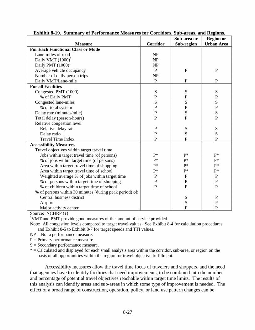
Suggested Measures. Some congestion statistics are useful in areawide analyses, but at

the regional level the questions asked of the transportation analyses often require a broader set of answers. Displaying these statistics will require the analyst to mix a variety of facility-specific and regional summary values. Exhibit 8-19 presents a summary of the information that might be used for corridor, sub-area, and areawide analyses. The level of information would vary depending on the analysis being performed, but the measures are selected to support the types of evaluations and decisions typically made at each level. As noted in the corridor-level discussion, the use of facility- or mode-specific analyses is more appropriate than regional analyses. Accessibility measures become more important as the analysis area is widened or the modal coverage expands.

Average statistics for travel rate and delay rate are useful for intermediate calculations

but most likely will not provide an accurately detailed description of operating conditions within a regional network. Cumulative statistics like Travel Time Index, total delay, congested travel, and congested roadway are more meaningful at this level of analysis. These measures are calculated in the same manner as in the corridor analysis, with sub-totals for measures being calculated for each route (and possibly sub-area) within the regional network.

Exhibit 8-19 shows that individual mode or facility analyses are used to “build up” to the

areawide statistics and can be used in conjunction with areawide analyses. Average vehicle occupancy and daily VMT per lane-mile can be used to evaluate the effect of some types of improvements but are not sufficient for all.

Analyzing all facilities in an area (in the second group of values) requires summary

statistics, but other statistics can also provide information depending on the type of analysis and improvements being studied. Congested travel and facility miles are useful summaries of conditions and can be presented as either (or both) relative to the target measures for areawide studies, or relative to an absolute value such as free-flow travel for national or state “needs” studies.

Accessibility measures are highlighted in Exhibit 8-19 because they focus on the basic

reason for having transportation systems at all: allowing achievement of travel objectives. They measure performance of the transportation system, and its interaction with land use, in how well travel objectives are met.

8-27

Exhibit 8-19. Summary of Performance Measures for Corridors, Sub-areas, and Regions.

Measure Corridor Sub-area or Sub-region

Region or Urban Area

For Each Functional Class or Mode Lane-miles of road NP Daily VMT (1000)1 NP Daily PMT (1000)1 NP Average vehicle occupancy P P P Number of daily person trips NP Daily VMT/Lane-mile P P P For all Facilities Congested PMT (1000) S S S % of Daily PMT P P P Congested lane-miles S S S % of total system P P P Delay rate (minutes/mile) P S S Total delay (person-hours) P P P Relative congestion level Relative delay rate P S S Delay ratio P S S Travel Time Index P P P Accessibility Measures Travel objectives within target travel time Jobs within target travel time (of persons) P* P* P* % of jobs within target time (of persons) P* P* P* Area within target travel time of shopping P* P* P* Area within target travel time of school P* P* P* Weighted average % of jobs within target time P P P % of persons within target time of shopping P P P % of children within target time of school P P P % of persons within 30 minutes (during peak period) of: Central business district S P Airport S P Major activity center P P Source: NCHRP (1) 1VMT and PMT provide good measures of the amount of service provided. Note: All congestion levels compared to target travel values. See Exhibit 8-4 for calculation procedures

and Exhibit 8-5 to Exhibit 8-7 for target speeds and TTI values. NP = Not a performance measure. P = Primary performance measure. S = Secondary performance measure. * = Calculated and displayed for each small analysis area within the corridor, sub-area, or region on the

basis of all opportunities within the region for travel objective fulfillment.

Accessibility measures allow the travel time focus of travelers and shoppers, and the need that agencies have to identify facilities that need improvements, to be combined into the number and percentage of potential travel objectives reachable within target time limits. The results of this analysis can identify areas and sub-areas in which some type of improvement is needed. The effect of a broad range of construction, operation, policy, or land use pattern changes can be

8-28

identified with accessibility measures. Pricing actions that affect demand and travel patterns also change travel time and accessibility.

A few typical measures and geographic scopes are illustrated in Exhibit 8-19, but others

also could be used. The measure of “percent of children within target time of school” was included for a simple illustration of travel market stratification, but the example equally well could have been “percent of commerce (quantified on the basis of employment) within target time of freight distribution centers.”

These analyses can be conducted for either individual improvements or areawide

strategies although they are more effective at the corridor, sub-area, or areawide strategy level. As noted in Exhibit 8-19, accessibility measures are normally calculated for each small area (traffic analysis zone) within the corridor, sub-area, or region being examined, taking into account all of the opportunities for meeting travel objectives within the region as a whole. Maps of the zone by zone results are very instructive in identifying who is most in need and who is most helped by a particular improvement. Zonal level results can be accumulated for the corridor, sub-area, or region as a summary measure, using weighted averages where appropriate.

A limitation is that the magnitude of existing land development and transportation

facilities tends to overwhelm the effect of any new improvements. This causes accessibility measures to represent current features more than the changes accruing from new developments, especially where the new development is focused on achieving a different set of goals. This problem can be addressed by calculating the change in “no-build” alternative. This change will be attributable to the new developments and/or transportation facilities under analysis. This approach will help identify those developments and improvements that contribute to achieving areawide goals for target travel times and accessibility.

Concerns about the effect of “urban sprawl” can be addressed using accessibility

measures. Several different areawide development scenarios can be tested and presented to citizens in a format that can be readily understood. Current and future travel conditions as described by measures such as those in Exhibit 8-18 can be noted, along with such characteristics as percent of trips by mode, the cost of new facilities or operating strategies, and land use patterns. This type of information is much better than the statistics that are currently presented for review in public discussions of long-range planning options. Accessibility measures and associated maps and graphics give transportation land use professionals a method to provide citizens with an idea of the impact of their choices.

The use of accessibility measures will require more computer-based analyses, which

might be perceived as a move away from direct measurement of congestion for some levels of analysis. This does not mean that travel time data will be less useful or less cost-effective to collect. On the contrary, direct measurement of travel time can be used not only to quantify existing conditions but also to calibrate wide-scale models of traffic and transportation system operation and to perform corridor and facility analyses. Geographic information systems are being used to calculate accessibility measures based on planning model travel time and speed output statistics. The typical sequence of events leading up to a public discussion of the alternative improvement plans might be:

8-29

1. Collecting existing traffic condition data directly. 2. Calculating performance measure(s). 3. Comparing results to target conditions that are determined from public comments

during long-range plan discussion. 4. Identifying areas or modes that need improvement. 5. Proposing solutions—areawide strategies will guide which specific improvements are

tested. 6. Testing areawide improvements. 7. Estimating accessibility, mobility, and congestion measures for each strategy or

alternative. 8. Comparing measures to goals. 9. Evaluating and selecting for inclusion in the plan individual mode or facility

improvements that fit with the areawide strategy. 8.2 Discussion of Real-time Data Applications

The examples provided in this chapter thus far have illustrated mobility analysis at

different levels for both arterials and freeways. The data source is assumed to not include incident conditions, and that is why the spreadsheet provides an area for the user to input the percent of incident delay. Therefore, typical data sources for the applications shown thus far might be travel time runs or estimation from demand models.

Direct measurement might also include the use of real-time data sources. This would

include sensors (typically inductance loops) that provide speed, volume, and occupancy data at a given time increment. The Mobility Monitoring Program (2) uses such data to compute congestion performance measures along instrumented freeways of several metropolitan areas in the United States. Certainly data quality and quality control are key issues to consider when processing the real-time data. Computer analysis is required due to the large amount of data that are processed. The MMP annual report discusses these data quality factors in more detail, and it can be reviewed at http://mobility.tamu.edu/mmp. This section of the paper provides insights into how congestion measures can be computed with the real-time data based upon the MMP research. 8.2.1 Congestion and Reliability Measure Calculations

As indicated previously, archived data from the cities participating in MMP consist of traffic speeds and volumes collected at various points along the freeway routes. Because mobility and reliability performance measures are based on travel time, freeway route travel times are estimated from the spot speeds. Exhibit 8-20 illustrates the process whereby lane-by-lane volumes and speeds are used as the basis for estimating freeway route travel times and vehicle-miles of travel. The steps are as follows:

http://mobility.tamu.edu/mmp

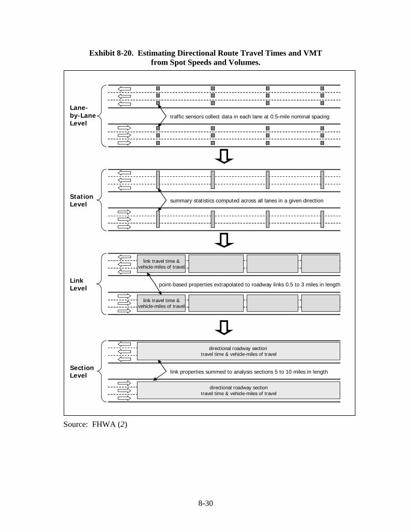
8-30

traffic sensors collect data in each lane at 0.5-mile nominal spacing

summary statistics computed across all lanes in a given direction

link travel time &vehicle-miles of travel

link travel time &vehicle-miles of travel

point-based properties extrapolated to roadway links 0.5 to 3 miles in length

directional roadway sectiontravel time & vehicle-miles of travel

directional roadway section travel time & vehicle-miles of travel

link properties summed to analysis sections 5 to 10 miles in length

Lane-by-LaneLevel

SectionLevel

LinkLevel

StationLevel

Exhibit 8-20. Estimating Directional Route Travel Times and VMT from Spot Speeds and Volumes.

Source: FHWA (2)

8-31

1. If data are reported by lane, the lane-by-lane data are combined into a “station” (e.g., all lanes in a direction). Traffic volumes are summed across all lanes, and traffic speeds are a weighted average, with weighting based on respective traffic volumes.

2. Link properties are estimated from “station” data by assuming that each detector has a

zone of influence equal to half the distance to the detectors immediately upstream and downstream from it. The measured speeds are then assumed to be constant within each zone of influence, and travel times are calculated using the equivalent link lengths. VMT are also computed in this way using traffic volume.

3. Freeway links are then grouped with other similar adjacent links into analysis

sections, which are typically 5 to 10 miles in length. The beginning and end points of analysis sections are typically selected to coincide with major highway interchanges or other locations where traffic conditions are expected to change because of traffic or roadway characteristics.

Travel times for these analysis sections then serve as the basis for all subsequent mobility

and reliability measure calculations. The specifics of these performance measure calculations are contained later in this section. Readers should note that equations using travel time refer to the analysis section travel times as described above.

Several other aspects and definitions used in preparing the archived data for analysis are:

• Holidays are excluded from the weekday peak period analysis, as holidays are

considered to be atypical of normal travel patterns. Holidays are included in several daily total statistics, which also include weekend days. The holidays that are excluded from weekday analyses include: 1. New Year’s Day, 2. Martin Luther King, Jr. Day, 3. President’s Day/Washington’s Birthday, 4. Memorial Day, 5. Independence Day, 6. Labor Day, 7. Thanksgiving Day (and the day after), 8. Christmas (and day before or after, depending on the day of week), and 9. New Year’s Eve.

• Fixed and consistent time periods are defined for all cities. These were:

1. 12:00 a.m. to 6:00 a.m.—early morning, 2. 6:00 a.m. to 9:00 a.m.—morning peak, 3. 9:00 a.m. to 4:00 p.m.—midday, 4. 4:00 p.m. to 7:00 p.m.—afternoon peak, and 5. 7:00 p.m. to 12:00 a.m.—late evening.

• Only mainline freeway detectors are included. Some cities reported ramp data, but

these are dropped to maintain consistency across the cities.

8-32

8.2.2 Computing Congestion Measures with Real-time Data

The Mobility Monitoring Program (2) tracks traffic congestion using the three measures below. For most applications, these measures are reported for the peak periods (6 to 9 a.m. and 4 to 7 p.m.):

• Travel Time Index— (measures congestion intensity, also congestion duration when shown by time of day);

• Percent of congested travel—(measures congestion extent, also congestion duration

when shown by time of day); and

• Total delay—(measures congestion intensity). The Travel Time Index is the ratio of average peak travel time to a free-flow travel time

(Equation 5-2). For MMP, the free-flow conditions are travel times at a speed of 60 mph. Index values can be related to the general public as an indicator of the length of extra travel time spent during a trip. For example, a value of 1.20 means that average peak travel times are 20 percent longer than free-flow travel times. For MMP, the Travel Time Index is calculated for directional freeway sections (as shown in Exhibit 8-20) and then combined into an areawide average by weighting each freeway section by the respective VMT.

The percent of congested travel is calculated as the ratio of congested VMT to total

VMT (Equation 8-1). Note that this is a slightly different form than Equation 5-5 because occupancy for each section is not included. If occupancy values are not different across segments, Equation 5-5 and Equation 8-1 provide the same result. For MMP, a free-flow speed of 60 mph is used as the value below which VMT is considered to be congested.

VMTTotalVMTCongested(%)ravelTdCongesteofPercent = (Eq. 8-1)

Experience indicates that the use of a 60 mph threshold in the percent congested travel

measure may over-represent the magnitude of congestion. In several cities, the spot speeds collected by point-based detectors are less than 60 mph even in light traffic conditions. These point-based detectors are also more likely to record lower speeds than longer distance travel time measurements, due to their common location near entrance ramps and the much greater variation in speed over short sections than long sections. These considerations suggest that a lower speed may be more appropriate for the congestion threshold in this measure when using point-based sensors. Unlike the other congestion measures, congested travel is a binary attribute—travel is either congested or it is not congested, no matter how close the speed is to the congestion threshold. Thus, for a given time period, the VMT is assigned as either congested or not congested, even if the average speeds are just below the congestion threshold. For example, if the nighttime speed limit on an urban freeway system is 55 mph, a significant portion of travel could be categorized as congested without heavy traffic being the cause.

8-33

Delay is calculated as the additional travel time that is incurred when actual travel times are greater than target travel times (Equation 5-1). The delay measure can also be expressed in person-hours in a multimodal context where person travel quantities are known.

8.2.3 Reliability Measures

The congestion measures in the previous section represent the average and total levels of congestion. In addition to average and total statistics, there is a growing recognition of the need to track the variability of congestion and the reliability of travel. The Mobility Monitoring Program tracks these measures for travel reliability:

• Planning Time Index (PPI), and • Buffer Index.

The Planning Time Index is statistically defined as the 95th percentile Travel Time

Index (Equation 8-2) and also represents the extra time most travelers add to a free-flow travel time when planning trips. For example, a Planning Time Index of 1.60 means that travelers should plan for an additional 60 percent travel time above the free-flow travel time to ensure on-time arrival most of the time (95 percent in this report).

( )

( )leminutes/miRate Travel flow-Free

leminutes/miRate Travel Percentile 95

Index Time TravelPercentileIndexTimePlanning

:periodtimeandsectionroadspecificaForth

th== 95 (Eq. 8-2)

The Planning Time Index is useful because it can be directly compared to the Travel

Time Index on similar numeric scales. For example, assume that the peak period Travel Time Index for a particular road section is 1.20, which means that average travel times are 20 percent longer in the peak period than during free-flow conditions. Now assume that the Planning Time Index for that same road and time period is 1.60, which means that 95 percent of all travel times are less than 60 percent longer than during free-flow conditions. In other terms, the Planning Time Index marks the upper limit for the nearly worst (95 percent of the time) travel conditions.

The Buffer Index represents the extra time (buffer) most travelers add to their average

travel time when planning trips (Equation 8-3). The Buffer Index is differentiated from the Planning Time Index in these two important ways:

• The Buffer Index is expressed as a percentage; • The Buffer Index represents the extra time between the average travel time and

near-worst case travel time (95th percentile), whereas the Planning Time Index represents the extra time between the free-flow travel time and the near-worst case travel time (95th percentile).

8-34

(Eq. 8-3)

For example, a Buffer Index of 40 percent means that a traveler should budget an additional 8-minute buffer for a 20-minute average peak travel time to ensure on-time arrival most of the time (95 percent in the examples here). The 95th percentile travel time was chosen for these reliability measures to represent a near-worst case scenario. For example, the 95th percentile travel time corresponds to a 95 percent on-time arrival rate, which can be simply explained in non-technical terms as “being late for work one day per month.” Other percentiles, such as the 85th or 90th percentile, could be used in this or other applications. Ultimately, the application of the reliability measure will determine the percentile used in its calculation.

Equations 8-2 and 8-3 show the reliability measure calculations for a specific road

section and time period. For these reliability measures, the road section and time period should be chosen in a way that accurately represents the reliability of interest. For example, an analysis of urban commuting reliability would likely consider freeway sections 5 to 10 miles in length whose endpoints correspond to major freeway or major arterial interchanges. Alternatively, an analysis of intercity travel reliability would consider much longer freeway sections whose endpoints correspond to popular city origins and destinations. The time period(s) should be selected to include conditions of a similar nature and interest to travelers. For example, a Buffer Index for a typical commuter audience will likely focus on periods throughout the day in which commute travel is made and should not mix travel times from these different periods. That is, travel times from the evening peak period should not be combined into the same distribution as the morning peak travel times when calculating a 95th percentile.

The average planning time or Buffer Index values (across several road sections, time

periods, etc.) can be calculated by using the VMT as a weighting factor (Equation 8-4).

(Eq. 8-4)

8.2.4 Other Considerations for Performance Measure Calculations

The performance measure analysis in MMP uses data in a standard format, which currently consists of 5-minute data (all times of the day and days of the year) for 5- to 10-mile freeway sections. This standard format corresponds with the bottom part of the diagram in

( ) ( ) ( )

( )100%


minutesTime Travel Average -minutes

Time Travel Percentile 95th

% Index Buffer

:period time and sectionroad specifica For

×

=

( )

( )∑

∑

=

=

×= n

iperiodtimeandsectioneachn

n

iperiodtimeandsectioneachnn

VMT

VMTvalueindexValueIndexAverage

:periodstimeandsectionsroadseveralFor

1

1

8-35

Exhibit 8-20. Combining the estimated travel time values or performance measures from each 5-minute time period is accomplished using VMT as a weighting factor for each time period.

Measures that do not use specific origins and destinations generally provide easier

comparisons because these measures are length neutral and can be applied to a wider variety of situations. If trip-based measures are desired as examples for specific origins and destinations, the performance measures described here can be used with the estimated travel time for a specific trip. This combination of generalized, length-neutral measures, as well as specific examples, should provide statistics with which most audiences can relate.

There is no single best performance measure, and users should resist the urge to select a

single measure or index for all situations. Each performance measure reported here addresses different dimensions of traffic congestion or different aspects of reliability. The “dashboard” concept of using a “few good measures” is appropriate (see Chapter 7), and performance monitoring programs should consider selecting a few (for example, two or three of the five presented here) measures for an executive summary or dashboard report.

This analysis defines fixed-length time periods in which to compute average peak period

measures. No single time period will be correct for all analyses, but there are several considerations as follows:

• Peak hour or peak period—Transportation engineers have traditionally used a peak

hour to describe congestion, but major urban areas now experience slow speeds for multiple hours in both the morning and the afternoon. In many areas, congestion growth occurs in the hours before or after the traditional peak hour. Use of a single peak hour misses the congestion that occurs during other times, prompting many areas to define a multi-hour peak period.

• Urban area size—Using a 3- to 4-hour peak period for all area sizes may mask

congestion for the smaller urban areas. Smaller areas can probably develop useful statistics with only peak hour analyses.

• City-to-city comparison—A consistent peak-period length is necessary for any type

of comparison between cities. Comparative studies between urban areas should probably use peak period analyses, rather than only a peak hour.

• Daily or peak comparisons—For national comparisons of reliability trends, a day-

to-day comparison is appropriate. For local purposes, where individual trip planning is also an issue, it may be useful to also include travel reliability within an hour or for several segments of a multi-hour peak period.

8.2.5 Illustration of Mobility Measure Computation Using an ITS Data Source

Exhibit 8-21 shows the results of an investigation of the existing conditions along Southside Freeway assuming the data source is disaggregate ITS data that are aggregated to the peak hour as described in section 8.2 of this white paper. Because the data are from an ITS

8-36

source that inherently includes incident conditions, there is no need for the user to enter a “percent incident delay” as with the other spreadsheet calculations shown in table form in this chapter.

Exhibit 8-21 also shows the computed TTI, BI, and PTI from the ITS data source.

Because of the data source, computation of some of the performance measures is slightly different than prior tables; therefore, a column with a description of how each measure is computed is also included in Exhibit 8-21. One unique difference is that the 95th percentile estimated actual speed is needed to compute the BTI and PTI per Equations 8-2 and 8-3. The average Buffer Index for this section of Southside Freeway is 15 percent and the PTI is 2.00.

8.3 References 1. NCHRP Report 398. Quantifying Congestion—Final Report and User’s Guide. National

Cooperative Highway Research Program Project 7-13, National Research Council, 1997. 2. Monitoring Urban Freeways in 2003: Current Conditions and Trends from Archived

Operations Data. U.S. Department of Transportation, Federal Highway Administration, Report No. FHWA-HOP-05-018, December 2004. Available at: http://mobility.tamu.edu/mmp/.

http://mobility.tamu.edu/mmp/

8-37

Exhibit 8-21. Southside Freeway Existing Operation with ITS Data Source. Roadway Name: Southside Freeway

Location: 71st to 130th Street (Suburban )

Travel Period: Morning Peak Hour

Travel Direction: Northbound (Peak Direction)

Alternative: Existing Operation (ITS Data Source)

Label Measure Units Description

System Element

Total or Average



Auto/Bus Auto/Bus a Length Miles input value 4.4 4.0 8.4 b Vehicle Volume Vehicles collected value 5,800 5,500 c Average Vehicle Occupancy Persons/Vehicle collected value 1.20 1.20 1.20

Speeds

d Free-flow Speed Miles/Hour collected value 65 65 65 e Speed limit Miles/Hour input value 60 60 60 f Target Speed Miles/Hour input value 45 45 45 g Estimated Actual Speed Miles/Hour input value 40 35 38 h 95th Percentile Est. Actual Speed Miles/Hour collected value 34 31 33

Initial Computations i Person Volume Persons b x c 6,960 6,600 13,560 j Vehicle-miles Vehicle-miles a x b 25,520 22,000 47,520 k Person-miles Person-miles i x a 30,624 26,400 57,024

Travel Rates l Free-flow Travel Rate Minutes/Mile 60 / d 0.92 0.92 0.92

m Speed Limit Travel Rate Minutes/Mile 60 / e 1.00 1.00 1.00 n Target Travel Rate Minutes/Mile 60 / f 1.33 1.33 1.33 o Estimated Actual Travel Rate Minutes/Mile 60 / g 1.50 1.71 1.60 p 95th Percentile Est. Actual Speed Minutes/Mile 60 / h 1.76 1.94 1.84

Travel Times t Estimated Actual Travel Time Person-Hours (k x o) / 60 766 754 1,520 Total Delay Rate

v vs. free-flow Minutes/Mile q - m 0.58 0.79 0.68 w vs. speed limit Minutes/Mile q - n 0.50 0.71 0.60 x vs. target Minutes/Mile q - o 0.17 0.38 0.27 y Std. Dev. of Actual Travel Rate Minutes/Mile collected value 0.5 0.5 0.50

Mobility Performance Measures Computations Congested Travel Summary z Person-Miles (vs. target) Person-Miles Sum of congested person-miles

(line k if line v is greater than zero) 30,624 26,400 57,024

ac Person-Hours (vs. target) Person-Hours Sum of congested person hours (line t if line v is greater than zero)

766 754 1,520

af Miles of Congested Roadway (vs. target)

Miles Sum of congested miles (line a if line v is greater than zero)

4.4 4.0 8.40


ai vs. target Percent (ac / t) x 100 100 100 100

Total Delay (vs. target) al Vehicle Travel Vehicle-Hours (j x v) / 60 246 290 536

am Person Travel Person-Hours (k x v) / 60 295 348 643

Total Delay (vs. target) per: ax Person-Mile Person-Minutes (am x 60) / k 0.6 0.8 1.4 ay Mile of Road Person-Hours am / a 67 87 154

Travel Time Index

bd vs. target Travel Rate Ratio o / l 1.63 1.86 1.73

Buffer Index bg Buffer Index Percent ((p - o) / o ) x 100 18 13 15

Planning Time Index

bh vs. free-flow None p / l 1.91 2.10 2.00 Note: See Section 5.4 for further explanation of speed terms and application guidance.

chapter 8—application and interpretation of …

Documents